Multiple Mean-Payoff Optimization under Local Stability Constraints
Abstract
The long-run average payoff per transition (mean payoff) is the main tool for specifying the performance and dependability properties of discrete systems. The problem of constructing a controller (strategy) simultaneously optimizing several mean payoffs has been deeply studied for stochastic and game-theoretic models. One common issue of the constructed controllers is the instability of the mean payoffs, measured by the deviations of the average rewards per transition computed in a finite “window” sliding along a run. Unfortunately, the problem of simultaneously optimizing the mean payoffs under local stability constraints is computationally hard, and the existing works do not provide a practically usable algorithm even for non-stochastic models such as two-player games. In this paper, we design and evaluate the first efficient and scalable solution to this problem applicable to Markov decision processes.
Introduction
Mean payoff, i.e., the long-run average payoff per time unit, is the standard formalism for specifying and evaluating the long-run performance of dynamic systems. The overall performance is typically characterized by a tuple of mean payoffs computed for multiple payoff functions representing expenditures, income, resource consumption, and other relevant aspects. The basic task of multiple mean-payoff optimization is to design a controller (strategy) jointly optimizing these mean payoffs. Efficient strategy synthesis algorithms have been designed for various models, such as Markov decision processes or two-player games (see Related work).
A fundamental problem of the standard mean payoff optimization is the lack of local stability guarantees. For example, consider a payoff function modeling the expenditures of a company. Even if the long-run average expenditures per day (mean payoff) are , there are no guarantees on the maximal average expenditures per day in a bounded time horizon of, say, one month. It is possible that the company pays between and per day every month, which is fine and sustainable. However, it may also happen that there are “good” and “bad” months with average daily expenditures of and , respectively, where the second case is not so frequent but represents a critical cashflow problem that may ruin the company. The mean payoff does not reflect this difference; hence, optimizing the mean payoff (minimizing the overall long-run expenditures) may lead to disastrous outcomes in certain situations.
The lack of local stability guarantees has motivated the study of window mean payoff objectives, where the task is to optimize the average payoff in a “window” of finite length sliding along a run. The window size represents a bounded time horizon (in the above example, the horizon of one month), and the task is to construct a strategy such that the average payoff computed for the states in the window stays within given bounds. Thus, one can express both long-run average performance and stability constraints. For a single payoff function, some technical variants of this problem are solvable efficiently, while others are -hard. For multiple window mean payoffs, intractability results have been established for two-player games (see Related work).
The main concern of the previous works on window mean payoffs is classifying the computational complexity of constructing an optimal strategy. The obtained algorithms are based on reductions to other problems, and their complexity matches the established lower bounds. To the best of our knowledge, there have been no attempts to tackle the high complexity of strategy synthesis by designing scalable algorithms at the cost of some (unavoidable but acceptable) compromises. This open challenge and the problem’s high practical relevance are the primary motivations for our work.
Our Contribution.
We design the first efficient and scalable strategy synthesis algorithm for optimizing multiple window mean payoffs in a given Markov decision process.
We start by establishing the principal limits of our efforts by showing that the problem is -hard even for simple instances where the underlying MDP is a graph. Consequently, every efficient algorithm attempting to solve the problem must inevitably suffer from some limitations. Our algorithm trades efficiency for optimality guarantees, i.e., the computed solutions are not necessarily optimal. Nevertheless, our experiments show that the algorithm can construct high-quality (and sometimes quite sophisticated) strategies for complicated instances of non-trivial size. Thus, we obtain the first practically usable solution to the problem of multiple window mean payoff optimization.
More concretely, the optimization objective is specified by a function Eval measuring the “badness” of the achieved tuple of window mean payoffs, and the task is to minimize the expected value of Eval (we refer to the next section for precise definitions). The Eval function can specify complex requirements on the tuple of achieved mean payoffs. This overcomes another limitation of the previous works, where it was only possible to specify the desired upper/lower bounds for each window mean payoff separately.
The core of our strategy synthesis algorithm is a novel procedure based on dynamic programming, computing the distribution of local mean payoffs for a given starting state. Remarkably, this procedure is differentiable, and the corresponding gradient can be calculated (in the backward pass) at essentially the same computational costs.
A strategy maximizing the expected value of Eval may require memory. Our strategy synthesis algorithm produces finite-memory randomized strategies, where the memory size is a parameter. Using larger memory may produce better strategies but also substantially increases computational costs. From the scalability perspective, using randomization is essential because randomized strategies may achieve much better performance than deterministic strategies with the same amount of memory. This is demonstrated by the simple example below.
Example 1.
Consider a graph with two states and two payoff functions where , , , and . We aim to construct a finite-memory strategy such that the pair of expected window mean payoffs in a window of length is positive in both components and as close to as possible with respect to (Manhattan) distance. Formally, for a given pair of window mean-payoffs , the function Eval returns the distance to the vector if both and are positive; otherwise, Eval returns a “penalty” equal to .
Suppose that the available memory has different states. Then, for every , there is a randomized strategy with memory states achieving a strictly better expected value of Eval than the best deterministic strategy with memory states. For , such strategies are shown in Fig. 1 (for , the best deterministic strategy achieves the window mean payoffs in every window of length , and hence the expected distance to is ; for , of the windows have mean payoffs , and (those beginning with ) have , hence ). The optimal finite-memory strategy achieving the window mean payoffs in every window of length (i.e., the expected value of Eval equal to ) requires memory elements.
In our experiments, we concentrate on the following:
-
(1)
Demonstrating the improvement achieved by the dynamic procedure described above, where the baseline is a “naive” DFS-based procedure.
-
(2)
Evaluating the scalability of our algorithm and the quality of the constructed strategies.
-
(3)
Analyzing the power of randomization to compensate for insufficient memory.
In (2), a natural baseline for evaluating the quality of a constructed strategy is the best value achievable by a finite-memory strategy. However, there is no algorithm for computing the best value. This issue is overcome by constructing a parameterized family of graphs where the best achievable value and the amount of required memory can be determined by a careful manual analysis. The structure of our parameterized graphs is similar to the ones constructed in our -hardness proofs mentioned above. Thus, we avoid bias towards simple instances of the problem. In (3), we analyze the quality of randomized strategies constructed for memory of increasing size. Roughly speaking, our experiments show that even in scenarios where the number of memory elements is insufficient for implementing an optimal strategy, the quality of the obtained strategies is still relatively close to the optimum. Hence, randomization can “compensate” for insufficient memory. This is encouraging because the number of memory elements is one of the crucial parameters influencing the computational costs.
Related Work.
Single mean-payoff optimization for Markov decision processes (MDPs) is a classical problem studied for decades (see, e.g., (Puterman 1994)). For multiple mean-payoff optimization in MDPs, a polynomial-time algorithm computing optimal strategies and approximating the Pareto curve has been given in (Brázdil et al. 2011), and the solution has been successfully integrated into the software tool PRISM (Brázdil et al. 2015).
The window mean payoff objectives have been first studied for a single payoff function and non-stochastic two-player games in (Chatterjee et al. 2015), and then for Markov decision processes in (Bordais, Guha, and Raskin 2019; Brihaye et al. 2020). The complexity of the strategy synthesis algorithms proposed in these works ranges from polynomial time to polynomial space, depending on the concrete technical variant of the problem. The multiple window mean payoff objectives have been considered for two-player games in (Chatterjee et al. 2015), where the problem of computing an optimal strategy is classified as provably intractable (-hard). The optimization objective studied in these works is a simple conjunction of upper/lower bounds imposed on the achieved window mean payoffs. The main focus is on classifying the computational complexity of the studied problems, where the upper bounds are typically obtained by reductions to other game-theoretic problems. To the best of our knowledge, our work gives the first scalable algorithm for multiple window mean payoff optimization applicable to Markov decision processes of considerable size.
In a broader context, a related problem of window parity objective has been studied in (Chatterjee and Henzinger 2006; Horn 2007; Chatterjee, Henzinger, and Horn 2009). An alternative approach to capturing local stability of mean payoff based on bounding the variance of relevant random variables has been proposed in (Brázdil et al. 2017).
The Model
We assume familiarity with basic notions of probability theory (probability distribution, expected value, conditional random variables, etc.) and Markov chain theory. The set of all probability distributions over a finite set is denoted by . We use and do denote the set of non-negative integers and non-negative rationals, respectively.
Markov chains.
A Markov chain is a triple where is a finite set of states, is a stochastic matrix where for all , and is an initial distribution.
A run in is an infinite sequence of states. We use to denote the standard probability measure over the runs of (see, e.g., (Norris 1998))
A state is reachable from a state if for some . We say that is strongly connected (or irreducible) if all states are mutually reachable from each other. For an irreducible , we use to denote the unique invariant distribution satisfying (note that is independent of ). By ergodic theorem (Norris 1998), is the limit frequency of visits to the states of along a run. More precisely, let be a run of . For every , let
where is the number of occurrences of in . If the above limit does not exist, we put . Furthermore, let be the vector of all where . The ergodic theorem says that .
A bottom strongly connected component (BSCC) of is a maximal such that is strongly connected and closed under reachable states. Note that if is irreducible, then the set is the only BSCC of . Otherwise, can have multiple BSCCs, and each such can be seen as an irreducible Markov chain where the set of states is and the probability matrix is the restriction of Prob to .
For the rest of this section, we fix an irreducible Markov chain .
Global and Local Mean Payoff.
Let be a payoff function. For every run , let
be the limit-average payoff per transition along the run . If the limit does not exist, we put . An immediate consequence of the ergodic theorem (see above) is that the defining limit of exists and takes the same value for almost all runs, i.e., . We refer to the (unique) value of as the global mean payoff.
Let be a time horizon. For every , let
be the average payoff computed for the sequence of consecutive states in starting with . We refer to the value as the window mean payoff after steps (assuming some fixed ).
Note that as , the value of is arbitrarily close to with arbitrarily large probability, independently of . However, for a given , the value of depends on and can be rather different from . Also observe that is a discrete random variable, and the underlying distribution depends only on the state . More precisely, for all and such that and , we have that the conditional random variables and are identically distributed. In the following, we write just instead of where .
Mean Payoff Objectives.
Let be payoff functions. The standard multi-objective optimization problem for Markov Decision Processes (see below) is to jointly maximize the global mean payoffs for . In this paper, we use a more general approach where the “badness” of the achieved mean payoffs is measured by a dedicated function . A smaller value of Eval indicates more appropriate payoffs.
For example, the joint maximization of the mean payoffs can be encoded by , where . The defining sum can also be weighted to reflect certain priorities among the Pareto optimal solutions. In general, Eval can encode the preference of keeping the mean payoffs close to some values, within some interval, or even enforce some mutual dependencies among the mean payoffs.
As we shall see, our strategy synthesis algorithm works for an arbitrary Eval that is decomposable. Intuitively, the decomposability condition enables more efficient evaluation/differentiation of Eval by dynamic programming without substantially restricting the expressive power.
Now we can define the global and local value of a run as follows:
where and are the global and window mean payoff determined by . Note that corresponds to the “limit-average badness” of the window mean-payoffs along the run .
Clearly, , where . Furthermore, by applying the ergodic theorem and the above observations leading to the definition of , we obtain that where
| (1) |
We refer to gval and wval as the global and window mean payoff value. In this paper, we study the problem of minimizing wval in a given Markov decision process.
Markov decision processes.
A Markov decision process (MDP)111Our definition of MDPs is standard in the area of graph games. Although it is equivalent to the “classical” MDP definition of (Puterman 1994), it is more convenient for our purposes and leads to simpler notation. is a triple where is a finite set of vertices partitioned into subsets of non-deterministic and stochastic vertices, is a set of edges s.t. each vertex has at least one out-going edge, and is a probability assignment such that only if . We say that is a graph if .
Outgoing edges in non-deterministic vertices are selected by a strategy. In this paper, we consider finite-memory randomized (FR) strategies where the selection depends not only on the vertex currently visited but also on some finite information about the history of vertices visited previously.
FR strategies.
Let be an MDP and a finite set of memory states that are used to “remember” some information about the history. For a given pair where is a currently visited vertex and a current memory state, a strategy randomly selects a new pair such that .
Formally, let be a memory allocation, and let be the set of augmented vertices. A finite-memory (FR) strategy is a function such that for all where and every we have that
An FR strategy is memoryless (or Markovian) if is a singleton. In the following, we use to denote an augmented vertex of the form for some .
Every FR strategy together with a probability distribution determine the Markov chain where .
The Optimization Problem
In this section, we define the multiple window mean-payoff optimization problem and examine the principal limits of its computational tractability.
Let be an MDP, payoff functions, and an evaluation function. Furthermore, let be a time horizon. The task is to construct an FR strategy and an initial augmented vertex so that the value of wval is minimized.
More precisely, for a given FR strategy , the function wval is evaluated as follows. Every is extended to the augmented vertices of by defining . Let be the BSCCs of the Markov chain . Recall that every can be seen as an irreducible Markov chain. We use to denote the window mean payoff value computed for . The value of wval achieved by , denoted by , is defined as
Recall that the initial augmented vertex can be chosen freely, which is reflected in the above definition (the strategy can be initiated directly in the “best” BSCC and thus achieve the value ).
A FR-strategy is -optimal for a given if
where ranges over all FR strategies. A -optimal strategy is called optimal.
The next theorem shows that computing an optimal strategy is computationally hard, even for restricted subsets of instances.
Theorem 1
Let be a graph, payoff functions, a time horizon, and Eval an evaluation function. The problem of whether there exists a FR strategy such that is -hard.
Furthermore, the problem is -hard even if the set of eligible instances is restricted so that an optimal memoryless strategy is guaranteed to exist, and one of the following three conditions is satisfied:
-
A.
(i.e., there is only one payoff function).
-
B.
, and there are thresholds such that iff and .
-
C.
There is a constant such that (i.e., the number of payoff functions is “substantially smaller” than the number of vertices), and the co-domain of every is .
Intuitively, (A) says that one payoff function is sufficient for -hardness, (B) says that for two payoff functions we have -hardness even if we just aim to push both window mean payoffs above certain thresholds, and (C) says that the range of all payoff functions can be restricted to even if the number of payoff functions is at most . Furthermore, the Eval function can be constructed so that it ranges over where is an arbitrary constant, and iff is optimal. Consequently, an optimal (and even -optimal) strategy cannot be constructed in polynomial time unless .
The Algorithm
For the rest of this section, we fix an MDP , a time horizon , payoff functions , and an evaluation function Eval.
Our algorithm is based on optimizing wval by the methods of differentiable programming. The core ingredient is a dynamic procedure for computing the expected value of (see (1)). The procedure is designed so that the gradient of wval can be computed using automatic differentiation. Then, we show how to incorporate this procedure into a strategy-improvement algorithm for wval. For the rest of this section, we fix a memory allocation .
Representing FR Strategies.
For every pair of augmented vertices such that , we fix a real-valued parameter representing . Note that if is stochastic, then the parameter actually represents the probability of selecting the memory state of . These parameters are initialized to random values, and we use the standard Softmax function to transform these parameters into probability distributions. Thus, every function depending on becomes a function of the parameters, and we use to denote the corresponding gradient.
Computing .
Let be an FR strategy where is the memory allocation. We show how to compute interpreted as a function of the parameters representing .
Recall that . Hence, the first step is to compute all BSCCs of by the Tarjan’s algorithm (Tarjan 1972). Then, for each BSCC , we compute in the following way.
The invariant distribution is computed as the unique solution of the following system of linear equations: For every , we fix a fresh variable and the corresponding equation . Furthermore, we add the equation . Recall that is the unique distribution satisfying , where is the probability matrix of . Hence, is the unique solution of the constructed system.
Computing the Expected Value of Eval by Dynamic Programming.
In this section, we show how to compute (2) by dynamic programming for a given . We use to denote the probability measure over the runs in , where the initial distribution assigns to .
Let be the set of vectors of non-negative integers indexed by the augmented vertices . For each , let , where . For every , let be an indicator assigning to every run of either or so that iff for every .
Calculating (3) directly is time-consuming. However, is the same for many different , and our dynamic algorithm avoids these redundant computations. The algorithm is applicable to a subclass of decomposable Eval functions defined below. The decomposability condition is not too restrictive, and it does not influence the -hardness of the considered optimization problem (the Eval functions constructed in the proof of Theorem 1 are decomposable).
For all and , we write if and for all . We say that Eval is decomposable if there is a set of representatives and efficiently computable functions , and satisfying the following conditions:
-
•
for every , i.e., the value of Eval for a given is efficiently computable by the function just from the representative of .
-
•
For each , we have that . That is, when a path is prolonged by a vertex , the representative can be efficiently updated by the function .
A concrete example of a decomposable Eval and the associated functions is given in a special subsection below.
For each , let . Furthermore, for every representative , let . Then (3) can be rewritten into
| (4) |
Algorithm 1 computes for all and by dynamic programming. Moreover, only reachable representatives (i.e., those with ) are considered during the computation. Thus, Algorithm 1 avoids the redundancies of the direct computation of (3).
More specifically, Algorithm 1 uses two associative arrays (such as C++ unordered_map), called and , to gather information about the representatives and the corresponding probabilities. In the -th iteration of the cycle, contains items corresponding to all reachable , and the items corresponding to all reachable are gradually gathered in . In particular, each is indexed by the elements . Intuitively, each such element represents the set of all runs initiated in such that there exists satisfying , , and . The value associated to is the total probability of all such runs .
A Simple DFS Procedure.
As a baseline for measuring the improvement achieved by the dynamic algorithm described in the previous paragraph, we use a simple DFS-based procedure of Algorithm 2. For simplicity, the vector is denoted by .
The DFS procedure inputs the following parameters:
-
•
the current augmented vertex ;
-
•
the probability of the current path;
-
•
the length of the current path;
-
•
the vector of the individual payoffs accumulated along the path.
The procedure is called as DFS() for each in the currently examined BSCC . At the end of the computation, the global variable holds the value of (2).
A Strategy Improvement Algorithm.
In this section, we describe a strategy improvement algorithm WinMPsynt that inputs an MDP , payoff functions , a decomposable , and a time horizon , and computes an FR strategy with the aim of minimizing .
The memory allocation function is a hyperparameter (by default, all memory states are assigned to every vertex). The algorithm proceeds by randomly choosing the parameters representing a strategy. The values are sampled from LogUniform distribution so that no prior knowledge about the solution is imposed. Then, the algorithm computes the BSCCs of and identifies a BSCC with the best . Subsequently, is improved by gradient descent. The crucial ingredient of WinMPsynt is Algorithm 1, allowing to compute and its gradient by automatic differentiation. After that, the point representing the current strategy is updated in the direction of the steepest descent. The intermediate solutions and the corresponding values are stored, and the best solution found within Steps optimization steps is returned (the value of Steps is a hyper-parameter). Our implementation uses PyTorch framework (Paszke et al. 2019) and its automatic differentiation with ADAM optimizer (Kingma and Ba 2015). Observe that WinMPsynt is equally efficient for general MDPs and graphs. The only difference is that stochastic vertices generate fewer parameters.
An Example of a Decomposable Eval Function.
Let Pay be a payoff function, and let where is either or depending on whether or not, respectively. Assume . Then, we can put and define
Note that as soon as the accumulated payoff exceeds , there is no reason to remember the exact value because Eval inevitably becomes one. Note that contains elements independently of the size of , while the total number of all such that may exceed , and the total number of paths, all of which are considered separately by the naive DFS-based algorithm, may reach .
Experiments
We perform our experiments on graphs to separate the probabilistic choice introduced by the constructed strategies from the internal probabilistic choice performed in stochastic vertices. The graphs are structurally similar to the ones constructed in the -hardness proof of Theorem 1. This avoids bias towards simple instances. Recall that the problem of constructing a (sub)optimal strategy for such graphs is -hard even if just one memory state is allocated to every vertex, there are only two payoff functions, and we aim at pushing the window mean payoffs above certain thresholds (see item B. in Theorem 1).
The graphs .
For every , we construct a directed ring with three “layers” where every vertex in the inner, middle, and outer layer is assigned a pair of payoffs , , and , respectively. The vertices are connected in the way shown in Fig. 2.
The Eval function.
A scenario is a pair where are even integers in the interval representing and the window length . For every scenario, we aim to push both window mean payoffs simultaneously above a bound , where is as large as possible. For each , the maximal bound achievable by an FR strategy is denoted by , and can be determined by a careful manual analysis, together with the least number of memory states required by an optimal FR strategy (we have that for all ). Let us note that the manual analysis of is enabled by the regular structure of , but this regularity does not bring any advantage to WinMPsynt.
For a given scenario , we use the evaluation function defined as follows:
By the definition of , there always exists an optimal FR strategy for the scenario achieving the bound , i.e., . Due to the normalizing denominator, the maximal value of is bounded by , simplifying the comparison of strategies constructed for different scenarios.
The experiments.
For all scenarios and , we invoked WinMPsynt times, where the underlying memory allocation assigns memory elements to every vertex, and the number of optimization steps is set to . Thus, for every and every , we obtained a set of strategies and the corresponding values. We also use to denote , and to denote the union of all .
The quality of the obtained strategies.
Due to the definition of , for every , the value can be interpreted as a normalized distance to the optimal strategy with value . The percentage of scenarios where the value of the best strategy found by WinMPsynt is bounded by , , and is , , and , respectively. Hence, the best strategies found by WinMPsynt are of very high quality. Since the best strategy is selected out of strategies constructed for a given scenario, a natural question is how good are these strategies “on average”. The percentage of all whose value is bounded by , , and is , , and , respectively. Hence, the quality of an “average” strategy is substantially worse, which is consistent with intuitive expectations (since the problem is computationally hard, obtaining a high-quality solution for non-trivial instances cannot be easy).
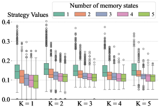
The roles of memory states and randomization are demonstrated in Fig. 3. The scenarios are split into five disjoint subsets with the same (horizontal axis). For each subset, we report the values achieved by strategies with memory states assigned to every vertex (indicated by different colors). Note that for the subset where , an optimal strategy is computed when or more memory states are available. For the subset where , an optimal strategy is found only for memory states. For all subsets, increasing the number of memory states decreases the average strategy value. Furthermore, even if the number of memory states is smaller than , the value of the constructed strategies is still relatively small on average. Hence, randomization effectively compensates for the lack of memory.
The improvement achieved by dynamic programming.
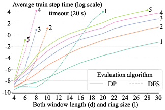
The baseline for evaluating the efficiency improvement achieved by the dynamic procedure of Algorithm 1 is the simple DFS-based procedure of Algorithm 2. For every instance where , we report the average running time of one training step for an FR strategy with memory states (different colors) using logarithmic scale. The timeout is set to secs. For one memory state, the DFS-based procedure reaches the timeout for all scenarios where , whereas the dynamic procedure needs less than one second even for the scenario. Hence, the dynamic procedure substantially outperforms the DFS-based one, and the same holds when the number of memory states increases.
Conclusions
We have designed an efficient strategy synthesis algorithm for optimizing multiple window mean payoffs capable of producing high-quality solutions for instances of considerable size. An interesting question is whether the proposed approach is applicable to a larger class of window-based optimization objectives such as the window parity objectives.
References
- Bordais, Guha, and Raskin (2019) Bordais, B.; Guha, S.; and Raskin, J.-F. 2019. Expected Window Mean-Payoff. In Proceedings of FST&TCS 2019, volume 150 of Leibniz International Proceedings in Informatics, 32:1–32:15. Schloss Dagstuhl–Leibniz-Zentrum für Informatik.
- Brázdil et al. (2011) Brázdil, T.; Brožek, V.; Chatterjee, K.; Forejt, V.; and Kučera, A. 2011. Two Views on Multiple Mean-Payoff Objectives in Markov Decision Processes. In Proceedings of LICS 2011. IEEE Computer Society Press.
- Brázdil et al. (2015) Brázdil, T.; Chatterjee, K.; Forejt, V.; and Kučera, A. 2015. MultiGain: A Controller Synthesis Tool for MDPs with Multiple Mean-Payoff Objectives. In Proceedings of TACAS 2015, volume 9035 of Lecture Notes in Computer Science, 181–187. Springer.
- Brázdil et al. (2017) Brázdil, T.; Chatterjee, K.; Forejt, V.; and Kučera, A. 2017. Trading performance for stability in Markov decision processes. Journal of Computer and System Sciences, 84: 144–170.
- Brihaye et al. (2020) Brihaye, T.; Delgrange, F.; Oualhadj, Y.; and Randour, M. 2020. Life is Random, Time is Not: Markov Decision Processes with Window Objectives. Logical Methods in Computer Science, 16(4).
- Chatterjee et al. (2015) Chatterjee, K.; Doyen, L.; Randour, M.; and Raskin, J.-F. 2015. Looking at Mean-Payoff and Total-Payoff through Windows. Information and Computation, 242: 25–52.
- Chatterjee and Henzinger (2006) Chatterjee, K.; and Henzinger, T. 2006. Finitary winning in -regular games. In Proceedings of TACAS 2006, volume 3920 of Lecture Notes in Computer Science, 257–271. Springer.
- Chatterjee, Henzinger, and Horn (2009) Chatterjee, K.; Henzinger, T.; and Horn, F. 2009. Stochastic games with finitary objectives. In Proceedings of MFCS 2009, volume 5734 of Lecture Notes in Computer Science, 34–54. Springer.
- Horn (2007) Horn, F. 2007. Faster Algorithms for Finitary Games. In Proceedings of TACAS 2007, volume 4424 of Lecture Notes in Computer Science, 472–484. Springer.
- Kingma and Ba (2015) Kingma, D. P.; and Ba, J. 2015. Adam: A Method for Stochastic Optimization. In Proceedings of ICLR 2015.
- Norris (1998) Norris, J. 1998. Markov Chains. Cambridge University Press.
- Paszke et al. (2019) Paszke, A.; Gross, S.; Massa, F.; Lerer, A.; Bradbury, J.; Chanan, G.; Killeen, T.; Lin, Z.; Gimelshein, N.; Antiga, L.; Desmaison, A.; Kopf, A.; Yang, E.; DeVito, Z.; Raison, M.; Tejani, A.; Chilamkurthy, S.; Steiner, B.; Fang, L.; Bai, J.; and Chintala, S. 2019. PyTorch: An Imperative Style, High-Performance Deep Learning Library. In Advances in Neural Information Processing Systems 32, 8024–8035. Curran Associates, Inc.
- Puterman (1994) Puterman, M. 1994. Markov Decision Processes. Wiley.
- Tarjan (1972) Tarjan, R. 1972. Depth-First Search and Linear Graph Algorithms. SIAM Journal of Computing, 1(2).
Supplementary Material
Appendix A A Proof of Theorem 1
Let us start by restating the theorem.
Theorem 2
Let be a graph, payoff functions, a time horizon, and Eval an evaluation function. The problem of whether there exists a FR strategy such that is -hard.
Furthermore, the problem is -hard even if the set of eligible instances is restricted so that an optimal memoryless strategy is guaranteed to exist, and one of the following three conditions is satisfied:
-
A.
(i.e., there is only one payoff function).
-
B.
, and there are thresholds such that iff and .
-
C.
There is a constant such that (i.e., the number of payoff functions is “substantially smaller” than the number of vertices), and the co-domain of every is .
For every , let be the graph where
-
•
;
-
•
contains the edges , , , for every , where .
-
•
since is a graph, the probability assignment is empty.
The structure of is shown in Fig. 5. The cases A.–C. are considered separately.
Case A.
An instance of the Subset Sum problem is a sequence of positive integers and another positive integer . The question is whether this sequence contains a subsequence such that the sum of all elements in the subsequence is equal to . The Subset Sum is one of the standard -complete problems (all are written in binary)
For a given instance , of Subset Sum, consider the graph and the payoff function Pay such that
-
•
, and for all ,
-
•
and for all .
Observe that contains a subsequence with a sum of iff there is a path of the form where every is either or such that the total payoff accumulated along this path is equal to .
We show that the latter condition is equivalent to the existence of a FR strategy such that , where and is the absolute value of . This proves the -hardness of Case A.
Clearly, if there is a path such that every is either or and the total payoff accumulated along this path is equal to , then there exists a memoryless strategy for such that ( simply follows the path forever, using the edge ).
Now let be an FR strategy such that . Then, because Eval is non-negative. Let be a BSCC of such that . Due to the structure of , there is an augmented vertex of the form . Then, together with the next augmented vertices visited with some positive probability inevitably form a path of the form where every is either or . Observe that the total payoff accumulated along this path must be zero (if it was positive or negative, then , and we have a contradiction). Since the underlying path has the same accumulated payoff equal to , we are done.
Case B.
Here we use a reduction from the -complete Knapsack problem. An instance of Knapsack is a finite sequence , where all and are positive integers, together with two positive integer bounds . The question is whether there exists a subsequence such that the sum of all ’s is at least , and the sum of all ’s is at most . We assume that (otherwise the instance could be solved trivially by checking whether ).
For a given instance , , of Knapsack, let , and consider the graph and two payoff functions such that
-
•
, for all ,
-
•
, for all ,
-
•
, for all .
Let , , , and
Clearly, , and , hence .
Similarly as in Case A., one can easily verify that
-
•
if , , is a positive instance of Knapsack, then there exists a memoryless startegy such that .
-
•
if there exists a FR strategy such that , then , , is a positive instance of Knapsack.
Case C.
The Sat problem is the question of whether a given propositional formula is satisfiable. The Sat problem is -complete even for formulae of the form where each is a disjunction of literals over (a literal is a propositional variable or its negation). Furthermore, the problem remains -complete if we additionally assume that , where is an arbitrary constant.
For a given formula over the propositional variables , consider the graph and the payoff functions such that, for every , the following holds:
-
•
for all ;
-
•
for all , we have that equals or , depending on whether occurs in the clause or not, respectively;
-
•
for all , we have that equals or , depending on whether occurs in the clause or not, respectively.
Observe that the co-domain of is , and because .
Let be either or depending on whether each is positive or not, respectively. Furthermore, let . Now it is easy to check the following:
-
•
If is satisfiable, then there exists a path in of the form such that the vector of accumulated total payoffs is positive in every component. Hence, there is a memoryless strategy such that .
-
•
If there is FR strategy such that , then there is a path in of the form such that the vector of accumulated total payoffs is positive in every component (here we argue similarly as in Case A.) Note that this path determines a satisfying assignment for the formula, where is true iff the vertex occurs in the path.
Note that in all of the considered cases, the Eval function can be trivially adjusted so that it returns either or a given constant , depending on whether the given payoff (or tuple of payoffs) corresponds to a satisfying subsequence/assignment or not, respectively. This implies that the problem of constructing a -optimal strategy is also computationally hard.
Appendix B Experiments
In this section, we give more details about the experiments. The quality of the best strategies constructed by WinMPsynt for each scenario is reported in Table 1. More precisely, the table shows the percentage of scenarios where the value of the best strategy found by WinMPsynt is below a given threshold.
| Bound on | of scenarios |
|---|---|
| 0.0 | 40 % |
| 0.01 | 42 % |
| 0.02 | 42 % |
| 0.03 | 43 % |
| 0.04 | 49 % |
| 0.05 | 52 % |
| 0.06 | 66 % |
| 0.07 | 78 % |
| 0.08 | 90 % |
| 0.09 | 98 % |
| 0.1 | 100 % |
Similar statistics for the set of all of the strategies constructed by WinMPsynt for all scenarios are given in Table 2.
As we already noted, the best strategies constructed by WinMPsynt are of very high quality. The value of an “average” strategy is not so close to the optimum due to the high computational complexity of the considered optimization problem.
| Bound on the value | of strategies |
|---|---|
| 0.0 | 6 % |
| 0.1 | 27 % |
| 0.2 | 95 % |
| 0.3 | 99.8 % |
| 0.4 | 99.9 % |
| 0.5 | 100 % |
Theorem 3
Let be even positive integers. Then .
We will first show that . Let , since is even and positive, then is a non-negative integer. Consider a FR strategy that starts in the middle layer. It then moves along the inner layer times, moves back into the middle layer, and moves times in the outer layer, finally it returns back to the middle layer. This pattern has a total length equal to . If we repeat this pattern times, we get a cycle of length which can be easily represented as an FR strategy.
Moreover, in each window of length we have exactly on both payoffs. Hence we can satisfy a bound .
The other inequality is easy to see, as one would need to sacrifice going in the inner layer for going more in the outer or vice versa.
Values of
The analysis for was done by an algorithm that computes the memory needed for the optimal strategy described above.
The values for when both and are even positive integers are reported in Table 3.
| d = | 2 | 4 | 6 | 8 | 10 | 12 | 14 | 16 | 18 | 20 |
|---|---|---|---|---|---|---|---|---|---|---|
| r=20 | 1 | 1 | 1 | 2 | 1 | 2 | 3 | 2 | 4 | 1 |
| r=18 | 1 | 2 | 1 | 2 | 2 | 2 | 3 | 4 | 1 | 5 |
| r=16 | 1 | 1 | 1 | 1 | 2 | 2 | 3 | 1 | 4 | 3 |
| r=14 | 1 | 2 | 1 | 2 | 2 | 3 | 1 | 4 | 4 | 5 |
| r=12 | 1 | 1 | 1 | 2 | 2 | 1 | 3 | 2 | 2 | 3 |
| r=10 | 1 | 2 | 1 | 2 | 1 | 3 | 3 | 4 | 4 | 2 |
| r=8 | 1 | 1 | 1 | 1 | 2 | 2 | 3 | 2 | 4 | 3 |
| r=6 | 1 | 2 | 1 | 2 | 2 | 2 | 3 | 4 | 2 | 5 |
| r=4 | 1 | 1 | 1 | 2 | 2 | 2 | 3 | 2 | 4 | 3 |
| r=2 | 1 | 2 | 1 | 2 | 2 | 3 | 3 | 4 | 4 | 5 |