Alternative Channel Charting Techniques in Cellular Wireless Communications

Abstract

We investigate the use of conventional angle of arrival (AoA) algorithms the Bartlett’s algorithm, the Minimum Variance Distortion Response (MVDR or Capon) algorithm, and the Minimum Norm algorithm for estimating the AoA $\theta$ together with our previously introduced algorithms linear regression (LR), inverse of the root sum squares of channel coefficients (ISQ), as well as a novel use of the MUSIC algorithm for estimating the distance from the base station, $\rho$ in the context of channel charting. We carry out evaluations in terms of the visual quality of the channel charts, the dimensionality reduction performance measures trustworthiness (TW) and connectivity (CT), as well as the execution time of the algorithms. We find that although the Bartlett’s algorithm, MVDR, and Minimum Norm algorithms have sufficiently close performance to techniques we studied earlier, the Minimum Norm algorithm has significantly higher computational complexity than the other two. Previously, we found that the use of the MUSIC algorithm for estimation of both $\theta$ and $\rho$ has a very high performance. In this paper, we investigated and quantified the performance of the Bartlett algorithm in its use for estimating both $\theta$ and $\rho$, similar to the our previously introduced technique of using MUSIC for estimating both.

I Introduction

A channel chart is a chart created from channel state information (CSI). It has the property of preserving the relative geometry of the radio environment consisting of a base station (BS) and user equipments (UEs) [1]. By employing this chart, the BS locates the relative locations of the UEs. This has the potential of enabling many applications such as handover, cell search, user localization, etc. While most of the works on this subject employed estimation of a channel chart using dimensionality reduction techniques, in this paper we calculate the channel chart directly by using model-based approaches.

Figure 1: Summary of channel charting via dimensionality reduction [1].

We will begin our discussion by Fig. 1, which is a redrawn and simplified version of [1, Fig. 3]. UE transmitters are located in spatial geometry $\mathbb{R}^{D}$, where $D=2$ or $3$ [1]. The BS receiver calculates CSI in radio geometry $\mathbb{C}^{M}$ where $M\gg D$. Then, a channel chart is created in $\mathbb{R}^{D^{\prime}}$ where $D^{\prime}\leq D$ such that the representation in $\mathbb{R}^{D^{\prime}}$ preserves the local geometry of the original spatial locations in $\mathbb{R}^{D}$, in other words, the relative positions of the UEs. Reference [1] introduces and compares three dimensionality reduction algorithms, namely principal component analysis (PCA), Sammon’s mapping (SM), and autoencoder (AE). PCA is a linear technique for dimensionality reduction. It maps a high-dimensional point set (e.g., CSI features) into a low-dimensional point set (e.g., the channel chart) in an unsupervised approach. It does so by performing dimensionality reduction only for the data points used in calculations. It does not form a function one can use to perform dimensionality reduction for future data points. For that reason, strictly speaking, it is not a machine learning (ML) algorithm, although sometimes it is quoted as an unsupervised ML algorithm. SM is a nonlinear method for dimensionality reduction which retains small pairwise distances between the two point sets [1]. Similarly to PCA, it does not form a function for dimensionality reduction of future data points. Whereas, an AE is a deep artificial neural network used for unsupervised dimensionality reduction [1]. Unlike PCA and SM, it does perform learning. Thus, it can be used for future data points.

Consider Fig. 1. In this figure, there are four blocks to carry out channel charting. In the upper left, the spatial geometry in $\mathbb{R}^{D}$ is depicted. In the upper right block, the radio geometry in $\mathbb{C}^{M}$ is calcaulated. The lower blocks perform feature extraction and forward charting to create channel charts. In the approach in this paper we keep the upper two blocks, as in [2, 3, 4]. In our approach, one replaces the lower two blocks with model-based techniques to directly determine the angle of arrival and the distance from the BS of the UE. Thus, the relative positions of the UEs with respect to the BS are preserved, and the basic goal of channel charting is automatically satisfied.

II Channel Models

We employ three channel models, namely vanilla line-of-sight (LOS), Quadriga LOS (QLOS), and Quadriga non-LOS (QNLOS) [5, 6, 7]. These are the same models used in [1], as well as our papers [2, 3, 4]. We start with the simplest, vanilla LOS. Vanilla LOS is one LOS ray described as

$$h=\rho^{-r}\;e^{-j\left(\frac{2\pi\rho}{\lambda}+\phi\right)}$$ (1)

where $\rho$ is the distance between the transmitter and the receiver and $r$ is known as the path loss exponent. In (1), the first term in the channel phase is linearly proportional with the distance $\rho$. The second term $\phi$ is a uniformly distributed random variable in $[0,2\pi)$. The channel amplitude is a random variable (Rician (QLOS) or Rayleigh (QNLOS)) which is inversely proportional to the distance square for free space, ${\sim}\rho^{-2}$, i.e., the path loss exponent $r=2$.

TABLE I: Simulation parameters.

Parameter	Value
Antenna array	Uniform Linear Array (ULA)
	with spacing $\lambda/2=7.495$ cm
Number of array antennas	32
Number of transmitters (UEs)	2048
Carrier frequency	2.0 GHz
Bandwidth	312.5 kHz
Number of clusters	0
Number of subcarriers	1 (up to 32 in the case of the
	MM algorithm (Sec. III-B3))

Next we discuss the Quadriga channel model [5, 6, 7]. Quadriga stands for quasi deterministic radio channel generator. It is a statistical three-dimensional geometry-based stochastic channel model employing ray tracing. According to [5], it has the following features: i) three-dimensional propagation (antenna modeling, geometric polarization, scattering clusters), ii) continuous-time evolution, iii) spatially correlated large- and small-scale fading, and iv) transition between varying propagation scenarios. The Quadriga model is very customizable. It has many features and details. The model was validated by measurements in downtown Dresden, Germany [7, Ch. 4] and in downtown Berlin, Germany [7, Ch. 5]. In this paper we used the parameters in Table I with the Urban Macro-Cell (UMa) version of the Quadriga mode in the simulations. Some details of the measurement setup are available in [5, Sec. III], in specific detail in [5, Table II].

The signal-to-noise ratio (SNR) in channel model is calculated by considering the power in the received signal ($P_{r}$) and the power in the noise measured at the receiver ($P_{n}$). We note that while the estimated channel would have some noise added to it, the most significant component of the noise at the receiver is additive white Gaussian thermal noise. Then, the SNR at the receiver is given as $\textrm{SNR}=P_{r}/P_{n}$ where $P_{r}$ takes into account the transmitted power and the channel model, see, e.g., Sec. II-B in [8]. In the code [9] which we used as the basis for our simulations, the calculation of SNR is carried out by normalizing $P_{r}$ and then properly scaling the additive white Gaussian thermal noise power $P_{n}$ for all three channel models.

III Estimating the Coordinates ${\theta}$ and ${\rho}$

We will use the symbol $\theta$ for the angle of arrival (AOA) and $\rho$ for the distance between the BS and the UE. Note that one can estimate $\theta$ and $\rho$ concurrently because they do not depend on each other. In this section, we will first discuss how to estimate $\theta$ by using the MUSIC algorithm and then we will discuss three algorithms to estimate $\rho$.

III-A Estimating $\theta$ Using MUSIC

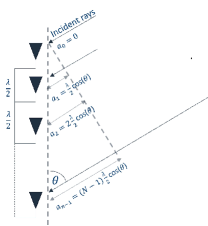
Figure 2: Angle of arrival $(\theta)$ relation with phase.

Consider Fig. 2. One can see from this figure that each antenna element receives a ray which travels an additional distance $\frac{\lambda}{2}\cos(\theta)$ as compared to the previous element. As a result, the incremental phase shift for each antenna element is $e^{j\pi\cos(\theta)}$. Thus, one can compose the steering vector

$${\bf A}(\theta)=(1,e^{j\pi\cos(\theta)},e^{j\pi 2\cos(\theta)},\ldots,e^{j\pi(N_{R}-1)\cos(\theta)})^{T},$$ (2)

where $N_{R}$ is the number of receive antennas at the BS. This vector is employed in determining the AOA as well as in beamforming applications.

Algorithm 1 MUSIC Procedure for Estimating $\theta$

Calculate the CSI across antennas and subcarriers covariance matrix ${\bf R}$ = $\mathbb{E}[{\bf h}{\bf h}^{H}]$

Get the eigenvectors and eigenvalues of R

Separate system subspace $\cal S$ and noise subspace $\cal N$ by defining a threshold

Calculate ${\bf N}$ by concatenating the eigenvectors of $\cal N$

for $\theta=0:180$ in increments of 1 do

  Calculate the steering vector ${\bf A}(\theta)$

  Calculate the $\textrm{PMF}(\theta)=\frac{1}{\textrm{Norm}_{2}({\bf N}^{H}{\bf A}(\theta))}$

end for

Search the PMF for a peak and find the corresponding $\theta$

The steering vector ${\bf A}(\theta)$ is embedded within the CSI correlation matrix (${\bf R}=\mathbb{E}[{\bf h}{\bf h}^{H}]$), where ${\bf h}$ is the received channel vector at the BS along with noise. The vector ${\bf h}$ is $N_{R}\times 1$ where $N_{R}$ is the number of antennas at the BS. By decomposing $\bf R$ into its eigenvectors and examining the corresponding eigenvalues, the eigenvectors can be separated into a signal subspace $\cal S$ and a noise subspace $\cal N$. This is achieved by using the fact that the noise eigenvectors will correspond to very small eigenvalues compared to the signal space eigenvalues. The two subspaces $\cal S$ and $\cal N$ are orthogonal. Let’s assume that the dimensionality of the noise subspace $\cal N$ is $p$. Form the matrix ${\bf N}$ (dimension $N_{R}\times p$) by concatenating the eigenvectors of $\cal N$. The multiplication of the noise subspace eigenvectors matrix $\bf N$ and the steering vector will be almost zero. We can use this concept to find the correct angle by sweeping $\theta$ in the steering vector as described in Algorithm 1 where PMF($\theta$) is a probability mass function within a scale of constant.

III-B Estimating $\rho$

We will now discuss three methods on how to estimate $\rho$ [2]. Please refer to (1) with $r=2$. This is the simple channel ray model we will employ below.

III-B1 Estimating $\rho$ Using ISQ

In this method, we calculate the square root inverse of the sum of CSI magnitudes for all antennas as

$$\rho=\frac{1}{\sqrt{\sum_{n=0}^{N_{R}-1}{\rm abs}(h_{n})}},$$ (3)

where $h_{n}$ is the channel between the UE and the $n$-th antenna at the BS and $N_{R}$ is the number of antennas at the base station. We call this algorithm as ISQ (inverse square root sum). The algorithm is motivated by (1) with the path loss component $r=2$. In (3), $\rho={1}/\sqrt{{\rm abs}(h_{n})}$ is calculating the average $\rho$.

III-B2 Estimating $\rho$ Using LR

This is a learning-based, supervised approach. It is assumed that the location of 256 (out of 2048) UEs are known. Then, a linear regression is carried out with the logarithm of the sum of CSI magnitudes for all antennas to find $a$ and $b$ in

$$\rho=aX+b,\ \ \text{where}\ X=\log\sum_{n=0}^{N_{R}-1}{\rm abs}(h_{n}).$$ (5)

For the first 256 UEs, we carry out a linear regression and use the known $\rho$ and $X$ values to generate $a$ and $b$. Then for the rest of the UEs, we use (5) to estimate $\rho$ based on their $X$ values. We name this algorithm the LR algorithm. The unsupervised performance of the ISQ algorithm is almost identical to the LR algorithm [2]. Noting the $\log$ operation in (5), and the fact that linear regression will generate $a<0$, this is a different way of expressing (3).

III-B3 Estimating $\rho$ Using MUSIC

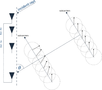
Figure 3: Phase change across subcarriers with distance.

Algorithm 2 MUSIC Procedure for Estimating $\rho$

Calculate the CSI across antennas and subcarriers covariance matrix ${\bf R}$ = $\mathbb{E}[{\bf h}{\bf h}^{H}]$

Get the eigenvectors and eigenvalues of R

Separate system subspace $\cal S$ and noise subspace $\cal N$ by defining a threshold

Calculate ${\bf N}$ by concatenating the eigenvectors of $\cal N$

for $\rho=0:1000$ in increments of 1 do

  Calculate vector ${\bf B}(\rho)$

  Calculate the $\textrm{PMF}(\rho)=\frac{1}{\textrm{Norm}_{2}({\bf N}^{H}{\bf B}(\rho))}$

end for

Search the PMF for a peak and find the corresponding $\rho$

For this algorithm, we use the same principle for estimating $\rho$ as in estimating $\theta$. We assume the transmission is multicarrier-based, and we use MUSIC to make use the phase difference among subcarriers. Please refer to Fig. 3. Note that as the ray travels, the phases of the subcarriers change with rate according to their frequencies. If the subcarriers have a spacing of $\Delta\!f$ and we have $N_{S}$ subcarriers, their phase relation with distance is given as

$${\bf B}(\rho)=(1,e^{-j2\pi\rho\Delta\!{f}/c},e^{-j2\pi\rho 2\Delta\!{f}/c},\ldots,e^{-j2\pi\rho(N_{s}-1)\Delta\!{f}/c})^{T}$$ (6)

where $\rho$ is the distance and $c$ is the speed of light. The vector ${\bf B}(\rho)$ will be used exactly as we used the steering vector ${\bf A}(\theta)$ in estimating $\theta$. The procedure is explained in Algorithm 2. We call the combination of using MUSIC to estimate $\theta$ and using MUSIC to estimate $\rho$ the MUSIC/MUSIC (MM) algorithm.

IV Simulation Environment and Basis for Comparison

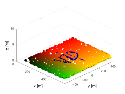
Figure 4: 3D environment.

We employed the simulation environment in [1] with the purpose of comparing the performance in a fair fashion, as in [2]. The simulation parameters we used are given in Table I at SNR = 0 dB. SNR is defined as the ratio of the signal power to the noise power and 0 dB means that the two are equal. We used a three-dimensional environment exactly as in paper [1] as shown in Fig. 4, where the antenna is 8.5 meters above the plane of the UEs. The simulation environment is 1000m $\times$ 500m. The 2048 UEs are placed randomly, except 234 of the UEs are selected to make the word “VIP,” so we can see if the channel chart preserves the shape.

In addition to a visual comparison of channel charts, we will use continuity (CT) and trustworthiness (TW) as objective performance measures [1, 2]. CT specifies if neighbors in the original space are close in the representation space. TW measures how well the feature mapping avoids introducing new neighbor relations that were not present in the original space. For mathematical descriptions of point-wise and global CT and TW, we refer the reader to [1, 2] Point-wise and global CT and TW are between 0 and 1, with larger values being better [1].

V Algorithms for AoA Estimation

We will discuss three relatively simple algorithms on AoA estimation from the literature. For an introduction to this subject, see, e.g., [10, 11].

V-A Bartlett’s Algorithm

With our earlier definition of the autocorrelation matrix ${\bf R}$ and the steering vector $A(\theta)$, this algorithm computes

$$P_{\it Bartlett}(\theta)=\frac{{\bf A}^{H}(\theta){\bf R}{\bf A}(\theta)}{{\bf A}^{H}(\theta){\bf A}(\theta)}$$ (7)

and then finds the maximum of $P_{\it Bartlett}(\theta)$. For a ULA, the denominator is a constant, and it is sufficient to work with

$$P_{\it Bartlett}(\theta)={\bf A}^{H}(\theta){\bf R}{\bf A}(\theta).$$ (8)

For a derivation of this algorithm via optimization, see, e.g., [11].

V-B MVDR (Capon’s) Algorithm

The full name for this algorithm is Minimum Variance Distortionless Algorithm (MVDR). It is also know as Capon’s algorithm. Its spatial spectrum $P_{\it MVDR}(\theta)$, similar to $P_{\it Bartlett}(\theta)$, is given as

$$P_{\it MVDR}(\theta)=\frac{1}{{\bf A}^{H}(\theta){\bf R}^{-1}{\bf A}(\theta)}.$$ (9)

Once again, after calculation, one searches for the maximum of $P_{\it MVDR}(\theta)$ to determine the AoA.

V-C Minimum Norm Algorithm

This algorithm carries out an eigenspace analysis as in MUSIC. It performs the eigenvalue decomposition

$${\bf R}={\bf U}\boldsymbol{\Sigma}{\bf U}^{H}=\left[{\bf U}_{s}\ \;{\bf U}_{n}\right]\left[\begin{array}[]{cc}{\bf D}_{s}&{\bf 0}\\ {\bf 0}&\sigma^{2}{\bf I}\end{array}\right]\left[{\bf U}_{s}\ \;{\bf U}_{n}\right]^{H}$$ (10)

where ${\bf U}_{s}$ corresponds to the signal subspace, consisting of $K$ signal eigenvectors; ${\bf U}_{n}$ corresponds to the noise subspace, consisting of $N-K$ noise eigenvectors; ${\bf D}_{s}$ is a $K\times K$ diagonal matrix with signal eigenvalues as the entries; and ${\bf I}$ is an $(N-K)\times(N-K)$ identity matrix. Then, the Minimum Norm Algorithm computes the spatial spectrum as

$$P_{\it MinNorm}(\theta)=\frac{1}{{\bf A}^{H}(\theta){\bf U}_{n}{\bf U}_{n}^{H}{\bf e}{\bf e}^{H}{\bf U}_{n}{\bf U}_{n}^{H}{\bf A}(\theta)}$$ (11)

where ${\bf e}$ is the first column of the identity matrix of size $N\times N$.

VI Simulation Results

We will first consider the ability of the Bartlett, MVDR, and Minimum Norm AoA algorithms to estimate $\theta$ and one of LR, ISQ, and MUSIC algorithms to estimate $\rho$. The results in terms of channel charts are given in Figs 5-7. Based on these charts, one can state that for any of Bartlett, MVDR, and Minimum Norm algorithms for estimating $\theta$, the MUSIC algorithm to estimate $\theta$ appears to be the best, while the LR and ISQ algorithms not appearing performing much different from each other.

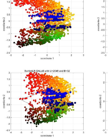
Figure 5: Channel charts with Bartlett algorithm for $\theta$ and LR (left column), ISQ (middle column), and MUSIC (right column) algorithms for $\rho$ for the 3D LOS (top row), QLOS (middle row), and QNLOS (bottom row) channels.

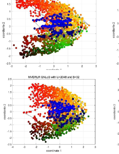
Figure 6: Channel charts with MVDR algorithm for $\theta$ and LR (left column), ISQ (middle column), and MUSIC (right column) algorithms for $\rho$ for the 3D LOS (top row), QLOS (middle row), and QNLOS (bottom row) channels.

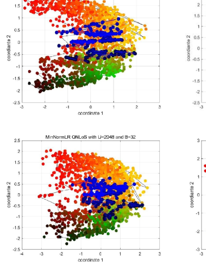
Figure 7: Channel charts with Minimum Norm algorithm for $\theta$ and LR (left column), ISQ (middle column), and MUSIC (right column) algorithms for $\rho$ for the 3D LOS (top row), QLOS (middle row), and QNLOS (bottom row) channels.

On the other hand, Table II tabulates the execution runtimes of the algorithms in Fig. 5–7. According to this table, the execution times of MUSIC for $\theta$ are much larger than those of LR and ISQ. It can be seen that in execution times, using MUSIC for estimating $\rho$ causes a large runtime, while using LR or ISQ have similar runtimes. On the other hand, among Bartlett, MVDR, and Minimum Norm for estimating $\theta$, Minimum Norm has a very large runtime against Bartlett and MVDR. This means, we can eliminate Minimum Norm from consideration in estimating $\theta$.

TABLE II: Execution runtimes of the algorithms in Figs. 5–7. The units are in seconds. The results are the averages of three runs.

	Bartlett/LR	Bartlett/ISQ	Bartlett/MUSIC
LoS	0.4212	0.4154	16.0008
QLoS	0.4330	0.4113	15.9934
QNLoS	0.4789	0.4679	15.8993
	MVDR/LR	MVDR/ISQ	MVDR/MUSIC
LoS	6.4927	6.3431	21.0445
QLoS	6.4952	6.4381	21.2382
QNLoS	6.4735	6.4374	21.2727
	Min. Norm/LR	Min. Norm/ISQ	Min. Norm/MUSIC
LoS	13.5298	13.1709	28.1667
QLoS	12.8640	13.1466	27.7734
QNLoS	13.0934	13.0816	28.0243

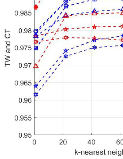
Figure 8: TW and CT values for an LOS channel.

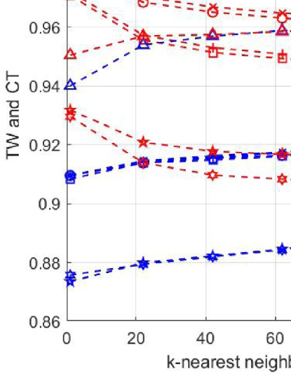
Figure 9: TW and CT values for a QLOS channel.

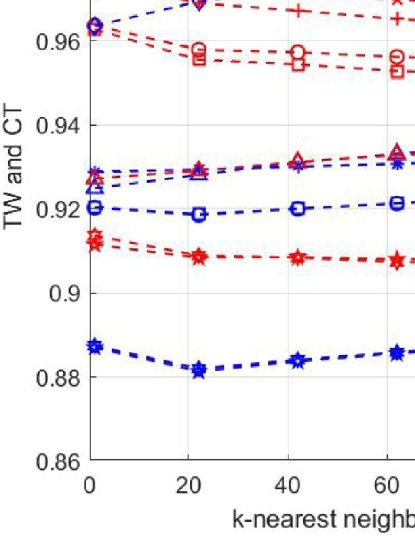
Figure 10: TW and CT values for a QNLOS channel.

We tabulate the TW and CT values of the algorithms in Figs. 5–7 for LOS, QLOS, and QNLOS channels at 102 nearest points in Table III. Since we have already eliminated Minimum Norm algorithm, we conclude from this table that the Bartlett algorithm may have an edge over the MVDR algorithm in terms of TW and CT performance. To investigate this further, we consider Figs. 8–10 in LOS, QLOS, and QNLOS channels for $k$ nearest neighbors for values of $k$ in the range 0–102. A careful study of these plots indicate that, in terms of TW and CT performance, Bartlett algorithm can indeed be a contender even though it can be implemented in a simple fashion.

TABLE III: TW and CT values of the algorithms in Figs. 5–6 for LOS, QLOS, and QNLOS channels.

Measure	Channel	Bartlett	Bartlett	Bartlett	MVDR/	MVDR/	MVDR/	MinNorm/	MinNorm/	MinNorm/
		LR	ISQ	MUSIC	LR	ISQ	MUSIC	LR	ISQ	MUSIC
TW	LOS	0.9930	0.9885	0.9998	0.9796	0.9753	0.9864	0.9330	0.9885	0.9998
	QLOS	0.9203	0.9205	0.9975	0.8882	0.8889	0.9607	0.9192	0.9194	0.9960
	QNLOS	0.9322	0.9324	0.9857	0.8887	0.8898	0.9362	0.9234	0.9238	0.9769
CT	LOS	0.9968	0.9940	0.9998	0.9816	0.9761	0.9864	0.9968	0.9940	0.9998
	QLOS	0.9622	0.9483	0.9989	0.9158	0.9068	0.9601	0.9606	0.9468	0.9974
	QNLOS	0.9682	0.9631	0.9872	0.9082	0.9067	0.9354	0.9552	0.9513	0.9773

In our work [2], we came to the conclusion that using the MUSIC algorithm for estimating both $\theta$ and $\rho$ among the algorithms studied in that paper, including LR and ISQ. We call the resulting algorithm MUSIC/MUSIC, or MM. We show the performance of employing the MM algorithm in Fig. 11. In Table V we provide TW and CT values at 102 nearest points using the MM algorithm. We provide the running times of using the MM algorithm in Table V.

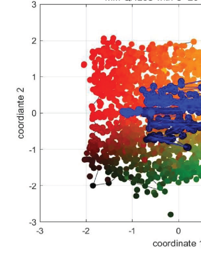
Figure 11: Channel charts and TW and CT values for employing the MUSIC algorithm to estimate both $\theta$ and $\rho$.

TABLE IV: TW and CT values at 102 nearest points for employing the MUSIC algorithm to estimate both $\theta$ and $\rho$.

Measure	Channel	MUSIC/MUSIC
TW	LOS	0.9998
	QLOS	0.9975
	QNLOS	0.9854
CT	LOS	0.9998
	QLOS	0.9989
	QNLOS	0.9867

TABLE V: Running times for employing the MUSIC algorithm to estimate both $\theta$ and $\rho$.

Channel	Runtime (s)
LOS	20.6577
QLOS	20.6061
QNLOS	20.8503

We show the performance of employing the Bartlett algorithm for estimation of both $\theta$ and $\rho$ in Fig. 12. In Table VII we provide TW and CT values at 102 nearest points using Bartlett algorithm for both $\theta$ and $\rho$. We provide the running times of using the Bartlett algorithm to estimate both $\theta$ and $\rho$ in Table VII. In implementing the Bartlett algorithm, Cholesky factorization of the autocorrelation matrix ${\bf R}$ is made for reduction in computational complexity. From the results presented, clearly the Bartlett algorithm has a substantial reduction in computational complexity without a discernible reduction in the quality of the channel charts or performance measures TW and CT.

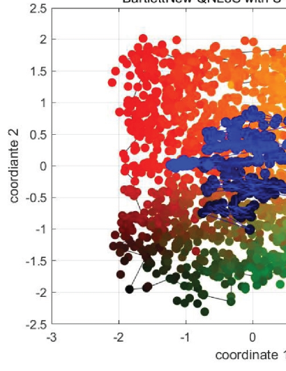
Figure 12: Channel charts and TW and CT values for employing the Bartlett algorithm to estimate both $\theta$ and $\rho$.

TABLE VI: TW and CT values at 102 nearest points for employing the Bartlett algorithm to estimate both $\theta$ and $\rho$.

Measure	Channel	Bartlett/Bartlett
TW	LOS	0.9998
	QLOS	0.9974
	QNLOS	0.9871
CT	LOS	0.9998
	QLOS	0.9988
	QNLOS	0.9892

TABLE VII: Running times for employing the Bartlett algorithm to estimate both $\theta$ and $\rho$.

Channel	Runtime (s)
LOS	1.1203
QLOS	1.1407
QNLOS	1.1373

VII Conclusion

The LR, ISQ, and MM algorithms we presented in [2] significantly outperformed the three algorithms in the seminal paper [1], PCA, SM, and AE, in terms of performance. In this paper, we investigated the performance of the more conventional AoA estimation algorithms Bartlett, Minimum Variance Distortion Response (MVDR or Capon), and Minimum Norm algorithms. As in [1], we measured the performance in terms of the visual appearance of the channel charts, as well as connectivity (CT) and trustworthiness (TW). We also considered execution time or running time of the algorithms. In our study of the use of the MUSIC algorithm to estimate $\theta$ and one of Bartlett, MVDR, or Minimum Norm algorithms, we conclude that all three conventional algorithms can be competitive.

References

- [1] C. Studer, S. Medjkouh, E. Gonultas, T. Goldstein, and O. Tirkkonen, “Channel charting: Locating users within the radio environment using channel state information,” IEEE Access, vol. 6, pp. 47 682–47 698, 2018.
- [2] A. Aly and E. Ayanoglu, “Model-based approaches to channel charting,” IEEE Transactions on Communications, vol. 72, no. 2, pp. 1207–1222, Feb. 2024.
- [3] ——, “Estimation of cellular wireless user coordinates via channel charting and MUSIC,” in 2023 International Conference on Computing, Networking and Communications (ICNC), 2023, pp. 343–347.
- [4] ——, “Channel charting: Model-based approaches,” in ICC 2023 - IEEE International Conference on Communications, 2023, pp. 1054–1060.
- [5] S. Jaeckel, L. Raschkowski, K. Borner, and L. Thiele, “Quadriga: A 3-D multi-cell channel model with time evolution for enabling virtual field trials,” IEEE Trans. Antennas Propag., vol. 62, no. 6, pp. 3242–3256, 2014.
- [6] “Quadriga: The next generation radio channel model,” https://quadriga-channel-model.de/.
- [7] S. Jaeckel, “Quasi-deterministic channel modeling and experimental validation in cooperative and massive MIMO deployment topologies,” Ph.D. dissertation, Technische Universitat Ilmenau, 2016.
- [8] L. L. Magoarou, T. Yassine, S. Paquelet, and M. Crussiere, “Channel charting based beamforming,” in 2022 56th Asilomar Conference on Signals, Systems, and Computers, 2022, pp. 1185–1189.
- [9] C. Studer, E. Gonultas, and S. Medjkouh, “Simple channel charting MATLAB simulator,” https://github.com/IIP-Group/ChannelCharting.
- [10] H. L. Van Trees, Optimum Array Processing: Part IV of Detection, Estimation, and Modulation Theory. Wiley, 2002.
- [11] H. Krim and M. Viberg, “Two decades of array signal processing research: The parametric approach,” IEEE Signal Processing Magazine, vol. 13, no. 4, pp. 67–94, 1996.