An introduction to reservoir computing

Abstract

There is a growing interest in the development of artificial neural networks that are implemented in a physical system. A major challenge in this context is that these networks are difficult to train since training here would require a change of physical parameters rather than simply of coefficients in a computer program. For this reason, reservoir computing, where one employs high-dimensional recurrent networks and trains only the final layer, is widely used in this context. In this chapter, I introduce the basic concepts of reservoir computing. Moreover, I present some important physical implementations coming from electronics, photonics, spintronics, mechanics, and biology. Finally, I provide a brief discussion of quantum reservoir computing.

This book chapter will appear in: M. te Vrugt (Ed.), Artificial Intelligence and Intelligent Matter, Springer, Cham (2025)

1 Introduction

You know that it is possible to perform machine learning tasks on a computer, but did you know that it is also possible to do so with a bucket of water? Precisely that was demonstrated in Ref. Fernando and Sojakka (2003). Input data was mechanically fed into a bucket, recordings of the water surface then could be used for classification tasks. This is a form of reservoir computing (RC), which this chapter will provide an introduction to.

The core idea of RC is that a significant portion of the computing task is performed not by a trained network, but by a very high-dimensional system (reservoir) that is essentially treated as a black box and whose output is fed into a single readout layer, which is the only component of the network that is trained. This setup is illustrated in Fig. 1. Since physical systems are generally much more difficult to train than neural networks on a computer, RC is a very promising approach for implementing artificial intelligence in a physical system (for example a bucket of water or – more relevant in practice – optical or magnetic systems). Consequently, RC has attracted considerable interest among physicists in recent years. From a computer science point of view, on the other hand, RC is useful for the otherwise difficult task of training recurrent neural networks.

The foundations of what is nowadays referred to as reservoir computing were independently developed by Jaeger (2001), who referred to it as echo state network, and by Maass et al. (2002), who called it liquid state machine. (There were some earlier ideas in this direction – see Refs. Kirby and Day (1990); Kirby (1991); Schomaker (1991) – that are largely unknown today Nakajima and Fischer (2021).) The name “reservoir computing” was coined in Refs. Verstraeten et al. (2005, 2007) to unify these concepts. RCs are particularly useful for tasks involving some temporal dynamics without needing external memory, since what they do depends also on the value of the input signal at previous times. Reviews of RC can be found in Refs. Lukoševičius and Jaeger (2009); Van der Sande et al. (2017); Cucchi et al. (2022); Lukoševičius et al. (2012); Everschor-Sitte et al. (2024), a book on the topic was edited by Nakajima and Fischer (2021).

2 Basic concepts of reservoir computing

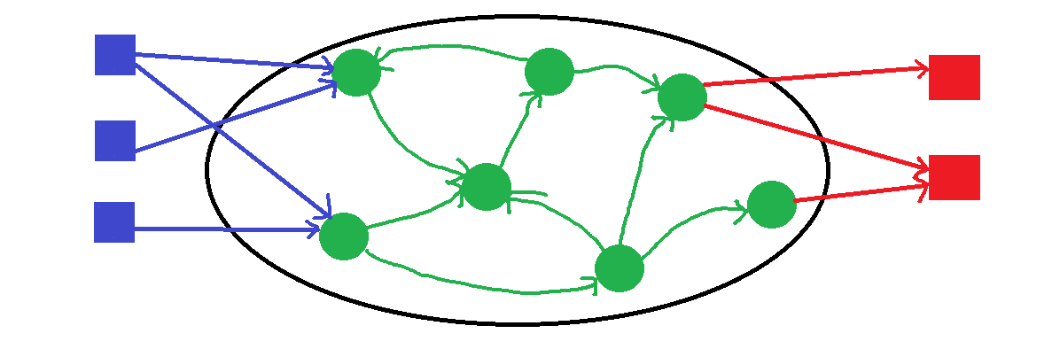
Figure 1: Illustration of the basic framework of reservoir computing. The input (blue) is fed into a recurrent neural network (green) and subsequently into an output layer (red). (A similar figure can be found in Ref. Van der Sande et al. (2017).)

2.1 How reservoir computing works

The discussion follows Refs. Cucchi et al. (2022); Mujal et al. (2021) (and also adapts the notation used there).

Suppose that we have an $n$-dimensional training input signal $\vec{u}_{\mathrm{train}}(t)$ (depending on time $t$) that is supposed to lead to a certain $m$-dimensional output signal $\vec{y}_{\mathrm{train}}(t)$. For instance, if the system is supposed to predict time series data, $\vec{u}_{\mathrm{train}}(t)$ would be the first part of a time series and $\vec{y}_{\mathrm{train}}(t)$ the second part (that we want to predict from the first part) Cucchi et al. (2022). The input signal is used to drive a high-dimensional nonlinear dynamical system that is referred to as the reservoir.

Specifically, the state $\vec{X}$ of the reservoir at time $t_{i}$ takes the form Mujal et al. (2021)

$$\vec{X}(t_{i})=\vec{f}(\vec{X}(t_{i-1}),\vec{u}(t_{i}))$$ (1)

with the input signal $\vec{u}$ and a function $\vec{f}$. A sufficiently large subset of the state variables, summarized in a vector $\vec{x}(t)$, must be accessible. Finally, a readout function $\vec{F}$ maps the vector $\vec{x}(t)$ to the output $\vec{y}(t)$, i.e.,

$$\vec{F}(\vec{x}(t))=\vec{y}(t).$$ (2)

This readout function is the only thing that is touched during the training process. It is designed to minimize a loss function that typically that depends on the difference between the actual output $\vec{y}(t)$ and the desired output $\vec{y}_{\mathrm{train}}(t)$. In most cases, $\vec{F}$ is obtained via linear regression. Once $\vec{F}$ is known, one can apply the system to new input signals $\vec{u}(t)$.

This strategy has a number of advantages:

• The training usually only consists in linear regression, which is simple, computationally inexpensive, and easy to implement.

• One only needs to train the readout function $\vec{F}$ and not the entire system. This is helpful if we are dealing with a physical system where the precise interactions between the parts are difficult to modify and perhaps not even fully known.

• One can use the same reservoir for different computing tasks by simply using different readout functions $\vec{F}$.

• It is a good approach for dealing with time series data.

Almost every physical system can be described by an equation of the form (1), and therefore a large variety of physical system can be used as reservoirs (although in practice there are restrictions, see Section 3). A notable feature of RCs is their temporal dynamics. Iterating Eq. (1) gives Mujal et al. (2021)

$$\vec{X}(t_{i})=\vec{f}(\vec{f}(\vec{f}(\vec{X}(t_{i-3}),\vec{u}(t_{i-2})),\vec{u}(t_{i-1})),\vec{u}(t_{i})),$$ (3)

showing that the system’s state at a certain time depends on the system states and inputs at previous times. This allows the system to react to temporal input signals, such as spoken language.

2.2 Recurrent neural networks

An essential distinction in this context (see also the chapter by Tobias Wand in this volume) is that between a feed-forward neural network (FNN) and a recurrent neural network (RNN). In a FNN, signals propagate in one direction - the first layer activates the second layer, the second layer the third layer and so on. In a RNN, on the other hand, information can also “move backwards”. This allows the system to have memory: If a system is supposed to process a signal $\vec{u}(t)$, then reacting to $\vec{u}(t_{2})$ might require also information about $\vec{u}(t_{1})$ with $t_{1}<t_{2}$. This can be achieved by feeding back information about previous states of nodes. This distinguishes RC from the related concept of an extreme learning machine Huang et al. (2015); Wang et al. (2022), which employs FNNs and do therefore not have memory of this type Butcher et al. (2013).

The existence of closed loops implies in particular that RNNs can have a temporal dynamics even in the absence of external inputs. Therefore, while FNNs are (mathematically speaking) functions – they map a certain input to a certain output – RNNs are (mathematically speaking) dynamical systems Lukoševičius and Jaeger (2009). This already indicates how they might be related to RC, which, as discussed in Section 2.1, is based on dynamical systems. Frequently, in computer science applications, the dynamical system constituting the reservoir is a RNN.

In general, RNNs are difficult to train. FNNs are typically trained via gradient descent methods, where the parameters giving the connection weights are gradually changed to move the network’s output closer to the target output. Gradient descent methods are also frequently, and in many different forms, applied to RNNs Atiya and Parlos (2000). However, such methods are considerably more difficult to apply in the context of RNNs. Reasons for this include that a gradual parameter change might lead to a bifurcation that spoils convergence and that training times are very long since a single parameter change requires running the temperal dynamics for some time. RC was proposed as a new method for training RNNs that allows to avoid these problems by changing the weights only in a non-recurrent readout layer. The RNN itself can be created randomly and is unchanged during the training Lukoševičius and Jaeger (2009).

2.3 Why does this work?

At first sight, the idea of RC is somewhat counterintuitive. While it is of course easier to train only the final layer of a neural network rather than the entire one, there is certainly a reason why one usually trains all layers. Usually one would not get away with only changing the final layer, so why is it possible here?

What is exploited here is the high dimensionality of the reservoir. The information that we are interested in is in principle encoded in the input signal, but it is mixed up, nonlinearly, with a huge amount of other stuff that we are not interested in. The projection onto a higher-dimensional space allows for separability. This idea is illustrated in Fig. 2. Suppose we want to classify some inputs into stars and circles. Unfortunately, due to the way the data is distributed, it does not exhibit linear separability, i.e., we cannot find a hyperplane (in this case a line) that gives us the border between a region with stars and a region with circles (cf. Fig. 2a). If, however, we project the data onto a three-dimensional space (cf. Fig. 2b), we can find a hyperplane (in this case a plane) that separates stars and circles. The separation problem has thereby become much simpler, and can be solved already by a single layer that is trained via linear regression. In RC, feeding the data into the reservoir corresponds to the projection from the two- to the three-dimensional plane (usually more dimensions will be involved) and the training of the readout layer corresponds to finding the plane Seoane (2019).

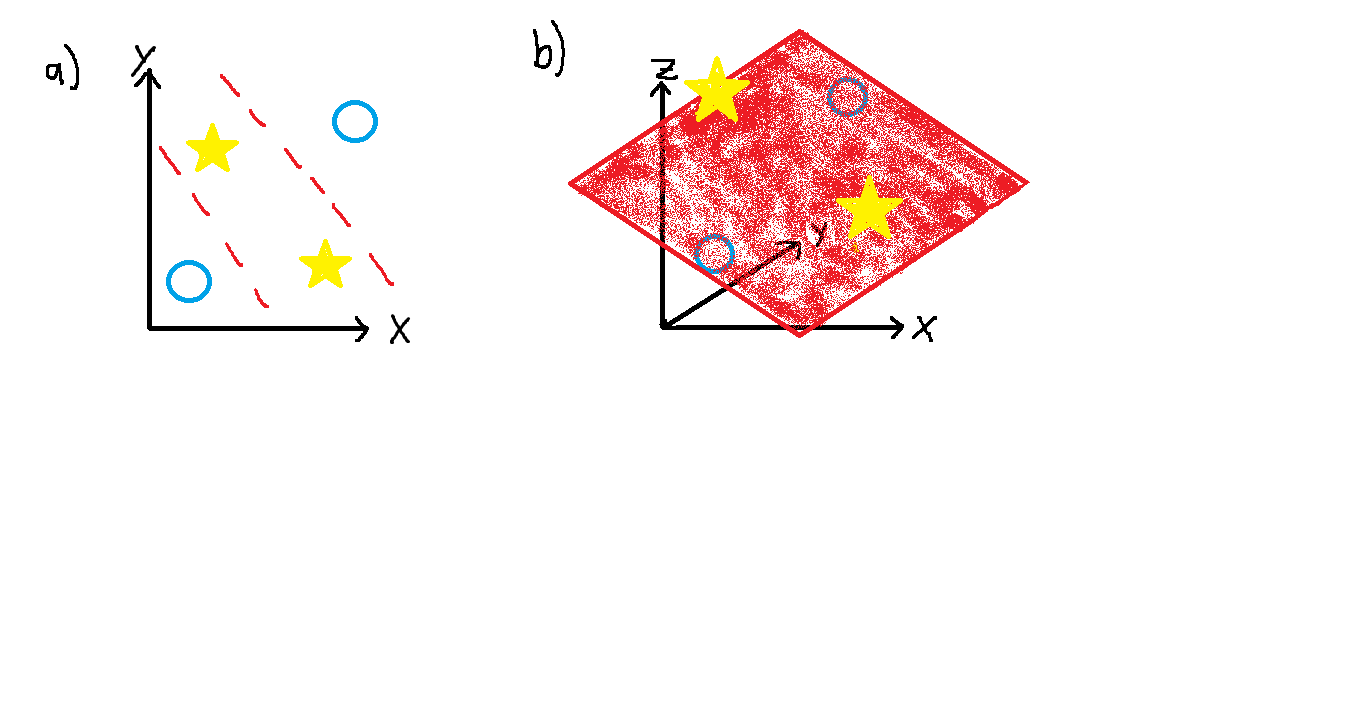
Figure 2: Projection onto a high-dimensional space allows for separability. (A similar figure can be found in Ref. Appeltant et al. (2011).)

3 What is a good reservoir?

While the procedure discussed above can in principle be applied very generally, not every dynamical system does in practice make a good reservoir. A number of criteria have been developed that a reservoir should satisfy to be useful in this context – although the broad range of systems that have been used for this purpose (consider, for example, the water bucket mentioned above) suggests that in practice these criteria are quite flexible Seoane (2019).

First, reproducibility is of course important. If two input signals are very similar, the output signals should be similar as well. This is related to the ability of the system to generalize from the data it has been trained on to other input data Seoane (2019). Second, if the input signals are sufficiently different, the output signals should also be different (separation). This determines the reservoir’s ability to distinguish different sorts of inputs. A reservoir computer that always produces the same output regardless of the input obviously satisfies the reproducibility property, but would not be really useful.

Moreover, fading memory is an important property of reservoir computers Cucchi et al. (2022). The computer is supposed to process a time series $\vec{u}(t)$, not just he instantaneous value of $\vec{u}$ (the latter would not require a RNN). Therefore, it needs to have memory. On the other hand, the current value of $\vec{u}$ should still be what is most important, values at earlier times become gradually less important. In other words, the memory should gradually fade. The computer should relax to a quiescent state if there is no external input Van der Sande et al. (2017), and its behavior should not depend on the initial condition $\vec{X}(0)$ of the reservoir. This is referred to as the echo state property - the influence of initial conditions should gradually vanish Yildiz et al. (2012). The timescale of the fading memory should be comparable to the timescales of the input signal Kaspar et al. (2021). Since it depends on the application what the timescale of the input signal is, the adequate reservoir system may differ depending on the application.

Also, it is often considered advantageous to operate the reservoir computer in a parameter range close to an instability (for example, in the vicinity of a transition to chaos), since there its behavior is particularly complex and therefore has a very high computational complexity. Intuitively, the reason is that such regimes present a compromise between ordered phases (where the behavior is stable and thus reliable, but where initial conditions are also quickly erased by the approach to an attractor making the system less able to react to an input) and chaotic phases (where the system’s behavior is strongly affected by small differences in the initial conditions, harming separability) Seoane (2019). There are, however, also counterexamples, i.e., systems where moving close to an instability actually decreases the performance of a reservoir computer Carroll (2020). In fact, Herbert Jaeger (in his foreword for Ref. Nakajima and Fischer (2021)) argues that the idea that RC should operate close to chaos or criticality is a “myth”, neither mathematically well-defined nor empirically confirmed.

4 Physical reservoir computing

The discussions so far were concerned with general concepts in artificial intelligence. This book, however, has a specific focus on the relation of AI to physics, and there is a reason that RC features so prominently in the introductory part of this book. This reason is physical reservoir computing.

In physical RC, the reservoir is a physical system. Thereby, physical RC allows to perform machine learning tasks using physical systems. There has, in recent years, been a considerable amount of work on the development of experimental setups that can be used for this purpose. In this section, I will briefly discuss some examples. Later chapters will address specific such as in optics (in the chapter by Kathy Lüdge/Lina Jaurigue), spintronics (in the chapter by Atreya Majumdar/Karin Everschor-Sitte), and soft matter (in the chapter by Julian Jeggle/Raphael Wittkowski). The classification in different types of reservoirs (electronic, photonic, spintronic, mechanical, biological, chemical) is adapted from Ref. Tanaka et al. (2019). Note that this list is not exhaustive.

4.1 Electronic reservoir computing

Standard computers are based on electronics, and therefore it is a very natural idea to use electronic systems. This has been achieved in a broad number of ways (see Refs. Tanaka et al. (2019); Liang et al. (2024) for an overview), of which I discuss here just one, namely memristors. A memristor is a resistor that possesses memory, i.e., whose resistance changes based on the current that has passed through it. Memristors are therefore useful devices in applications like RC where memory is important. They can be used to mimic the plasticity of biological neurons, and allow for nonlinear transformations of input signals Tanaka et al. (2019). A memristor-based RC was first proposed by Kulkarni and Teuscher (2012).

4.2 Photonic reservoir computing

In photonics, information processing is based not (solely) on electric currents, but on light (photons). RC has developed into a widely used approach in photonics, see Ref. Van der Sande et al. (2017) for a review (I am loosely following this reference here). An important approach is the implementation of RC in on-chip-photonics, where photonic systems are integrated into chips. This allows the systems to be produced and sold on industrial scales and to therefore use them for high-speed low-power-consumption computing. This approach was theoretically suggested in Ref. Vandoorne et al. (2008) and later realized in hardware Vandoorne et al. (2014).

A further interesting approach is delay reservoir computing Hülser et al. (2022). Delay systems have been of considerable interest for optics in the past years Seidel et al. (2022); Koch et al. (2023). They are described mathematically by delay differential equations, which differ considerably from ordinary differential equations since they possess an infinite-dimensional phase space – for solving it, one needs to specify not only the state of the system at a single initial time, but on an entire time interval. Using delay systems, one can therefore achieve a high-dimensional phase space (which is advantageous in the context of RC) even with a very simple setup Van der Sande et al. (2017).

Photonic approaches to neuromorphic computing are discussed further in the chapters by Kathy Lüdge/Lina Jaurigue and by Lennart Meyer/Rongyang Xu/Wolfram Pernice in this book.

4.3 Spintronic reservoir computing

Spintronics is a field of technology where information processing is based not only on the electric charges (as in electronics), but also on the spins (elementary magnetic moments) of electrons. Spintronics has become increasingly popular in neuromorphic computing in general and RC in particular, see Refs. Zhou and Chen (2021); Finocchio et al. (2021); Grollier et al. (2020); Everschor-Sitte et al. (2024); Yan et al. (2024); Liang et al. (2024) for reviews. Spintronic systems can be used to build artificial synapses, thereby mimicking the structure and functionality of biological brains Grollier et al. (2020). An introduction is provided in the chapter by Atreya Majumdar/Karin Everschor-Sitte in this book.

An interesting recent proposal in this context is Brownian reservoir computing based on skyrmions Raab et al. (2022); Brems et al. (2021, 2023a, 2023b). Brownian motion Brown (1828) is the random thermal motion of particles, which is a central phenomenon in soft matter physics, but also arises in magnetic systems. An example are magnetic skyrmions, which are whirl-like topological magnetic nanostructures that have particle-like diffusion behavior reminiscent of neurotransmitters and can be used as information carriers in spintronics Grollier et al. (2020). In Brownian computing, one employs thermal fluctuations – which in most systems are present anyway – for computing purposes to achieve a high energy efficiency. It is of course helpful if the employed Brownian system can be easily integrated into a computer, which is why magnetic nanosystems such as skyrmions are useful here Brems et al. (2023a). Brownian RC based on skyrmions was realized experimentally by Raab et al. (2022), who demonstrated that this approach is very promising for energy-efficient computing.

4.4 Mechanical reservoir computing

Mechanical systems can make for useful reservoirs. Robotic systems, in particular from soft robotics (where the bodies of the robots are flexible), have been repeatedly used in this context. Hauser et al. (2011) have modeled this using the example of a nonlinear mass-spring-damper system connected to a mechanical network, which was intended to represent in a simple way the body of a soft robot (or biological system) and which exhibits the complex nonlinear dynamics required for successful RC. Nakajima et al. (2014) employed a silicon-based robot arm inspired by the arm of an octopus, with the input being the rotation of the arm and the output being measured strain. While the noisy and nonlinear dynamics of soft robots is often perceived as disadvantageous, it can be very useful in the context of RC. (This paragraph follows Ref. Hauser (2021).)

4.5 Biological and chemical reservoir computing

Reservoir computing has always had a close connection to neurobiology. In particular, work on RC has been motivated by attempts to understand information processing in mammalian brains Sumi et al. (2023). For instance, it has been proposed that the cerebellum might work like a liquid state machine Yamazaki and Tanaka (2007), and experiments on mice Cazettes et al. (2023) suggest that the mouse brain exploits principles of RC Cazettes et al. (2023); Liang et al. (2024). Moreover, RC – which is frequently based on random neural networks and noisy systems – might explain why the brain works so accurately despite being a rather noisy system Lukoševičius and Jaeger (2009). It is therefore a promising direction of work to use biological neural networks for RC tasks Sumi et al. (2023). Biological neurons are in a sense the most obvious, but not the only approach to biological RC. For example, it has been proposed to realize RC based on Escherichia coli bacteria Jones et al. (2007). Another variant, namely DNA reservoir computing Goudarzi et al. (2013), will be discussed in the chapter on DNA neural networks in this book. This approach is based on employing chemical systems for RC, an idea that is also used in non-biological contexts (for example based on electrolyte solutions Kan et al. (2021)). See the chapter by Julian Jeggle/Raphael Wittkowski in this volume for a discussion of the related concept of active matter RC.

5 Quantum reservoir computing

In the wake of the currently growing interest in quantum computing in general and quantum-mechanical approaches to machine learning in particular, quantum reservoir computing Fujii and Nakajima (2017); Martínez-Peña et al. (2021); Fujii and Nakajima (2021); Suzuki et al. (2022); Mujal et al. (2021) has attracted some interest. Here, one employs quantum-mechanical reservoirs and thereby aims to exploit the advantages of quantum computers for RC. In this section, I will introduce the elementary ideas of how this works. The discussion follows Ref. Fujii and Nakajima (2017), which was one of the first articles on this topic. A more general introduction to quantum machine learning can be found in the chapter by Ivana Nikoloska in this volume.

Quantum states are represented by vectors in complex Hilbert states. In the context of quantum computing, the minimal information unit is a qubit, corresponding to a two-dimensional complex vector in a vector space spanned by the vectors $\ket{0}$ and $\ket{1}$. In general, the state of a system of $N$ qubits is described by a $2^{N}x2^{N}$ Hermitian matrix $\rho$, the density matrix. The quantum system is said to be in a pure state if $\rho$ can be written as $\rho=\ket{\psi}\bra{\psi}$, where $\ket{\psi}$ is a $2^{N}$-dimensional vector and $\bra{\psi}$ is a covector to $\ket{\psi}$. (For instance, if $\ket{\psi}=(1,2,3)^{\mathrm{T}}$, then $\bra{\psi}=(1,2,3)$.) If the density matrix at time $t$ is $\rho(t)$, then the density matrix at time $t+\tau$ is

$$\rho(t+\tau)=e^{-\mathrm{i}H\tau}\rho(t)e^{\mathrm{i}H\tau}$$ (4)

with the Hamiltonian $H$ (a $2^{N}x2^{N}$ Hermitian matrix that determines the dynamics and whose eigenvalues correspond to the energy levels of the quantum system). For an arbitrary observable $A_{i}$, which is also represented by a $2^{N}x2^{N}$ Hermitian matrix, the expectation value is given by

$$a_{i}(t)=\operatorname{Tr}(\rho(t)A_{i})$$ (5)

with the trace $\operatorname{Tr}$.

What is now required is a way to feed an input signal $\vec{u}(t)$ into the system and to get an output signal $\vec{x}(t)$ that can then be fed into the readout function $\vec{F}$. Let us consider for simplicity a one-dimensional input signal $u(t)$, which we sample in $M$ discrete time intervals of length $\tau$ to get a sequence $\{u_{k}\}$ with $u_{k}=u(k\tau)$ and $k=0,1,...M$. At each time $k\tau$, the state of the first qubit is changed to $\rho_{u_{k}}=\ket{\psi_{u_{k}}}\bra{\psi_{u_{k}}}$ with

$$\ket{\psi_{u_{k}}}=\sqrt{1-u_{k}}\ket{0}+\sqrt{u_{k}}\ket{1}.$$ (6)

The density matrix $\rho$ is thereby replaced by

$$\rho_{u_{k}}\otimes\operatorname{Tr}_{1}(\rho),$$ (7)

where $\otimes$ is a tensor product and $\operatorname{Tr}_{1}$ is a trace over the degrees of freedom of the first qubit. Afterwards, the density matrix is time evolved via Eq. (4) for a time $\tau$. This time has to be optimized in order to optimize the performance of the computer (see Ref. Fujii and Nakajima (2017)). For the output $\vec{x}(t)$, we then pick some observables $A_{i}$ and assemble them in a vector $\vec{A}$. Then, we can obtain the output vector from their expectation values as

$$\vec{x}(t)=\operatorname{Tr}(\rho(t)\vec{A}).$$ (8)

Specifically, Fujii and Nakajima (2017) choose $A_{i}$ as the Pauli operator acting on the $i$th qubit.

The dimension of the quantum-mechanical Hilbert space increases exponentially with the number of qubits $N$, giving rise to an exponentially increasing number of nodes in the reservoir. For readout purposes, these are split into true nodes (the observed ones) and hidden nodes (the rest). The signals are sampled not only at the time $k\tau$, but also at several times in between. Dividing the time interval into $V$ parts gives rise to $V$ virtual nodes and allows to increase the number of nodes from $N$ to $NV$ via temporal multiplexing. Thereby, the exponentially large Hilbert space is monitored via a polynomial number of signals. This is the distinguishing feature of quantum RC compared to other RC approaches Fujii and Nakajima (2017). Changing $\tau$ corresponds to a change of the dynamics of the reservoir, whereas changing $V$ corresponds to a change of the way it is observed Nakajima et al. (2019).

An important feature of quantum systems is also the way in which they interact with the environment. Such interactions lead to dissipation and decoherence Sannia et al. (2022), where quantum states are destroyed by interactions with the environment. Moreover, performing a measurement of a quantum state generally changes it, a phenomenon giving rise to the famous quantum measurement problem Friebe et al. (2018). Usually, interactions with the environment are not beneficial for the performance of quantum computers. One can, however, also try and exploit such effects in quantum reservoir computing, as has recently been demonstrated for both measurements Mujal et al. (2023) and dissipation Sannia et al. (2022).

6 Outlook: Relation to intelligent matter

If we loosely understand “intelligent matter” as “physical materials perform tasks similar to those expected from computer systems that we would refer to as (artificially) intelligent”, then RC seems to be, if not an instance of it, then at least an important step towards it. We have here physical systems that can be employed in computational tasks of the form that appear in machine learning.

Nevertheless, according to Kaspar et al. (2021), reservoir computing systems in the form described here do not constitute “intelligent matter” in the technical sense:

• The systems possess fading memory, whereas intelligent matter needs to have long-term memory.

• The readout function $\vec{F}$ still needs to be trained manually, the system does not adapt on its own.

Regarding the first point, it should be noted, however, that the fading memory can be tuned to fade rather slowly if this is desired in a certain context.

RC does nevertheless have significant potential for the development of “true” intelligent matter, in particular when considering its relation to evolutionary dynamics (a topic reviewed in Ref. Seoane (2019)). After all, RC is a possible working principle of biological brains. It is conceivable that RC emerges in evolutionary contexts, as it has certain advantages (such as the low cost of learning and the fact that external sytems can be used to carry out computations) that could give biological systems exploiting this paradigm a fitness advantage. An evolutionary evolving RC system would be a system that evolves its computing capabilities in adaptation to the environment, bringing it closer to actual intelligence. A possible disadvantage of RC in evolutionary contexts, Seoane (2019) suggests, is that (since the reservoir needs to be high-dimensional), it requires systems to perform a lot of activity that is not really used for computing, making it energetically costly (which leads to a fitness disadvantage). A fine-tuned neural network can have a smaller number of nodes.

7 Summary

In this chapter, I have introduced the basic ideas of reservoir computing. Here, one uses a very high-dimensional recurrent neural network and trains only the final layer. This makes it possible to use for the rest of the network a physical system whose properties might be difficult to tune or not fully known. A variety of systems have been used here, ranging from buckets of water to optical and magnetic setups. Reservoir computing is a very promising tool for implementing artificial intelligence in nanosystems, and will continue to be a thriving field of research in the coming years.

8 Acknowledgements

I thank Raphael Wittkowski for very helpful discussions on this topic. This work was funded by the Deutsche Forschungsgemeinschaft (DFG, German Research Foundation) in the framework of SFB 1551; Project No. 464588647 and SFB 1552; Project No. 465145163.

References

- Appeltant et al. (2011) Appeltant L, Soriano MC, Van der Sande G, Danckaert J, Massar S, Dambre J, Schrauwen B, Mirasso CR, Fischer I (2011) Information processing using a single dynamical node as complex system. Nature Communications 2(1):468
- Atiya and Parlos (2000) Atiya AF, Parlos AG (2000) New results on recurrent network training: Unifying the algorithms and accelerating convergence. IEEE Transactions on Neural Networks 11(3):697–709
- Brems et al. (2021) Brems MA, Kläui M, Virnau P (2021) Circuits and excitations to enable Brownian token-based computing with skyrmions. Applied Physics Letters 119(13)
- Brems et al. (2023a) Brems MA, Raab K, Virnau P, Kläui M (2023a) Brownscher Reservoir-Computer mit Skyrmionen. Physik in unserer Zeit 54(2):60–61
- Brems et al. (2023b) Brems MA, Raab K, Zázvorka J, Beneke G, Winkle T, Rothörl J, Kammerbauer F, Virnau P, Mentink JH, Kläui M (2023b) Non-conventional computing using thermal and driven skyrmion dynamics. In: 2023 IEEE International Magnetic Conference - Short Papers (INTERMAG Short Papers), pp 1–2, DOI 10.1109/INTERMAGShortPapers58606.2023.10228647
- Brown (1828) Brown R (1828) A brief account of microscopical observations made in the months of June, July and August 1827, on the particles contained in the pollen of plants; and on the general existence of active molecules in organic and inorganic bodies. Philosophical Magazine 4(21):161–173
- Butcher et al. (2013) Butcher JB, Verstraeten D, Schrauwen B, Day CR, Haycock PW (2013) Reservoir computing and extreme learning machines for non-linear time-series data analysis. Neural Networks 38:76–89
- Carroll (2020) Carroll TL (2020) Do reservoir computers work best at the edge of chaos? Chaos: An Interdisciplinary Journal of Nonlinear Science 30(12):121109
- Cazettes et al. (2023) Cazettes F, Mazzucato L, Murakami M, Morais JP, Augusto E, Renart A, Mainen ZF (2023) A reservoir of foraging decision variables in the mouse brain. Nature Neuroscience 26(5):840–849
- Cucchi et al. (2022) Cucchi M, Abreu S, Ciccone G, Brunner D, Kleemann H (2022) Hands-on reservoir computing: a tutorial for practical implementation. Neuromorphic Computing and Engineering 2:032002
- Everschor-Sitte et al. (2024) Everschor-Sitte K, Majumdar A, Wolk K, Meier D (2024) Topological magnetic and ferroelectric systems for reservoir computing. Nature Reviews Physics 6:455–462
- Fernando and Sojakka (2003) Fernando C, Sojakka S (2003) Pattern recognition in a bucket. In: Banzhaf W, Ziegler J, Christaller T, Dittrich P, Kim J (eds) Advances in Artificial Life. ECAL 2003., Berlin, Heidelberg, pp 588–597
- Finocchio et al. (2021) Finocchio G, Di Ventra M, Camsari KY, Everschor-Sitte K, Amiri PK, Zeng Z (2021) The promise of spintronics for unconventional computing. Journal of Magnetism and Magnetic Materials 521:167506
- Friebe et al. (2018) Friebe C, Kuhlmann M, Lyre H, Näger PM, Passon O, Stöckler M (2018) The philosophy of quantum physics. Springer, Wiesbaden
- Fujii and Nakajima (2017) Fujii K, Nakajima K (2017) Harnessing disordered-ensemble quantum dynamics for machine learning. Physical Review Applied 8(2):024030
- Fujii and Nakajima (2021) Fujii K, Nakajima K (2021) Quantum reservoir computing: A reservoir approach toward quantum machine learning on near-term quantum devices. In: Nakajima K, Fischer I (eds) Reservoir Computing, Springer, Singapore, pp 423–450
- Goudarzi et al. (2013) Goudarzi A, Lakin MR, Stefanovic D (2013) DNA reservoir computing: a novel molecular computing approach. In: Soloveichik D, Yurke B (eds) DNA Computing and Molecular Programming. DNA 2013, Springer, Cham, pp 76–89
- Grollier et al. (2020) Grollier J, Querlioz D, Camsari KY, Everschor-Sitte K, Fukami S, Stiles MD (2020) Neuromorphic spintronics. Nature Electronics 3(7):360–370
- Hauser (2021) Hauser H (2021) Physical reservoir computing in robotics. In: Nakajima K, Fischer I (eds) Reservoir Computing, Springer, Singapore, pp 169–190
- Hauser et al. (2011) Hauser H, Ijspeert AJ, Füchslin RM, Pfeifer R, Maass W (2011) Towards a theoretical foundation for morphological computation with compliant bodies. Biological Cybernetics 105:355–370
- Huang et al. (2015) Huang G, Huang GB, Song S, You K (2015) Trends in extreme learning machines: A review. Neural Networks 61:32–48
- Hülser et al. (2022) Hülser T, Köster F, Jaurigue L, Lüdge K (2022) Role of delay-times in delay-based photonic reservoir computing. Optical Materials Express 12(3):1214–1231
- Jaeger (2001) Jaeger H (2001) The “echo state” approach to analysing and training recurrent neural networks. Bonn, Germany: German National Research Center for Information Technology GMD Technical Report 148
- Jones et al. (2007) Jones B, Stekel D, Rowe J, Fernando C (2007) Is there a liquid state machine in the bacterium Escherichia Coli? In: 2007 IEEE Symposium on Artificial Life, IEEE, pp 187–191
- Kan et al. (2021) Kan S, Nakajima K, Asai T, Akai-Kasaya M (2021) Physical implementation of reservoir computing through electrochemical reaction. Advanced Science 9:2104076
- Kaspar et al. (2021) Kaspar C, Ravoo BJ, van der Wiel WG, Wegner SV, Pernice WHP (2021) The rise of intelligent matter. Nature 594(7863):345–355
- Kirby (1991) Kirby K (1991) Context dynamics in neural sequential learning. In: Proceedings Florida AI Research Symposium (FLAIRS), pp 66–70
- Kirby and Day (1990) Kirby KG, Day N (1990) The neurodynamics of context reverberation learning. In: Proceedings of the Twelfth Annual International Conference of the IEEE Engineering in Medicine and Biology Society, IEEE, pp 1781–1782
- Koch et al. (2023) Koch ER, Seidel TG, Javaloyes J, Gurevich SV (2023) Temporal localized states and square-waves in semiconductor micro-resonators with strong time-delayed feedback. Chaos: An Interdisciplinary Journal of Nonlinear Science 33(4):043142
- Kulkarni and Teuscher (2012) Kulkarni MS, Teuscher C (2012) Memristor-based reservoir computing. In: Proceedings of the 2012 IEEE/ACM International Symposium on Nanoscale Architectures, pp 226–232
- Liang et al. (2024) Liang X, Tang J, Zhong Y, Gao B, Qian H, Wu H (2024) Physical reservoir computing with emerging electronics. Nature Electronics 7(3):193–206
- Lukoševičius and Jaeger (2009) Lukoševičius M, Jaeger H (2009) Reservoir computing approaches to recurrent neural network training. Computer Science Review 3(3):127–149
- Lukoševičius et al. (2012) Lukoševičius M, Jaeger H, Schrauwen B (2012) Reservoir computing trends. KI - Künstliche Intelligenz 26:365–371
- Maass et al. (2002) Maass W, Natschläger T, Markram H (2002) Real-time computing without stable states: A new framework for neural computation based on perturbations. Neural Computation 14(11):2531–2560
- Martínez-Peña et al. (2021) Martínez-Peña R, Giorgi GL, Nokkala J, Soriano MC, Zambrini R (2021) Dynamical phase transitions in quantum reservoir computing. Physical Review Letters 127(10):100502
- Mujal et al. (2021) Mujal P, Martínez-Peña R, Nokkala J, García-Beni J, Giorgi GL, Soriano MC, Zambrini R (2021) Opportunities in quantum reservoir computing and extreme learning machines. Advanced Quantum Technologies 4(8):2100027
- Mujal et al. (2023) Mujal P, Martínez-Peña R, Giorgi GL, Soriano MC, Zambrini R (2023) Time-series quantum reservoir computing with weak and projective measurements. npj Quantum Information 9(1):16
- Nakajima and Fischer (2021) Nakajima K, Fischer I (eds) (2021) Reservoir Computing. Springer, Singapore
- Nakajima et al. (2014) Nakajima K, Li T, Hauser H, Pfeifer R (2014) Exploiting short-term memory in soft body dynamics as a computational resource. Journal of the Royal Society Interface 11(100):20140437
- Nakajima et al. (2019) Nakajima K, Fujii K, Negoro M, Mitarai K, Kitagawa M (2019) Boosting computational power through spatial multiplexing in quantum reservoir computing. Physical Review Applied 11(3):034021
- Raab et al. (2022) Raab K, Brems MA, Beneke G, Dohi T, Rothörl J, Kammerbauer F, Mentink JH, Kläui M (2022) Brownian reservoir computing realized using geometrically confined skyrmion dynamics. Nature Communications 13(1):6982
- Van der Sande et al. (2017) Van der Sande G, Brunner D, Soriano MC (2017) Advances in photonic reservoir computing. Nanophotonics 6(3):561–576
- Sannia et al. (2022) Sannia A, Martínez-Peña R, Soriano MC, Giorgi GL, Zambrini R (2022) Dissipation as a resource for quantum reservoir computing. arXiv:221212078
- Schomaker (1991) Schomaker LRB (1991) Simulation and recognition of handwriting movements: A vertical approach to modeling human motor behavior. PhD thesis, Nijmeegs Instituut voor Cognitie-onderzoek en Informatietechnologie, Nijmegen, https://repository.ubn.ru.nl/handle/2066/113914
- Seidel et al. (2022) Seidel TG, Gurevich SV, Javaloyes J (2022) Conservative solitons and reversibility in time delayed systems. Physical Review Letters 128:083901
- Seoane (2019) Seoane LF (2019) Evolutionary aspects of reservoir computing. Philosophical Transactions of the Royal Society B 374:20180377
- Sumi et al. (2023) Sumi T, Yamamoto H, Katori Y, Ito K, Moriya S, Konno T, Sato S, Hirano-Iwata A (2023) Biological neurons act as generalization filters in reservoir computing. Proceedings of the National Academy of Sciences USA 120(25):e2217008120
- Suzuki et al. (2022) Suzuki Y, Gao Q, Pradel KC, Yasuoka K, Yamamoto N (2022) Natural quantum reservoir computing for temporal information processing. Scientific Reports 12(1):1353
- Tanaka et al. (2019) Tanaka G, Yamane T, Héroux JB, Nakane R, Kanazawa N, Takeda S, Numata H, Nakano D, Hirose A (2019) Recent advances in physical reservoir computing: A review. Neural Networks 115:100–123
- Vandoorne et al. (2008) Vandoorne K, Dierckx W, Schrauwen B, Verstraeten D, Baets R, Bienstman P, Van Campenhout J (2008) Toward optical signal processing using photonic reservoir computing. Optics Express 16(15):11182–11192
- Vandoorne et al. (2014) Vandoorne K, Mechet P, Van Vaerenbergh T, Fiers M, Morthier G, Verstraeten D, Schrauwen B, Dambre J, Bienstman P (2014) Experimental demonstration of reservoir computing on a silicon photonics chip. Nature Communications 5(1):3541
- Verstraeten et al. (2005) Verstraeten D, Schrauwen B, Stroobandt D (2005) Reservoir computing with stochastic bitstream neurons. In: Proceedings of the 16th Annual Prorisc Workshop, pp 454–459
- Verstraeten et al. (2007) Verstraeten D, Schrauwen B, d’Haene M, Stroobandt D (2007) An experimental unification of reservoir computing methods. Neural Networks 20(3):391–403
- Wang et al. (2022) Wang J, Lu S, Wang SH, Zhang YD (2022) A review on extreme learning machine. Multimedia Tools and Applications 81(29):41611–41660
- Yamazaki and Tanaka (2007) Yamazaki T, Tanaka S (2007) The cerebellum as a liquid state machine. Neural Networks 20(3):290–297
- Yan et al. (2024) Yan M, Huang C, Bienstman P, Tino P, Lin W, Sun J (2024) Emerging opportunities and challenges for the future of reservoir computing. Nature Communications 15(1):2056
- Yildiz et al. (2012) Yildiz IB, Jaeger H, Kiebel SJ (2012) Re-visiting the echo state property. Neural Networks 35:1–9
- Zhou and Chen (2021) Zhou J, Chen J (2021) Prospect of spintronics in neuromorphic computing. Advanced Electronic Materials 7(9):2100465