Robust chiral optical force via electric dipole interactions, inspired by a sea creature

Abstract

Inspired by a sea creature, we identify a robust chiral optical force that pushes the opposite enantiomers of a chiral molecule towards regions of orthogonal linear polarization in an optical field via electric dipole interactions. Our chiral optical force can be orders of magnitude stronger than others proposed to date and applies to essentially all chiral molecules, including isotopically chiral varieties which are notoriously difficult to separate using existing methods. We propose a realistic experiment supported by full numerical simulations, potentially enabling optical separation of opposite enantiomers for the first time.

Chiral optical forces have now been demonstrated in the laboratory for relatively large objects including chiral liquid crystal microspheres Cipparrone11a ; Hernandez13a ; Tkachenko13a ; Donato14a ; Tkachenko14a ; Tkachenko14b ; Kravets19a ; Kravets19b , chiral cantilevers Zhao17a , chiral nanoparticles Yamanishi22a , and chiral nanostructures Yamanishi23a . The realization of such forces at the molecular scale remains an outstanding challenge, however; nobody has demonstrated a chiral optical force for individual chiral molecules, in spite of potential applications including the separation of opposite enantiomers Canaguier13a ; Cameron14b ; Cameron14c ; Bradshaw15a ; Hayat15a ; Jones17a ; Forbes22a ; Martinez-Romeu24a , tests of fundamental physics Stickler21a , the distillation of novel forms of matter Isaule22a , and more Marichez19a ; Kakkanattu21a ; Genet22a ; Golat24a ; Habibovic24a ; Toftul24a .

The main difficulty is that the chiral optical forces proposed to date for chiral molecules are extremely weak. One representative example is the use of an optical helicity lattice to push opposite enantiomers towards regions of opposite circular polarization via interference between electric dipole and magnetic dipole interactions Cameron14b ; Cameron14c , giving a chiral optical force of the form

$$\mathbf{F}^{\prime}={} -\frac{\omega}{\epsilon_{0}c}G^{\prime}(\omega)\boldsymbol{\nabla}h,$$ (1)

where $G^{\prime}(\omega)$ is the molecule’s electric dipole-magnetic dipole polarizability pseudoscalar and $h$ is the helicity density of the lattice, $\omega$ being the angular frequency; $\mathbf{F}^{\prime}$ is typically smaller than traditional optical gradient forces by three orders of magnitude or worse. Note, moreover, that Eq. 1 neglects the molecule’s anisotropy, severely limiting its applicability to the molecule’s unperturbed rotational ground state.

In this Letter, we identify a fundamentally different chiral optical force $\mathbf{F}\propto\alpha_{yx}(\omega)$ that pushes the opposite enantiomers of a chiral molecule towards regions of orthogonal linear rather than circular polarization in an optical field via electric dipole interactions alone; $\mathbf{F}$ can be several orders of magnitude stronger than the optical helicity gradient force $\mathbf{F}^{\prime}\propto G^{\prime}(\omega)$. The key ingredient is suitable molecular orientation, explicitly realized in this Letter using a combination of static and traveling-wave fields. Our theory fully accounts for the molecule’s anisotropy and rotational degrees of freedom (usually neglected in the molecule-light interactions Canaguier13a ; Cameron14b ; Cameron14c ; Bradshaw15a ; Hayat15a ; Jones17a ; Forbes22a ; Martinez-Romeu24a ; Stickler21a ; Isaule22a ; Marichez19a ; Kakkanattu21a ; Genet22a ; Golat24a ; Habibovic24a ; Toftul24a ) and we use quantum chemical predictions of molecular properties rather than inflated hypothetical values. We conclude by proposing a realistic experiment supported by full numerical simulations, potentially enabling optical separation of opposite enantiomers for the first time.

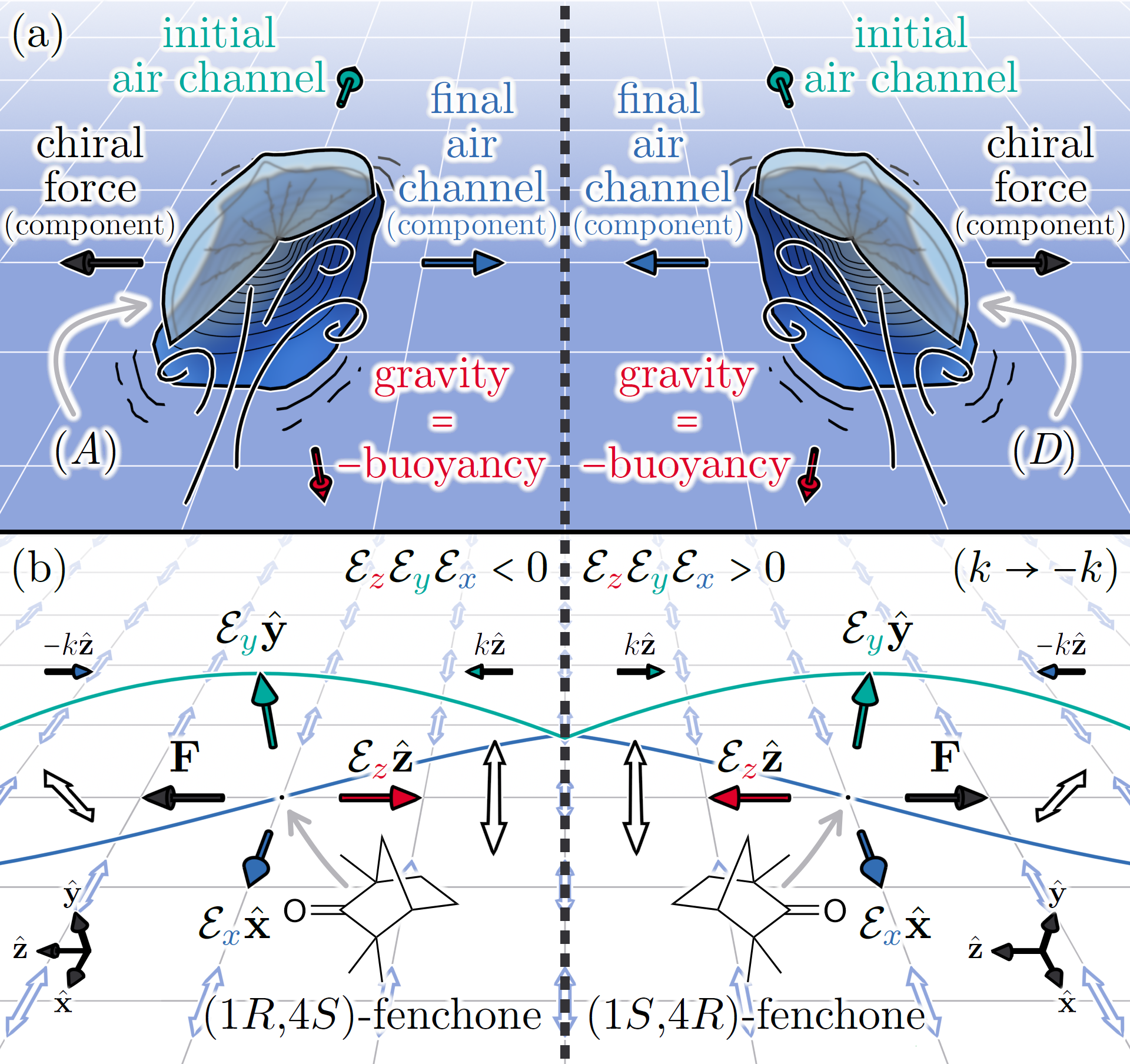
Figure 1: (a) The two distinct mirror-image forms of Velella velella can be separated by the wind. (b) Our chiral optical force $\mathbf{F}$ is constructed by analogy. The double-headed arrows indicate the polarizations of the traveling-wave field $\tilde{\mathbf{E}}^{\prime}$ (blue) and standing-wave field $\tilde{\mathbf{E}}$ (black). Note that the dashed line indicates a complete mirror flip of the molecule and fields, including the standing wave’s wavevectors (three changes in sign for the contributing factors of $\mathbf{F}$). $\mathbf{F}$ also points in opposite directions for opposite enantiomers in a fixed field geometry (one change in sign).

The inspiration for our chiral optical force is Velella velella, the “by-the-wind sailor”; a hydroid colony resembling a small raft with a sail that tilts either antidiagonally (A) or diagonally (D) with respect to a quasi-rectangular base. The two distinct mirror-image forms are sometimes found beached on opposite sides of the Pacific Ocean. It is believed that both are born at sea in roughly equal measure and are then separated by the wind via a force with a chiral component, as illustrated in Fig. 1(a); mother nature potentially uses chirality to minimize the risk of all specimens in a fleet being blown ashore simultaneously Neville76a . The effect can be understood as follows. Gravity together with the buoyancy it gives rise to partially orientate a Vellela velella specimen (pitch and roll) via the specimen’s mass dipole moment. The water further aligns the specimen (yaw) relative to the wind via drag exerted on the specimen’s base. With the specimen’s orientation essentially fixed by gravity and the water, air molecules are transferred from the initial air channel into a final air channel with an orthogonal component via the specimen’s sail. The corresponding momentum transfer gives rise to a force with a chiral component, as claimed. Note that gravity, the initial air channel, and the relevant component of the final air channel form either a left-handed or a right-handed orthogonal triad embodying the chiral sensitivity of the force.

We construct our chiral optical force by analogy, as illustrated in Fig. 1(b). Instead of a Velella velella specimen, we consider a small, polar, diamagnetic, chiral molecule in its vibronic ground state, located at the origin say. Instead of gravity, we consider a strong and homogeneous static electric field

$$\mathbf{E}_{0}={} \mathcal{E}_{z}\hat{\mathbf{z}},$$ (2)

where $\mathcal{E}_{z}$ determines the field’s strength and direction; $\mathbf{E}_{0}$ partially orientates the molecule (pitch and roll) via a dc Stark interaction with the molecule’s permanent electric dipole moment $\boldsymbol{\mu}_{0}$. Instead of the water, we consider an intense and far off-resonance linearly polarized traveling wave with complex electric field

$$\tilde{\mathbf{E}}^{\prime}={} \mathcal{E}_{x}^{\prime}\mathrm{e}^{\mathrm{i}(k^{\prime}y-\omega^{\prime}t)}\hat{\mathbf{x}},$$ (3)

where $\mathcal{E}_{x}^{\prime}$ determines the amplitude and phase of the wave and $\omega^{\prime}$ is the angular frequency, $k^{\prime}=\omega^{\prime}/c$ being the associated angular wavenumber; $\tilde{\mathbf{E}}^{\prime}$ further aligns the molecule (yaw) via an ac Stark interaction with the molecule’s traveling-wave electric dipole-electric dipole polarizability tensor $\alpha(\omega^{\prime})$. Our inclusion here of $\tilde{\mathbf{E}}^{\prime}$ is a vital improvement over our tentative description of $\mathbf{F}$ in Cameron23a , where we assumed quantization along the $x$ axis without explicit justification. Instead of the wind, we consider a relatively weak and far off-resonance lin$\perp$lin standing wave with complex electric field

$$\tilde{\mathbf{E}}={} \mathcal{E}_{y}\mathrm{e}^{\mathrm{i}(kz-\omega t)}\hat{\mathbf{y}}+\mathrm{i}\mathcal{E}_{x}\mathrm{e}^{\mathrm{i}(-kz-\omega t)}\hat{\mathbf{x}},$$ (4)

where $\mathcal{E}_{y}$ determines the amplitude and phase of the $y$ polarized wave, $\mathcal{E}_{x}$ determines the amplitude and phase of the $x$ polarized wave, and $\omega$ is the angular frequency of the waves, $k=\omega/c$ being the associated angular wavenumber; with the molecule’s orientation essentially fixed by $\mathbf{E}_{0}$ and $\tilde{\mathbf{E}}^{\prime}$, photons are transferred from the $y$ polarized wave to the $x$ polarized wave or vice versa via an ac Stark interaction with the molecule’s standing-wave electric dipole-electric dipole polarizability tensor $\alpha(\omega)$ Cohen-Tannoudji11a . The corresponding momentum transfer gives rise to our chiral optical force $\mathbf{F}$. Note that the static field $\mathcal{E}_{z}\hat{\mathbf{z}}$ and the standing-wave polarization vectors $\mathcal{E}_{y}\hat{\mathbf{y}}$ and $\mathcal{E}_{x}\hat{\mathbf{x}}$ form either a left-handed ($\mathcal{E}_{z}\mathcal{E}_{y}\mathcal{E}_{x}<0$) or a right-handed ($\mathcal{E}_{z}\mathcal{E}_{y}\mathcal{E}_{x}>0$) orthogonal triad embodying the chiral sensitivity of $\mathbf{F}$. The analogy with Velella velella is close but there are important differences, in particular the fact that $\mathbf{E}_{0}$ and $\mathbf{F}$ are aligned rather than perpendicular and the fact that the chiralities of the molecule and fields can be chosen independently rather than being immutably correlated.

As our chiral optical force $\mathbf{F}$ is based solely on off-resonance interactions, it does not require a specific energy-level structure and thus has a general applicability not shared by other proposals. The precise values of the angular frequencies $\omega^{\prime}$ and $\omega$ are not critical, however $\omega^{\prime}$ and $\omega$ must differ to help ensure that the principal axes of the molecule’s $\alpha(\omega^{\prime})$ and $\alpha(\omega)$ polarizability ellipsoids are not aligned and thus that $\mathbf{F}$ is non-vanishing in the strong-field limit (see below). For most small molecules, it suffices to choose $\omega^{\prime}$ somewhere in the near infrared and $\omega$ somewhere in the visible, for example.

We take the molecule’s rotational (and nuclear spin) Hamiltonian to have the form

$$H={} V+U+H^{(0)},$$ (5)

where $V$ accounts for the molecule’s interaction with the static field $\mathbf{E}_{0}$ and traveling-wave field $\tilde{\mathbf{E}}^{\prime}$, $U$ accounts for the interaction with the standing-wave field $\tilde{\mathbf{E}}$, and $H^{(0)}$ accounts for the rotational degrees of freedom of the molecule in the absence of the fields. Ideally, we want $V$ to serve as a rotational potential energy and $U$ to serve as a translational potential energy, the field values being chosen such that $U$ does not drastically affect the molecule’s orientation. Neglecting nuclear spin and working to leading order here, we consider

$$V={} -\mathcal{E}_{z}\mu_{0z}-\frac{1}{4}\mathcal{E}_{x}^{\prime 2}\alpha_{xx}(\omega^{\prime}),$$ (6)

$$U={} -\frac{1}{4}\mathcal{E}_{y}^{2}\alpha_{yy}(\omega)-\frac{1}{4}\mathcal{E}_{x}^{2}\alpha_{xx}(\omega)$$

$$-\frac{1}{2}\mathcal{E}_{y}\mathcal{E}_{x}\alpha_{yx}(\omega)\sin(2kZ_{0}),$$ (7)

$$H^{(0)}={} \frac{1}{\hbar^{2}}(CJ^{2}_{c}+BJ^{2}_{b}+AJ^{2}_{a})$$ (8)

with

$$\mu_{0\alpha}={} \ell_{\alpha\alpha^{\prime}}\mu_{0\alpha^{\prime}},$$ (9)

$$\alpha_{\beta\alpha}(\omega^{\prime})={} \ell_{\beta\beta^{\prime}}\ell_{\alpha\alpha^{\prime}}\alpha_{\beta^{\prime}\alpha^{\prime}}(\omega^{\prime}),$$ (10)

$$\alpha_{\beta\alpha}(\omega)={} \ell_{\beta\beta^{\prime}}\ell_{\alpha\alpha^{\prime}}\alpha_{\beta^{\prime}\alpha^{\prime}}(\omega),$$ (11)

where $Z_{0}$ is the lateral position of the molecule; $C<B<A$ are the molecule’s equilibrium rotational constants; $\mathbf{J}$ is the molecule’s rotational angular momentum; $\ell$ is a direction cosine matrix relating the molecule’s principal axes of inertia $c$, $b$, and $a$ to the laboratory axes $z$, $y$, and $x$; and the Einstein summation convention is to be understood with respect to indices $\dots,\beta^{\prime},\alpha^{\prime}\in\{c,b,a\}$ and $\dots,\beta,\alpha\in\{z,y,x\}$ Barron04a ; Bunker05a ; SupplementalMaterial . Let us assume that the molecule’s rotational state has the form

$$|\psi\rangle={} \mathrm{e}^{-\mathrm{i}E_{r}t/\hbar}|r\rangle$$ (12)

with

$$H|r\rangle={} E_{r}|r\rangle,$$ (13)

where $|r\rangle$ is a rotational energy eigenstate and $E_{r}$ is the associated rotational energy eigenvalue. Our chiral optical force then follows as

$$\mathbf{F}={} -\langle\psi|\partial_{Z_{0}}U|\psi\rangle\hat{\mathbf{z}}$$

$$={} k\mathcal{E}_{y}\mathcal{E}_{x}\langle r|\ell_{y\beta^{\prime}}\ell_{x\alpha^{\prime}}|r\rangle\alpha_{\beta^{\prime}\alpha^{\prime}}(\omega)\cos(2kZ_{0})\hat{\mathbf{z}}.$$ (14)

Note that $\mathbf{E}_{0}$ and $\tilde{\mathbf{E}}^{\prime}$ enter into Eq. 14 implicitly via $|r\rangle$.

Our analogy with Velella velella holds in the strong-field regime ($V\gg U,H^{(0)}$), where the static field $\mathbf{E}_{0}$ and traveling-wave field $\tilde{\mathbf{E}}^{\prime}$ significantly hinder the molecule’s rotation. The lowest-lying rotational energy eigenstates $|r\rangle$ are then pendular states in which our chiral optical force tends towards

$$\mathbf{F}\approx{} k\mathcal{E}_{y}\mathcal{E}_{x}\alpha_{yx}(\omega)\rvert_{\Omega}\cos(2kZ_{0})\hat{\mathbf{z}},$$ (15)

where $\Omega$ denotes a molecular orientation for which the rotational potential energy $V$ is minimized. There are two such orientations, as $V$ has two-fold rotational symmetry. A Velella velella specimen’s mass dipole moment, base, and sail constitute a chiral geometry, as illustrated in Fig. 2(a). In general, the molecule’s dipole moment $\boldsymbol{\mu}_{0}$, traveling-wave polarizability $\alpha(\omega^{\prime})$, and standing-wave polarizability $\alpha(\omega)$ constitute an analogous chiral geometry, as illustrated in Fig. 2(b). The sign of the orientated molecule’s dipole moment component $\mu_{0z}\rvert_{\Omega}$ is dictated by the sign of the static field component $\mathcal{E}_{z}$ ($\mathrm{sgn}\,\mu_{0z}\rvert_{\Omega}=\mathrm{sgn}\,\mathcal{E}_{z}$) and the sign of the traveling-wave polarizability component $\alpha_{yx}(\omega)\rvert_{\Omega}$ depends on both the sign of $\mu_{0z}\rvert_{\Omega}$ and the molecule’s chirality. According to Eq. 15, the direction of $\mathbf{F}$ thus depends (implicitly) on the molecule’s chirality via the sign of the product $[\mu_{0z}\alpha_{yx}(\omega)]\rvert_{\Omega}$ and on the field’s chirality via the sign of the product $\mathcal{E}_{z}\mathcal{E}_{y}\mathcal{E}_{x}$. Note that with the molecule’s orientation essentially fixed by $\mathbf{E}_{0}$ and $\tilde{\mathbf{E}}^{\prime}$ via $V$, the translational potential energy $U\rvert_{\Omega}$ is minimized when the polarization of the standing-wave field $\tilde{\mathbf{E}}$ is linear and quasi-parallel to the short axis of the projection of the $\alpha(\omega)$ polarizability ellipsoid in the $y$-$x$ plane. For $\alpha_{yx}(\omega)\rvert_{\Omega}\lessgtr 0$, this occurs when $\sin(2kZ_{0})=\mp 1$; $\mathbf{F}$ pushes the molecule towards the nearest local minimum in $U\rvert_{\Omega}$.

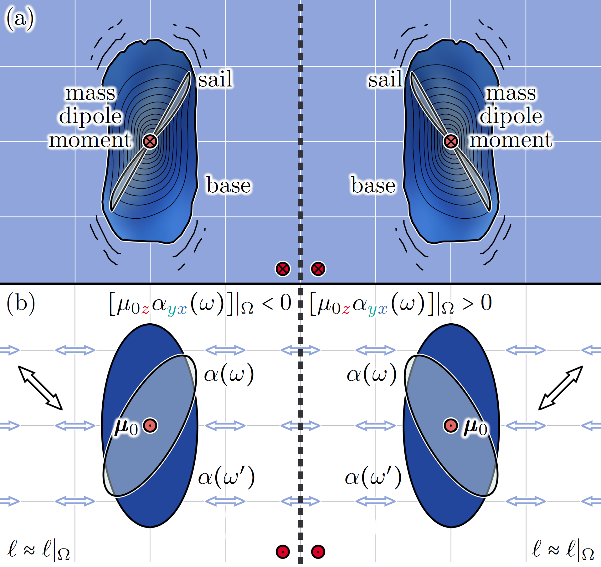
Figure 2: (a) The key elements of a Velella velella specimen. (b) The analogous molecular properties with the molecule’s orientation assumed close to a minimum of the rotational potential energy $V$. The double-headed black arrows here indicate the orthogonal linear polarizations of the standing-wave field $\tilde{\mathbf{E}}$ where the translational potential energy $U\rvert_{\Omega}$ is minimized.

Also of interest for some molecules (see below) is the weak-field regime ($U\ll V\ll H^{(0)}$), where the static field $\mathbf{E}_{0}$ and traveling-wave field $\tilde{\mathbf{E}}^{\prime}$ only slightly affect the rotation of the molecule. A perturbative treatment of the rotational energy eigenstate $|r\rangle$ valid to first order in the rotational potential energy $V$ with the translational potential energy $U$ neglected reveals that our chiral optical force tends towards the form

$$\mathbf{F}\approx{} k\mathcal{E}_{z}\mathcal{E}_{y}\mathcal{E}_{x}[\mathcal{C}_{r}\mu_{0c}\alpha_{ba}(\omega)+\mathcal{B}_{r}\mu_{0b}\alpha_{ac}(\omega)+\mathcal{A}_{r}\mu_{0a}\alpha_{cb}(\omega)]$$

$$\times\cos(2kZ_{0})\hat{\mathbf{z}},$$ (16)

where $\mathcal{C}_{r}$, $\mathcal{B}_{r}$, and $\mathcal{A}_{r}$ are chirally insensitive coefficients, the values of which depend on the molecule’s rotational state Cameron23a ; SupplementalMaterial . According to Eq. 16, the direction of $\mathbf{F}$ depends on the molecule’s chirality via the products $\mu_{0c}\alpha_{ba}(\omega)$, $\mu_{0b}\alpha_{ac}(\omega)$, and $\mu_{0a}\alpha_{cb}(\omega)$ and on the field’s chirality via the product $\mathcal{E}_{z}\mathcal{E}_{y}\mathcal{E}_{x}$.

Between the extremes of the strong-field limit given by Eq. 15 and the weak-field limit given by Eq. 16, our chiral optical force $\mathbf{F}$ has to be calculated using Eq. 14 with the rotational energy eigenstate $|r\rangle$ obtained numerically. In general, we find that the associated rotational energy eigenvalue and required expectation value have the forms

$$E_{r}=-\Delta_{r}-\frac{1}{2}\mathcal{E}_{y}\mathcal{E}_{x}\chi_{r}\sin(2kZ_{0})$$

$$-\mathcal{E}_{y}\mathcal{E}_{x}\sum_{n=1}^{\infty}\frac{1}{2(n+1)}\Upsilon_{r}^{(n)}\sin^{n+1}(2kZ_{0}),$$ (17)

$$\langle r|\ell_{y\beta^{\prime}}\ell_{x\alpha^{\prime}}|r\rangle\alpha_{\beta^{\prime}\alpha^{\prime}}(\omega)=\chi_{r}+\sum_{n=1}^{\infty}\Upsilon_{r}^{(n)}\sin^{n}(2kZ_{0}),$$ (18)

where $\Delta_{r}$ is an energy offset, $\chi_{r}$ is the leading effective polarizability, and the $\Upsilon_{r}^{(n)}$ embody corrections due to the unwanted effect of the translational potential energy $U$ on the molecule’s orientation. Symmetry arguments dictate that $\Delta_{r}$ and the odd $\Upsilon_{r}^{(n)}$ are chirally insensitive whereas $\chi_{r}$ and the even $\Upsilon_{r}^{(n)}$ have opposite signs for opposite enantiomers. The values of $\Delta_{r}$, $\chi_{r}$, and the $\Upsilon_{r}^{(n)}$ depend on the molecule’s rotational state. Note that the $\Upsilon_{r}^{(n)}$ contribute nothing to $\mathbf{F}$ when $\sin(2kZ_{0})=0$ and that Eqs. 17 and 18 are consistent with the requirement that $\mathbf{F}=-\partial_{Z_{0}}E_{r}\hat{\mathbf{z}}$.

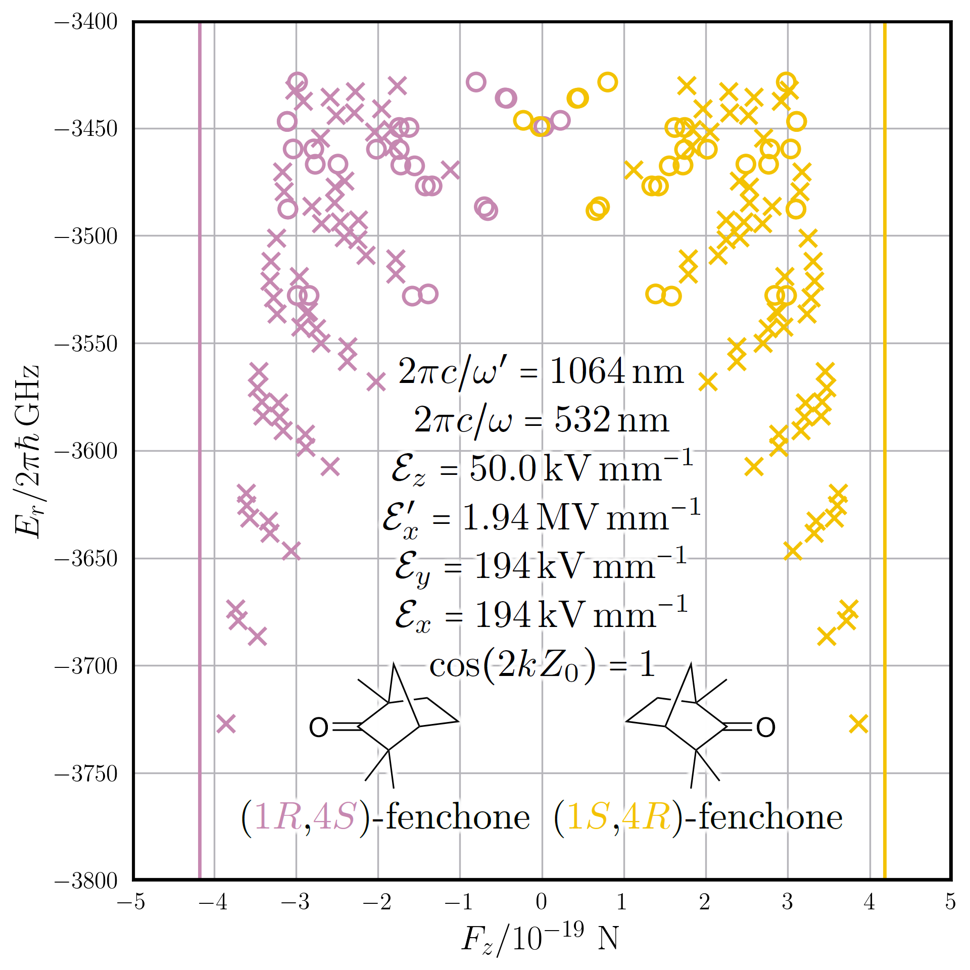
Figure 3: A scatter plot of our chiral optical force $F_{z}$ versus rotational energy eigenvalue $E_{r}$ for the first $150$ rotational states of the opposite enantiomers of fenchone. Crosses are two-fold quasi-degenerate ($5\%$ tolerance) and circles are non-degenerate. Vertical lines indicate the strong-field limits given by Eq. 15. We have chosen $2\omega^{\prime}=\omega$ simply to facilitate experimental realization using a single light source. Note that the field has a fixed right-handed geometry ($\mathcal{E}_{z}\mathcal{E}_{y}\mathcal{E}_{x}>0$) with intensities of $I^{\prime}=\epsilon_{0}c\mathcal{E}_{x}^{\prime 2}/2=5.00\times 10^{11}\,\mathrm{W}\,\mathrm{cm}^{-2}$ and $I=\epsilon_{0}c(\mathcal{E}_{y}^{2}+\mathcal{E}_{x}^{2})/2=1.00\times 10^{10}\,\mathrm{W}\,\mathrm{cm}^{-2}$.

Shown in Fig. 3 are results calculated for the opposite enantiomers of fenchone SupplementalMaterial . The (1R,4S) enantiomer can be found in wormwood, tansy and cedarleaf whereas the (1S,4R) enantiomer can be found in wild, bitter and sweet fennel Ravid92a ; both can be present in absinthe, “the green fairy” Nathan-Maister09a . The states of lowest energy are close to the strong-field limits of $F_{z}=\mp 4.18^{-19}\,\mathrm{N}$ given by Eq. 15. In contrast, Eq. 1 gives $|\mathbf{F}^{\prime}|\leq 7\times 10^{-22}\,\mathrm{N}$ for the enantiomers of fenchone in a one-dimensional optical helicity lattice with commensurate parameters Cameron14b ; Cameron14c ; our chiral optical force $\mathbf{F}$ is nearly three orders of magnitude stronger here than the corresponding optical helicity gradient force $\mathbf{F}^{\prime}$. As the energy increases, the strong-field criterion $V\gg H^{(0)}$ begins to break down and the force values deviate accordingly. The overall enantioselectivity is excellent in the range shown; for each enantiomer, $F_{z}$ has the same sign for $148$ of the $150$ rotational states considered. It continues to degrade as the rotational energy is increased (not shown). Note that the plots for the opposite enantiomers are mirror images of each other, as they should be.

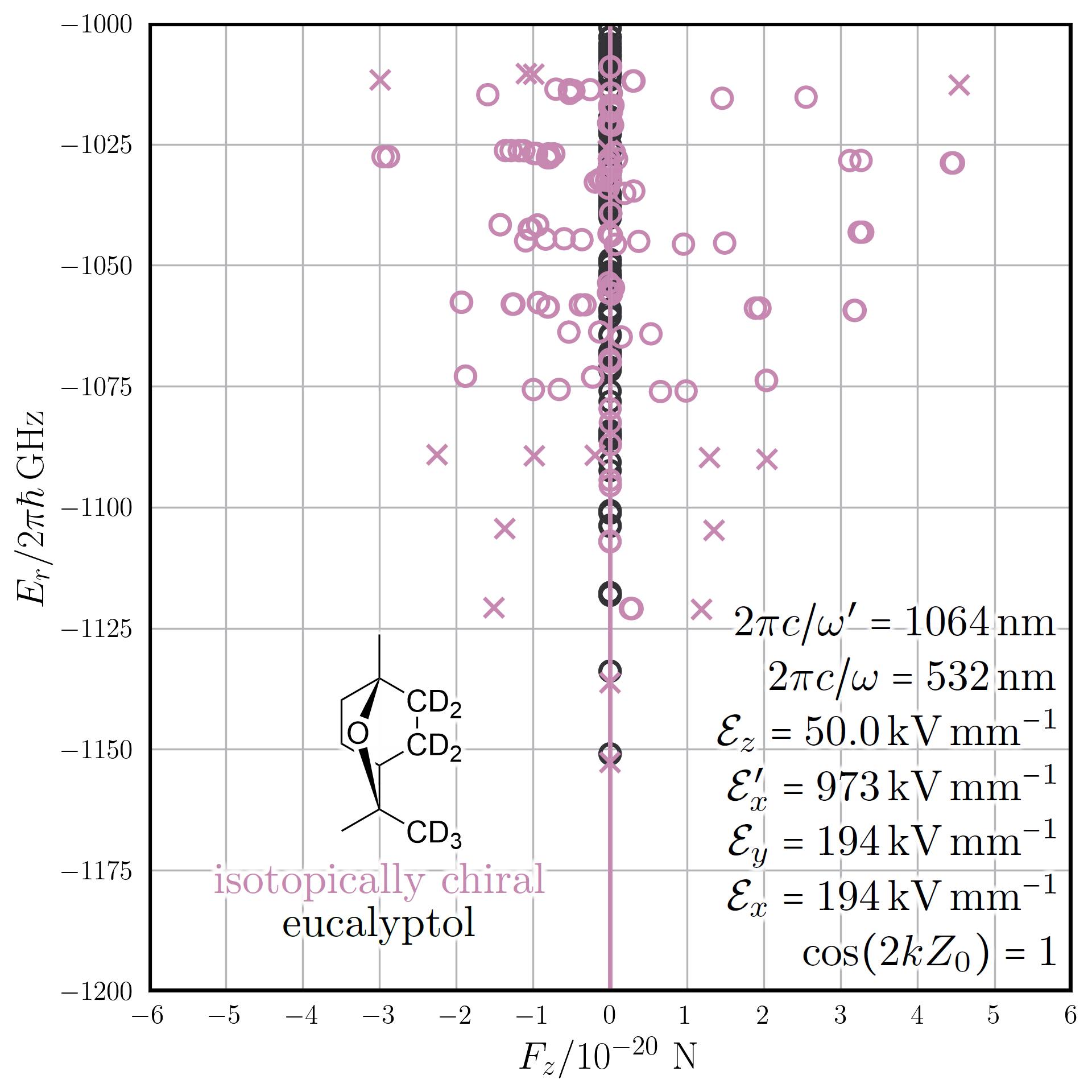
Figure 4: As in Fig. 3 but for a single enantiomer of isotopically chiral eucalyptol and an optimized intensity of $I^{\prime}=\epsilon_{0}c\mathcal{E}_{x}^{\prime 2}/2=1.26\times 10^{11}\,\mathrm{W}\,\mathrm{cm}^{-2}$. Results for achiral eucalyptol ($F_{z}=0$) are shown in dark grey for comparison.

Isotopically chiral molecules constitute an interesting and potentially very important special case for our chiral optical force $\mathbf{F}$. The opposite enantiomers of an isotopically chiral molecule differ solely by the arrangement of their neutrons, making them notoriously difficult to separate using existing methods Kimata97a . As the electronic properties of an isotopically chiral molecule are achiral to leading order, the dipole moment $\boldsymbol{\mu}_{0}$, traveling-wave polarizability $\alpha(\omega^{\prime})$, and standing-wave polarizability $\alpha(\omega)$ do not constitute a significantly chiral geometry and the strong-field limit given by Eq. 15 is essentially zero (neglecting vibrational contributions). The mass distribution is chiral, however, and affects the principal axes of inertia $c$, $b$, and $a$ such that one or more of the products $\mu_{0c}\alpha_{ba}(\omega)$, $\mu_{0b}\alpha_{ac}(\omega)$, and $\mu_{0a}\alpha_{cb}(\omega)$ is usually non-zero and the weak-field limit given by Eq. 16 yields non-trivial results, similar to an ordinary chiral molecule. Optima can be found between these extremes. Shown in Fig. 4 are results calculated for an enantiomer of isotopically chiral eucalyptol SupplementalMaterial . The states of lowest energy approach the strong-field limit of $F_{z}=0$ given by Eq. 15. As the energy increases, the molecule’s chiral mass distribution comes into play via the unperturbed rotational Hamiltonian $H^{(0)}$ and the force values reach sizeable magnitudes of $|\mathbf{F}|\sim 10^{-20}\,\mathrm{N}$. In contrast, Eq. 1 gives $\mathbf{F}^{\prime}\approx 0$ for isotopically chiral molecules, as $G^{\prime}(\omega)\approx 0$. The overall enantioselectivity is poor; for the enantiomer under consideration, $F_{z}<0$ for $87/150$ of the rotational states shown. Let us emphasize, however, that for each rotational state individually, the enantioselectivity is perfect; $F_{z}$ points in the opposite direction for the opposite enantiomer (not depicted).

Shown in Fig. 5(a) is our proposed experiment. The key elements can be summarized as follows. A beam of molecules emerges from a buffer gas source, internally cooled to temperature $T$ Hutzler12a . Skimmers collimate and velocity select the beam, giving initial molecular wavepackets of width $\sigma$ and linear momentum $\hbar K\hat{\mathbf{x}}$, where $K$ is the angular wavenumber. A mechanical grating transmits only those molecules for which $\cos(2kZ_{0})\geq 0$ into the interaction region, where electrodes produce the static field $\mathbf{E}_{0}$ whilst a pulsed laser source produces the traveling-wave field $\tilde{\mathbf{E}}^{\prime}$ and the standing-wave field $\mathbf{E}$ to exert our chiral optical force $\mathbf{F}$ for a time $\tau$. The molecules then propagate freely through a distance $L$ to a detection screen, where opposite enantiomers are found to be spatially separated. Shown in Fig. 5(b) are deflection patterns calculated for the enantiomers of fenchone SupplementalMaterial . A significant separation is apparent.

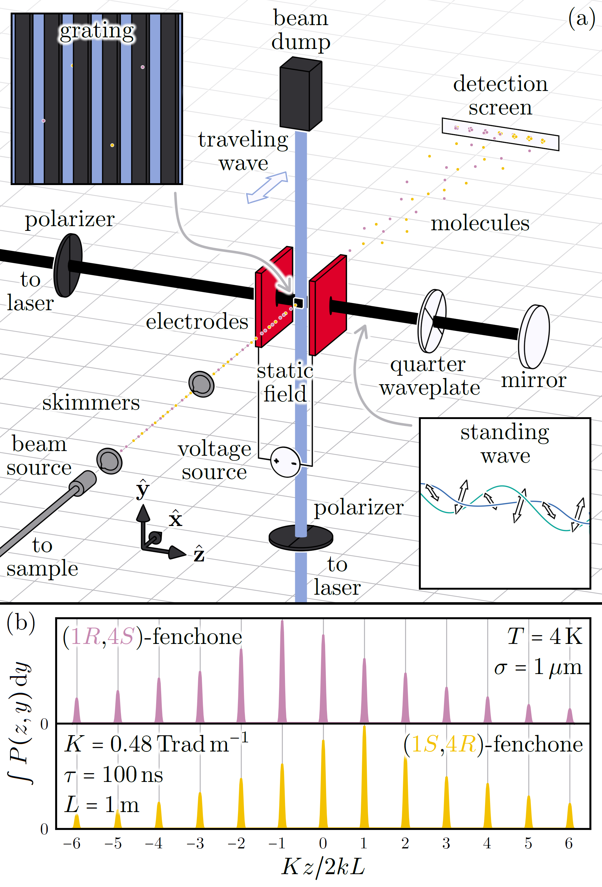
Figure 5: (a) A proposed experiment to separate the opposite enantiomers of a chiral molecule using our chiral optical force $\mathbf{F}$. (b) A molecular deflection pattern, calculated using the parameters shown in Fig. 3 and here. Note that the separation between orders is $2kL/K=49\,\mu\mathrm{m}$.

Our work can be regarded as part of the ongoing “electric dipole revolution in chiral measurements” Ayuso22a . Of particular interest are recent proposals for enantiosensitive light bending Ayuso21a and steering of free induction decay Khokhlova22a ; the use of chiral molecules to deflect photons. Our proposal is complementary; the use of photons to deflect chiral molecules.

Inspired by nature, we have identified a robust chiral optical force for chiral molecules that arises via electric dipole interactions alone, the key ingredient being suitable molecular orientation. We conclude by noting that instead of the static and traveling-wave fields considered explicitly in this Letter, the required molecular orientation might be realized using surfaces, potentially opening the door to separation schemes with high throughput.

R.P.C. and D.M. gratefully acknowledge the support of the Royal Society (URF$\backslash$R1$\backslash$191243, RF$\backslash$ERE$\backslash$210170, RF$\backslash$ERE$\backslash$231130, and URF$\backslash$R$\backslash$241008). R.P.C. is a Royal Society University Research Fellow. N.V. and D.W. acknowledge the Deutsche Forschungsgemeinschaft for support (project 328961117) through the Collaborative Research Center ELCH (SFB 1319).

Appendix A Asymmetric rigid rotor

The quantum-mechanical description of the asymmetric rigid rotor has been covered extensively elsewhere. We use the conventions below, which are slightly unusual in that we consider quantization along the $x$ axis rather than the $z$ axis.

We take the molecule’s principal axes of inertia $c$, $b$, and $a$ to be associated with direction cosines given by

$$\ell_{zc}={} -\cos\theta\sin\phi\sin\chi+\cos\phi\cos\chi,$$ (19)

$$\ell_{zb}={} \cos\theta\sin\phi\cos\chi+\cos\phi\sin\chi,$$ (20)

$$\ell_{za}={} \sin\theta\sin\phi,$$ (21)

$$\ell_{yc}={} -\cos\theta\cos\phi\sin\chi-\sin\phi\cos\chi,$$ (22)

$$\ell_{yb}={} \cos\theta\cos\phi\cos\chi-\sin\phi\sin\chi,$$ (23)

$$\ell_{ya}={} \sin\theta\cos\phi,$$ (24)

$$\ell_{xc}={} \sin\theta\sin\chi,$$ (25)

$$\ell_{xb}={} -\sin\theta\cos\chi,$$ (26)

$$\ell_{xa}={} \cos\theta,$$ (27)

where $0\leq\theta\leq\pi$, $0\leq\phi<2\pi$, and $0\leq\chi<2\pi$ are Euler angles relating $c$, $b$, and $a$ to the laboratory axes $z$, $y$, and $x$. The molecule-fixed components of the molecule’s rotational angular momentum $\mathbf{J}$ are

$$J_{c}={} -\mathrm{i}\hbar\left(\cos\chi\frac{\partial}{\partial\theta}+\csc\theta\sin\chi\frac{\partial}{\partial\phi}-\cot\theta\sin\chi\frac{\partial}{\partial\chi}\right),$$ (28)

$$J_{b}={} -\mathrm{i}\hbar\left(\sin\chi\frac{\partial}{\partial\theta}-\csc\theta\cos\chi\frac{\partial}{\partial\phi}+\cot\theta\cos\chi\frac{\partial}{\partial\chi}\right),$$ (29)

$$J_{a}={} -\mathrm{i}\hbar\frac{\partial}{\partial\chi}.$$ (30)

The laboratory-fixed components of $\mathbf{J}$ are

$$J_{z}={} -\mathrm{i}\hbar\left(\cos\phi\frac{\partial}{\partial\theta}-\cot\theta\sin\phi\frac{\partial}{\partial\phi}+\csc\theta\sin\phi\frac{\partial}{\partial\chi}\right),$$ (31)

$$J_{y}={} -\mathrm{i}\hbar\left(-\sin\phi\frac{\partial}{\partial\theta}-\cot\theta\cos\phi\frac{\partial}{\partial\phi}+\csc\theta\cos\phi\frac{\partial}{\partial\chi}\right),$$ (32)

$$J_{x}={} -\mathrm{i}\hbar\frac{\partial}{\partial\phi}.$$ (33)

We take the unperturbed rotational energy eigenstates $|J_{\tau},m\rangle^{(0)}$ and associated energy eigenvalues $E_{J_{\tau}}^{(0)}$ to satisfy

$$H^{(0)}|J_{\tau},m\rangle^{(0)}={} E_{J_{\tau}}^{(0)}|J_{\tau},m\rangle^{(0)},$$ (34)

$$(J_{c}^{2}+J_{b}^{2}+J_{a}^{2})|J_{\tau},m\rangle^{(0)}={} J(J+1)\hbar^{2}|J_{\tau},m\rangle^{(0)},$$ (35)

$$J_{x}|J_{\tau},m\rangle^{(0)}={} m\hbar|J_{\tau},m\rangle^{(0)},$$ (36)

where $J\in\{0,1,\dots\}$ is the rotational angular momentum quantum number, $\tau\in\{-J,\dots,J\}$ is a label that increases with increasing energy, and $m\in\{-J,\dots,J\}$ is the laboratory-fixed rotational angular momentum projection quantum number.

To help us identify the unperturbed rotational energy eigenstates $|J_{\tau},m\rangle^{(0)}$ and associated energy eigenvalues $E_{J_{\tau}}^{(0)}$ explicitly, we work in a basis of unperturbed symmetric rigid rotor states $|J,\kappa,m\rangle^{(0)}$ satisfying

$$(J_{c}^{2}+J_{b}^{2}+J_{a}^{2})|J,\kappa,m\rangle^{(0)}={} J(J+1)\hbar^{2}|J,\kappa,m\rangle^{(0)},$$ (37)

$$J_{a}|J,\kappa,m\rangle^{(0)}={} \kappa\hbar|J,\kappa,m\rangle^{(0)},$$ (38)

$$J_{x}|J,\kappa,m\rangle^{(0)}={} m\hbar|J,\kappa,m\rangle^{(0)},$$ (39)

where $\kappa\in\{-J,\dots,J\}$ is the molecule-fixed rotational angular momentum projection quantum number, the corresponding wavefunctions $\langle\theta,\phi,\chi|J,\kappa,m\rangle^{(0)}$ being given by

$$\langle\theta,\phi,\chi|J,\kappa,m\rangle^{(0)}={} \sqrt{\frac{(J+m)!(J-m)!(J+\kappa)!(J-\kappa)!(2J+1)}{8\pi^{2}}}\mathrm{e}^{\mathrm{i}m\phi}\mathrm{e}^{\mathrm{i}\kappa\chi}$$

$$\times\sum_{\sigma=\mathrm{max}(0,\kappa-m)}^{\mathrm{min}(J-m,J+\kappa)}(-1)^{\sigma}\frac{[\cos(\theta/2)]^{2J+\kappa-m-2\sigma}[-\sin(\theta/2)]^{m-\kappa+2\sigma}}{\sigma!(J-m-\sigma)!(m-\kappa+\sigma)!(J+\kappa-\sigma)!}.$$ (40)

The $|J,\kappa,m\rangle^{(0)}$ render the unperturbed rotational Hamiltonian $H^{(0)}$ block diagonal in the quantum number $J$, as

$${}^{(0)}\langle J^{\prime},\kappa^{\prime},m^{\prime}|H^{(0)}|J,\kappa,m\rangle^{(0)}={} \frac{1}{2}J(J+1)(C+B)\delta_{J^{\prime}J}\delta_{\kappa^{\prime}\kappa}\delta_{m^{\prime}m}-\kappa^{2}\left[\frac{1}{2}(C+B)-A\right]\delta_{J^{\prime}J}\delta_{\kappa^{\prime}\kappa}\delta_{m^{\prime}m}$$

$$-\frac{1}{4}\sqrt{[J(J+1)-\kappa(\kappa-1)][J(J+1)-(\kappa-1)(\kappa-2)]}(C-B)\delta_{J^{\prime}J}\delta_{\kappa^{\prime}\kappa-2}\delta_{m^{\prime}m}$$

$$-\frac{1}{4}\sqrt{[J(J+1)-\kappa(\kappa+1)][J(J+1)-(\kappa+1)(\kappa+2)]}(C-B)\delta_{J^{\prime}J}\delta_{\kappa^{\prime}\kappa+2}\delta_{m^{\prime}m}.$$ (41)

The diagonalization of $H^{(0)}$ can completed analytically for $J\in\{0,\dots,5\}$, giving

$$|0_{0},0\rangle^{(0)}={} |0,0,0\rangle^{(0)},$$ (42)

$$|1_{-1},m\rangle^{(0)}={} |1,0,m\rangle^{(0)},$$ (43)

$$|1_{0},m\rangle^{(0)}={} \frac{1}{\sqrt{2}}(|1,1,m\rangle^{(0)}-|1,-1,m\rangle^{(0)}),$$ (44)

$$|1_{1},m\rangle^{(0)}={} \frac{1}{\sqrt{2}}(|1,1,m\rangle^{(0)}+|1,-1,m\rangle^{(0)})$$ (45)

with

$$E_{0_{0}}^{(0)}={} 0,$$ (46)

$$E_{1_{-1}}^{(0)}={} C+B,$$ (47)

$$E_{1_{0}}^{(0)}={} C+A,$$ (48)

$$E_{1_{1}}^{(0)}={} B+A,$$ (49)

for example. The diagonalization of $H^{(0)}$ must be completed numerically for $J\in\{6,\dots\}$.

In the symmetric rotor basis, we have

$${}^{(0)}\langle J^{\prime},\kappa^{\prime},m^{\prime}|\ell_{zc}|J,\kappa,m\rangle^{(0)}={} F_{J^{\prime}J}G_{J^{\prime}\kappa^{\prime}J\kappa}H_{J^{\prime}m^{\prime}Jm}(-\mathrm{i}\delta_{\kappa^{\prime}\kappa-1}+\mathrm{i}\delta_{\kappa^{\prime}\kappa+1})(\mathrm{i}\delta_{m^{\prime}m-1}-\mathrm{i}\delta_{m^{\prime}m+1}),$$ (50)

$${}^{(0)}\langle J^{\prime},\kappa^{\prime},m^{\prime}|\ell_{zb}|J,\kappa,m\rangle^{(0)}={} F_{J^{\prime}J}G_{J^{\prime}\kappa^{\prime}J\kappa}H_{J^{\prime}m^{\prime}Jm}(\delta_{\kappa^{\prime}\kappa-1}+\delta_{\kappa^{\prime}\kappa+1})(\mathrm{i}\delta_{m^{\prime}m-1}-\mathrm{i}\delta_{m^{\prime}m+1}),$$ (51)

$${}^{(0)}\langle J^{\prime},\kappa^{\prime},m^{\prime}|\ell_{za}|J,\kappa,m\rangle^{(0)}={} F_{J^{\prime}J}G_{J^{\prime}\kappa^{\prime}J\kappa}H_{J^{\prime}m^{\prime}Jm}\delta_{\kappa^{\prime}\kappa}(\mathrm{i}\delta_{m^{\prime}m-1}-\mathrm{i}\delta_{m^{\prime}m+1}),$$ (52)

$${}^{(0)}\langle J^{\prime},\kappa^{\prime},m^{\prime}|\ell_{yc}|J,\kappa,m\rangle^{(0)}={} F_{J^{\prime}J}G_{J^{\prime}\kappa^{\prime}J\kappa}H_{J^{\prime}m^{\prime}Jm}(-\mathrm{i}\delta_{\kappa^{\prime}\kappa-1}+\mathrm{i}\delta_{\kappa^{\prime}\kappa+1})(\delta_{m^{\prime}m-1}+\delta_{m^{\prime}m+1}),$$ (53)

$${}^{(0)}\langle J^{\prime},\kappa^{\prime},m^{\prime}|\ell_{yb}|J,\kappa,m\rangle^{(0)}={} F_{J^{\prime}J}G_{J^{\prime}\kappa^{\prime}J\kappa}H_{J^{\prime}m^{\prime}Jm}(\delta_{\kappa^{\prime}\kappa-1}+\delta_{\kappa^{\prime}\kappa+1})(\delta_{m^{\prime}m-1}+\delta_{m^{\prime}m+1}),$$ (54)

$${}^{(0)}\langle J^{\prime},\kappa^{\prime},m^{\prime}|\ell_{ya}|J,\kappa,m\rangle^{(0)}={} F_{J^{\prime}J}G_{J^{\prime}\kappa^{\prime}J\kappa}H_{J^{\prime}m^{\prime}Jm}\delta_{\kappa^{\prime}\kappa}(\delta_{m^{\prime}m-1}+\delta_{m^{\prime}m+1}),$$ (55)

$${}^{(0)}\langle J^{\prime},\kappa^{\prime},m^{\prime}|\ell_{xc}|J,\kappa,m\rangle^{(0)}={} F_{J^{\prime}J}G_{J^{\prime}\kappa^{\prime}J\kappa}H_{J^{\prime}m^{\prime}Jm}(-\mathrm{i}\delta_{\kappa^{\prime}\kappa-1}+\mathrm{i}\delta_{\kappa^{\prime}\kappa+1})\delta_{m^{\prime}m},$$ (56)

$${}^{(0)}\langle J^{\prime},\kappa^{\prime},m^{\prime}|\ell_{xb}|J,\kappa,m\rangle^{(0)}={} F_{J^{\prime}J}G_{J^{\prime}\kappa^{\prime}J\kappa}H_{J^{\prime}m^{\prime}Jm}(\delta_{\kappa^{\prime}\kappa-1}+\delta_{\kappa^{\prime}\kappa+1})\delta_{m^{\prime}m},$$ (57)

$${}^{(0)}\langle J^{\prime},\kappa^{\prime},m^{\prime}|\ell_{xa}|J,\kappa,m\rangle^{(0)}={} F_{J^{\prime}J}G_{J^{\prime}\kappa^{\prime}J\kappa}H_{J^{\prime}m^{\prime}Jm}\delta_{\kappa^{\prime}\kappa}\delta_{m^{\prime}m}$$ (58)

with

$$F_{J^{\prime}J}={} \frac{1}{4(J+\delta_{0J})\sqrt{(2J-1)(2J+1)}}\delta_{J^{\prime}J-1}+\frac{1}{4(J+\delta_{0J})(J+1)}\delta_{J^{\prime}J}+\frac{1}{4(J+1)\sqrt{4(J+1)^{2}-1}}\delta_{J^{\prime}J+1},$$ (59)

$$G_{J^{\prime}\kappa^{\prime}J\kappa}={} -\sqrt{(J+\kappa-1)(J+\kappa)}\delta_{J^{\prime}J-1}\delta_{\kappa^{\prime}\kappa-1}+\sqrt{(J-\kappa+1)(J+\kappa)}\delta_{J^{\prime}J}\delta_{\kappa^{\prime}\kappa-1}+\sqrt{(J-\kappa+2)(J-\kappa+1)}\delta_{J^{\prime}J+1}\delta_{\kappa^{\prime}\kappa-1}$$

$$+2\sqrt{J^{2}-\kappa^{2}}\delta_{J^{\prime}J-1}\delta_{\kappa^{\prime}\kappa}+2\kappa\delta_{J^{\prime}J}\delta_{\kappa^{\prime}\kappa}+2\sqrt{(J+1)^{2}-\kappa^{2}}\delta_{J^{\prime}J+1}\delta_{\kappa^{\prime}\kappa}+\sqrt{(J-\kappa-1)(J-\kappa)}\delta_{J^{\prime}J-1}\delta_{\kappa^{\prime}\kappa+1}$$

$$+\sqrt{(J+\kappa+1)(J-\kappa)}\delta_{J^{\prime}J}\delta_{\kappa^{\prime}\kappa+1}-\sqrt{(J+\kappa+2)(J+\kappa+1)}\delta_{J^{\prime}J+1}\delta_{\kappa^{\prime}\kappa+1},$$ (60)

$$H_{J^{\prime}m^{\prime}Jm}={} -\sqrt{(J+m-1)(J+m)}\delta_{J^{\prime}J-1}\delta_{m^{\prime}m-1}+\sqrt{(J-m+1)(J+m)}\delta_{J^{\prime}J}\delta_{m^{\prime}m-1}$$

$$+\sqrt{(J-m+2)(J-m+1)}\delta_{J^{\prime}J+1}\delta_{m^{\prime}m-1}+2\sqrt{J^{2}-m^{2}}\delta_{J^{\prime}J-1}\delta_{m^{\prime}m}+2m\delta_{J^{\prime}J}\delta_{m^{\prime}m}$$

$$+2\sqrt{(J+1)^{2}-m^{2}}\delta_{J^{\prime}J+1}\delta_{m^{\prime}m}+\sqrt{(J-m-1)(J-m)}\delta_{J^{\prime}J-1}\delta_{m^{\prime}m+1}+\sqrt{(J+m+1)(J-m)}\delta_{J^{\prime}J}\delta_{m^{\prime}m+1}$$

$$-\sqrt{(J+m+2)(J+m+1)}\delta_{J^{\prime}J+1}\delta_{m^{\prime}m+1},$$ (61)

where $F_{J^{\prime}J}$, $G_{J^{\prime}\kappa^{\prime}J\kappa}$, and $H_{J^{\prime}m^{\prime}Jm}$ are useful shorthands.

Appendix B $\mathcal{C}_{r}$, $\mathcal{B}_{r}$, and $\mathcal{A}_{r}$

Basic perturbation theory valid to first order in the rotational potential energy $V$ with the translational potential energy $U$ neglected gives

$$|J_{\tau},m\rangle\approx{} |J_{\tau},m\rangle^{(0)}+|J_{\tau},m\rangle^{(1)}$$ (62)

with

$$|J_{\tau},m\rangle^{(1)}={} \sum_{\begin{subarray}{c}J^{\prime},\tau^{\prime},m^{\prime}\\ \neq J,\tau,m\end{subarray}}\frac{{}^{(0)}\langle J^{\prime}_{\tau^{\prime}},m^{\prime}|V|J_{\tau},m\rangle^{(0)}}{E_{J_{\tau}}^{(0)}-E_{J^{\prime}_{\tau^{\prime}}}^{(0)}}|J^{\prime}_{\tau^{\prime}},m^{\prime}\rangle^{(0)},$$ (63)

where $|J_{\tau},m\rangle^{(1)}$ is the first-order correction to the unperturbed rotational energy eigenstate $|J_{\tau},m\rangle^{(0)}$. Note that ${}^{(0)}\langle J_{\tau},m^{\prime}|V|J_{\tau},m\rangle^{(0)}\propto\delta_{m^{\prime}m}$ is diagonal in the quantum number $m$, as is required for the self-consistent application of the perturbation theory; the asymmetric rigid rotor has no linear dc Stark shift and the $|J_{\tau},m\rangle^{(0)}$ are quantized along $x$, matching the polarization axis of the traveling-wave field $\tilde{\mathbf{E}}^{\prime}$. To first order in $V$, the expectation value required to evaluate our chiral optical force $\mathbf{F}$ is

$$\langle{} J_{\tau},m|\ell_{y\beta^{\prime}}\ell_{x\alpha^{\prime}}|J_{\tau},m\rangle\alpha_{\beta^{\prime}\alpha^{\prime}}(\omega)\approx{}^{(0)}\langle J_{\tau},m|\ell_{y\beta^{\prime}}\ell_{x\alpha^{\prime}}|J_{\tau},m\rangle^{(0)}\alpha_{\beta^{\prime}\alpha^{\prime}}(\omega)$$

$$+\sum_{\begin{subarray}{c}J^{\prime},\tau^{\prime},m^{\prime}\\ \neq J,\tau,m\end{subarray}}\frac{2\mathcal{E}_{z}}{E_{J^{\prime}_{\tau^{\prime}}}^{(0)}-E_{J_{\tau}}^{(0)}}\Re({}^{(0)}\langle J_{\tau},m|\ell_{z\gamma^{\prime}}|J^{\prime}_{\tau^{\prime}},m^{\prime}\rangle^{(0)}{}^{(0)}\langle J^{\prime}_{\tau^{\prime}},m^{\prime}|\ell_{y\beta^{\prime}}\ell_{x\alpha^{\prime}}|J_{\tau},m\rangle^{(0)})\mu_{0\gamma^{\prime}}\alpha_{\beta^{\prime}\alpha^{\prime}}(\omega)$$

$$+\sum_{\begin{subarray}{c}J^{\prime},\tau^{\prime},m^{\prime}\\ \neq J,\tau,m\end{subarray}}\frac{\mathcal{E}_{x}^{\prime 2}}{2(E_{J^{\prime}_{\tau^{\prime}}}^{(0)}-E_{J_{\tau}}^{(0)})}\Re({}^{(0)}\langle J_{\tau},m|\ell_{x\delta^{\prime}}\ell_{x\gamma^{\prime}}|J^{\prime}_{\tau^{\prime}},m^{\prime}\rangle^{(0)}{}^{(0)}\langle J^{\prime}_{\tau^{\prime}},m^{\prime}|\ell_{y\beta^{\prime}}\ell_{x\alpha^{\prime}}|J_{\tau},m\rangle^{(0)})\alpha_{\delta^{\prime}\gamma^{\prime}}(\omega^{\prime})\alpha_{\beta^{\prime}\alpha^{\prime}}(\omega).$$ (64)

Explicit calculation reveals that the first and final terms in Eq. 64 vanish. As $\mu_{0c}\alpha_{ba}(\omega)=\mu_{0c}\alpha_{ab}(\omega)$, $\mu_{0b}\alpha_{ac}(\omega)=\mu_{0b}\alpha_{ca}(\omega)$, and $\mu_{0a}\alpha_{cb}(\omega)=\mu_{0a}\alpha_{bc}(\omega)$ are the only components of the product $\mu_{0\gamma^{\prime}}\alpha_{\beta^{\prime}\alpha^{\prime}}(\omega)$ that are uniquely signed and thus directly observable for the asymmetric rigid rotor, this leaves

$$\langle J_{\tau},m|\ell_{y\beta^{\prime}}\ell_{x\alpha^{\prime}}|J_{\tau},m\rangle\alpha_{\beta^{\prime}\alpha^{\prime}}(\omega)\approx{} \mathcal{E}_{z}[\mathcal{C}_{r}\mu_{0c}\alpha_{ba}(\omega)+\mathcal{B}_{r}\mu_{0b}\alpha_{ac}(\omega)+\mathcal{A}_{r}\mu_{0a}\alpha_{cb}(\omega)]$$

with

$$\mathcal{C}_{r}={} \sum_{\begin{subarray}{c}J^{\prime},\tau^{\prime},m^{\prime}\\ \neq J,\tau,m\end{subarray}}\frac{2}{E_{J^{\prime}_{\tau^{\prime}}}^{(0)}-E_{J_{\tau}}^{(0)}}\Re({}^{(0)}\langle J_{\tau},m|\ell_{zc}|J^{\prime}_{\tau^{\prime}},m^{\prime}\rangle^{(0)}{}^{(0)}\langle J^{\prime}_{\tau^{\prime}},m^{\prime}|(\ell_{yb}\ell_{xa}+\ell_{ya}\ell_{xb})|J_{\tau},m\rangle^{(0)}),$$ (65)

$$\mathcal{B}_{r}={} \sum_{\begin{subarray}{c}J^{\prime},\tau^{\prime},m^{\prime}\\ \neq J,\tau,m\end{subarray}}\frac{2}{E_{J^{\prime}_{\tau^{\prime}}}^{(0)}-E_{J_{\tau}}^{(0)}}\Re({}^{(0)}\langle J_{\tau},m|\ell_{zb}|J^{\prime}_{\tau^{\prime}},m^{\prime}\rangle^{(0)}{}^{(0)}\langle J^{\prime}_{\tau^{\prime}},m^{\prime}|(\ell_{ya}\ell_{xc}+\ell_{yc}\ell_{xa})|J_{\tau},m\rangle^{(0)}),$$ (66)

$$\mathcal{A}_{r}={} \sum_{\begin{subarray}{c}J^{\prime},\tau^{\prime},m^{\prime}\\ \neq J,\tau,m\end{subarray}}\frac{2}{E_{J^{\prime}_{\tau^{\prime}}}^{(0)}-E_{J_{\tau}}^{(0)}}\Re({}^{(0)}\langle J_{\tau},m|\ell_{za}|J^{\prime}_{\tau^{\prime}},m^{\prime}\rangle^{(0)}{}^{(0)}\langle J^{\prime}_{\tau^{\prime}},m^{\prime}|(\ell_{yc}\ell_{xb}+\ell_{yb}\ell_{xc})|J_{\tau},m\rangle^{(0)}),$$ (67)

as reported by us previously.

Appendix C Calculated molecular properties

We calculated the molecular properties below using Gaussian 09. For each molecule, we optimized the geometry at the DFT B3LYP/6-311++G(d,p) level of theory then used the DFT B3LYP method with the AUG-cc-pVDZ basis set to determine the rotational constants $C$, $B$, and $A$; dipole moment $\boldsymbol{\mu}_{0}$; traveling-wave polarizability $\alpha(\omega^{\prime})$, and standing-wave polarizability $\alpha(\omega)$ with wavelengths of $2\pi c/\omega^{\prime}=1064\,\mathrm{nm}$ (near infrared) and $2\pi c/\omega=532\,\mathrm{nm}$ (visible). Note that the molecules are conformationally rigid.

For the enantiomers of fenchone with isotopic constitution ${}^{12}\mathrm{C}_{10}{}^{1}\mathrm{H}_{16}{}^{16}\mathrm{O}$, we obtained

$$\frac{1}{2\pi\hbar}\left[\begin{matrix}C&B&A\end{matrix}\right]={} \left[\begin{matrix}0.95501&1.15739&1.55089\end{matrix}\right]\,\mathrm{GHz},$$ (68)

$$\left[\begin{matrix}\mu_{0c}&\mu_{0b}&\mu_{0a}\end{matrix}\right]={} \left[\begin{matrix}\pm 3.84267&\mp 9.25776&\pm 0.51659\end{matrix}\right]\times 10^{-30}\,\mathrm{C}\,\mathrm{m},$$ (69)

$$\left[\begin{matrix}\alpha_{cc}&\alpha_{cb}&\alpha_{ca}\\ \alpha_{bc}&\alpha_{bb}&\alpha_{ba}\\ \alpha_{ac}&\alpha_{ab}&\alpha_{aa}\end{matrix}\right](\omega^{\prime})={} \left[\begin{matrix}1771.27&1.63&-8.44\\ 1.63&1920.61&-0.29\\ -8.44&-0.29&2099.19\end{matrix}\right]\times 10^{-42}\,\mathrm{C}^{2}\,\mathrm{m}^{2}\,\mathrm{J}^{-1},$$

$$\left[\begin{matrix}\alpha_{cc}&\alpha_{cb}&\alpha_{ca}\\ \alpha_{bc}&\alpha_{bb}&\alpha_{ba}\\ \alpha_{ac}&\alpha_{ab}&\alpha_{aa}\end{matrix}\right](\omega)={} \left[\begin{matrix}1807.62&0.79&-9.68\\ 0.79&1963.76&-0.75\\ -9.68&-0.75&2151.78\end{matrix}\right]\times 10^{-42}\,\mathrm{C}^{2}\,\mathrm{m}^{2}\,\mathrm{J}^{-1},$$ (70)

where the upper and lower signs correspond to the ($1R$,$4S$) and ($1S$,$4R$) enantiomers, respectively.

For achiral eucalyptol with isotopic constitution ${}^{12}\mathrm{C}_{10}{}^{1}\mathrm{H}_{18}{}^{16}\mathrm{O}$, we obtained

$$\frac{1}{2\pi\hbar}\left[\begin{matrix}C&B&A\end{matrix}\right]={} \left[\begin{matrix}1.02977&1.07159&1.53893\end{matrix}\right]\,\mathrm{GHz},$$ (71)

$$\left[\begin{matrix}\mu_{0c}&\mu_{0b}&\mu_{0a}\end{matrix}\right]={} \left[\begin{matrix}0&-4.92754&-0.17782\end{matrix}\right]\times 10^{-30}\,\mathrm{C}\,\mathrm{m},$$ (72)

$$\left[\begin{matrix}\alpha_{cc}&\alpha_{cb}&\alpha_{ca}\\ \alpha_{bc}&\alpha_{bb}&\alpha_{ba}\\ \alpha_{ac}&\alpha_{ab}&\alpha_{aa}\end{matrix}\right](\omega^{\prime})={} \left[\begin{matrix}1913.18&0&0\\ 0&1905.54&-6.98\\ 0&-6.98&2133.68\end{matrix}\right]\times 10^{-42}\,\mathrm{C}^{2}\,\mathrm{m}^{2}\,\mathrm{J}^{-1},$$

$$\left[\begin{matrix}\alpha_{cc}&\alpha_{cb}&\alpha_{ca}\\ \alpha_{bc}&\alpha_{bb}&\alpha_{ba}\\ \alpha_{ac}&\alpha_{ab}&\alpha_{aa}\end{matrix}\right](\omega)={} \left[\begin{matrix}1955.75&0&0\\ 0&1946.78&-6.94\\ 0&-6.94&2182.40\end{matrix}\right]\times 10^{-42}\,\mathrm{C}^{2}\,\mathrm{m}^{2}\,\mathrm{J}^{-1}.$$ (73)

Note that the chirally sensitive products $\mu_{0c}\alpha_{ba}(\omega)$, $\mu_{0b}\alpha_{ac}(\omega)$, and $\mu_{0a}\alpha_{cb}(\omega)$ vanish, as they should.

For our isotopically chiral eucalyptol molecule (identical to achiral eucalyptol above but with hydrogen atoms $15$, $16$, $19$, $20$, $27$, $28$, and $29$ replaced with deuterium), we obtained

$$\frac{1}{2\pi\hbar}\left[\begin{matrix}C&B&A\end{matrix}\right]={} \left[\begin{matrix}0.95774&0.98410&1.40288\end{matrix}\right]\,\mathrm{GHz},$$ (74)

$$\left[\begin{matrix}\mu_{0c}&\mu_{0b}&\mu_{0a}\end{matrix}\right]={} \left[\begin{matrix}1.22940&-4.75609&-0.42478\end{matrix}\right]\times 10^{-30}\,\mathrm{C}\,\mathrm{m},$$ (75)

$$\left[\begin{matrix}\alpha_{cc}&\alpha_{cb}&\alpha_{ca}\\ \alpha_{bc}&\alpha_{bb}&\alpha_{ba}\\ \alpha_{ac}&\alpha_{ab}&\alpha_{aa}\end{matrix}\right](\omega^{\prime})={} \left[\begin{matrix}1913.18&1.15&10.51\\ 1.15&1906.98&-16.25\\ 10.51&-16.25&2132.24\end{matrix}\right]\times 10^{-42}\,\mathrm{C}^{2}\,\mathrm{m}^{2}\,\mathrm{J}^{-1},$$

$$\left[\begin{matrix}\alpha_{cc}&\alpha_{cb}&\alpha_{ca}\\ \alpha_{bc}&\alpha_{bb}&\alpha_{ba}\\ \alpha_{ac}&\alpha_{ab}&\alpha_{aa}\end{matrix}\right](\omega)={} \left[\begin{matrix}1955.67&1.47&10.76\\ 1.47&1948.32&-16.53\\ 10.76&-16.53&2180.94\end{matrix}\right]\times 10^{-42}\,\mathrm{C}^{2}\,\mathrm{m}^{2}\,\mathrm{J}^{-1}.$$ (76)

The properties of the opposite enantiomer can be obtained by flipping the sign of the dipole moment $\boldsymbol{\mu}_{0}$.

For each of these molecules, we evaluated the rotational Hamiltonian $H$ in the symmetric rotor basis truncated to $J\in\{0,\dots,17\}$. Numerical diagonalization of $H$ then gave the rotational energy states $|r\rangle$ and associated rotational energy eigenvalues $E_{r}$. Finally, we calculated our chiral optical force $\mathbf{F}$ according to Eq. 14 in the main text.

Appendix D Theory of molecular deflection

Consider a single molecule in our proposed experiment. Describing the molecule’s centre-of-mass motion quantum mechanically, we take the transverse piece of the initial wavepacket at $x=0$ to have the form

$$\Psi={} \frac{1}{2\pi\sigma^{2}}\exp\left[-\frac{(Z_{0}^{2}+Y_{0}^{2})}{2\sigma^{2}}\right]$$ (77)

and model propagation of the wavepacket through the mechanical grating and interaction with the fields by taking

$$\Psi\rightarrow\Psi_{r}={} \mathcal{T}_{r}\mathcal{G}\Psi,$$ (78)

where $\mathcal{G}$ accounts for the mechanical grating and $\mathcal{T}_{r}$ accounts for the fields. For the mechanical grating, we consider

$$\mathcal{G}={} \sum_{l=-N}^{N}\mathrm{rect}\left(\frac{Z_{0}-lD}{d}\right)$$ (79)

with

$$\mathrm{rect}\left(\frac{Z_{0}}{d}\right)={} \begin{cases}1,&|Z_{0}|\leq d/2\\ 0,&|Z_{0}|>d/2,\end{cases}$$ (80)

where $2N+1$ is the number of slits, $d=\pi/{2k}$ is the slit width, and $D=\pi/k$ is the slit separation. For the fields, we consider

$$\mathcal{T}_{r}={} \exp\left(-\frac{\mathrm{i}E_{r}\tau}{\hbar}\right).$$ (81)

It is helpful to partition $\mathcal{T}_{r}$ as

$$\mathcal{T}_{r}={} \mathcal{T}_{r}^{(\Delta)}\mathcal{T}_{r}^{(\chi)}\mathcal{T}_{r}^{(\Upsilon)}$$ (82)

with

$$\mathcal{T}_{r}^{(\Delta)}={} \exp\left(\frac{\mathrm{i}\Delta_{r}\tau}{\hbar}\right),$$ (83)

$$\mathcal{T}_{r}^{(\chi)}={} \exp\left[\frac{\mathrm{i}\mathcal{E}_{y}\mathcal{E}_{x}\chi_{r}\tau}{2\hbar}\sin(2kZ_{0})\right],$$ (84)

$$\mathcal{T}_{r}^{(\Upsilon)}={} \exp\left[\frac{\mathrm{i}\mathcal{E}_{y}\mathcal{E}_{x}\tau}{2\hbar}\sum_{n=1}^{\infty}\frac{\Upsilon_{r}^{(n)}}{(n+1)}\sin^{n+1}(2kZ_{0})\right],$$ (85)

where $\mathcal{T}_{r}^{(\Delta)}$ accounts for the energy offset $\Delta_{r}$, $\mathcal{T}_{r}^{(\chi)}$ accounts for the leading effective polarizability $\chi_{r}$, and $\mathcal{T}_{r}^{(\Upsilon)}$ accounts for the $\Upsilon^{(n)}_{r}$ corrections. Basic diffraction theory reveals that the transverse piece of the wavepacket on the detection screen in the far field at $x=L$ tends towards

$$\Psi^{\prime}_{r}(z,y)\approx{} \frac{2\pi}{\mathrm{i}KL}\exp\left[\frac{\mathrm{i}K(z^{2}+y^{2})}{2L}\right]\exp(\mathrm{i}KL)\iint\Psi_{r}(Z_{0},Y_{0})\exp\left[-\frac{\mathrm{i}K(zZ_{0}+yY_{0})}{L}\right]\mathrm{d}Z_{0}\mathrm{d}Y_{0}.$$ (86)

Making use of a Jacobi-Anger expansion of $\mathcal{T}_{r}^{(\chi)}$, we obtain

$$\Psi^{\prime}_{r}(z,y)\approx{} \frac{2\pi}{\mathrm{i}KL}\exp\left[\frac{\mathrm{i}K(z^{2}+y^{2})}{2L}\right]\exp(\mathrm{i}KL)\exp\left(-\frac{K^{2}\sigma^{2}y^{2}}{2L^{2}}\right)\exp\left(\frac{\mathrm{i}\Delta_{r}\tau}{\hbar}\right)\sum_{w=-\infty}^{\infty}\mathrm{J}_{w}\left(\frac{\mathcal{E}_{y}\mathcal{E}_{x}\chi_{r}\tau}{2\hbar}\right)\sum_{l=-N}^{N}Q_{w,l,r}(z)$$ (87)

with

$$Q_{w,l,r}(z)={} \frac{1}{\sqrt{2\pi}\sigma}\int_{lD-d/2}^{lD+d/2}\mathcal{T}_{r}^{(\Upsilon)}(Z_{0})\exp\left(-\frac{Z_{0}^{2}}{2\sigma^{2}}\right)\exp\left[-\frac{\mathrm{i}K}{L}\left(z-\frac{2wkL}{K}\right)Z_{0}\right]\mathrm{d}Z_{0},$$ (88)

where $Q_{w,l,r}(z)$ is a useful shorthand.

For a given enantiomer, we take the probability density for finding molecules on the detection screen to be

$$P(z,y)={} \sum_{r}P_{r}|\Psi^{\prime}_{r}(z,y)|^{2}$$ (89)

with

$$P_{r}={} \frac{\exp(-E_{r}^{(0)}/k_{B}T)}{\sum_{r^{\prime}}\exp(-E_{r^{\prime}}^{(0)}/k_{B}T)},$$ (90)

where $P_{r}$ is the probability that any particular molecule occupies the rotational state $|r\rangle$. Note that we use the unperturbed rotational energy eigenvalues $E_{r}^{(0)}$ in Eq. 90 rather than the rotational energy eigenvalues $E_{r}$ themselves, as the molecules thermalize into the unperturbed rotational energy eigenstates $|r\rangle^{(0)}$ at the beam source. To correlate the $P_{r}$ with the $|r\rangle$, we assume adiabatic following and numerically track the rotational state space as the field strengths are increased from zero at the beam source (giving the $|r\rangle^{(0)}$ and $E_{r}^{(0)}$) to their maximum values in the interaction region (giving the $|r\rangle$ and $E_{r}$), the static field being switched on first, followed by the traveling-wave and standing-wave fields at constant ratio.

References

(1) G. Cipparrone, A. Mazzulla, A. Pane, R. J. Hernandez, and R. Bartolino, Chiral self-assembled solid microspheres: a novel multifunctional microphotonic device, Adv. Mater. 23, 5703 (2011).
(2) R. J. Hernández, A. Mazzulla, A. Pane, K. Volke-Sepúlveda, and G. Cipparrone, Attractive-repulsive dynamics on light-responsive chiral microparticles induced by polarized tweezers, Lab Chip 13, 459 (2013).
(3) G. Tkachenko and E. Brasselet, Spin controlled optical radiation pressure, Phys. Rev. Lett. 111, 033605 (2013).
(4) M. G. Donato et al., Polarization-dependent optomechanics mediated by chiral microresonators, Nat. Commun. 5, 3656 (2014).
(5) G. Tkachenko and E. Brasselet, Optofluidic sorting of material chirality by chiral light, Nat. Commun. 5, 3577 (2014).
(6) G. Tkachenko and E. Brasselet, Helicity-dependent three-dimensional optical trapping of chiral microparticles, Nat. Commun. 5, 4491 (2014).
(7) N. Kravets, A. Aleksanyan, and E. Brasselet, Chiral optical Stern-Gerlach Newtonian experiment, Phys. Rev. Lett. 122, 024301 (2019).
(8) N. Kravets, A. Aleksanyan, H. Chraïbi, J. Leng, and E. Brasselet, Optical enantioseparation of racemic emulsions of chiral microparticles, Phys. Rev. Appl. 11, 044025 (2019).
(9) Y. Zhao, A. A. Saleh, M. A. van de Haar, B. Baum, J. A. Briggs, A. Lay, O. A. Reyes-Becerra, and J. A. Dionne, Nanoscopic control and quantification of enantioselective optical forces, Nat. Nanotechnol. 12, 1055 (2017).
(10) J. Yamanishi, H.-Y. Ahn, H. Yamane, S. Hashiyada, H. Ishihara, K. T. Nam, and H. Okamoto, Optical gradient force on chiral particles, Sci. Adv. 8, eabq2604 (2022).
(11) J. Yamanishi, H.-Y. Ahn, and H. Okamoto, Nanoscopic observation of chiro-optical force, Nano Lett. 23, 9347 (2023).
(12) A. Canaguier-Durand, J. A. Hutchison, C. Genet, and T. W. Ebbesen, Mechanical separation of chiral dipoles by chiral light, New J. Phys. 15, 123037 (2013).
(13) R. P. Cameron, S. M. Barnett, and A. M. Yao, Discriminatory optical force for chiral molecules, New J. Phys. 16, 013020 (2014).
(14) R. P. Cameron, A. M. Yao, and S. M. Barnett, Diffraction gratings for chiral molecules and their applications, J. Phys. Chem. A 118, 3472 (2014).
(15) D. S. Bradshaw and D. L. Andrews, Laser optical separation of chiral molecules, Opt. Lett. 40, 677 (2015).
(16) A. Hayat, J. P. B. Mueller, and F. Capasso, Lateral chirality-sorting optical forces, PNAS 112, 13190 (2015).
(17) J. A. Jones, B. Regan, J. Painter, J. Mills, I. Dutta, B. Khajavi, and E. J. Galvez, Searching for the helical gradient force on chiral molecules, Proc. SPIE 10120, Complex Light and Optical Forces XI, 101200M (2017).
(18) K. A. Forbes and D. Green, Enantioselective optical gradient forces using 3D structured vortex light, Opt. Commun. 515, 128197 (2022).
(19) J. Martínez-Romeu, I. Diez, S. Golat, F. J. Rodriguez-Fortuo, and A. Martínez, Chiral forces in longitudinally invariant dielectric photonic waveguides, Photonics Res. 12, 431 (2024).
(20) B. A. Stickler, M. Diekmann, R. Berger, and D. Wang, Enantiomer superpositions from matter-wave interference of chiral molecules, Phys. Rev. X 11, 031056 (2021).
(21) F. Isaule, R. Bennett, and J. B. Götte, Quantum phases of Bosonic chiral molecules in helicity lattices, Phys. Rev. A 106, 013321 (2022).
(22) V. Marichez, A. Tassoni, R. P. Cameron, S. M. Barnett, R. Eichhorn, C. Genet, and T. M. Hermans, Mechanical chiral resolution, Soft Matter 15, 4593 (2019).
(23) A. Kakkanattu, N. Eerqing, S. Ghamari, and F. Vollmer, Review of optical sensing and manipulation of chiral molecules and nanostructures with the focus on plasmonic enhancements [Invited], Opt. Express 29, 12543 (2021).
(24) C. Genet, Chiral light-chiral matter interactions: an optical force perspective, ACS Photonics 9, 319 (2022).
(25) S. Golat, J. J. Kingsley-Smith, I. Diez, J. Martinez-Romeu, A. Martínez, and F. J. Rodríguez-Fortuo, Optical dipolar chiral sorting forces and their manifestation in evanescent waves and nanofibers, Phys. Rev. Res. 6, 023079 (2024).
(26) D. Habibović, K. R. Hamilton, O. Neufeld, and L. Rego, Emerging tailored light sources for studying chirality and symmetry Nat. Rev. Phys., (2024).
(27) I. Toftul, S. Golat, F. J. Rodríguez-Fortuo, F. Nori, Y. Kivshar, and K. Y. Bliokh 2024 Radiation forces and torques in optics and acoustics, arXiv:2410.23670, (2024).
(28) A. C. Neville, Animal Asymmetry (Edward Arnold, 1976).
(29) R. P. Cameron, D. McArthur, and A. M. Yao, Strong chiral optical force for small chiral molecules based on electric-dipole interactions, inspired by the asymmetrical hydrozoan Velella velella, New J. Phys. 25, 083006 (2023).
(30) C. Cohen-Tannoudji and D. Guéry-Odelin, Advances in Atomic Physics: An Overview (World Scientific, 2011).
(31) L. D. Barron, Molecular Light Scattering and Optical Activity (Cambridge, 2004).
(32) P. R. Bunker and P. Jensen, Fundamentals of Molecular Symmetry (Institute of Physics Publishing, 2005).
(33) See the appendices for more information about the asymmetric rigid rotor; the , , and coefficients; our calculated molecular properties; and our theory of molecular deflection.
(34) U. Ravid, E. Putievsky, I. Katzir, and R. Ikan, Chiral gc analysis of enantiomerically pure fenchone in essential oils, Flavour Frag. J. 7, 169 (1992).
(35) D. Nathan-Maister, The Absinthe Encyclopedia (Oxygenee Ltd, 2009).
(36) K. Kimata, K. Hosoya, T. Araki, and N. Tanaka, Direct chromatographic separation of racemates on the basis of isotopic chirality, Anal. Chem. 69, 2610 (1997).
(37) N. R. Hutzler, H.-I. Lu, and J. M. Doyle, The buffer gas beam: an intense, cold, and slow source for atoms and molecules, Chem. Rev. 102, 4803 (2012).
(38) D. Ayuso, A. F. Ordonez, and O. Smirnova, Ultrafast chirality: the road to efficient chiral measurements, Phys. Chem. Chem. Phys. 24, 26962 (2022).
(39) D. Ayuso, A. F. Ordonez, P. Decleva, M. Ivanov, and O. Smirnova, Enantio-sensitive unidirectional light bending, Nat. Commun. 12, 3951 (2021).
(40) M. Khokhlova, E. Pisanty, S. Patchkovskii, O. Smirnova, and M. Ivanov, Enantioselective steering of free-induction decay, Sci. Adv. 8, eabq1962 (2022).