How to Falsify String Theory at a Collider

Abstract

The string landscape accommodates a broad range of possible effective field theories. This poses a challenge for extracting verifiable predictions as well as falsifiable signatures of string theory. Motivated by these considerations, in this work we observe that all known stringy Standard Models support only low-dimensional representations of the gauge group. While it is in principle possible to produce contrived models with higher-dimensional representations, these generically appear in a tower of states with lighter ones in lower-dimensional representations, i.e., not in isolation. With this in mind, we consider the phenomenologically well-motivated scenario of a single Majorana particle in a real, $n$-dimensional representation of $SU(2)_{L}$ with $n\geq 5$ and nothing else. This scenario is not realized in any known string construction, and we conjecture that this is true of string theory in general. Detection of this scenario would thus amount to falsifying the (known) string landscape. We recast existing LHC searches for new electroweak states to extract updated bounds on this class of scenarios. Improved limits from future colliders and dark matter detection experiments provide additional routes to potentially falsifying string theory.

1 Introduction

One of the challenges in connecting string theory with observation is the vast array of possible low energy phenomena which can in principle emerge at long distances. For example, in the context of the string landscape (see e.g., [1, 2] for reviews), there is a general expectation that many effective field theories can be accommodated by tuning parameters, i.e., by scanning over a “discretuum” of vacua (see e.g., [3, 4]). Of course, since there are also expected to be a finite (though quite large) number of such vacua, one expects there to be subtle correlations between these effective field theories (see e.g., [5, 6]). Another promising route is to develop string-motivated phenomenological scenarios which would otherwise be difficult to imagine from a purely bottom up point of view.

But making verifiable predictions is only part of having a successful theory. It is also important to find concrete signatures which can falsify a theory.

Our aim in this work will be to propose a class of phenomenological signatures which—if observed—would immediately rule out all known string vacua, effectively falsifying string theory. The main idea can be stated as a conjectural but very well-motivated constraint on the sorts of matter representations of the Standard Model gauge group $G_{\mathrm{SM}}=SU(3)_{C}\times SU(2)_{L}\times U(1)_{Y}$ which appear below the string scale:

Only low-dimension representations of $G_{\mathrm{SM}}$ appear in string theory!

Indeed, while it is straightforward to produce many sorts of gauge theories via string theory, the matter fields tend to come in low-dimensional representations of the gauge group. Qualitatively, this holds for perturbative open strings because the endpoints of the open string allow one to build one- and two-index tensor representations of gauge groups such as $SU(N)$, $SO(N)$, and $Sp(N)$. Away from this special case, one can indeed produce more general sorts of gauge groups and representations, but in all known string constructions the actual representations which appear are still quite low in dimension.

This motivates two natural questions:

1. What is the largest dimension representation of $G_{\mathrm{SM}}$ which can appear?

2. Can these large dimension representations appear in isolation?

With regards to item 1), it is already challenging to produce high-dimensional representations in explicit string compactifications. For example the biggest known representation in F-theory models is the $3$-index symmetric representation of $SU(2)_{L}$, i.e., the $4$-plet of $SU(2)_{L}$. Even producing the $5$-plet of $SU(2)_{L}$ is difficult to arrange. More broadly, there are some methods for producing higher-dimensional representations. These include, for example, free fermion constructions at higher Kac-Moody levels. Another approach is to build higher-dimension matter representations via composite operators induced by strongly coupled dynamics from an extra sector. Even so, we are not aware of a single example in the known string landscape which generates the Standard Model and also succeeds in producing the $5$-plet of $SU(2)_{L}$.

Turning to item 2), the qualitative feature of all known methods for producing higher-dimensional representations is that these new states are actually part of an entire tower of new states, with additional lighter states in lower-dimensional representations. Said differently, the desired $n$-plet never appears in isolation. As a simple example to keep in mind, recall that in QCD-like extra sectors in which the Standard Model gauge group is viewed as a flavor symmetry, one can produce baryons in very high-dimension representations of the flavor symmetry group (viewed as containing part of the Standard Model gauge group), but there are also lighter mesons which cannot be decoupled. Decoupling all of these extra states is even more implausible.

This sets up an exciting way to potentially falsify the known string landscape, and, modulo a few well-motivated caveats, the edifice of string theory:

What if an experiment detects a high-dimensional representation in isolation?

There are sound phenomenological motivations for such scenarios. For example, the “minimal dark matter” of [13] introduces a single Majorana field in the $5$-dimensional representation of $SU(2)_{L}$. Getting the correct dark matter relic abundance in a thermal history for the early Universe requires this new particle to have a mass of $14$ TeV. There is an entire experimental program aimed at detecting / constraining such electroweak states, and within a decade there is good reason to believe that much of the relevant parameter space will be explored.

More broadly, one can ask about direct constraints on high-dimensional representations, independent of their motivation as a dark matter candidate. In principle one can entertain high-dimensional representations for all of $G_{\mathrm{SM}}$, but to illustrate the main points, we focus on a single well-motivated class of possibilities in which we add a single Majorana field $\chi$ of mass $M$ in a real $n$-dimensional representation of $SU(2)_{L}$ and no other states. The Lagrangian then takes the form:

$$\mathcal{L}=\mathcal{L}_{\mathrm{SM}}+\frac{1}{2}\overline{\chi}(i\gamma^{\mu}D_{\mu}-M)\chi.$$ (1.1)

Our aim in this paper will be to extract experimental bounds on this class of scenarios using current LHC limits, essentially by recasting known limits on other searches for new electroweak states e.g., the wino. One can envision future experiments such as a proposed muon collider and other higher energy hadronic colliders which can probe even higher energy scales [21, 22, 23, 24]. These are in addition to ongoing efforts to find a new, large electroweak multiplet as part of the direct detection [24] and indirect detection [25] of dark matter.

Due to electroweak symmetry breaking, higher electrically charged components of the $n$-plet turn out to be heavier, thus allowing for cascade decays which terminate with $\chi^{0}$, the neutral component of the $n$-plet. The main search strategy we focus on is thus a disappearing track plus a jet (from initial state radiation) as the primary signature.

We simulate the expected results, scanning over a range of masses $M\sim 200$ GeV - $1$ TeV in steps of $25$ GeV, as well as values of $n=3,5,7,9$. The mass range is dictated by recasting the available wino search limits presently available from the LHC, and the range of values for the dimension $n$ is dictated by the condition that the new state does not produce appreciable (and in principle detectable) running of the $SU(2)_{L}$ gauge coupling in the TeV scale range.

Recasting the results of the wino search, we use current LHC data to set an updated limit on such $n$-plet scenarios. We also project these limits to higher masses reachable by the high-luminosity LHC.

The rest of this paper is organized as follows. We begin by briefly reviewing some of the salient facts about the “just $n$-plet scenario” in section 2. In section 3 we present the details of our simulation, and in section 4 we present our analysis results which recast the wino search limits for the present scenario. Section 5 presents some further discussion on the scenario and its implications.

The Appendices contain supplementary material which ranges from review to some original results. In Appendix A we provide some additional detail on some aspects of the “just $n$-plet scenario”. Appendix B provides a survey for building higher-dimensional representations in string theory, and thus the basis for the claim that the “just $n$-plet scenario” would falsify string theory. Appendix C reviews the ATLAS criteria for disappearing track searches.

2 Adding Just an $n$-plet of $SU(2)_{L}$

We shall be interested in scenarios where we extend the Standard Model by adding a single new Majorana field $\chi$ of mass $M$ in a real representation of $SU(2)_{L}$ of dimension $n$. The reality (as opposed to pseudo-reality) condition requires $n$ to be odd. We assume that it is neutral under $SU(3)_{C}\times U(1)_{Y}$. We are not aware of any method which produces a “just $n$-plet scenario” from string theory and we strongly suspect that such scenarios do not appear at all. See Appendix B for further discussion. This state is in a spin-$j$ representation of $SU(2)_{L}$ with $2j+1=n$ with $n$ odd. Our theory thus contains a new set of terms (in Dirac spinor notation):

$$\mathcal{L}\supset c\overline{\chi}(i\gamma^{\mu}D_{\mu}-M)\chi$$ (2.1)

where $c=1$ for a Dirac field, $c=1/2$ for a Majorana field, $M$ is the mass, and the covariant derivative is with respect to just the $SU(2)_{L}$ gauge bosons, i.e., $D_{\mu}=\partial_{\mu}-igT_{j}^{a}W^{a}$, where the $T_{j}^{a}$ refer to the Lie algebra generators for $\mathfrak{su}(2)_{L}$ in the spin-$j$ representation.

One can in principle also add direct couplings to the Higgs; this would lead to an additional degree of freedom in the model, especially with regards to the mass splittings and decay rates for the new states. It is also more constrained from the point of view of precision electroweak constraints. To keep the discussion streamlined, we focus on the simplest falsifiable scenario.

For additional details on some of the basic properties of this model, we refer to Appendix A. See in particular [13, 16] for earlier work discussing collider signatures for such scenarios.

The two main parameters we can vary are $n$, the overall dimension of the representation, as well as the mass $M$. In practice, we fix a value of $n$ and then simulate different values of $M$. Jumping ahead, we find that recasting LHC searches for $3$-plets (such as the wino of the MSSM) tends to produce a limit of $M\sim O(700)$ GeV.

As for the value of $n$, the primary constraint we impose is that the running of the $SU(2)_{L}$ gauge coupling does not accelerate too quickly. The one-loop running of the $SU(2)_{L}$ gauge coupling above the mass $M$ is:

$$\frac{d\alpha_{2}^{-1}}{dt}=\frac{b_{2}^{\mathrm{SM}}}{2\pi}-\frac{\mathrm{Ind}_{j}}{2\pi}=\frac{19/6}{2\pi}-\frac{1}{2\pi}\frac{(2j+2)!}{(2j-1)!3!}.$$ (2.2)

where $t=\log\mu/\mu_{\mathrm{ref}}$ refers to the RG time.

Including such a state leads to an increase in the running of the gauge coupling which can in principle drive the $SU(2)_{L}$ gauge theory into the non-perturbative regime. On phenomenological grounds we require some separation between the mass $M$ and this scale of possible new physics. In practice this limits us to the following values for $n\geq 5$:

$$\text{Sequestered Landau Pole}:n=5,7,9.$$ (2.3)

The coupling of $\chi$ to the electroweak gauge bosons is fully fixed by having a spin-$j$ representation of $SU(2)_{L}$, see Appendix A for a brief discussion. Letting $m=j,...,-j$ denote the component of the spin-$j$ multiplet, we learn that $\chi^{m}$ has electric charge $m$. Radiative corrections from photons (and to a lesser extent $Z$-bosons) induces a mass-splitting between the component of the multiplet proportional to the charges squared; After electroweak symmetry breaking radiative corrections lead to a splitting within the $n$-plet of order $100$ MeV, with states of higher magnitude electric charge being heavier. The lightest state is $\chi^{0}$, i.e., the electrically neutral one.

Let us now turn to the phenomenological signatures of this model.

2.1 Signatures

These electroweak multiplets share a common phenomenology with the wino of the MSSM. Existing wino searches can thus be recast to the present class of scenarios. To begin, our $\chi$ particles are color neutral, so they are produced via electroweak processes, in particular $pp\rightarrow\gamma^{\ast}/Z^{\ast}\rightarrow\chi^{m}\chi^{-m}$ and $pp\rightarrow W^{\pm\ast}\rightarrow\chi^{m}\chi^{-m\pm 1}$. There is subsequently a cascade decay (accompanied predominantly by soft charged pions) of each charged component of the multiplet to $\chi^{0}$ [13]. See figure 1 for a depiction of an example process.

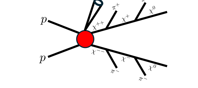
Figure 1: Depiction of a production process for the $5$-plet scenario. Constituent quark / anti-quark annihilation in the protons leads to Drell-Yan production of the pair $\chi^{++}$ and $\chi^{--}$ which subsequently cascade decays to the neutral states $\chi^{0}$. Each subsequent decay emits a pion. This leads to a disappearing track + jet signature.

The $\chi^{\pm}$ state has a mean lifetime given by:

$$\tau=\frac{44\ \text{cm}}{n^{2}-1}.$$ (2.4)

This is long enough for the $\chi^{\pm}$ state to occasionally make it through the pixel detectors of ATLAS or CMS, leaving a track that “disappears” partway through the detector (see figure 2). Disappearing tracks are not included in standard event reconstruction, so at the LHC one needs to trigger on some other kind of visible object. To correctly trigger on this scenario, we also assume the presence of at least one sufficiently hard jet from initial state radiation. This will result in missing transverse momentum that can be triggered on. The disappearing track + $E_{T}^{\mathrm{miss}}$ signature turns out to be the most prominent signature found in earlier studies of $n$-plet scenarios [13, 16, 14, 22], and so we also adopt this as our primary signature. Disappearing track signatures are also used in long-lived chargino searches at ATLAS [26] and CMS [27]. Indeed, we shall recast the ATLAS wino search to set a limit on the “just $n$-plet” scenario.

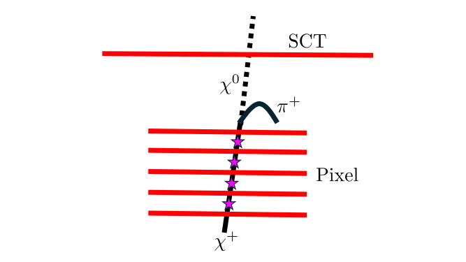
Figure 2: Depiction of $\chi^{+}$ leaving a disappearing track in the Pixel (four hits indicated by the purple stars). It decays into a soft $\pi^{+}$ (circular arc) which is not seen, and to a $\chi^{0}$ (dashed line) which is also not detected. SCT is the microstrip semi-conductor tracker. The disappearing track search requires the $\chi^{\pm}$ to decay before reaching it.

ATLAS Signature

The ATLAS long-lived chargino search looks for charginos produced either through Drell-Yan or from intermediate gluinos. The primary difference between the signal topology of these channels is that the gluino channel expects greater jet multiplicity from the gluino decay, while the electroweak channel needs at least one jet from initial state radiation (ISR). Our “just $n$-plet” scenario necessarily only involves the electroweak channel. We will summarize the electroweak production mode signal region criteria and then summarize the definition of a disappearing track.

The missing transverse energy ($E_{T}^{\mathrm{miss}}$) trigger threshold was set between 70 GeV and 110 GeV depending on the data-taking period. Further selection cuts are applied to distinguish signal from background, and are summarized in table 1.

Signal Region Criteria	Cuts
Number of electrons and muons	0
Number of disappearing tracks	$\geq 1$
$E_{T}^{\mathrm{miss}}$ [GeV]	¿ 200
Number of jets ($p_{T}$ ¿ 20 GeV)	$\geq$ 1
Leading jet $p_{T}$ [GeV]	¿ 100
$\Delta\phi^{\text{jet}-E_{T}^{\mathrm{miss}}}_{\text{min}}$	¿ 1.0

Table 1: ATLAS electroweak production signal region criteria [26]

Before summarizing the disappearing track criteria, some knowledge of the detector geometry is useful. The innermost detector is the pixel silicon detector (referred to as “Pixel”). The barrel region of the Pixel consists of four layers and covers a radius of 33.3 mm to 122.5 mm and a pseudo-rapidity region of $\absolutevalue{\eta}<1.9$. The ATLAS search requires the chargino to traverse through the entire pixel detector, but it must decay before the microstrip semiconductor tracker (SCT) at 30 cm. Further out in radius are the calorimeters and muon spectrometer.

We now summarize the disappearing track cuts. Some straightforward conditions one imposes are:

• 4 hits in the Pixel, none in the SCT

• Small impact parameter

• Isolation from other objects in the event

We comment that there are also more non-trivial cuts having to do with isolating the disappearing track from calorimeter deposits. See Appendix C for a list of the different criteria imposed for the disappearing track search. We comment that similar criteria are applied in the analogous CMS search (see [27] for details), so for ease of exposition we focus primarily on just the ATLAS case.

3 Simulation and Analysis

Let us now turn to the details of our simulation and analysis procedure. We utilized FeynRules [28] to generate a model file describing the particles and their interactions. Madgraph5 [29] was used for the LO matrix element calculation. The 130 NNPDF23LO PDF was used and read by LHAPDF6 [30]. Events were showered and hadronized in Pythia8 [31]. Up to two additional partons were generated in Madgraph5, and events were matched utilizing the MLM matching procedure [32, 33]. Jets were clustered using FastJet [34] with the shower-kt algorithm.

Delphes [35] was used to simulate reconstruction with the default ATLAS card. Though Delphes only propagates final-state particles through its simulation and does not simulate the inner trackers or propagate our $\chi^{\pm}$ state, it is used to simulate reconstruction for the other objects in the event.

To apply the disappearing track cuts, we use the generator-level output from Pythia. Additionally, ATLAS provides a SimpleAnalysis [36] implementation of the disappearing track search. Though we could not use this directly, we were able to use the provided efficiency maps for the disappearing track reconstruction efficiency and missing energy trigger trigger efficiency. The disappearing track efficiency map provides acceptance $\times$ efficiency for cuts we are not able to apply ourselves, such as a chi-squared-goodness of fit score. The missing transverse energy trigger efficiency map provides efficiencies for the trigger parameterized in jet energy and missing transverse energy.

Utilizing both the Delphes and Pythia output, we applied the event selection cuts and disappearing track cuts to each event. Once a final number of events was attained we scaled the final number of events to match the appropriate effective luminosity of 136 $\mathrm{fb}^{-1}$. A similar procedure can be carried out to produce limits at higher luminosity.

4 Results

To obtain limits on the just $n$-plet scenarios, we recast the results of the ATLAS disappearing-track search for winos [26]. Although motivated by the presence of such a state in the MSSM, one can understand the “electroweak channel” minimally as testing the possibility of a new $SU(2)$-triplet fermion augmenting the Standard Model. It is straightforward to extend the analysis to the higher-dimension representations of $SU(2)_{L}$ that challenge the existence of string theory.

The ATLAS search designates control and validation regions for a data-determined number of background events in their signal region. This number, along with its uncertainty, is compared with the data in a classic “cut-and-count” search utilizing the $CL_{s}$ method to place a limit on the wino mass. As detailed in Section 3, for our multiplets of interest we scan in mass to generate a number of events that we then subject to the ATLAS cuts and acceptance $\times$ efficiency for observing disappearing tracks. For each model point, we thus predict a number of events that would appear in the signal region. From this, we can perform our own $CL_{s}$ analysis to place an estimated limit on the BSM particle mass.

For the background-only hypothesis, having observed $n_{\text{obs}}$ events, we construct the likelihood as

$$L_{\text{B}}=\int_{0}^{\infty}\frac{(b^{\prime})^{n_{\text{obs}}}e^{-b^{\prime}}}{n_{\text{obs}}!}\pi_{b}(b^{\prime},\Delta b)\,db^{\prime}.$$ (4.1)

The function $\pi_{b}$ is a probability distribution function (PDF) given by a truncated, normalized Gaussian which peaks at the expected number of background events in the signal region provided by ATLAS, $b$. Its width, $\Delta b$ is the reported uncertainty on this number. In this way, the expected number of background events $b^{\prime}$ in the Poisson factor is integrated over as a nuisance parameter.

Similarly, for the signal plus background hypothesis,

$$L_{\text{S+B}}=\int_{0}^{\infty}\int_{0}^{\infty}\frac{(s^{\prime}+b^{\prime})^{n_{\text{obs}}}e^{-(s^{\prime}+b^{\prime})}}{n_{\text{obs}}!}\,\pi_{s}(s^{\prime},\Delta s)\pi_{b}(b^{\prime},\Delta b)\,ds^{\prime}\,db^{\prime}.$$ (4.2)

We again convolve with a truncated-Gaussian PDF $\pi_{s}$, though the determination of $\Delta s$, the uncertainty on the expected number of signal events, is more involved. There is a systematic uncertainty due to detector and analysis effects that we take from the ATLAS paper. There is a theoretical uncertainty in the computed cross section for our model that we take from Madgraph5. Lastly, there is a statistical uncertainty due to the finite number of events that we generate. To minimize this, we typically run more than 10$\times$ the number of events that would have appeared in the ATLAS data sample. The three contributions to $\Delta s$ are added in quadrature. We summarize our signal and background parameters in table 2.

Multiplet	$b$	$\Delta b$	$n_{\text{obs}}$	$s$	$\Delta s_{\text{tot.}}$	$\Delta s_{\text{syst.}}$	$\Delta s_{\text{theo.}}$	$\Delta s_{\text{stat.}}$
All	3.0	0.7	3	-	$0.11\,s$	-	-	-
3	”	”	”	3.96	0.33	0.28	0.003	0.18
5	”	”	”	3.48	0.40	0.18	0.002	0.38
7	”	”	”	7.10	1.52	0.31	0.003	1.49
9	”	”	”	4.29	2.28	0.43	0.003	2.25

Table 2: Parameters used in $CL_{s}$ analysis. The representation-independent ones are taken from [26]. The numbers of signal events and their uncertainties given are for the mass closest to the limit for that representation. For the breakdown of $\Delta s$ into its various components, we take the quadrature sum of each type across production channels.

Following the $CL_{s}$ method, we obtain the 95% CL limit on particle mass for each representation from the log-likelihood ratio. Specifically, we compute

$$\lambda(\mu)\equiv-2\log\left(\frac{L_{\text{S+B}}(\mu)}{L_{\text{B}}}\right),$$ (4.3)

where $\mu$ is a factor that multiplies $s$ where it appears in $L_{\text{S+B}}$ in equation (4.2), including the $s$-dependent contributions to $\Delta s$. We then solve for the $\mu$ value when $\lambda(\mu)=-2.71$. If $\mu>1$, then that mass point is still viable, and conversely for $\mu<1$. Scanning masses in 25 GeV increments, in table 3 we report the lower bound on mass for each multiplet.

There are a few qualitative comments to make on this recast analysis. First of all, we observe that in our simulation of the $3$-plet, our limit of $725$ GeV is somewhat more aggressive than that set by ATLAS ($660$ GeV, see [26]). The most likely explanation for this discrepancy is either a difference in simulating detector effects and / or the construction of the likelihood function. We find it encouraging, however, that the limit obtained from our cruder simulation efforts is within $\sim 70$ GeV of the experimentally quoted answer. Similar considerations hold for the CMS limit of $650$ GeV (see [27]).

The next comment concerns the overall dependence on the mass limit as a function of $n$, the dimension of the representation. Observe that the production cross section scales with $n^{2}$, leading to significantly more events. On the other hand, the decay rate also increases, shortening the length of the disappearing track. A second comment here is that only a tail of the momentum distribution for such decays is actually observable; at higher $n$ one is even further out on the tail of the distribution. The combined effect is a reduced limit as one increases $n$. This is not so pronounced for $n=3,5,7$, but for $n=9$ the limit we can set is somewhat lower ($400$ GeV).

Multiplet	ATLAS (recast)	ATLAS [26]
3	735	660
5	675	-
7	625	-
9	400	-

Table 3: 95% CL limits on the mass in GeV of a new electroweak multiplet added in isolation to the Standard Model. For the triplet, we report the limits obtained by a recent ATLAS analysis. We then provide our results from recasting these limits. We scan in mass in 25 GeV steps and report that lowest mass whose test statistic pass the 95% CL.

Going forward, the high-luminosity LHC will make further progress on these searches. It is beyond our scope to provide a detailed projection of the scaling of backgrounds in a cut-and-count analysis. Instead, for the ATLAS results, we show in table 4 three different scenarios for 3 ab^-1 of data for how the background will scale. If the increase in the number of background events is worse than a 50% increase over the ratio of luminosities, then our simple cut & count analysis will not set limits substantially stronger than the current ones. Such a scenario would motivate innovation on the analysis side to deal with this more challenging experimental environment. For example, one could use precision Drell-Yan measurements at large invariant mass and high-luminosity to determine the running of $\alpha_{2}$ to improve limits on representations with $n\gtrsim 7$ beyond those given in table 4 [37, 38].

Multiplet	$\propto\mathcal{L}$	$\mu$	$\propto\mathcal{L}\times$1.25	$\propto\mathcal{L}\times$1.5
3	800	1.47	800	800
5	800	1.06	775	750
7	650	1.43	625	625
9	475	1.27	475	475

Table 4: Projected 95% CL limits on the mass in GeV for the high-luminosity LHC at 3 ab^-1, extrapolating from the ATLAS study with 136 fb^-1. The columns label how we scaled the number of background events relative to the increase in luminosity. We scan in mass in 25 GeV steps and report that lowest mass whose test statistic pass the 95% CL. For the case where the background just scales with luminosity, we also give the $\mu$ value, which scales up the number of signal events to reach 95% exclusion.

In figure 3, we plot the limits from both the recast analysis of [26] and our projection to the high-luminosity LHC.

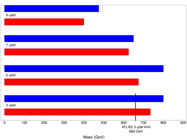
Figure 3: 95% CL limits on masses for four “just $n$-plet” scenarios at the LHC. The recast limits from the ATLAS disappearing track search [26] are in red, and our projected limits for a 3 ab^-1 run of the high-luminosity LHC are in blue. The latter represent the column in table 4 that assumes the background scales exactly with luminosity.

5 Discussion

In this work we have studied a class of phenomenological scenarios which is extremely challenging, if not outright impossible to realize in string theory. The main point is that the phenomenologically well-motivated “just an $n$-plet of $SU(2)_{L}$” scenario is very hard / impossible to engineer. We do not (yet) have a no-go theorem, but there are good reasons to believe that this sort of model would pose fatal challenges for string-based model building. An additional outcome of our analysis is an updated set of current LHC limits on just $n$-plet scenarios. Let us turn to some natural extensions of the present work.

We have primarily focused on setting exclusion limits for the “just an $n$-plet of $SU(2)_{L}$” scenario. Conversely, suppose we indeed observe an excess number of events. The inverse problem of determining the $n$-plet mass $M$, as well as the specific value of $n$ would clearly be an important task, since $n\geq 5$ does not arise in string theory. The measurable trio of particle mass, decay length, and production rate would strongly constrain the possible value of $n$. Other signatures / search strategies can then be used to distinguish between these possibilities. It would be exciting to investigate this question further.

On the formal side, it would of course be desirable to have a complete no-go theorem that the “just $n$-plet” scenario cannot be realized in string theory. While this would appear to require a deep knowledge of non-perturbative quantum gravity, all indications point to this scenario being ruled out. As a more concrete near-term goal, one might hope to prove that no perturbative string theory can realize such a scenario. Complementary to this, sharpening constraints on the mass spectrum of strongly coupled quantum field theories would also rule out scenarios in which the $n$-plet emerges as a composite state.

On the observational side, the next decade looks to be especially promising for testing the possibility that a simple $SU(2)_{L}$ $n$-plet is the lowest-lying state beyond the weak scale. There are updated direct and indirect dark matter detection experiments on the horizon, and future colliders such as a proposed muon collider or high energy hadronic facility would all provide improved bounds and limits on this class of scenarios.

A further comment is that here we have focused on a specific, quite minimal extension of the Standard Model. One can envision widening our scope to bosonic states with the same representation content, as well as far more general states in high-dimensional representations of the Standard Model gauge group. One can also envision more intricate interactions which lead to distinctive signatures. Again, the key point is that a positive detection for any such scenario would amount to ruling out the entire (known) string landscape.

More broadly speaking, we believe it is important to develop phenomenological scenarios which—if detected—would falsify the (known) string landscape. Indeed, the value of a theory lies not just in its predictions, but also in what it cannot accommodate.

Appendix A Electroweak $n$-plet of $SU(2)_{L}$

In this Appendix we briefly review some aspects of an $n$-plet of $SU(2)_{L}$. We consider both the case of a Dirac $(c=1)$ and Majorana $(c=1/2)$ particle in a real $n$-dimensional representation. To set notation, we denote by $T^{a}$ the Lie algebra generators for $\mathfrak{su}(2)_{L}$, i.e., $[T^{a},T^{b}]=i\varepsilon^{abc}T^{c}$. We also introduce the standard raising and lowering operators for $\mathfrak{su}(2)_{L}$, i.e. $T^{\pm}=T^{1}\pm iT^{2}$.

By inspection, we observe that the electroweak bosons interact with the $\chi$ particles:

$$\mathcal{L} \supset c\frac{g}{\sqrt{2}}\overline{\chi}W_{\mu}^{+}\gamma^{\mu}T^{+}\chi=c\sqrt{j(j+1)-m(m+1)}\left(\overline{\chi}_{m+1}\gamma^{\mu}\chi_{m}\right)\frac{gW_{\mu}^{+}}{\sqrt{2}}$$ (A.1)

$$\mathcal{L} \supset c\frac{g}{\sqrt{2}}\overline{\chi}W_{\mu}^{-}\gamma^{\mu}T^{-}\chi=c\sqrt{j(j+1)-m(m-1)}\left(\overline{\chi}_{m-1}\gamma^{\mu}\chi_{m}\right)\frac{gW_{\mu}^{-}}{\sqrt{2}}$$ (A.2)

$$\mathcal{L} \supset cg\overline{\chi}A_{\mu}^{3}\gamma^{\mu}T^{3}\chi=cm\left(\overline{\chi}_{m}\gamma^{\mu}\chi_{m}\right)\left(\frac{g}{\cos\theta_{W}}Z_{\mu}^{0}+eA_{\mu}\right),$$ (A.3)

where in the above we used the explicit matrix representatives for the $\mathfrak{su}(2)_{L}$ generators, $\cos\theta_{W}=g/\sqrt{g^{2}+g^{\prime 2}}$, and $e=g\sin\theta_{W}$.

Much of the phenomenology of the scenario is dictated by the mass splitting within the $n$-plet, as well as the resulting decay rate to each subsequent member of the multiplet. Observe that in the absence of electroweak symmetry breaking, all components of the multiplet have the same mass. After electroweak symmetry breaking, radiative corrections from the vector bosons generate a mass splitting between the different components. In [13] the mass splittings were studied in general. In particular, in the limit where $M/M_{W,Z}\gg 1$, the mass splitting between different electric charge components of the multiplet have a simple form:

$$M_{Q}-M_{Q^{\prime}}\simeq\left(Q^{2}-Q^{{}^{\prime}2}\right)\frac{\alpha_{2}s_{W}^{2}}{2}M_{W}\simeq\left(Q^{2}-Q^{{}^{\prime}2}\right)\times 166\text{ MeV.}$$ (A.4)

The bottom component of the multiplet is stable against further decay (there is a $\mathbb{Z}_{2}$ symmetry which protects it), but the higher components of the multiplet are expected to eventually cascade decay down to this lightest state. On the timescale of collider signatures, the charge $|Q|>1$ states decay within the inner tracker. However, the final charged state decays to the neutral component with the following rates and branching ratios [13]:

$$\Gamma(\chi^{+} \rightarrow\pi^{+}\chi^{0})=\left(n^{2}-1\right)\frac{G_{F}^{2}V_{ud}^{2}\left(\Delta M\right)^{3}f_{\pi}^{2}}{4\pi}\sqrt{1-\left(\frac{M_{\pi}}{\Delta M}\right)^{2}}\text{ \ }(\text{BR}\sim 97.7\%)$$ (A.5)

$$\Gamma(\chi^{+} \rightarrow e^{+}\nu_{e}\chi^{0})=\left(n^{2}-1\right)\frac{G_{F}^{2}\left(\Delta M\right)^{5}}{60\pi^{3}}\text{ \ }(\text{BR}\sim 2.05\%)$$ (A.6)

$$\Gamma(\chi^{+} \rightarrow\mu^{+}\nu_{e}\chi^{0})=0.12\times\Gamma(\chi^{+}\rightarrow e^{+}\nu_{e}\chi^{0})\text{ \ }(\text{BR}\sim 0.25\%).$$ (A.7)

For example, this leads to a rest-frame lifetime of the $\chi^{+}$ from the quintuplet of $\approx 0.06$ ns, which can easily give a macroscopic decay length.

Appendix B Stringy High-Dimensional Representations

In this Appendix we provide some additional details on why high-dimensional representations are difficult—though not impossible—to realize in string theory. Additionally, we motivate the conjecture that the “just $n$-plet of $SU(2)_{L}$” scenario cannot be realized. We focus on the case where the new state is a fermion, but comment that quite similar considerations hold for new bosonic states as well. Indeed, in supersymmetric models one often has both sorts of states anyway.

There are two constraints we need to impose right from the start. First, we need to have a gauge group which can accommodate the standard electroweak doublets, so a gauge group such as $SO(3)$ will not work. Second, we need to find matter in the $n$-plet of $SU(2)_{L}$ for some $n\geq 5$. As throughout, we take $n$ to be odd (i.e., real rather than pseudo-real representations) so there is no constraint from anomalies. There are two well-substantiated conjectures that we put forward:

• No (known) stringy Standard Model has $n\geq 5$ matter

• Adding just the $n$-plet for $n\geq 5$ is not possible in string theory

In both cases, our discussion falls short of a no-go theorem, but the state of the art suggests that both claims are quite plausible.

To begin, we review some of the canonical approaches to realizing matter representations via perturbative open and closed string theories, as well as their extensions to strongly coupled regimes.

After this, to illustrate some of the relevant issues, we also discuss how one can use strongly coupled dynamics to build bound states with high-dimensional representations. Such scenarios can be implemented in many stringy setups, but fitting this with various qualitative phenomenological constraints is far more challenging. Additionally, in all the examples we encounter, one finds not just the $n$-plet of $SU(2)_{L}$ but also lower-dimensional representations such as the triplet which are lighter or nearby in mass. Motivated by these considerations, we then give a more precise sense in which models such as the “just $n$-plet scenario” for $n\geq 5$ do not arise in string theory.

B.1 Matter with Open Strings

To begin, we start by discussing how stringy Standard Models arise via open strings. We begin by working with perturbative open strings and then extend our discussion to the case of strongly coupled bound states. Recall that in a perturbative open string, there are two endpoints and these can be decorated by an additional Chan-Paton factor. These endpoints should be viewed as terminating on a Dirichlet brane (D-brane). Each such Chan-Paton factor indicates a single fundamental index of a corresponding gauge group. For example, an open string which stretches from a single stack back to itself can support gauge fields in the adjoint representation. Allowing for orientation reversal of open strings, this general construction allows one to realize all of the classical Lie algebras, namely $SU(N)$, $SO(N)$ and $Sp(N)$ (as well as $U(1)$ factors). Since open strings carry two endpoints, we also see that the sorts of matter fields (spin $0$ and spin $1/2)$ which can be accommodated in this approach consist of two-index representations of a single gauge group. For example, for $SU(N)$ this consists of the adjoint representation as well as the two-index symmetric and anti-symmetric representations. Similar considerations hold for the other classical Lie algebras. One can also achieve matter in a single index representation by considering bifundamental representations for products of two simple gauge groups $G_{1}\times G_{2}$. We interpret this as an open string which stretches between two stacks of D-branes. Note in particular that matter in the $\mathbf{5}$ of $SU(2)$ would have required a 4-index symmetric representation. The essential point we draw from these considerations is that at least at the level of perturbative open strings, the sorts of matter representations which can actually be realized are rather limited; we have matter fields in either a single index or two index representation. See figure 4 for a depiction.

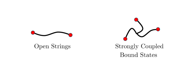
Figure 4: Depiction of a perturbative open string, as well as a strongly coupled bound state of open strings. The available representations which can be built with perturbative open strings are limited to one- and two-index representations; the indices can be associated with the endpoint of the strings. At strong coupling one can in principle form additional bound states associated with multi-prong string configurations. Even so, the range of options is quite limited.

Of course, there are well-known limitations to working with perturbative open strings. For example, even the possible gauge groups which can be realized in this way excludes all of the exceptional Lie algebras as well as important ingredients such as the spinor representation of $SO(N)$. In type IIB string theory these more general possibilities can all be realized by working in terms of non-perturbative bound states of strings known as string junctions. One then considers not just the fundamental string (F1-string), but also its S-dual the D1-brane (D1-string) and dyonic bound states of these strings known as $(p,q)$ strings. For our present considerations, the essential point is that such bound states lead to string junctions with more than two endpoints. As such, this provides a promising route to realizing representations with more indices. References [44, 45] explicitly show how to realize the exceptional Lie algebras and some representations in terms of such string junctions (see also [46]).

To illustrate, consider matter in the $\mathbf{78}$ of $E_{6}$, namely the adjoint representation of $E_{6}$. One can now realize representations such as the $\mathbf{20}$ of $SU(6)$, i.e., the three-index anti-symmetric of $SU(6)$ via the decomposition:

$$E_{6} \supset SU(6)\times SU(2)$$ (B.1)

$$\mathbf{78} \rightarrow(\mathbf{35},\mathbf{1})+(\mathbf{1},\mathbf{3})+(\mathbf{20},\mathbf{2}).$$ (B.2)

Such breaking patterns are also straightforward to realize in M-theory and F-theory backgrounds. In this setting, one begins with a higher-dimensional gauge theory which also includes adjoint valued matter. Working with backgrounds where the adjoint valued matter and the gauge fluxes are switched on then produces breaking patterns which can reproduce many of the successful breaking patterns used in purely 4D GUTs (often with fewer model building complications). See e.g., [52, 53, 54, 55, 56] as well as the reviews [57, 58, 59].

One of the subtle points in this method is that accommodating the gauge group of the Standard Model typically imposes rather strong restrictions on realistic breaking patterns. For example, one of the best-motivated routes to realizing the Standard Model factors through an intermediate GUT group. To illustrate, we start with the $\mathbf{248}$ of $E_{8}$, i.e., the adjoint representation of $E_{8}$ and consider the decomposition first to $SU(5)_{\text{GUT}}\times SU(5)_{\bot}$:

$$E_{8} \supset SU(5)_{\text{GUT}}\times SU(5)_{\bot}$$ (B.3)

$$\mathbf{248} \rightarrow(\mathbf{24},\mathbf{1})+(\mathbf{1},\mathbf{24})+(\mathbf{5},\overline{\mathbf{10}})+(\overline{\mathbf{5}},\mathbf{10})+(\mathbf{10},\mathbf{5})+(\overline{\mathbf{10}},\overline{\mathbf{5}}),$$ (B.4)

where the $\mathbf{5}$ denotes the fundamental representation (single index) and the $\mathbf{10}$ denotes the two-index anti-symmetric representation. As is well known, this suffices to reach the representation content present in the Standard Model, but it does not support more exotic representations such as the $\mathbf{5}$ of $SU(2)_{L}$.

To date, the vast majority of realizations of the Standard Model within string theory actually proceed via such low-dimensional representations, i.e., either through perturbative open string constructions or via a GUT group breaking pattern as in line (B.3) - (B.4). In principle one could contemplate a more exotic embedding of the Standard Model gauge group in $E_{8}$. For example, one could consider the diagonal embedding of $SU(5)_{\text{diag}}\subset SU(5)_{\text{GUT}}\times SU(5)_{\bot}\subset E_{8}$, but even this would not produce a four-index symmetric representation.

Let us also comment that in more exotic F-theory backgrounds with additional tunings / non-geometric ingredients it is sometimes possible to engineer more exotic representations (see e.g., [7, 8, 10] as well as the comments in [11]), but even so, engineering the $\mathbf{5}$-plet as part of a Standard Model gauge group has (to date) not been realized.

The general point we make here is that in the context of building stringy Standard Model-like vacua with high-dimensional representations, engineering the $\mathbf{5}$-plet of $SU(2)_{L}$ appears challenging / impossible via this route.

B.2 Matter with Closed Strings

Historically the first examples of string backgrounds which include the Standard Model gauge group were generated via perturbative closed strings, i.e., the $E_{8}\times E_{8}$ heterotic string [61, 62, 63, 64]. In this setting, the vast majority of semi-realistic backgrounds arise from a 2D worldsheet CFT in which the $E_{8}$ is generated via a 2D current algebra. In the target space this appears as a 10D super Yang-Mills theory sector, which is subsequently compactified to produce the relevant gauge groups and matter content of the Standard Model. In this case, the same representation theory based restrictions discussed above still apply, leading to rather strong restrictions on the available representation content for matter charged under the Standard Model gauge group.

Broader possibilities are available, however, since one can in principle consider a more general 2D CFT current algebra. Here, the main idea is that global symmetries of the 2D worldsheet CFT inevitably become gauge symmetries in the target space. In particular, we are interested in models where the worldsheet has an $SU(2)_{L}$ global symmetry.

A particularly well-studied example involves higher Kac-Moody levels, as in references [65, 66, 67, 68]. The key feature of these constructions is that one can in principle realize low dimension conformal primary operators in high-dimensional representations. As such, these states can in principle be part of the massless spectrum of a string background.

To illustrate, consider a putative chiral $SU(2)$ current algebra at level $k\in\mathbb{Z}_{>0}$. The central charge of this CFT sector is:

$$c=\frac{3k}{k+2}\leq 3,$$ (B.5)

where the upper bound is only saturated at $k\rightarrow\infty$ (a classical background). A primary operator in a spin$-j$ representation of $SU(2)$ has weight:

$$h_{j}=\frac{j(j+1)}{k+2},$$ (B.6)

and so in principle we can have very large values of $j$ with low weight. It is worth noting here that this sort of construction only provides a set of candidate massless states in a given string spectrum. Indeed, to get a massless state we need the total conformal weight to be exactly one. One can accomplish this by assuming that the worldsheet CFT contains another sector so that the actual operator of interest is of the (schematic) form:

$$\mathcal{O}_{j,\text{full}}=\mathcal{O}_{j}\mathcal{O}_{\text{extra}},$$ (B.7)

so that the total weight $h_{j}+h_{\text{extra}}=1$. If one cannot find such an extra sector and a suitable operator such that the total weight can be raised to one, then one either has a tachyon in the spectrum or one must include a suitable GSO projection to remove the offending state from the low energy spectrum.

Group theoretically, working with Kac-Moody levels leads to non-trivial embeddings of the Standard Model gauge group in a bigger product gauge group structure [66, 67, 68]. We are unaware of an explicit example which contains the Standard Model as well as the $\mathbf{5}$ of $SU(2)_{L}$, but it is plausible that this, or related construction methods based on non-geometric backgrounds (see e.g., asymmetric orbifolds [69, 70]) can yield such states.

That being said, these sorts of constructions appear to always come with matter in a wide variety of representations, including the $\mathbf{3}$ of $SU(2)_{L}$. To see the issue, let us return to equation (B.6). Suppose we have managed to build a model with a massless spin-$j$ representation. Consider next a spin $l<j$ representation. Observe that this has lower weight:

$$l<j\Rightarrow h_{l}<h_{j}.$$ (B.8)

Returning to our discussion near (B.7), we now face the issue of how to remove the $\mathcal{O}_{l}$ operator from the string spectrum. It is not altogether clear whether this can be accomplished since the condition of modular invariance generally requires one to not “thin out” the spectrum of chiral primary operators. There are some known exceptions to these considerations based on maverick coset constructions (see e.g.,[71]) but as far as we are aware there is no known way to get “just the $\mathbf{5}$-plet and nothing else.”

B.3 Building Exotic Representations via Strong Coupling

Having reviewed some variants on open and closed string constructions of representations in Standard Model-like vacua, we now turn to a general method for realizing exotic representations which can be accommodated in explicit string backgrounds. The main feature we wish to stress is that even though we can indeed realize these higher-dimension representations, the resulting scenarios always contain other, lighter states in smaller representations. This is different from the “just $n$-plet” type scenario we have investigated in this work.

The main idea can be stated in bottom up terms: We wish to view the $n$-plet as a composite operator which is really a strongly coupled bound state comprised of “preons” built from lower-dimensional representations. To build explicit examples of high-dimensional representations we consider a generic extra sector in which the SM gauge group appears as a weakly gauged flavor symmetry. See figure 5 for a representative example.

Figure 5: Depiction of quiver / moose diagram where there is a strongly coupled gauge theory with gauge group $SU(N)_{\mathrm{extra}}$ (circle), and in which the $SU(2)_{L}$ factor of the Standard Model gauge group appears as a weakly gauged flavor symmetry (square). The oriented lines connected the two groups are messenger fields in representations of both gauge groups. Strong coupling dynamics in the extra sector can lead to bound states in bigger representations of $SU(2)_{L}$, but generically these are accompanied by towers of states which cannot be decoupled. One can view the connecting lines as open strings which end on different branes used to build the respective gauge groups.

As a warmup, consider $SU(N)$ gauge theory with $N_{f}$ quark flavors. We split the quarks into Weyl fermions and consider left-handed fermionic fields $\psi_{(s,f)}^{g}$ where the label $s$ indicates the spacetime spin, $f$ is an index for the anti-fundamental of $SU(N_{f})$ and $g$ is an index for the fundamental of $SU(N)$. We denote by $\widetilde{\psi}$ the left-handed Weyl fermions in the conjugate representations of the flavor and gauge groups. In this example, there is a gauge invariant baryonic operator:

$$\mathcal{B}=\varepsilon_{g_{1}...g_{N}}\psi_{(s_{1},f_{1})}^{g_{1}}...\psi_{(s_{N},f_{N})}^{g_{N}}.$$ (B.9)

Assuming the theory confines (due to an appropriate choice for the number of flavors) the baryon is a degree of freedom of the low energy effective field theory. Owing to Fermi statistics, the resulting operator is in the $N$-fold fully symmetrized representation:

$$\mathrm{Sym}^{N}\left(\frac{1}{2}\otimes\overline{N_{f}}\right),$$ (B.10)

in the obvious notation. In particular, one can conceive of embedding $SU(2)_{L}$ in the diagonal $SU(N_{f})$ flavor symmetry; adding additional interaction terms can also break $SU(N_{f})_{\mathrm{diag}}$ down to $SU(2)_{L}$. The resulting bound state can thus be used to produce a field in the $N$-fold symmetrized product of $SU(2)_{L}$. Setting $N=4$ would, for example, realize a $\mathbf{5}$-plet of $SU(2)_{L}$. This is not quite what we need, however, because the spacetime spin is also symmetrized, and would also result in a spin $N/2$ mode. It is also worth noting that the baryon constructed in this way is accompanied by many lighter degrees of freedom, including mesons in the adjoint representation of $SU(N_{f})_{\mathrm{diag}}$.

The limitation of this warmup example is that we have introduced many fields which transform in a single big flavor symmetry. This in turn required us to full symmetrize all the flavor and spacetime spin indices simultaneously.

There are many ways to improve on the above situation to produce composite operators with high-dimensional flavor symmetry representations, but with low spacetime spin. As an example, one can consider composite operators built from both spin $1/2$ and spin $0$, as frequently occurs in supersymmetric gauge theories. For example, the scalar “baryon operator” of supersymmetric QCD is instead in the fully anti-symmetric representation of $SU(N_{f})$. This is not quite the representation we want, but it at least goes to the point that we can in principle build bigger representations.

To improve on these constructions, we can consider models in which the diagonal flavor symmetry is instead $SU(2)_{1}\times...\times SU(2)_{K}=SU(2)^{K}$ for some $K>0$, viewing $SU(2)_{L}$ as the diagonal subgroup of $SU(2)^{K}$. Labelling each set of bifundamentals as $\psi^{(i)}$, we can again make composite states but now where the spacetime spin is not correlated with the representation for our flavor symmetry.

A general comment at this point is that in the process of building our desired high-dimension representation, we seem to inevitably encounter other composite states which are in lower-dimension representations of the flavor symmetry. For example, in real world QCD, we have baryons such as the decuplet and octet of $SU(3)_{\mathrm{flavor}}$ but we also have the pions (as members of a different octet), which are significantly lighter. The general expectation, in fact, is that one ought to expect an entire tower of resonances of varying spins and representations.

Building examples with such high-dimensional representations can also be carried out in string-based constructions. For example, in many F-theory constructions where the Standard Model is realized via a stack of intersecting / magnetized 7-branes, we can introduce an extra sector via a probe D3-brane. Examples of strongly coupled extra sectors realized in this fashion include [72, 73, 74, 75]. In this setting, the extra sector will typically support many light degrees of freedom in high-dimensional representations of the Standard Model gauge group; this is in some sense a generic feature of having a conformal field theory (CFT) with a flavor symmetry. There is a priori no reason that the higher-dimensional representations will be accompanied by a high spacetime spin so there is generically no issue with generating many high-dimensional representations.

What then, is the basis of our claim that realizing $n$-plet scenarios is actually difficult / well nigh impossible in string theory? The main point is that in all of these examples the $n$-plet is never in isolation. Rather, it is simply part of a large tower of resonances in a strongly coupled sector that also includes lighter / comparable mass states in lower-dimensional representations. What we are really after, then, is a decoupling limit where all of the other resonances other than the $n$-plet can be decoupled from the spectrum.

This is far more challenging to arrange. To illustrate some of the issues one confronts in trying to decouple everything but an $n$-plet, it is helpful to keep in mind the QCD inequalities for a vectorlike gauge theory. In this case, positivity of the path integral measure in Euclidean signature leads to rather stringent constraints on the relative masses of the pions and baryons, and similar considerations are expected to hold for more “exotic” representations of the flavor symmetry of the sort of relevance to us. The main lesson in these theorems is that the pion ends up being lighter than the baryon. As such, the “just $n$-plet” scenario is actually not realized by such vectorlike theories. A related comment is that insofar as the baryons of a QCD-like theory can be treated as solitonic excitations, namely skyrmions, they must necessarily be heavier than the pions of the theory. It also runs counter to large $N$ counting arguments of the sort presented in [88].

In this regard an interesting situation to consider is that of supersymmetric QCD with $N_{f}=N_{c}+1$ flavors. In this case, the existence of a baryonic and mesonic branch for the moduli space [89] means that at least in this limit, the baryons and mesons of SQCD are both exactly massless. In principle adding a non-supersymmetric mass term for the squarks could lift this degeneracy, and a priori one could imagine the baryon being lighter than the pion. See for example [90, 91] for some discussion of such non-supersymmetric deformations. Even so, it seems rather implausible that in these scenarios one can fully decouple the other representations. Said differently, all of these states are still filling out a tower of states and cannot be decoupled from one another.

An additional comment here is that in the related examples discussed above where we considered strongly coupled bound states of open strings (in IIB / F-theory) as well as higher Kac-Moody level constructions, the bottom up characterization of such states inevitably appears to involve a compositeness scale of some kind. Of course, in these latter examples the compositeness scale is all the way up at the string scale, but from a bottom up perspective one can consider taking this far lower, and this appears to also be realizable in string constructions (as we have just shown).

Summarizing, while it is in principle possible to realize high-dimensional representations in string constructions, we are not aware of any example which includes the Standard Model as a subsector. Further, in approaches to realizing an $n$-pet of $SU(2)_{L}$ with $n\geq 5$, we inevitably appear to encounter a whole tower of extra states including those in lower-dimensional representations.

This, of course, falls short of an actual no-go theorem, but all of the evidence points to this being an extremely challenging scenario to accommodate. Said differently, detection of the “just $n$-plet scenario” would eliminate the entire known landscape of string vacua.

Appendix C ATLAS Criteria for Disappearing Track Search

In this Appendix we briefly list the ATLAS criteria for their disappearing track search [26]:

1. Pseudo-rapidity in the range: $0.1<\absolutevalue{\eta}<1.9$

2. Hits in 4 consecutive Pixel layers and none in the SCT

3. $p_{T}>20$ GeV

4. Longitudinal impact parameter: $\absolutevalue{d_{0}/\text{err}\quantity(d_{0})}$ ¡ 1.5

5. Transverse impact parameter: $\absolutevalue{z_{0}^{\text{HS}}}\sin{\theta}$ ¡ 0.5 mm

6. The deviation between the measured data and the tracklet fits lies within a likelihood of $10\%$, given the tracklet. That is the chi-squared probability $\quantity(\chi^{2},\text{ndf})$ ¿ 0.1.

7. Isolation from other tracks in the event. The sum of standard track momenta in a cone of $\Delta R=0.4$ about the disappearing track must be less than $4\%$ of the disappearing track momenta: $p_{T}^{\text{cone}40}/p_{T}<0.04$

8. Isolation from calorimeter deposits. The sum of transverse energy in a cone of $\Delta R=0.2$ about the disappearing track must be less than 5 GeV: $E_{T}^{\text{topoclus20}}$ ¡ 5 GeV

9. Overlap removal, discard event if an electron or muon is within $\Delta R=0.4$ of the disappearing track

In our own simulation we implement items 1, 3, 8, and 9.

References

- [1] M. R. Douglas and S. Kachru, “Flux compactification,” Rev. Mod. Phys. 79 (2007) 733–796, arXiv:hep-th/0610102.
- [2] F. Denef, “Les Houches Lectures on Constructing String Vacua,” Les Houches 87 (2008) 483–610, arXiv:0803.1194 [hep-th].
- [3] R. Bousso and J. Polchinski, “Quantization of four form fluxes and dynamical neutralization of the cosmological constant,” JHEP 06 (2000) 006, arXiv:hep-th/0004134.
- [4] M. Dine, “Naturalness Under Stress,” Ann. Rev. Nucl. Part. Sci. 65 (2015) 43–62, arXiv:1501.01035 [hep-ph].
- [5] B. S. Acharya and M. R. Douglas, “A Finite landscape?,” arXiv:hep-th/0606212.
- [6] J. J. Heckman and C. Vafa, “Fine Tuning, Sequestering, and the Swampland,” Phys. Lett. B 798 (2019) 135004, arXiv:1905.06342 [hep-th].
- [7] C. Lüdeling and F. Ruehle, “F-theory duals of singular heterotic K3 models,” Phys. Rev. D 91 no. 2, (2015) 026010, arXiv:1405.2928 [hep-th].
- [8] D. Klevers, D. R. Morrison, N. Raghuram, and W. Taylor, “Exotic matter on singular divisors in F-theory,” JHEP 11 (2017) 124, arXiv:1706.08194 [hep-th].
- [9] N. Raghuram and W. Taylor, “Large U(1) charges in F-theory,” JHEP 10 (2018) 182, arXiv:1809.01666 [hep-th].
- [10] M. Cvetič, J. J. Heckman, and L. Lin, “Towards Exotic Matter and Discrete Non-Abelian Symmetries in F-theory,” JHEP 11 (2018) 001, arXiv:1806.10594 [hep-th].
- [11] W. Taylor and A. P. Turner, “Generic matter representations in 6D supergravity theories,” JHEP 05 (2019) 081, arXiv:1901.02012 [hep-th].
- [12] F. Marchesano, G. Shiu, and T. Weigand, “The Standard Model from String Theory: What Have We Learned?,” Ann. Rev. Nucl. Part. Sci. 74 (2024) 113–140, arXiv:2401.01939 [hep-th].
- [13] M. Cirelli, N. Fornengo, and A. Strumia, “Minimal dark matter,” Nucl. Phys. B 753 (2006) 178–194, arXiv:hep-ph/0512090.
- [14] E. Del Nobile, R. Franceschini, D. Pappadopulo, and A. Strumia, “Minimal Matter at the Large Hadron Collider,” Nucl. Phys. B 826 (2010) 217–234, arXiv:0908.1567 [hep-ph].
- [15] L. Di Luzio, R. Gröber, J. F. Kamenik, and M. Nardecchia, “Accidental matter at the LHC,” JHEP 07 (2015) 074, arXiv:1504.00359 [hep-ph].
- [16] B. Ostdiek, “Constraining the minimal dark matter fiveplet with LHC searches,” Phys. Rev. D 92 (2015) 055008, arXiv:1506.03445 [hep-ph].
- [17] L. Di Luzio, R. Gröber, and G. Panico, “Probing new electroweak states via precision measurements at the LHC and future colliders,” JHEP 01 (2019) 011, arXiv:1810.10993 [hep-ph].
- [18] A. Belyaev, S. Prestel, F. Rojas-Abbate, and J. Zurita, “Probing dark matter with disappearing tracks at the LHC,” Phys. Rev. D 103 no. 9, (2021) 095006, arXiv:2008.08581 [hep-ph].
- [19] S. Bottaro, A. Strumia, and N. Vignaroli, “Minimal Dark Matter bound states at future colliders,” JHEP 06 (2021) 143, arXiv:2103.12766 [hep-ph].
- [20] M. Baumgart, N. L. Rodd, T. R. Slatyer, and V. Vaidya, “The Quintuplet Annihilation Spectrum,” arXiv:2309.11562 [hep-ph].
- [21] M. Cirelli, F. Sala, and M. Taoso, “Wino-like Minimal Dark Matter and future colliders,” JHEP 10 (2014) 033, arXiv:1407.7058 [hep-ph]. [Erratum: JHEP 01, 041 (2015)].
- [22] T. Han, S. Mukhopadhyay, and X. Wang, “Electroweak Dark Matter at Future Hadron Colliders,” Phys. Rev. D 98 no. 3, (2018) 035026, arXiv:1805.00015 [hep-ph].
- [23] R. Capdevilla, F. Meloni, R. Simoniello, and J. Zurita, “Hunting wino and higgsino dark matter at the muon collider with disappearing tracks,” JHEP 06 (2021) 133, arXiv:2102.11292 [hep-ph].
- [24] S. Bottaro, D. Buttazzo, M. Costa, R. Franceschini, P. Panci, D. Redigolo, and L. Vittorio, “Closing the window on WIMP Dark Matter,” Eur. Phys. J. C 82 no. 1, (2022) 31, arXiv:2107.09688 [hep-ph].
- [25] M. Baumgart, S. Bottaro, D. Redigolo, N. Rodd, and T. R. Slatyer, “Testing Real WIMPs with CTAO,” in preparation .
- [26] ATLAS Collaboration, G. Aad et al., “Search for long-lived charginos based on a disappearing-track signature using 136 fb-1 of pp collisions at = 13 TeV with the ATLAS detector,” Eur. Phys. J. C 82 no. 7, (2022) 606, arXiv:2201.02472 [hep-ex].
- [27] CMS Collaboration, A. Hayrapetyan et al., “Search for supersymmetry in final states with disappearing tracks in proton-proton collisions at s=13 TeV,” Phys. Rev. D 109 no. 7, (2024) 072007, arXiv:2309.16823 [hep-ex].
- [28] A. Alloul, N. D. Christensen, C. Degrande, C. Duhr, and B. Fuks, “FeynRules 2.0 - A complete toolbox for tree-level phenomenology,” Comput. Phys. Commun. 185 (2014) 2250–2300, arXiv:1310.1921 [hep-ph].
- [29] J. Alwall, P. Demin, S. de Visscher, R. Frederix, M. Herquet, F. Maltoni, T. Plehn, D. L. Rainwater, and T. Stelzer, “MadGraph/MadEvent v4: The New Web Generation,” JHEP 09 (2007) 028, arXiv:0706.2334 [hep-ph].
- [30] A. Buckley, J. Ferrando, S. Lloyd, K. Nordström, B. Page, M. Rüfenacht, M. Schönherr, and G. Watt, “LHAPDF6: parton density access in the LHC precision era,” Eur. Phys. J. C 75 (2015) 132, arXiv:1412.7420 [hep-ph].
- [31] C. Bierlich et al., “A comprehensive guide to the physics and usage of PYTHIA 8.3,” SciPost Phys. Codeb. 2022 (2022) 8, arXiv:2203.11601 [hep-ph].
- [32] M. L. Mangano, M. Moretti, F. Piccinini, and M. Treccani, “Matching matrix elements and shower evolution for top-quark production in hadronic collisions,” JHEP 01 (2007) 013, arXiv:hep-ph/0611129.
- [33] J. Alwall et al., “Comparative study of various algorithms for the merging of parton showers and matrix elements in hadronic collisions,” Eur. Phys. J. C 53 (2008) 473–500, arXiv:0706.2569 [hep-ph].
- [34] M. Cacciari, G. P. Salam, and G. Soyez, “FastJet User Manual,” Eur. Phys. J. C 72 (2012) 1896, arXiv:1111.6097 [hep-ph].
- [35] DELPHES 3 Collaboration, J. de Favereau, C. Delaere, P. Demin, A. Giammanco, V. Lemaître, A. Mertens, and M. Selvaggi, “DELPHES 3, A modular framework for fast simulation of a generic collider experiment,” JHEP 02 (2014) 057, arXiv:1307.6346 [hep-ex].
- [36] ATLAS Collaboration, “SimpleAnalysis: Truth-level Analysis Framework,”.
- [37] S. Matsumoto, S. Shirai, and M. Takeuchi, “Indirect Probe of Electroweakly Interacting Particles at the High-Luminosity Large Hadron Collider,” JHEP 06 (2018) 049, arXiv:1711.05449 [hep-ph].
- [38] D. S. M. Alves, J. Galloway, J. T. Ruderman, and J. R. Walsh, “Running Electroweak Couplings as a Probe of New Physics,” JHEP 02 (2015) 007, arXiv:1410.6810 [hep-ph].
- [39] J. Distler, B. Grinstein, R. A. Porto, and I. Z. Rothstein, “Falsifying Models of New Physics via WW Scattering,” Phys. Rev. Lett. 98 (2007) 041601, arXiv:hep-ph/0604255.
- [40] J. Polchinski, String theory. Vol. 1: An introduction to the bosonic string. Cambridge Monographs on Mathematical Physics. Cambridge University Press, 12, 2007.
- [41] J. Polchinski, String theory. Vol. 2: Superstring theory and beyond. Cambridge Monographs on Mathematical Physics. Cambridge University Press, 12, 2007.
- [42] C. V. Johnson, D-Branes. Cambridge Monographs on Mathematical Physics. Cambridge University Press, 2023.
- [43] K. Becker, M. Becker, and J. H. Schwarz, String theory and M-theory: A modern introduction. Cambridge University Press, 12, 2006.
- [44] M. R. Gaberdiel and B. Zwiebach, “Exceptional groups from open strings,” Nucl. Phys. B 518 (1998) 151–172, arXiv:hep-th/9709013.
- [45] M. R. Gaberdiel, T. Hauer, and B. Zwiebach, “Open string-string junction transitions,” Nucl. Phys. B 525 (1998) 117–145, arXiv:hep-th/9801205.
- [46] F. Hassler, J. J. Heckman, T. B. Rochais, T. Rudelius, and H. Y. Zhang, “T-Branes, String Junctions, and 6D SCFTs,” Phys. Rev. D 101 no. 8, (2020) 086018, arXiv:1907.11230 [hep-th].
- [47] C. M. Hull and P. K. Townsend, “Unity of superstring dualities,” Nucl. Phys. B 438 (1995) 109–137, arXiv:hep-th/9410167.
- [48] E. Witten, “String theory dynamics in various dimensions,” Nucl. Phys. B 443 (1995) 85–126, arXiv:hep-th/9503124.
- [49] C. Vafa, “Evidence for F theory,” Nucl. Phys. B 469 (1996) 403–418, arXiv:hep-th/9602022.
- [50] D. R. Morrison and C. Vafa, “Compactifications of F-Theory on Calabi-Yau Threefolds - I,” Nucl. Phys. B 473 (1996) 74–92, arXiv:hep-th/9602114.
- [51] D. R. Morrison and C. Vafa, “Compactifications of F-Theory on Calabi-Yau Threefolds - II,” Nucl. Phys. B 476 (1996) 437–469, arXiv:hep-th/9603161.
- [52] B. S. Acharya and E. Witten, “Chiral fermions from manifolds of holonomy,” arXiv:hep-th/0109152.
- [53] C. Beasley, J. J. Heckman, and C. Vafa, “GUTs and Exceptional Branes in F-theory - I,” JHEP 01 (2009) 058, arXiv:0802.3391 [hep-th].
- [54] C. Beasley, J. J. Heckman, and C. Vafa, “GUTs and Exceptional Branes in F-theory - II: Experimental Predictions,” JHEP 01 (2009) 059, arXiv:0806.0102 [hep-th].
- [55] R. Donagi and M. Wijnholt, “Model Building with F-Theory,” Adv. Theor. Math. Phys. 15 no. 5, (2011) 1237–1317, arXiv:0802.2969 [hep-th].
- [56] R. Donagi and M. Wijnholt, “Breaking GUT Groups in F-Theory,” Adv. Theor. Math. Phys. 15 no. 6, (2011) 1523–1603, arXiv:0808.2223 [hep-th].
- [57] B. S. Acharya and S. Gukov, “M theory and singularities of exceptional holonomy manifolds,” Phys. Rept. 392 (2004) 121–189, arXiv:hep-th/0409191.
- [58] J. J. Heckman, “Particle Physics Implications of F-theory,” Ann. Rev. Nucl. Part. Sci. 60 (2010) 237–265, arXiv:1001.0577 [hep-th].
- [59] T. Weigand, “F-theory,” PoS TASI2017 (2018) 016, arXiv:1806.01854 [hep-th].
- [60] N. Raghuram and A. Turner, “Higgsing on the Symmetric Representation in F-theory,” To Appear .
- [61] D. J. Gross, J. A. Harvey, E. J. Martinec, and R. Rohm, “The Heterotic String,” Phys. Rev. Lett. 54 (1985) 502–505.
- [62] D. J. Gross, J. A. Harvey, E. J. Martinec, and R. Rohm, “Heterotic String Theory (I). The Free Heterotic String,” Nucl. Phys. B 256 (1985) 253.
- [63] D. J. Gross, J. A. Harvey, E. J. Martinec, and R. Rohm, “Heterotic String Theory: (II). The Interacting Heterotic String,” Nucl. Phys. B 267 (1986) 75–124.
- [64] P. Candelas, G. T. Horowitz, A. Strominger, and E. Witten, “Vacuum configurations for superstrings,” Nucl. Phys. B 258 (1985) 46–74.
- [65] G. Aldazabal, A. Font, L. E. Ibanez, and A. M. Uranga, “String GUTs,” Nucl. Phys. B 452 (1995) 3–44, arXiv:hep-th/9410206.
- [66] K. R. Dienes, A. E. Faraggi, and J. March-Russell, “String unification, higher level gauge symmetries, and exotic hypercharge normalizations,” Nucl. Phys. B 467 (1996) 44–99, arXiv:hep-th/9510223.
- [67] K. R. Dienes and J. March-Russell, “Realizing higher level gauge symmetries in string theory: New embeddings for string GUTs,” Nucl. Phys. B 479 (1996) 113–172, arXiv:hep-th/9604112.
- [68] K. R. Dienes, “String theory and the path to unification: A Review of recent developments,” Phys. Rept. 287 (1997) 447–525, arXiv:hep-th/9602045.
- [69] K. S. Narain, M. H. Sarmadi, and C. Vafa, “Asymmetric Orbifolds,” Nucl. Phys. B 288 (1987) 551.
- [70] Z. K. Baykara, H.-C. Tarazi, and C. Vafa, “The Quasicrystalline String Landscape,” arXiv:2406.00129 [hep-th].
- [71] J. Frohlich, J. Fuchs, I. Runkel, and C. Schweigert, “Algebras in tensor categories and coset conformal field theories,” Fortsch. Phys. 52 (2004) 672–677, arXiv:hep-th/0309269.
- [72] J. J. Heckman and C. Vafa, “An Exceptional Sector for F-theory GUTs,” Phys. Rev. D 83 (2011) 026006, arXiv:1006.5459 [hep-th].
- [73] J. J. Heckman, C. Vafa, and B. Wecht, “The Conformal Sector of F-theory GUTs,” JHEP 07 (2011) 075, arXiv:1103.3287 [hep-th].
- [74] J. J. Heckman, “750 GeV Diphotons from a D3-brane,” Nucl. Phys. B 906 (2016) 231–240, arXiv:1512.06773 [hep-ph].
- [75] J. J. Heckman, “Extra W-boson mass from a D3-brane,” Phys. Lett. B 833 (2022) 137387, arXiv:2204.05302 [hep-ph].
- [76] K. A. Intriligator and P. Pouliot, “Exact superpotentials, quantum vacua and duality in supersymmetric SP(N(c)) gauge theories,” Phys. Lett. B 353 (1995) 471–476, arXiv:hep-th/9505006.
- [77] D. Weingarten, “Mass Inequalities for QCD,” Phys. Rev. Lett. 51 (1983) 1830.
- [78] C. Vafa and E. Witten, “Restrictions on Symmetry Breaking in Vector-Like Gauge Theories,” Nucl. Phys. B 234 (1984) 173–188.
- [79] C. Vafa and E. Witten, “Parity Conservation in QCD,” Phys. Rev. Lett. 53 (1984) 535.
- [80] C. Vafa and E. Witten, “Eigenvalue Inequalities for Fermions in Gauge Theories,” Commun. Math. Phys. 95 (1984) 257.
- [81] E. Witten, “Some Inequalities Among Hadron Masses,” Phys. Rev. Lett. 51 (1983) 2351.
- [82] W. Detmold, “QCD inequalities for hadron interactions,” Phys. Rev. Lett. 114 no. 22, (2015) 222001, arXiv:1408.6919 [hep-ph].
- [83] S. Nussinov and M. A. Lampert, “QCD inequalities,” Phys. Rept. 362 (2002) 193–301, arXiv:hep-ph/9911532.
- [84] P. F. Bedaque and U. van Kolck, “Effective field theory for few nucleon systems,” Ann. Rev. Nucl. Part. Sci. 52 (2002) 339–396, arXiv:nucl-th/0203055.
- [85] H.-W. Hammer and L. Platter, “Efimov States in Nuclear and Particle Physics,” Ann. Rev. Nucl. Part. Sci. 60 (2010) 207–236, arXiv:1001.1981 [nucl-th].
- [86] H. W. Griesshammer, J. A. McGovern, D. R. Phillips, and G. Feldman, “Using effective field theory to analyse low-energy Compton scattering data from protons and light nuclei,” Prog. Part. Nucl. Phys. 67 (2012) 841–897, arXiv:1203.6834 [nucl-th].
- [87] S. König, H. W. Grießhammer, H. W. Hammer, and U. van Kolck, “Effective theory of 3H and 3He,” J. Phys. G 43 no. 5, (2016) 055106, arXiv:1508.05085 [nucl-th].
- [88] E. Witten, “Baryons in the Expansion,” Nucl. Phys. B 160 (1979) 57–115.
- [89] N. Seiberg, “Electric-Magnetic Duality in Supersymmetric Non-Abelian Gauge Theories,” Nucl. Phys. B 435 (1995) 129–146, arXiv:hep-th/9411149.
- [90] O. Aharony, J. Sonnenschein, M. E. Peskin, and S. Yankielowicz, “Exotic nonsupersymmetric gauge dynamics from supersymmetric QCD,” Phys. Rev. D 52 (1995) 6157–6174, arXiv:hep-th/9507013.
- [91] N. Arkani-Hamed and R. Rattazzi, “Exact results for nonholomorphic masses in softly broken supersymmetric gauge theories,” Phys. Lett. B 454 (1999) 290–296, arXiv:hep-th/9804068.
- [92] J. Polchinski, “Monopoles, duality, and string theory,” Int. J. Mod. Phys. A 19S1 (2004) 145–156, arXiv:hep-th/0304042.
- [93] T. Banks and N. Seiberg, “Symmetries and Strings in Field Theory and Gravity,” Phys. Rev. D 83 (2011) 084019, arXiv:1011.5120 [hep-th].