StreetCrafter: Street View Synthesis with Controllable Video Diffusion Models

Abstract

This paper aims to tackle the problem of photorealistic view synthesis from vehicle sensor data. Recent advancements in neural scene representation have achieved notable success in rendering high-quality autonomous driving scenes, but the performance significantly degrades as the viewpoint deviates from the training trajectory. To mitigate this problem, we introduce StreetCrafter, a novel controllable video diffusion model that utilizes LiDAR point cloud renderings as pixel-level conditions, which fully exploits the generative prior for novel view synthesis, while preserving precise camera control. Moreover, the utilization of pixel-level LiDAR conditions allows us to make accurate pixel-level edits to target scenes. In addition, the generative prior of StreetCrafter can be effectively incorporated into dynamic scene representations to achieve real-time rendering. Experiments on Waymo Open Dataset and PandaSet demonstrate that our model enables flexible control over viewpoint changes, enlarging the view synthesis regions for satisfying rendering, which outperforms existing methods. The code is available at https://zju3dv.github.io/street_crafter.

1 Introduction

Modeling dynamic street scenes is a crucial step in developing autonomous driving simulators. Models capable of generating high-quality views can enable closed-loop evaluations of autonomous systems and create corner-case data at a low cost. The primary challenge is to achieve real-time and high-quality view synthesis across diverse trajectories using vehicle RGB and LiDAR data of a single trajectory.

Recent methods [24, 35] have achieved great success in novel view synthesis for static scene reconstruction, providing valuable insights for dynamic street modeling. Based on this, recent works [67, 79] extend 3DGS [24] to dynamic street scenes by modeling moving vehicles through a scene graph. While these methods enable high-quality, real-time view synthesis, significant artifacts appear in viewpoints that are far from the training trajectory, as shown in Figure 1. This issue arises from the insufficient observation in the training input for these regions and the limited ability of view extrapolation for reconstruction-based methods.

Meanwhile, video diffusion models [12, 2] have demonstrated the ability to generate photorealistic views for novel camera trajectories from just a few input images, leveraging training on large-scale video datasets. However, these models typically rely on text prompts as control signals, which are high-level instructions and lack fine-grained controllability, thereby hindering their application in autonomous driving simulation.

In this paper, we propose StreetCrafter, a novel controllable video diffusion model, which enables precise control over novel view synthesis in street scenes. Our key observation is that point cloud rendering from LiDAR sensors provides precise geometric information, which despite being incomplete and noisy, can serve as a precise camera pose representation. To utilize this representation, we incorporate the point cloud rendering as a condition for video diffusion models. Specifically, we aggregate the colorized LiDAR from adjacent frames to form a global point cloud in world space, which is then rendered to RGB images based on the given camera pose input, serving as a pixel-level pose condition in image space. Thanks to the pixel-level condition, we empirically find that even training only on the sequences of single-lane driving data enables high-quality view synthesis across multiple lanes during testing by changing the conditions based on novel view input. Moreover, the proposed pixel-level condition can be utilized to enable scene editing operations without per-scene optimization, simply by manipulating the LiDAR points as shown in Figure 1.

However, StreetCrafter faces the challenges of high rendering latency, particularly 0.2fps for a $576\times 1024$ frame. This motivates us to further distill StreetCrafter into a dynamic 3DGS [24, 67] representation, enabling it to perform real-time high-quality view synthesis under large viewpoint changes. Specifically, we apply StreetCrafter to generate a series of images along the novel trajectory. These generated images can serve as extra supervision for the scene representation beyond the original training trajectory inputs. This distillation process further combines the advantages of 3D scene representation and video diffusion model, achieving state-of-the-art performance in rendering results.

We evaluate our method on Waymo Open Dataset [47] and PandaSet [64]. The experimental results show that our method outperforms the state-of-the-art methods in terms of image quality, particularly for view extrapolation, while maintaining the ability of real-time rendering. Our method also enables various scene editing operations without the need for per-scene optimization, such as object removal, replacement and translation.

Overall, this work makes the following contributions:

• We propose a novel controllable video diffusion model, StreetCrafter, which provides precise camera control for novel view synthesis of street scenes.

• We demonstrate that StreetCrafter can be efficiently distilled into a dynamic 3D scene representation, achieving state-of-the-art performance in street view synthesis.

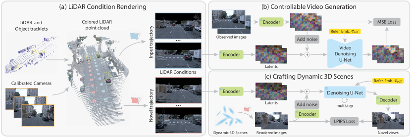
Figure 2: Overview of StreetCrafter. (a) We process the LiDAR using calibrated images and object tracklets to obtain a colorized point cloud, which can be rendered to image space as pixel-level conditions. (b) Given observed images and reference image embedding $\mathbf{c}_{\text{ref}}$, we optimize the video diffusion model conditioned on the LiDAR renderings to perform controllable video generation. (c) Starting from the rendered images and LiDAR conditions under novel trajectory, we use the pretrained controllable video diffusion model to guide the optimization of the dynamic 3DGS representation by generating novel views as extra supervision signals.

2 Related Work

Video Diffusion Models  VDM [20] is the first video diffusion model that applies a diffusion model with a space-time factorized U-Net to a video generation task. Imagen-Video [19] proposes cascaded diffusion models to achieve higher resolution. [3, 15, 56, 59, 78] demonstrate learning VDM in the latent space, enabling high-resolution video generation at low computational cost. [58, 10, 12] learn specific elements and policies from street-view video data, enabling it to generate realistic street-view videos.

To better support downstream applications like reconstruction, some works have proposed camera-controlled video generation methods. [70, 21, 65] propose training-free methods that control the denoising process of an existing diffusion model to achieve controllable video generation. While these methods do not require training or fine-tuning the diffusion model, their performance is limited due to ambiguity during generation. Some recent works finetune the video diffusion model with additional camera parameters as additional input. [55, 26, 34] generate novel views for object-centric scene. Some methods achieve camera control by inject camera parameters into the video diffusion model [66, 60, 61, 1, 54] based on the architecture of U-Net or transformer [40]. Another line of works use geometry foundation models to build explicit representation such as point cloud as guidance to the video diffusion model [29, 71, 36]. However, they mainly focus on static scenes while our method leverages the more accurate LiDAR prior to provide guidance for complex driving scenes.

Street Scene Representation  NeRF [35] and 3DGS [24] have become the leading approaches for modeling autonomous driving scenes. Block-NeRF [50] uses a block-based modeling approach to represent large-scale street scenes. Considering that street scenes typically include moving elements such as vehicles and pedestrians, [53, 68, 5] encode time as an additional input to build 4D representation. [38, 63, 8, 69, 52, 67, 79, 51, 7] decompose the scene into moving objects and static backgrounds, which are reconstructed separately and combined in world space by tracking the moving objects at each time step.

There have been works that try to utilize the LiDAR input [4, 39, 49, 33, 48] to enhance the model’s capability of capturing scene geometry and generalizing to novel viewpoints. However, they mainly deal with static scenes only using supervision from the input trajectory while our model combines the LiDAR with generative prior to generate guidance on novel trajectories for dynamic urban scenes.

Reconstruction with Diffusion Prior  [28, 41] use SDS for lifting 2D generation to 3D, achieving text-based 3D generation. [30, 27, 32] generate multi-view predictions based on a single-view image input using diffusion model, and then use multi-view reconstruction methods to obtain the reconstructed 3D model. [62] enhances sparse-view reconstruction using diffusion prior, and [11] leverages multi-view diffusion to improve multi-view consistency. For scenes with a certain scale, video generation models can more efficiently generate a larger number of novel views with great multi-view consistency compared to image generation models. [29, 71] use DUSt3R [57] to reconstruct the point cloud from sparse viewpoints, leveraging the geometry structure as a condition to guide the video generation model in producing novel-view images, enabling the reconstruction of a static scene with minimal viewpoint input. [6, 31] utilize the degraded rendering results as condition to perform sparse view synthesis with video diffusion models. Recent works [74, 13, 9, 77] enhance street scene reconstruction quality by incorporating diffusion prior to generate additional views, similar to our methods. However, their diffusion models lack precise camera control, which limits the accuracy and visual quality of their reconstruction.

3 Method

Given a recorded autonomous driving scene with calibrated images, LiDAR point clouds, and corresponding object tracklets, our goal is to develop a model capable of synthesizing photorealistic images for novel views. We first give a brief introduction to video diffusion models and 3D Gaussian Splatting in Section 3.1. Then, we introduce our controllable video diffusion model StreetCrafter in Section 3.2. Finally, Section 3.3 discusses how to distill StreetCrafter into a 3D representation for real-time rendering.

3.1 Preliminaries

Video Diffusion Models.

Diffusion models [46, 18] have become a frontline methodology for video generation in recent years. These models learn the underlying data distribution by a forward process and a reverse process. In the forward diffusion process, Gaussian noise $\epsilon\sim\mathcal{N}(0,1)$ is incrementally added to the initial latent $x_{0}\sim p(x)$, resulting in the noisy latent $x_{t}$:

$$x_{t}=\sqrt{\bar{\alpha}_{t}}x_{0}+\sqrt{1-\bar{\alpha}_{t}}\epsilon,$$ (1)

where $t\in\{1,\dots,T\}$ is the diffusion timestep and $\bar{\alpha}_{t}\in(0,1]$ is the noise scheduling parameter. In the reverse diffusion process, the model learns to iteratively denoise the latent to clean data with a trained network $\mathcal{F}_{\theta}(x_{t-1}|x_{t})$. We build our model based on Vista [12], which is a driving world model finetuned from Stable Video Diffusion (SVD) [2] following the continuous-timestep formula [23]. Given conditional input image $c$, the network $\mathcal{F}_{\theta}$ is optimized by the loss function:

$$\mathcal{L}=\mathbb{E}_{x_{0},\epsilon,c,t}\left[\|x_{0}-\mathcal{F}_{\theta}(x_{t},t,c)\|_{2}^{2}\right].$$ (2)

3D Gaussian Splatting.

3DGS  [24] represents the scene using a set of anisotropic Gaussian defined in the 3D world. Each Gaussian $\mathcal{G}$ is assigned with opacity $o\in\mathbb{R}$, spherical harmonics (SH) coefficient $\bm{z}\in\mathbb{R}^{k}$, position vector $\bm{\mu}\in\mathbb{R}^{3}$, rotation quaternion $\bm{q}\in\mathbb{R}^{4}$ and scale factor $\bm{s}\in\mathbb{R}^{3}$. The Gaussian kernel distribution is formulated as:

$$\mathcal{G}(\bm{x})=\exp({-\frac{1}{2}(\bm{x}-\bm{\mu})^{\top}\bm{\Sigma}^{-1}(\bm{x}-\bm{\mu})}),$$ (3)

where $\bm{\Sigma}=\bm{R}\bm{S}\bm{S}^{T}\bm{R}^{T}$, $\bm{S}$ is the scaling matrix determined by $\bm{s}$ and $\bm{R}$ is the rotation matrix determined by $\bm{q}$. Given camera extrinsic $\mathbf{W}$ and intrinsic $\mathbf{K}$, 2D covariance matrix $\bm{\Sigma}^{*}$ in screen space is computed as [80]:

$$\bm{\Sigma}^{*}=\mathbf{J}\mathbf{W}\bm{\Sigma}\mathbf{W}^{T}\mathbf{J}^{T}.$$ (4)

The color $\bm{C}$ of each pixel is rendered by alpha compositing the view-dependent color $\bm{c}$ in depth order:

$$\bm{C}=\sum_{i\in N}\bm{c}_{i}\alpha_{i}\prod_{j=1}^{i-1}(1-\alpha_{j}).$$ (5)

3.2 Controllable Video Generation

In this section, we seek to build a diffusion model that takes a reference image $\mathbf{I}_{\text{ref}}$ and a set of camera trajectories $\{\mathbf{C}_{i}\}_{i=1}^{K}$ to generate the same number of video frames. Previous methods [60, 14] typically rely on camera poses as control signals, which are insufficient for street scenes with complex backgrounds and multiple moving objects. To tackle this problem, we propose a novel controllable video diffusion model StreetCrafter , which leverages the LiDAR input to provide precise control over viewpoint change during the diffusion denoising process.

Building LiDAR condition.

Considering a driving scene with $N$ recorded frames, we first project the LiDAR point cloud onto the calibrated image plane and colorize it by querying the pixel value. Then we utilize the object tracklets to separate the object point cloud from the background, resulting in the background point cloud $\{\mathbf{P}_{i}^{b}\}_{i=1}^{N}$ and object point cloud $\{\mathbf{P}_{i}^{o}\}_{i=1}^{N}$, which are defined in the canonical bounding box coordinate system for each dynamic instance $o$. Given the input camera pose $\mathbf{C}_{i}$ at frame $t_{i}$, we aggregate the LiDAR points within a temporal window of size $l$ to form a unified point cloud $\mathbf{P}$ in the world coordinate system. The object point cloud is warped into the world coordinate system using the object pose $\mathbf{T}_{o}^{t_{i}}$.

Since there still exist numerous missing and occluded regions when treating each point cloud as a pixel in the camera screen, we assign a fixed radius to each LiDAR point in NDC space and perform point rasterization under the camera pose $\mathbf{C}_{i}$ instead of directly projecting $\mathbf{P}$ onto the image plane, yielding the LiDAR condition image $\mathbf{I}^{c}_{i}$ as shown in Figure 2. In this way, we establish a connection between the novel camera trajectories and input calibrated images in a pixel-wise manner by utilizing LiDAR as coarse scene geometry. In comparison with conditional signals, such as camera pose embedding, the LiDAR condition image could provide much stronger guidance as the network only needs to recover clean images from noisy input conditions rather than learning the complicated process of converting camera parameters into video frames.

Training and inference.

To train the model with input images $\{\mathbf{I}_{i}\}_{i=1}^{K}$ and camera trajectory $\{\mathbf{C}_{i}\}_{i=1}^{K}$, we choose the first frame $\mathbf{I}_{0}$ as reference image $\mathbf{I}_{\text{ref}}$ and obtain the corresponding LiDAR conditions $\{\mathbf{I}^{c}_{i}\}_{i=1}^{K}$, as shown in Figure 2. The inputs and LiDAR conditions are further encoded into latent space as $\{\mathbf{z}_{i}\}_{i=1}^{K}$ and $\{\mathbf{z}^{c}_{i}\}_{i=1}^{K}$ with a pre-trained VAE encoder. We then inject $\mathbf{z}^{c}_{i}$ into the first layer of the U-Net architecture by adding a trainable zero convolutional layer [75] $\Theta_{z}$ to $\mathcal{F}_{\theta}$ and perform element-wise addition:

$$\hat{\mathbf{z}}_{i,t}=\mathbf{z}_{i,t}+\mathcal{Z}(\mathbf{z}^{c}_{i}\,;\,\Theta_{z}),$$ (6)

where $\mathcal{Z}(\cdot\,;\,\Theta_{z})$ indicates the zero convolutional layer and $\mathbf{z}_{i,t}$ is the noisy latent from $\mathbf{z}_{i}$ and diffusion timestep $t$ using Eq. 1. We find that this minor modification could provide sufficient guidance without introducing additional computation costs. The video denoising U-Net $\mathcal{F}_{\theta}$ is optimized by minimizing the following loss objective:

$$\mathcal{L}=\mathbb{E}_{\mathbf{z}_{i},\epsilon,\mathbf{c}_{\text{ref}},,c_{\text{p},t}}\left[\|\mathbf{z}_{i}-\mathcal{F}_{\theta}(\hat{\mathbf{z}}_{i,t},t,\mathbf{c}_{\text{ref}},\mathbf{c}_{\text{p}})\|_{2}^{2}\right],$$ (7)

where $\mathbf{c}_{\text{ref}}$ and $\mathbf{c}_{\text{p}}$ refer to the reference image CLIP embedding [42] and LiDAR conditions respectively.

During inference with novel camera trajectory $\{\hat{\mathbf{C}}_{i}\}_{i=1}^{K}$ as input, we select the input camera closest to $\hat{\mathbf{C}}_{1}$ as reference image $\mathbf{I}_{\text{ref}}$ and render the novel view LiDAR conditions denoted as $\{\hat{\mathbf{I}}^{c}_{i}\}_{i=1}^{K}$. Starting from sampled noise $\epsilon\sim\mathcal{N}(0,I)$, we iteratively denoise the noisy latent $\hat{\mathbf{z}}_{i}$ with the trained denoising network $\mathcal{F}_{\theta}$ conditioned on $\{\hat{\mathbf{I}}^{c}_{i}\}_{i=1}^{K}$ and $\mathbf{I}_{\text{ref}}$ into clean latents, which is further decoded into novel view images $\{\hat{\mathbf{I}}_{i}\}_{i=1}^{K}$ with a pre-trained VAE decoder.

3.3 Crafting Dynamic 3D Scenes

In this section, our goal is to distill the generative prior of the controllable video diffusion model into a more consistent 3DGS [24] representation for real-time rendering. The main drawback of 3DGS is that it cannot generalize well to novel viewpoints away from input cameras, which is a common problem for reconstruction-based methods. To address this issue, we propose a novel framework that leverages our video diffusion model to apply constraints to 3DGS along novel trajectories during optimization.

Scene representation.

To model dynamic urban scenes with 3DGS, we follow existing approaches [67, 7] and use a distinct set of Gaussian parameters to model the background and each foreground moving object. The object Gaussians $\mathcal{G}_{v}$ is defined in the canonical coordinate system determined by the object tracklets. Given the SE(3) pose $\bm{T}_{v}^{t}=(\bm{R}_{v}^{t},\bm{t}_{v}^{t})$ at timestamp $t$, $\mathcal{G}_{v}$ can be mapped into the world coordinate system for global rendering as:

$$\hat{\bm{\mu}}_{v}=\bm{R}_{v}^{t}\bm{\mu}_{v}+\bm{t}_{v}^{t},\quad\hat{\bm{R}}_{v}=\bm{R}_{v}^{t}\bm{R}_{v},$$ (8)

where $\bm{\mu}_{v},\bm{R}_{v}$ and $\hat{\bm{\mu}}_{v},\hat{\bm{R}}_{v}$ denotes the position and rotation of $\mathcal{G}_{v}$ in local and world coordinate system, respectively. The distant region of the scene is modeled by a high-resolution cubemap, which is combined with the rendered color $\bm{C}_{\mathcal{G}}$ from Eq. 5 using rendered opacity $\bm{O}_{\mathcal{G}}$.

Novel view generation.

To better align the generated video frames from the diffusion model with the 3DGS scene representation, we generate samples from the noisy rendered latent instead of pure noise inspired by previous works [62, 41]. We find this can help maintain the overall scene structure and accelerate the training process due to fewer denoising steps. To be specific, we render images $\{{\mathbf{I}}_{i}^{r}\}_{i=1}^{K}$ from novel views $\{\hat{\mathbf{C}}_{i}\}_{i=1}^{K}$, which are encoded and perturbed to noisy latents $\{\mathbf{z}_{i,t}^{r}\}_{i=1}^{K}$ given diffusion timestep $t$ derived from noise scale $s$. Then we generate samples from the denoising U-Net by running the DDIM sampling [45]. The samples are further decoded to novel view images $\{\hat{\mathbf{I}}_{i}\}_{i=1}^{K}$ for supervision. Based on the following generation process, we employ a progressive optimization strategy by gradually reducing the noise scale $s$. This helps the model learn to remove artifacts by relying more on the diffusion prior in the early training stage and progressively focusing on refining details as the training advances.

Loss function.

We construct our training set by combining input views with novel views generated by the video diffusion model. In each training iteration, we randomly sample a camera $\mathbf{C}$ with the ratio of selecting a novel view camera set to $p$. The Gaussian scene representation $\mathcal{G}$ is optimized using the following loss function:

$$\mathcal{L}_{\text{input}}=\lambda_{1}\mathcal{L}_{1}+ \lambda_{\text{ssim}}\mathcal{L}_{\text{ssim}}+\lambda_{\text{lpips}}\mathcal{L}_{\text{lpips}}+\mathcal{L}_{\text{g}},$$ (9)

$$\mathcal{L}_{\text{novel}} =\lambda_{\text{novel}}\mathcal{L}_{\text{lpips}},$$

where $\mathcal{L}_{1}$, $\mathcal{L}_{\text{ssim}}$, and $\mathcal{L}_{\text{lpips}}$ denote the $L_{1}$, SSIM, and LPIPS losses, respectively. we select either $\mathcal{L}_{\text{input}}$ or $\mathcal{L}_{\text{novel}}$ as the loss function depending on whether $C$ is a novel view. In comparison with the original loss function of 3DGS, we additionally introduce the LPIPS [76] loss between the rendered and generated image of novel view as it emphasizes high-level semantic similarity rather than photometric consistency. We also add an extra loss $\mathcal{L}_{g}$ for all input views, which includes LiDAR depth loss $\mathcal{L}_{\text{depth}}$, sky mask loss $\mathcal{L}_{\text{sky}}$ and moving objects regularization loss $\mathcal{L}_{\text{reg}}$ to further enhance the scene geometry. Please refer to the supplementary material for more details on each loss term.

4 Implementation Details

We initialize StreetCrafter from the pretrained checkpoint of Vista [12]. We first train all the parameters of the video denoising U-Net at the resolution of 320 $\times$ 576 with batch size of 16 and learning rate of $5e^{-5}$ for 30000 iterations. Then we fix the temporal layers and finetune the spatial layers of U-Net at the resolution of 576 $\times$ 1024 with batch size of 8 and learning rate of $1e^{-5}$ for another 3000 iterations. During training, we randomly drop the reference image and LiDAR conditions with a probability of 15% independently. It takes 2 days to train the model on 8 NVIDIA A800 80GB GPUs using Adam [25] optimizer. During inference, we set the sampling steps to 50 and classifier-free guidance (CFG) [17] scale to 2.5 and generate videos of length $n=25$ at the resolution of $576\times 1024$. For novel trajectories longer than $n$, we iteratively sample $n$-length video frames with an overlapping frame length of 5 to construct the full-length video. The temporal window size $l$ is set to cover the LiDAR point cloud from adjacent $\pm 1s$ frames.

During the distillation process from StreetCrafter to 3DGS, we follow the setting of Street Gaussians [67] and train the model for 30000 iterations. The novel trajectory is built by shifting the input cameras lateral to the heading direction of the ego vehicle for 3 meters across the sequence and we sample the novel view cameras with the ratio $p$ set to 0.4. The coefficients $\lambda_{1}$, $\lambda_{\text{ssim}}$, $\lambda_{\text{lpips}}$ and $\lambda_{\text{novel}}$ are set to 0.2, 0.8, 0.5 and 0.1, respectively. The training takes about 1.5 hours on one A800 GPU.

5 Experiments

5.1 Experiments Setup

We evaluate the performance of StreetCrafter and the crafted dynamic 3DGS representation which we referr to as Ours-V and Ours-G respectively on the task of novel view synthesis. For Ours-V, we crop and resize the input image to 576 $\times$ 1024 to match the output resolution of video diffusion model during evaluation. Datasets.  We conduct experiments on Waymo Open Dataset [47] and PandaSet [64], using their 10Hz front camera and synchronized LiDAR. We select 15 sequences of approximately 100 frames from the validation set of Waymo and 5 sequences of 80 frames from PandaSet to test the novel view synthesis results. We uniformly sample half of the images in each sequence as the testing frames and use the remaining for training. Input image resolution is set to $1066\times 1600$ and $900\times 1600$ for Waymo and PandaSet, respectively. The training set of Waymo and the remaining PandaSet sequences are used to train StreetCrafter, resulting in a total of approximately 35,000 training samples. More details can be found in the supplementary.

Baselines.  We compare our method with 3DGS [24], Street Gaussians [67], EmerNeRF [68], UniSim [69] and NeuRAD [52]. Street Gaussians [67] models the background and each moving object using separate Gaussian models. EmerNeRF [68] stratifies scenes into static and dynamic fields, each modeled with a hash grid [37]. UniSim [69] and NeuRAD [52] utilize neural feature grids to model dynamic driving scenes with CNN renderer to enhance the ability of view extrapolation. We enhance 3DGS by incorporating LiDAR depth supervision and LiDAR point cloud initialization. For the rest of the methods, we evaluated the results based on their official implementations.

Figure 3: Qualitative comparisons on the Waymo [47] dataset. The camera is laterally shifted for 3 meters to left or right. Input view refers to the closest training camera. Ours-G denotes the dynamic 3DGS distilled from StreetCrafter and Ours-V denotes StreetCrafter.

Figure 4: Qualitative comparisons on the PandaSet [64] dataset. The camera is laterally shifted for 3 meters to left or right.

Methods	Interpolation		Lane Shift		FPS
	PSNR$\uparrow$	LPIPS$\downarrow$	FID$\downarrow$ @ 2m	FID$\downarrow$ @ 3m
Ours-V	27.19	0.087	62.43	73.49	0.16
3DGS [24]	28.85	0.148	100.50	122.52	213.37
EmerNeRF [68]	26.09	0.199	89.98	110.78	0.20
Street Gaussians [67]	30.95	0.130	71.42	93.38	92.16
Ours-G	30.05	0.054	58.17	71.40	113.16

Table 1: Quantitative results on the Waymo [47] dataset. The rendering image resolution is 1066 $\times$ 1600. Ours-G denotes the dynamic 3DGS distilled from StreetCrafter and Ours-V denotes StreetCrafter tested under the resolution of 576 $\times$ 1024.

Methods	Interpolation		Lane Shift		FPS
	PSNR$\uparrow$	LPIPS$\downarrow$	FID$\downarrow$ @ 2m	FID$\downarrow$ @ 3m
Ours-V	26.10	0.090	69.68	81.99	0.19
3DGS [24]	26.11	0.135	127.74	143.94	86.98
UniSim [69]	25.62	0.121	75.26	92.65	6.43
NeuRAD [52]	27.00	0.098	64.65	86.44	6.01
Street Gaussians [67]	27.54	0.109	69.87	90.41	88.47
Ours-G	26.68	0.062	62.15	78.88	80.56

Table 2: Quantitative results on the PandaSet [64] dataset. The rendering image resolution is 900 $\times$ 1600.

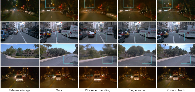
Figure 5: Visual ablation results on the design choice of StreetCrafter. The results indicate that our LiDAR condition can provide more accurate control for street view synthesis even when the viewpoint deviates greatly from the reference image.

5.2 Comparisons Results

Tables 1, 2 present the comparison results of our method with baseline methods [24, 67, 69, 52, 68] in terms of rendering quality and rendering speed. We assess the rendering quality under the setting of view interpolation and extrapolation. We adopt PSNR and LPIPS [76] as evaluation metrics for view interpolation and report FID [16] under the setting of lane shift for view extrapolation since no ground truth image is available. Our method achieves state-of-the-art performance in extrapolation scenarios while maintaining comparable results for interpolation.

Figures 3, 4 display the qualitative differences. Baseline methods tend to generate blurry results with artifacts, particularly in challenging and under-observed regions such as lanes and moving vehicles, while both Ours-G and Ours-V can both generate high-fidelity novel views, thanks to the LiDAR conditions, diffusion prior, and distillation process. Moreover, Ours-G can achieve rendering speed similar to Street Gaussians [67] but demonstrates superior large-view generalization capability as shown in the FID metric.

5.3 Ablation Studies

We first analyze the design choice of StreetCrafter presented in Section 3.2 with several variants on two types of settings from the validation set of Waymo [47] dataset as shown in Table 3. For the random set, we randomly select 40 video clips from 10 uniformly sampled Waymo sequences. We further specifically choose 10 video clips from which include complex behaviors such as turnings and lane changes to form the hard set. All the videos have a frame length of 25 with the first frame selected as the reference image and all the variants are trained under the same setting as our model. Finally, we ablate on several optimization strategies during the distillation process presented in Section 3.3.

Methods	Random set			Hard set
	PSNR $\uparrow$	LPIPS $\downarrow$	FID $\downarrow$	PSNR $\uparrow$	LPIPS $\downarrow$	FID $\downarrow$
(1) Plücker embedding	22.88	0.233	92.75	17.59	0.421	149.35
(2) Pose + 3D box	24.54	0.201	90.36	18.81	0.395	159.86
(3) Single frame LiDAR	25.57	0.156	73.25	20.62	0.272	106.01
(4) Projected LiDAR	26.15	0.135	66.29	21.57	0.246	100.51
(5) Ours	27.00	0.121	55.53	22.23	0.218	77.03

Table 3: Ablation study on the design choice of StreetCrafter. Metrics are averaged over all sampled video clips and our complete model achieves the best performance.

Figure 6: Visual ablation results on the distillation of StreetCrafter. The camera is laterally shifted for 3 meters to the left. Our framework refines the texture details of nearby regions while maintaining the 3D structure in areas without LiDAR conditions.

Our model with camera pose condition.  We compare StreetCrafter with two variants conditioned on camera pose as shown in Rows 1-2 of Table 3. We first replace the LiDAR condition with Plücker embeddings [44] of camera rays as the pose representation. Although ray embedding serves as a pixel-level condition, it fails to build relationships between the camera pose and the scene geometry. As shown in Figure 5, the model lacks precise control and results in blurriness as the viewpoint diverges from the reference image. We then treat the camera parameter as a vector and inject it into the temporal attention layer of the denoising U-Net [60]. To better model object motions, we replace our LiDAR condition with projected object 3D bounding box similar to recent world models [58, 77]. As shown in Table 5, the experimental results indicate that it lacks controllability due to the complexity of the driving scene.

Methods	Interpolation		Lane Shift
	PSNR$\uparrow$	LPIPS$\downarrow$	FID$\downarrow$ @ 2m	FID$\downarrow$ @ 3m
(1) Ours w/o LPIPS loss	30.80	0.108	69.16	79.63
(2) Ours w/o novel weight	29.38	0.054	71.97	82.11
(3) Ours w/o noise scale	30.86	0.044	65.80	77.59
(4) Ours	30.88	0.043	64.70	73.45

Table 4: Ablation study on the distillation of StreetCrafter. Metrics are averaged over the selected sequences and our complete model achieves the best performance.

The influence of rendering aggregated LiDAR.  We compare StreetCrafter with two variants conditioned on LiDAR shown in Rows 3-4 of Table 3. We first change the aggregated LiDAR point cloud to single-frame LiDAR input. As shown in Figure 5, the generated video lacks fidelity in representing scene texture details, such as the icons on the road since the single-frame LiDAR is extremely sparse even rendered with radius in screen space. We then create another variant that directly projects the aggregated LiDAR point cloud without assigning each point a fixed radius in the image screen space. The results in Table 3 indicate that our model performs better since the projected point cloud has difficulty handling occlusion relationships .

Analysis of the distillation process.  We carry out ablation studies on two sequences from the Waymo [47] dataset to analyze our StreetCrafter distillation framework in Table 4 and Figure 6. (1) We set $\lambda_{\text{lpips}}$ to 0 and change $\mathcal{L}_{\text{novel}}$ to L1 loss. The result in Figure 6 indicates that LPIPS loss helps recover sharp details under a novel viewpoint. (2) We remove the novel weight by setting $\lambda_{\text{novel}}$ as 1.0. There is a significant drop in all the metrics and many artifacts appear on the moving object as shown in Figure 6, which highlights the importance of treating input views and novel views independently. (3) We set the noise scale $s$ to 1 throughout the training so that the model always starts from a pure noise. Artifacts appear in areas where LiDAR conditions are lacking, such as the road signs on traffic lights.

5.4 Scene Editing

StreetCrafter supports various editing operations for moving objects. We can achieve object translation (Figure 7 (a)), replacement (Figure 7 (b)) and removal (Figure 7 (c)) by adjusting the attributes of the object bounding boxes during multi-frame point cloud aggregation to provide modified LiDAR conditions for the video diffusion model. In contrast to previous reconstruction methods [52, 69, 67], which model each object separately, StreetCrafter can perform editing operations without per-scene optimization.

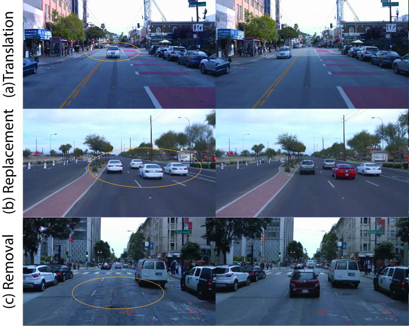
Figure 7: Editing results on the Waymo [47] dataset. StreetCrafter supports various editing operations, including translation, replacement, and removal. Images in the right and left columns represent the results before and after editing, respectively.

6 Conclusion

This paper introduced StreetCrafter, a controllable video diffusion model for street view synthesis. The key insight is to leverage sparse yet geometrically accurate LiDAR to provide pixel-level conditions for precise camera control, enabling the model to generate consistent video frames aligned with the camera inputs. By further distilling StreetCrafter into a 3DGS [24] model, we enable real-time view synthesis in challenging scenarios, such as lane shift. Moreover, scene editing is possible by providing modified LiDAR conditions to the video diffusion model. Detailed ablation and comparisons are conducted on several datasets, demonstrating the effectiveness of the proposed methods.

This work also has some known limitations. First, collecting the necessary LiDAR data and object tracklets for training StreetCrafter is costly due to the extensive data collection and processing requirements. Second, the inference speed of StreetCrafter remains significantly short of real-time due to the architecture of video denoising U-Net. Future work could consider employing a more advanced model for real-time inference.

Appendix

Appendix A More Implementation Details

A.1 StreetCrafter Training Details

We construct the training video clips using the front camera and LiDAR sensor of Waymo Open  [47] and PandaSet [64] datasets, with the start frame of each video clip selected at the interval of 0.5 second (5 frames for both dataset). We set the radius of each LiDAR point cloud in NDC space to 0.01 and crop the upper part of LiDAR condition maps to match the input resolution of the diffusion model during both training and inference.

For the adaptation from the pretrained model of Vista [12], we ignore the action control layer injected via cross-attention and mark the first element of the frame-wise mask to 1 and the rest to 0. We incorporate the LoRA [22] adapters introduced during the learning of action controllability as it contributes to the enhancement of visual quality [12]. More details can be found in the original paper.

During the low-resolution training stage, we sample exclusively from Waymo dataset. During the high-resolution training stage, we sample from a hybrid dataset, combining Waymo Open and PandaSet datasets with sampling probabilities of 0.9 and 0.1, respectively.

A.2 StreetCrafter Distillation Details

Loss function.

We jointly optimize the gaussian parameters of background and foreground moving objects, texel of the high-resolution sky cubemap and noisy object tracklets following Street Gaussians [67]. The extra loss $\mathcal{L}_{\text{g}}$ for input view camera is defined as:

$$\mathcal{L}_{\text{g}}=\lambda_{\text{depth}}\mathcal{L}_{\text{depth}}+\lambda_{\text{sky}}\mathcal{L}_{\text{sky}}+\lambda_{\text{reg}}\mathcal{L}_{\text{reg}}.$$ (10)

For $\mathcal{L}_{\text{depth}}$, we apply the $\mathcal{L}_{1}$ loss between rendered depth $\mathbf{D}$ and the LiDAR measurement’s depth $\mathbf{D}^{\text{lidar}}$ where we optimize 95% of the pixels with smallest depth error:

$$\mathcal{L}_{\text{depth}}=\sum||\mathbf{D}-\mathbf{D}^{\text{lidar}}||_{1}.$$ (11)

For $\mathcal{L}_{\text{sky}}$, we apply the binary cross entropy loss between rendered opacity $\mathbf{O}_{g}$ and predicted sky mask $\mathbf{M}_{\text{sky}}$ generated by Grounded SAM [43]:

$$\mathcal{L}_{\text{sky}}=-\sum((1-\mathbf{M}_{\text{sky}})\text{log}\mathbf{O}_{g}+\mathbf{M}_{\text{sky}}\text{log}(1-\mathbf{O}_{g})).$$ (12)

For $\mathcal{L}_{\text{reg}}$, the regularization term in our loss function is defined as an entropy loss on the accumulated alpha values of decomposed foreground objects $\mathbf{O}_{\text{obj}}$:

$$\mathcal{L}_{\text{reg}}=-\sum(\mathbf{O}_{\text{obj}}\text{log}\mathbf{O}_{\text{obj}}+(1-\mathbf{O}_{\text{obj}})\text{log}(1-\mathbf{O}_{\text{obj}})).$$ (13)

The coefficients $\lambda_{\text{depth}}$, $\lambda_{\text{sky}}$ and $\lambda_{\text{reg}}$ in Equation 10 are set to 0.01, 0.05 and 0.1, respectively. For the loss function of novel view camera, we crop the upper part of the rendering image and resize to $576\times 1024$ to compute the LPIPS [76] loss with novel view image generated by StreetCrafter .

Point cloud initialization.

We initialize the background gaussian model as the combination of LiDAR and SfM point cloud following. The object gaussian model is initialized with aggregated LiDAR points obtained from object tracklets or random sampling. The colors of LiDAR points are assigned by projecting them onto the image plane.

Optimization.

We adopt the densification strategy introduced in [73] to prevent suboptimal solutions by accumulating the norms of view-space position gradients. The densification threshold is set to 0.0006. We disable the pruning of big gaussians in world space since this hinders the gaussian model to represent distant regions and the LiDAR points have provided a good initialization to prevent the model from falling into local optima. We finally introduce the 2D Mip filter to enable anti-aliased rendering inspired by [72].

We sample StreetCrafter every 5000 iterations from iteration 7000 to 22000 and linearly reduce the noise scale $s$ from 0.7 to 0.3. We use the annotated object tracklets provided by the datasets, with the learning rates for the translation vector and rotation matrix initialized at $5e^{-4}$ and $1e^{-5}$, respectively, decaying exponentially to $1e^{-5}$ and $5e^{-6}$. For the remaining parameters, we use the default values from the official implementation of Street Gaussians [67].

A.3 Evaluation Details

Interpolation of StreetCrafter.

For the interpolation setting of Ours-V in the main paper, we incorporate training images along the input trajectory in addition to the reference image and LiDAR conditions. During each denoising step, we replace the prediction of $\mathcal{F}_{\theta}$ at training frame with the clean latent of training images. This could lead to improvement in the interpolation quality, with PSNR increasing from 23.66 to 27.19 and LPIPS decreasing from 0.098 to 0.087 on Waymo Open Dataset [47].

Baselines.

We use the same object tracklets as our method for all the baselines requiring 3D bounding box as input [67, 52, 69]. We use the same rendering kernel and optimization strategy as our method for all the baselines using 3DGS as the scene representation [24, 67].

Appendix B Additional Experiments

B.1 More Editing Results

We provide more visual results of scene editing in Figure 8 including object translation, replacement and removal.

B.2 More Comparisons

We provide more qualitative comparisons on Waymo [47] dataset under the setting of lane change in Figure 10.

B.3 Interpolation Results

Figures 11, 12 display the view interpolation results on Waymo Open [47] and PandaSet [64] datasets. Our method achieves comparable rendering quality to the baselines while delivering significantly better results for view extrapolation.

B.4 More Ablations

Analysis of LiDAR conditions

We present more visual comparisons of the design choice of StreetCrafter in Figure 9. The generated frames under the guidance of camera parameter as vector are blurry when the target viewpoint move away from the reference image. Although the 3D bounding box can provide priors regrading object motions, it still fails to align well with the target image as shown in the first row of Figure 9. The results under the condition of projected multi-frame LiDAR can preserve the scene structure but still lack details in regions with rich texture.

Analysis of the novel view sampling ratio

We conduct experiment on one Waymo sequence to analyze the influence of novel view sampling ratio $p$. The results in Table 5 indicates that $p=0.4$ yields the overall best result.

Methods	Interpolation		Lane Shift
	PSNR$\uparrow$	LPIPS$\downarrow$	FID$\downarrow$ @ 2m	FID$\downarrow$ @ 3m
(1) $p=0.8$	28.76	0.059	72.76	84.78
(2) $p=0.6$	29.61	0.049	68.33	81.26
(3) $p=0.4$	30.42	0.041	67.54	79.19
(4) $p=0.2$	30.29	0.041	67.09	81.26

Table 5: Ablations on the novel view sampling ratio $p$.

Figure 8: More editing results on the Waymo [47] dataset. Images in the right and left columns represent the results before and after editing, respectively.

Analysis of the noise scale

We conduct experiment on one Waymo sequence to analyze the influence of noise scale $s$.s We have demonstrated in the main paper that adding noise to the render latents leads to better scene consistency than starting from gaussian noise. Since the added noise would have little influence when $s$ is less than 0.3 according to the sampling scheme of Vista [23], we set $s_{\text{min}}$ to 0.3 and ablate on the value of $s_{\text{max}}$. The results in Table 6 indicates that reducing $s$ from 0.7 to 0.3 maintains a balance between sampling steps and rendering quality.

Methods	Interpolation		Lane Shift
	PSNR$\uparrow$	LPIPS$\downarrow$	FID$\downarrow$ @ 2m	FID$\downarrow$ @ 3m
(1) $s_{\text{max}}=1.0,s_{\text{min}}=0.3$	30.08	0.044	69.66	79.87
(2) $s_{\text{max}}=0.7,s_{\text{min}}=0.3$	30.42	0.041	67.54	79.19
(3) $s_{\text{max}}=0.5,s_{\text{min}}=0.3$	30.46	0.042	68.68	81.23

Table 6: Ablations on the noise scale $s$.

B.5 Deformable Objects

We show the generated videos of StreetCrafter under scene with multiple deformable objects such as pedestrians in Figure 13. Although multi-frame LiDAR conditions are not ideal for deformable objects, our model can generate plausible results with the generative prior of diffusion model.

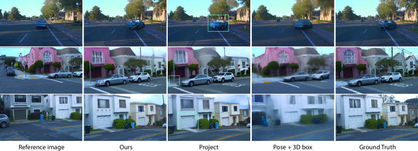
Figure 9: Visual ablation results on the design choice of StreetCrafter.

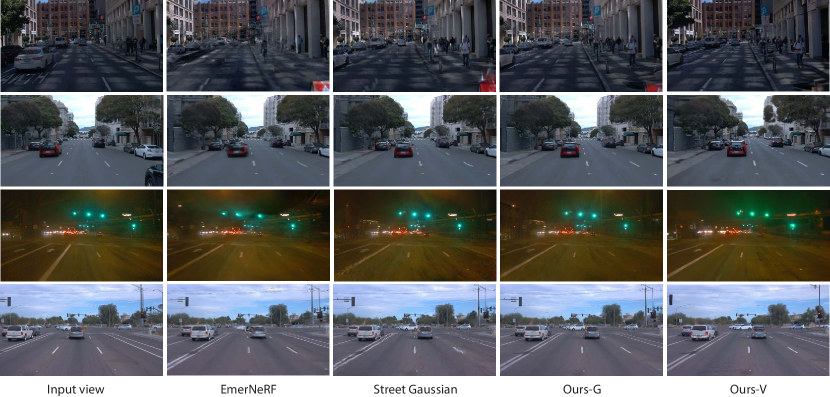
Figure 10: Qualitative comparisons on the Waymo [47] dataset. The camera is laterally shifted for 2 meters to left or right. Input view refers to the closest training camera.

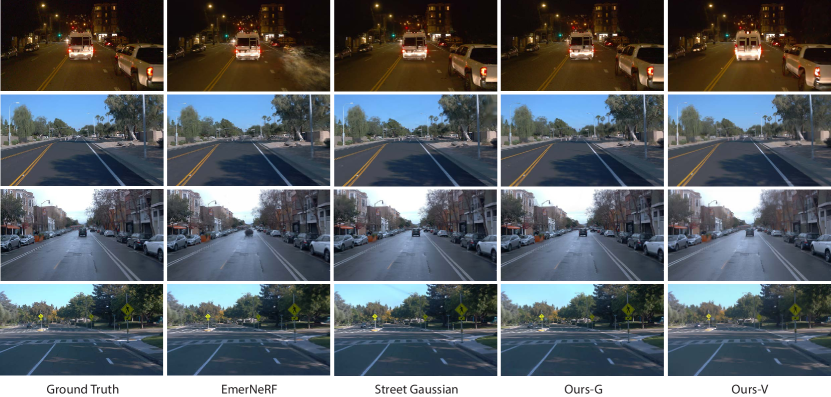
Figure 11: Qualitative comparisons of view interpolation on the Waymo [47] dataset.

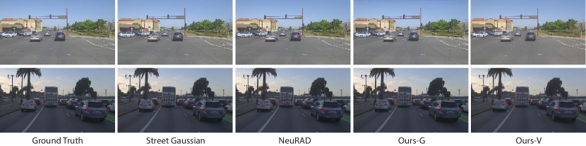
Figure 12: Qualitative comparisons of view interpolation on the PandaSet [64] dataset.

Figure 13: Visual results of StreetCrafter for scene with deformable objects.

References

- Bahmani et al. [2024] Sherwin Bahmani, Ivan Skorokhodov, Aliaksandr Siarohin, Willi Menapace, Guocheng Qian, Michael Vasilkovsky, Hsin-Ying Lee, Chaoyang Wang, Jiaxu Zou, Andrea Tagliasacchi, David B. Lindell, and Sergey Tulyakov. Vd3d: Taming large video diffusion transformers for 3d camera control. arXiv preprint arXiv:2407.12781, 2024.
- Blattmann et al. [2023a] Andreas Blattmann, Tim Dockhorn, Sumith Kulal, Daniel Mendelevitch, Maciej Kilian, Dominik Lorenz, Yam Levi, Zion English, Vikram Voleti, Adam Letts, Varun Jampani, and Robin Rombach. Stable video diffusion: Scaling latent video diffusion models to large datasets, 2023a.
- Blattmann et al. [2023b] Andreas Blattmann, Robin Rombach, Huan Ling, Tim Dockhorn, Seung Wook Kim, Sanja Fidler, and Karsten Kreis. Align your latents: High-resolution video synthesis with latent diffusion models. In CVPR, 2023b.
- Chang et al. [2023] MingFang Chang, Akash Sharma, Michael Kaess, and Simon Lucey. Neural radiance field with lidar maps. In ICCV, 2023.
- Chen et al. [2023] Yurui Chen, Chun Gu, Junzhe Jiang, Xiatian Zhu, and Li Zhang. Periodic vibration gaussian: Dynamic urban scene reconstruction and real-time rendering. arXiv:2311.18561, 2023.
- Chen et al. [2024a] Yuedong Chen, Chuanxia Zheng, Haofei Xu, Bohan Zhuang, Andrea Vedaldi, Tat-Jen Cham, and Jianfei Cai. Mvsplat360: Feed-forward 360 scene synthesis from sparse views. In NeurIPS, 2024a.
- Chen et al. [2024b] Ziyu Chen, Jiawei Yang, Jiahui Huang, Riccardo de Lutio, Janick Martinez Esturo, Boris Ivanovic, Or Litany, Zan Gojcic, Sanja Fidler, Marco Pavone, Li Song, and Yue Wang. Omnire: Omni urban scene reconstruction. arXiv preprint arXiv:2408.16760, 2024b.
- Fischer et al. [2024] Tobias Fischer, Jonas Kulhanek, Samuel Rota Bulò, Lorenzo Porzi, Marc Pollefeys, and Peter Kontschieder. Dynamic 3d gaussian fields for urban areas. In NeurIPS, 2024.
- Gao et al. [2024a] Ruiyuan Gao, Kai Chen, Zhihao Li, Lanqing Hong, Zhenguo Li, and Qiang Xu. Magicdrive3d: Controllable 3d generation for any-view rendering in street scenes. arXiv preprint arXiv:2405.14475, 2024a.
- Gao et al. [2024b] Ruiyuan Gao, Kai Chen, Enze Xie, Lanqing Hong, Zhenguo Li, Dit-Yan Yeung, and Qiang Xu. MagicDrive: Street view generation with diverse 3d geometry control. In ICLR, 2024b.
- Gao* et al. [2024] Ruiqi Gao*, Aleksander Holynski*, Philipp Henzler, Arthur Brussee, Ricardo Martin-Brualla, Pratul P. Srinivasan, Jonathan T. Barron, and Ben Poole*. Cat3d: Create anything in 3d with multi-view diffusion models. In NeurIPS, 2024.
- Gao et al. [2024] Shenyuan Gao, Jiazhi Yang, Li Chen, Kashyap Chitta, Yihang Qiu, Andreas Geiger, Jun Zhang, and Hongyang Li. Vista: A generalizable driving world model with high fidelity and versatile controllability. In NeurIPS, 2024.
- Han et al. [2024] Huasong Han, Kaixuan Zhou, Xiaoxiao Long, Yusen Wang, and Chunxia Xiao. Ggs: Generalizable gaussian splatting for lane switching in autonomous driving. arXiv preprint arXiv:2409.02382, 2024.
- He et al. [2024] Hao He, Yinghao Xu, Yuwei Guo, Gordon Wetzstein, Bo Dai, Hongsheng Li, and Ceyuan Yang. Cameractrl: Enabling camera control for text-to-video generation. arXiv preprint arXiv:2404.02101, 2024.
- He et al. [2022] Yingqing He, Tianyu Yang, Yong Zhang, Ying Shan, and Qifeng Chen. Latent video diffusion models for high-fidelity video generation with arbitrary lengths. arXiv preprint arXiv:2211.13221, 2(3):4, 2022.
- Heusel et al. [2017] Martin Heusel, Hubert Ramsauer, Thomas Unterthiner, Bernhard Nessler, and Sepp Hochreiter. Gans trained by a two time-scale update rule converge to a local nash equilibrium. In NeurIPS, 2017.
- Ho and Salimans [2021] Jonathan Ho and Tim Salimans. Classifier-free diffusion guidance. In NeurIPS, 2021.
- Ho et al. [2020] Jonathan Ho, Ajay Jain, and Pieter Abbeel. Denoising diffusion probabilistic models. In NeurIPS, 2020.
- Ho et al. [2022a] Jonathan Ho, William Chan, Chitwan Saharia, Jay Whang, Ruiqi Gao, Alexey Gritsenko, Diederik P Kingma, Ben Poole, Mohammad Norouzi, David J Fleet, et al. Imagen video: High definition video generation with diffusion models. arXiv preprint arXiv:2210.02303, 2022a.
- Ho et al. [2022b] Jonathan Ho, Tim Salimans, Alexey Gritsenko, William Chan, Mohammad Norouzi, and David J Fleet. Video diffusion models. In NeurIPS, 2022b.
- Hou et al. [2024] Chen Hou, Guoqiang Wei, Yan Zeng, and Zhibo Chen. Training-free camera control for video generation. arXiv preprint arXiv:2406.10126, 2024.
- Hu et al. [2022] Edward J Hu, Yelong Shen, Phillip Wallis, Zeyuan Allen-Zhu, Yuanzhi Li, Shean Wang, Lu Wang, and Weizhu Chen. LoRA: Low-rank adaptation of large language models. In ICLR, 2022.
- Karras et al. [2022] Tero Karras, Miika Aittala, Timo Aila, and Samuli Laine. Elucidating the design space of diffusion-based generative models. In NeurIPS, 2022.
- Kerbl et al. [2023] Bernhard Kerbl, Georgios Kopanas, Thomas Leimkühler, and George Drettakis. 3d gaussian splatting for real-time radiance field rendering. ACM Transactions on Graphics, 42(4), 2023.
- Kingma and Ba [2014] Diederik P Kingma and Jimmy Ba. Adam: A method for stochastic optimization. arXiv preprint arXiv:1412.6980, 2014.
- Kwak et al. [2024] Jeong-gi Kwak, Erqun Dong, Yuhe Jin, Hanseok Ko, Shweta Mahajan, and Kwang Moo Yi. Vivid-1-to-3: Novel view synthesis with video diffusion models. In CVPR, 2024.
- Li et al. [2024] Jiahao Li, Hao Tan, Kai Zhang, Zexiang Xu, Fujun Luan, Yinghao Xu, Yicong Hong, Kalyan Sunkavalli, Greg Shakhnarovich, and Sai Bi. Instant3d: Fast text-to-3d with sparse-view generation and large reconstruction model. In ICLR, 2024.
- Lin et al. [2023] Chen-Hsuan Lin, Jun Gao, Luming Tang, Towaki Takikawa, Xiaohui Zeng, Xun Huang, Karsten Kreis, Sanja Fidler, Ming-Yu Liu, and Tsung-Yi Lin. Magic3d: High-resolution text-to-3d content creation. In CVPR, 2023.
- Liu et al. [2024a] Fangfu Liu, Wenqiang Sun, Hanyang Wang, Yikai Wang, Haowen Sun, Junliang Ye, Jun Zhang, and Yueqi Duan. Reconx: Reconstruct any scene from sparse views with video diffusion model. arXiv preprint arXiv:2408.16767, 2024a.
- Liu et al. [2024b] Minghua Liu, Chao Xu, Haian Jin, Linghao Chen, Mukund Varma T, Zexiang Xu, and Hao Su. One-2-3-45: Any single image to 3d mesh in 45 seconds without per-shape optimization. In NeurIPS, 2024b.
- Liu et al. [2024c] Xi Liu, Chaoyi Zhou, and Siyu Huang. 3dgs-enhancer: Enhancing unbounded 3d gaussian splatting with view-consistent 2d diffusion priors. In NeurIPS, 2024c.
- Long et al. [2024] Xiaoxiao Long, Yuan-Chen Guo, Cheng Lin, Yuan Liu, Zhiyang Dou, Lingjie Liu, Yuexin Ma, Song-Hai Zhang, Marc Habermann, Christian Theobalt, et al. Wonder3d: Single image to 3d using cross-domain diffusion. In CVPR, 2024.
- Lu et al. [2023] Fan Lu, Yan Xu, Guang Chen, Hongsheng Li, Kwan-Yee Lin, and Changjun Jiang. Urban radiance field representation with deformable neural mesh primitives. In ICCV, 2023.
- Melas-Kyriazi et al. [2024] Luke Melas-Kyriazi, Iro Laina, Christian Rupprecht, Natalia Neverova, Andrea Vedaldi, Oran Gafni, and Filippos Kokkinos. Im-3d: Iterative multiview diffusion and reconstruction for high-quality 3d generation. In ICML, 2024.
- Mildenhall et al. [2020] Ben Mildenhall, Pratul P. Srinivasan, Matthew Tancik, Jonathan T. Barron, Ravi Ramamoorthi, and Ren Ng. Nerf: Representing scenes as neural radiance fields for view synthesis. In ECCV, 2020.
- Müller et al. [2024] Norman Müller, Katja Schwarz, Barbara Rössle, Lorenzo Porzi, Samuel Rota Bulò, Matthias Nießner, and Peter Kontschieder. Multidiff: Consistent novel view synthesis from a single image. In CVPR, 2024.
- Müller et al. [2022] Thomas Müller, Alex Evans, Christoph Schied, and Alexander Keller. Instant neural graphics primitives with a multiresolution hash encoding. ACM Trans. Graph., 41(4):102:1–102:15, 2022.
- Ost et al. [2021] Julian Ost, Fahim Mannan, Nils Thuerey, Julian Knodt, and Felix Heide. Neural scene graphs for dynamic scenes. In CVPR, 2021.
- Ost et al. [2022] Julian Ost, Issam Laradji, Alejandro Newell, Yuval Bahat, and Felix Heide. Neural point light fields. In CVPR, 2022.
- Peebles and Xie [2023] William Peebles and Saining Xie. Scalable diffusion models with transformers. In ICCV, 2023.
- Poole et al. [2023] Ben Poole, Ajay Jain, Jonathan T Barron, and Ben Mildenhall. Dreamfusion: Text-to-3d using 2d diffusion. In ICLR, 2023.
- Radford et al. [2021] Alec Radford, Jong Wook Kim, Chris Hallacy, Aditya Ramesh, Gabriel Goh, Sandhini Agarwal, Girish Sastry, Amanda Askell, Pamela Mishkin, Jack Clark, et al. Learning transferable visual models from natural language supervision. In ICML, 2021.
- Ren et al. [2024] Tianhe Ren, Shilong Liu, Ailing Zeng, Jing Lin, Kunchang Li, He Cao, Jiayu Chen, Xinyu Huang, Yukang Chen, Feng Yan, Zhaoyang Zeng, Hao Zhang, Feng Li, Jie Yang, Hongyang Li, Qing Jiang, and Lei Zhang. Grounded sam: Assembling open-world models for diverse visual tasks, 2024.
- Sitzmann et al. [2021] Vincent Sitzmann, Semon Rezchikov, Bill Freeman, Josh Tenenbaum, and Fredo Durand. Light field networks: Neural scene representations with single-evaluation rendering. In NeurIPS, 2021.
- Song et al. [2021a] Jiaming Song, Chenlin Meng, and Stefano Ermon. Denoising diffusion implicit models. In ICLR, 2021a.
- Song et al. [2021b] Yang Song, Jascha Sohl-Dickstein, Diederik P Kingma, Abhishek Kumar, Stefano Ermon, and Ben Poole. Score-based generative modeling through stochastic differential equations. In ICLR, 2021b.
- Sun et al. [2020] Pei Sun, Henrik Kretzschmar, Xerxes Dotiwalla, Aurelien Chouard, Vijaysai Patnaik, Paul Tsui, James Guo, Yin Zhou, Yuning Chai, Benjamin Caine, Vijay Vasudevan, Wei Han, Jiquan Ngiam, Hang Zhao, Aleksei Timofeev, Scott Ettinger, Maxim Krivokon, Amy Gao, Aditya Joshi, Yu Zhang, Jonathon Shlens, Zhifeng Chen, and Dragomir Anguelov. Scalability in perception for autonomous driving: Waymo open dataset. In CVPR, 2020.
- Sun et al. [2024a] Shanlin Sun, Bingbing Zhuang, Ziyu Jiang, Buyu Liu, Xiaohui Xie, and Manmohan Chandraker. Lidarf: Delving into lidar for neural radiance field on street scenes. In CVPR, 2024a.
- Sun et al. [2024b] Weiwei Sun, Eduard Trulls, Yang-Che Tseng, Sneha Sambandam, Gopal Sharma, Andrea Tagliasacchi, and Kwang Moo Yi. Pointnerf++: A multi-scale, point-based neural radiance field. In ECCV, 2024b.
- Tancik et al. [2022] Matthew Tancik, Vincent Casser, Xinchen Yan, Sabeek Pradhan, Ben Mildenhall, Pratul P Srinivasan, Jonathan T Barron, and Henrik Kretzschmar. Block-nerf: Scalable large scene neural view synthesis. In CVPR, 2022.
- Tobias et al. [2024] Fischer Tobias, Porzi Lorenzo, Rota Bulo Samuel, Pollefeys Marc, and Kontschieder Peter. Multi-level neural scene graphs for dynamic urban environments. In CVPR, 2024.
- Tonderski et al. [2024] Adam Tonderski, Carl Lindström, Georg Hess, William Ljungbergh, Lennart Svensson, and Christoffer Petersson. Neurad: Neural rendering for autonomous driving. In CVPR, 2024.
- Turki et al. [2023] Haithem Turki, Jason Y Zhang, Francesco Ferroni, and Deva Ramanan. Suds: Scalable urban dynamic scenes. In CVPR, 2023.
- Van Hoorick et al. [2024] Basile Van Hoorick, Rundi Wu, Ege Ozguroglu, Kyle Sargent, Ruoshi Liu, Pavel Tokmakov, Achal Dave, Changxi Zheng, and Carl Vondrick. Generative camera dolly: Extreme monocular dynamic novel view synthesis. In ECCV, 2024.
- Voleti et al. [2024] Vikram Voleti, Chun-Han Yao, Mark Boss, Adam Letts, David Pankratz, Dmitrii Tochilkin, Christian Laforte, Robin Rombach, and Varun Jampani. SV3D: Novel multi-view synthesis and 3D generation from a single image using latent video diffusion. In ECCV, 2024.
- Wang et al. [2023a] Jiuniu Wang, Hangjie Yuan, Dayou Chen, Yingya Zhang, Xiang Wang, and Shiwei Zhang. Modelscope text-to-video technical report. arXiv preprint arXiv:2308.06571, 2023a.
- Wang et al. [2024a] Shuzhe Wang, Vincent Leroy, Yohann Cabon, Boris Chidlovskii, and Jerome Revaud. Dust3r: Geometric 3d vision made easy. In CVPR, 2024a.
- Wang et al. [2023b] Xiaofeng Wang, Zheng Zhu, Guan Huang, Xinze Chen, Jiagang Zhu, and Jiwen Lu. Drivedreamer: Towards real-world-driven world models for autonomous driving. arXiv preprint arXiv:2309.09777, 2023b.
- Wang et al. [2024b] Yaohui Wang, Xinyuan Chen, Xin Ma, Shangchen Zhou, Ziqi Huang, Yi Wang, Ceyuan Yang, Yinan He, Jiashuo Yu, Peiqing Yang, et al. Lavie: High-quality video generation with cascaded latent diffusion models. IJCV, 2024b.
- Wang et al. [2024c] Zhouxia Wang, Ziyang Yuan, Xintao Wang, Yaowei Li, Tianshui Chen, Menghan Xia, Ping Luo, and Ying Shan. Motionctrl: A unified and flexible motion controller for video generation. In ACM SIGGRAPH 2024 Conference Papers, 2024c.
- Watson et al. [2024] Daniel Watson, Saurabh Saxena, Lala Li, Andrea Tagliasacchi, and David J. Fleet. Controlling space and time with diffusion models, 2024.
- Wu et al. [2024] Rundi Wu, Ben Mildenhall, Philipp Henzler, Keunhong Park, Ruiqi Gao, Daniel Watson, Pratul P Srinivasan, Dor Verbin, Jonathan T Barron, Ben Poole, et al. Reconfusion: 3d reconstruction with diffusion priors. In CVPR, 2024.
- Wu et al. [2023] Zirui Wu, Tianyu Liu, Liyi Luo, Zhide Zhong, Jianteng Chen, Hongmin Xiao, Chao Hou, Haozhe Lou, Yuantao Chen, Runyi Yang, et al. Mars: An instance-aware, modular and realistic simulator for autonomous driving. In CAAI International Conference on Artificial Intelligence, pages 3–15. Springer, 2023.
- Xiao et al. [2021] Pengchuan Xiao, Zhenlei Shao, Steven Hao, Zishuo Zhang, Xiaolin Chai, Judy Jiao, Zesong Li, Jian Wu, Kai Sun, Kun Jiang, et al. Pandaset: Advanced sensor suite dataset for autonomous driving. In 2021 IEEE International Intelligent Transportation Systems Conference (ITSC), pages 3095–3101. IEEE, 2021.
- Xiao et al. [2024] Zeqi Xiao, Yifan Zhou, Shuai Yang, and Xingang Pan. Video diffusion models are training-free motion interpreter and controller. arXiv preprint arXiv:2405.14864, 2024.
- Xu et al. [2024] Dejia Xu, Weili Nie, Chao Liu, Sifei Liu, Jan Kautz, Zhangyang Wang, and Arash Vahdat. Camco: Camera-controllable 3d-consistent image-to-video generation. arXiv preprint arXiv:2406.02509, 2024.
- Yan et al. [2024] Yunzhi Yan, Haotong Lin, Chenxu Zhou, Weijie Wang, Haiyang Sun, Kun Zhan, Xianpeng Lang, Xiaowei Zhou, and Sida Peng. Street gaussians: Modeling dynamic urban scenes with gaussian splatting. In ECCV, 2024.
- Yang et al. [2024] Jiawei Yang, Boris Ivanovic, Or Litany, Xinshuo Weng, Seung Wook Kim, Boyi Li, Tong Che, Danfei Xu, Sanja Fidler, Marco Pavone, et al. Emernerf: Emergent spatial-temporal scene decomposition via self-supervision. In ICLR, 2024.
- Yang et al. [2023] Ze Yang, Yun Chen, Jingkang Wang, Sivabalan Manivasagam, Wei-Chiu Ma, Anqi Joyce Yang, and Raquel Urtasun. Unisim: A neural closed-loop sensor simulator. In CVPR, 2023.
- You et al. [2024] Meng You, Zhiyu Zhu, Hui Liu, and Junhui Hou. Nvs-solver: Video diffusion model as zero-shot novel view synthesizer. arXiv preprint arXiv:2405.15364, 2024.
- Yu et al. [2024a] Wangbo Yu, Jinbo Xing, Li Yuan, Wenbo Hu, Xiaoyu Li, Zhipeng Huang, Xiangjun Gao, Tien-Tsin Wong, Ying Shan, and Yonghong Tian. Viewcrafter: Taming video diffusion models for high-fidelity novel view synthesis. arXiv preprint arXiv:2409.02048, 2024a.
- Yu et al. [2024b] Zehao Yu, Anpei Chen, Binbin Huang, Torsten Sattler, and Andreas Geiger. Mip-splatting: Alias-free 3d gaussian splatting. In CVPR, 2024b.
- Yu et al. [2024c] Zehao Yu, Torsten Sattler, and Andreas Geiger. Gaussian opacity fields: Efficient adaptive surface reconstruction in unbounded scenes. ACM Transactions on Graphics, 2024c.
- Yu et al. [2024d] Zhongrui Yu, Haoran Wang, Jinze Yang, Hanzhang Wang, Zeke Xie, Yunfeng Cai, Jiale Cao, Zhong Ji, and Mingming Sun. Sgd: Street view synthesis with gaussian splatting and diffusion prior. arXiv preprint arXiv:2403.20079, 2024d.
- Zhang et al. [2023] Lvmin Zhang, Anyi Rao, and Maneesh Agrawala. Adding conditional control to text-to-image diffusion models. In ICCV, 2023.
- Zhang et al. [2018] Richard Zhang, Phillip Isola, Alexei A. Efros, Eli Shechtman, and Oliver Wang. The unreasonable effectiveness of deep features as a perceptual metric. In CVPR, 2018.
- Zhao et al. [2024] Guosheng Zhao, Chaojun Ni, Xiaofeng Wang, Zheng Zhu, Xueyang Zhang, Yida Wang, Guan Huang, Xinze Chen, Boyuan Wang, Youyi Zhang, Wenjun Mei, and Xingang Wang. Drivedreamer4d: World models are effective data machines for 4d driving scene representation, 2024.
- Zhou et al. [2022] Daquan Zhou, Weimin Wang, Hanshu Yan, Weiwei Lv, Yizhe Zhu, and Jiashi Feng. Magicvideo: Efficient video generation with latent diffusion models. arXiv preprint arXiv:2211.11018, 2022.
- Zhou et al. [2024] Xiaoyu Zhou, Zhiwei Lin, Xiaojun Shan, Yongtao Wang, Deqing Sun, and Ming-Hsuan Yang. Drivinggaussian: Composite gaussian splatting for surrounding dynamic autonomous driving scenes. In CVPR, 2024.
- Zwicker et al. [2001] Matthias Zwicker, Hanspeter Pfister, Jeroen Van Baar, and Markus Gross. Ewa volume splatting. In Proceedings Visualization, 2001. VIS’01., pages 29–538. IEEE, 2001.