Efficiently measuring -wave pairing and beyond in quantum gas microscopes
Abstract
Understanding the mechanism of high-temperature superconductivity is among the most important problems in physics, for which quantum simulation can provide new insights. However, it remains challenging to characterize superconductivity in existing cold-atom quantum simulation platforms. Here, we introduce a protocol for measuring a broad class of observables in fermionic quantum gas microscopes, including long-range superconducting pairing correlations (after a repulsive-to-attractive mapping). The protocol only requires global controls followed by site-resolved particle number measurements —capabilities that have been already demonstrated in multiple experiments— and is designed by analyzing the Hilbert-space structure of dimers of two sites. The protocol is sample efficient and we further optimize our pulses for robustness to experimental imperfections such as lattice inhomogeneity. Our work introduces a general tool for manipulating quantum states on optical lattices, enhancing their ability to tackle problems such as that of high-temperature superconductivity.
Quantum technologies have seen remarkable recent developments in the control of large quantum systems for tasks ranging from quantum error correction [1, 2, 3], investigating dynamical phenomena [4, 5, 6], to preparing and manipulating exotic quantum many-body states [7, 8, 9]. One promising application is the simulation of complex quantum phenomena [10], such as unconventional superconductivity in interacting itinerant fermions. The Fermi-Hubbard model is a simple candidate model for the physics of high-temperature superconductivity [11, 12, 13, 14, 15], but is notoriously difficult to study either theoretically and computationally, and many open questions remain [12, 13, 16]. Indeed, only within the past five years have state-of-the-art numerical studies started producing predictions on the conditions under which superconductivity may arise [17, 18, 19]. High-quality quantum simulations offer the ability to verify such predictions or provide new insight into uncharted parameter regimes, and therefore are highly promising avenues for resolving open problems [12, 13].
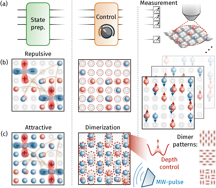
Quantum gas microscopes of ultracold fermionic particles in an optical lattice offer an approach to study the Fermi-Hubbard and related models [20, 21, 22, 23] [Fig. 1(b)]. These experiments offer unprecedented microscopic control and detection of these strongly-correlated quantum systems [24], and major experimental efforts are underway to explore the doped Fermi-Hubbard phase diagram and address outstanding questions regarding -wave superconductivity and quantum magnetism [20, 23]. Such experiments have observed precursors to superconductivity [25, 26, 27, 28, 29, 30] and made consistent progress towards achieving cold effective temperatures where superconductivity is expected [31, 26, 32].
However, challenges remain, including the natural question of how to verify the presence of superconductivity in a quantum gas microscope. One possibility is to indirectly measure superconductivity via transport measurements, similar to traditional solid-state experiments. However, this approach involves additional overhead, since such transport measurements themselves need to be simulated with cold atom techniques, such as with two-terminal [33, 34] experiments.
In this work, we propose a method to directly measure a broad class of observables, including -wave pairing correlators. Our method requires minimal experimental requirements (all of which have been demonstrated) and is applicable in all parameter regimes, while existing proposals hold in certain limits, including where interactions are dominant (the so-called “ limit”) [35] or effectively zero [36, 37, 38].
We use two key concepts: (i) mapping from the repulsive to attractive Hubbard model [40, 41, 42, 43, 44, 45] and (ii) efficient control of the quantum state of fermions on two lattice sites to map previously inaccessible quantities into easily measured ones. We only require the ability to perform the following global operations: partition the lattice into “dimers” of two sites each [46, 36, 37, 38], tune lattice depth after dimerization, perform spin-rotations, and finally make spin-and charge-resolved measurements of each site [47, 48, 49] [Fig. 1(c)]. The protocol is sample-efficient and we use optimal control techniques to optimize its robustness to experimental imperfections.
While -wave pairing is our motivating example, with only five types of global control, the protocol generalizes to any two-site observable that is particle-number preserving. We prove this universality, construct pulse sequences for observables of interest, such as energy density, and discuss their potential applications.
Attractive Hubbard model and pairing correlator.— We use the relationship between the attractive and repulsive Hubbard model to map the pairing correlations into a measurable quantity. In the repulsive model, the superconducting order parameter is of the form : one creates a Cooper pair at sites and , removes a Cooper pair at potentially faraway sites and , and verifies that the system has remained globally phase coherent. Measuring these correlations requires the coherent transport of particles over large distances, a challenging task. Working with the attractive Hubbard model circumvents this issue. The attractive Hubbard model has negative Hubbard interaction and is related to its repulsive counterpart by a particle-hole transformation on the spin-down particles [40, 39]. Crucially, this transforms the above order parameter into . Unlike its repulsive version, this quantity conserves particle number separately on and ; it can be measured through correlations of local spin quantities. Measuring on a low-energy state of the attractive Hubbard model is equivalent to measuring on the corresponding low-energy state of the repulsive Hubbard model. Recent work has utilized this property of the repulsive-to-attractive mapping [35]. Here, we develop a simple protocol to measure such spin correlations with minimal experimental requirements, that applies in any parameter regime.
Measurement protocol.— Our strategy is to transform the desired order parameter into a readily-measured quantity, diagonal in the particle-number basis, via global control. After dimerizing the lattice, we apply a global unitary generated by the time-dependent Hamiltonian
| (1) |
where is the hopping term, restricted to hopping within dimers, is the microwave (MW) spin-flip term, whose time-dependent strengths and are controllable, and is the Hubbard interaction term which we assume has fixed strength . We design a pulse sequence and such that the resultant unitary transforms the desired order parameter into a directly measurable observable. That is, the rotated observable
| (2) |
is diagonal in the measurement basis, where is a spin- and Hermitian-symmetrized variant of (with eigenvalues ): The measured correlations between and give the correlators , in turn equal to the desired pairing correlations up to a factor of 8, see Supplemental Material (SM) [39].
Only a restricted set of controls are available, which constrains the possible unitary transformations. In particular, coherent local control of a quantum gas microscope must preserve particle number, and the resulting unitary cannot couple between particle number sectors of the dimer Hilbert space. In order to measure the desired long-range correlations, one must achieve the transformation Eq. (2) on each sector separately and simultaneously.
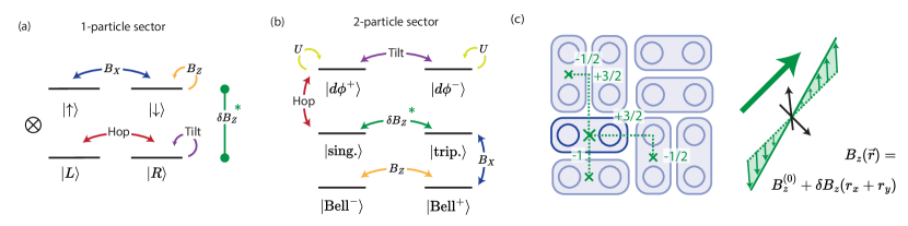
The number sectors are remarkably simple. The 16-dimensional Hilbert space of spin-1/2 fermions on a dimer separates into sectors of 0 to 4 particles, with dimensions 1,4,6,4 and 1 respectively. The 0- and 4-particle sectors are trivial, and the 1- and 3-particle sectors are related by exchanging empty and doubly-occupied sites: a solution on the 1-particle sector is automatically a solution on the 3-particle sector. Therefore, the task simplifies to designing one that simultaneously performs desired transformations on the 1- and 2-particle sectors [Fig. 2(a-c)].
The Hamiltonians in the 1- and 2-particle sectors are:
| (3) | |||
| (4) |
with and the strengths of the hopping and MW controls (suppressing their time-dependence), and the Hubbard interaction strength. We have denoted our basis choice on each sector; we use a non-standard basis on the 2-particle sector. and denote empty and doubly-occupied sites, denote singly-occupied sites, and we have omitted state normalization factors.
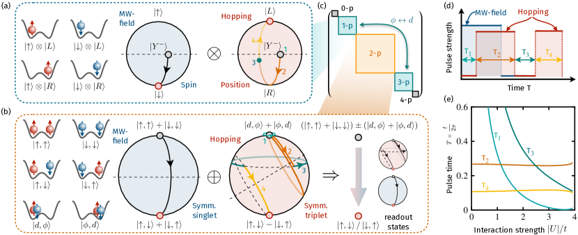
These Hamiltonians are highly structured. First, the 1- and 3-particle Hilbert spaces naturally factorize into positional () and spin () two-level systems, respectively manipulated by hopping and MW controls [Fig. 2(a)]. Meanwhile, the 2-particle Hamiltonian is block-diagonal on the spin-triplet and spin-singlet sectors. The triplet sector is spatially symmetric. Therefore, it is invariant under hopping control , but transforms under MW control . Conversely, the singlet sector transforms under and is invariant under . Further symmetries mean that each control only couples two symmetric states within each spin multiplet [Eq. (4), Fig. 2(b)].
Therefore, our problem can be understood as using hopping and MW control to simultaneously control two qubit degrees of freedom each, in close analogy with the design of the Levine-Pichler entangling gate in neutral-atom quantum computers [50]. Our strategy to achieve Eq. (2) is to design a unitary that maps the eigenstates of onto readout basis states. On the 1-particle sector, the eigenstates of are : the product of Pauli- eigenstates on the spin and positional Bloch spheres. Meanwhile, on the 2-particle sector the nontrivial eigenstates of are , supported entirely on states which are controlled by hopping and MW fields.
As depicted in Fig. 2(a,b), our solution performs the following transformations with MW control:
| (5) | ||||
| (6) |
Meanwhile, we use hopping control to map
| (7) | ||||
| (8) |
Together, Eq. (5-8) map the eigenstates of onto the 1-particle readout basis and the 2-particle states . While hopping and MW control do not provide universal control on their respective two-level systems and hence would not be expected to suffice for general eigenstates, in this case they do give the desired transformations. MW control acts as -axis rotations on its respective 1- and 2-particle Bloch spheres; from Eq. (3,4), a pulse of duration achieves both maps Eq. (5,6). Likewise, hopping acts as an -rotation on its 1-particle Bloch sphere. However, the presence of interactions means that hopping control is no longer a simple -axis rotation on its 2-particle Bloch sphere [Eq. (4), Fig. 2(b)]. Yet, the combination of hopping with a fixed strength and idling with no hopping [] gives universal control on this particular Bloch sphere, allowing us to engineer the map Eq. (8). As discussed in the End Matter (EM), we design a family of trajectories on the Bloch sphere with a tunable parameter, which enables us to find a pulse sequence that performs both maps Eq. (7,8) simultaneously. Our simplest class of solutions with two idling-hopping steps hold for [Fig. 2(d,e)]. Larger values of require sequences with more idling-hopping steps: in the SM we provide solutions up to [39], see also reference code available online [51].
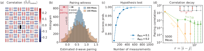
Sample efficiency.— Quantum gas microscopes are constrained by the number of measurements that they can feasibly perform; each experimental run is relatively slow, typically requiring a gas to be cooled to quantum degeneracy. Therefore, it is important to extract useful information with as few measurements as possible. This protocol is provably the most sample-efficient to measure the desired correlations, see SM [39]. Here, we show numerically that a modest number of measurements (thousands or fewer) can resolve signatures of -wave pairing in realistic settings. We simulate two candidate superconducting states: a BCS state with explicitly introduced -wave superconducting order, and the ground state of interacting fermions on a two-legged ladder, obtained through density matrix renormalization group (DMRG) methods (details in SM [39]), and then simulate the estimation of their pairing correlations with the protocol. In Fig. 3(a), we plot the correlations between a central vertical dimer and all other dimers. With only 500 measurement shots, we clearly observe the -wave angular dependence—correlations are positive for vertical-vertical and negative for vertical-horizontal dimer pairs—with minimal statistical noise. Instead of resolving individual correlations, we can also appropriately average over them to quantify -wave order. In Fig. 3(b), we plot the histogram of the estimated -wave order parameter , for 100 and 300 measurements, where encodes the expected angular dependence. For a fixed number of samples, the estimator is a random variable, peaked around its true, non-zero value indicating -wave superconductivity. With small probability, the estimate will be near zero or negative, and one would falsely conclude that -wave superconductivity is absent. Fig. 3(c) demonstrates that only a few hundred measurement shots suffice to achieve success probability for such classification, with a chosen threshold of . Finally, we study -wave pairing in a more realistic setting: the ground state of a two-leg ladder. Unlike the BCS state, here the dimer-dimer correlations decay with their distance. In the superconducting phase, the correlator exhibits a power-law decay over distance , while the Mott-insulating phase exhibits exponentially decaying correlations instead [52]. In Fig. 3(d), we demonstrate that one can observe this phenomenon with 5000 measurements: we accurately reconstruct the power-law/exponential decay of pairing correlations in the ground states of Fermi-Hubbard ladders with average electron density and , respectively.
Optimization and robustness.—

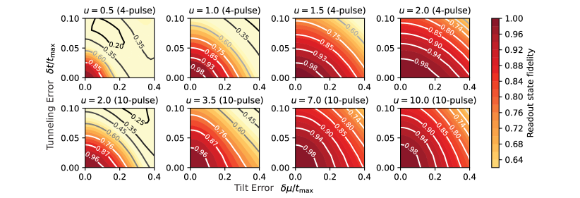
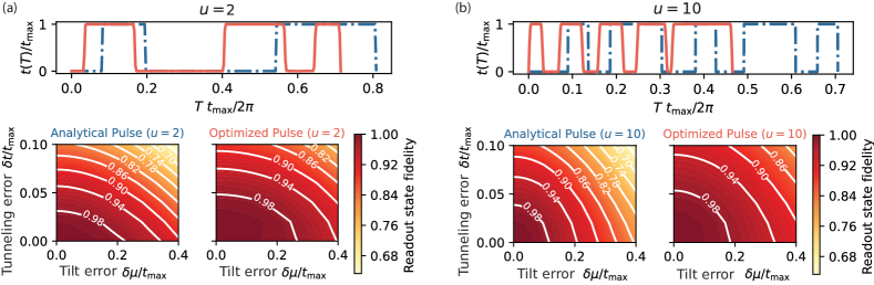
Our pulse sequence is exact under ideal conditions, mapping the eigenstates of the pairing correlator onto Fock states. Here, we analyze the robustness of our pulse sequence to experimental imperfections and develop optimized sequences using optimal control techniques. In particular, we consider two error sources: dimer tilt and hopping strength error. Our analytical solution assumes a uniform chemical potential on the dimer. The presence of a tilt admixes the two states , introducing infidelity. Such tilts may arise from various sources including the harmonic trap used to confine the optical lattice [Fig. 4(a)] or laser speckle [53, 54, 55]. Meanwhile, inhomogeneous hopping strengths lead to different amounts of rotation on each dimer.
We use the optimal control technique of direct collocation [56, 57] to optimize for robustness against these errors. We fix the interaction strength and optimize the hopping pulse between values and a maximum strength . We maximize the fidelity between the target readout states, and initial states (eigenstates of ) evolved in the presence of error, see EM for details. In particular, we target the regime , where the analytic pulse sequences are more sensitive to error. Starting from an analytic solution with five hopping and idling steps interleaved [blue curve in Fig. 4(b)], our optimization yields a smooth pulse (red curve). In Fig. 4(c), we show contour plots of the fidelity over a wide range of error values of tilt and hopping strength : the optimized pulse fidelity is considerably higher than the analytical pulse fidelity, at for experimentally realistic error strengths [58].
Universal control and tomographic completeness.— Finally, this protocol generalizes to measuring a large class of observables. In fact, any number-conserving observable on a dimer can be measured with five types of global control: (i) hopping, (ii) global lattice tilt, (iii) MW drive, (iv) -magnetic field (or optical detuning), and (v) a global gradient in the -magnetic field. Remarkably, each control only couples specific pairs of states (see EM), which allows for the easy design of efficient pulse sequences to measure various quantities, including the kinetic energy and the total energy density across a dimer (SM and reference code [39, 51]). We further explore possible applications of this protocol, namely using global pulse sequences to: (i) perform thermometry in a quantum gas microscope, in which the current approach of comparing against classical simulations is expected to fail at low temperatures, and (ii) enhance the parity readout capabilities commonly seen in quantum gas microscopes [59] to effectively full spin- and charge- resolution [45, 49], see SM [39].
Outlook.— Using hitherto-unnoticed structure in the Hilbert space of spin-1/2 fermions on two sites, we develop an experimental protocol that allows a large class of quantities to be measured, including our motivating example of -wave pairing, only using global controls. We anticipate that this protocol will enable further applications such as variational state preparation [60], and more generally serve as a robust quantum control toolbox for fermionic quantum simulators.
Acknowledgements— We thank the following for insightful discussions: Anant Kale, Aaron Young, Martin Lebrat, Botond Oreg, Carter Turnbaugh, Minh C. Tran, Shang Liu, Zhaoyu Han, Aaron Trowbridge, Andy Goldschmidt, Yi-Zhuang You, Adrian Kantian, Peter Zoller, John Preskill, Sarang Gopalakrishnan, and David Huse. We acknowledge financial support through the Center for Ultracold Atoms, an NSF Physics Frontiers Center (PHY-2317134), the NSF QLCI Award OMA-2016245, the NSF CAREER award 2237244, the Heising-Simons Foundation (grant #2024-4851), and the DOE QUACQ program (DE-SC0025572). C.K. acknowledges support from the NSF through a grant for the ITAMP at Harvard University.
References
- Bluvstein et al. [2024] D. Bluvstein, S. J. Evered, A. A. Geim, S. H. Li, H. Zhou, T. Manovitz, S. Ebadi, M. Cain, M. Kalinowski, D. Hangleiter, et al., Logical quantum processor based on reconfigurable atom arrays, Nature (London) 626, 58 (2024).
- Da Silva et al. [2024] M. Da Silva, C. Ryan-Anderson, J. Bello-Rivas, A. Chernoguzov, J. Dreiling, C. Foltz, F. Frachon, J. Gaebler, T. Gatterman, L. Grans-Samuelsson, et al., Demonstration of logical qubits and repeated error correction with better-than-physical error rates, arXiv:2404.02280 (2024).
- Acharya et al. [2024] R. Acharya, L. Aghababaie-Beni, I. Aleiner, T. I. Andersen, M. Ansmann, F. Arute, K. Arya, A. Asfaw, N. Astrakhantsev, J. Atalaya, et al., Quantum error correction below the surface code threshold, arXiv:2408.13687 (2024).
- Bernien et al. [2017] H. Bernien, S. Schwartz, A. Keesling, H. Levine, A. Omran, H. Pichler, S. Choi, A. S. Zibrov, M. Endres, M. Greiner, et al., Probing many-body dynamics on a 51-atom quantum simulator, Nature (London) 551, 579 (2017).
- Neyenhuis et al. [2017] B. Neyenhuis, J. Zhang, P. W. Hess, J. Smith, A. C. Lee, P. Richerme, Z.-X. Gong, A. V. Gorshkov, and C. Monroe, Observation of prethermalization in long-range interacting spin chains, Science Adv. 3, e1700672 (2017).
- Mi et al. [2021] X. Mi, M. Ippoliti, C. Quintana, A. Greene, Z. Chen, J. Gross, F. Arute, K. Arya, J. Atalaya, R. Babbush, et al., Time-crystalline eigenstate order on a quantum processor, Nature (London) 601, 531 (2021).
- Ebadi et al. [2021] S. Ebadi, T. T. Wang, H. Levine, A. Keesling, G. Semeghini, A. Omran, D. Bluvstein, R. Samajdar, H. Pichler, W. W. Ho, et al., Quantum phases of matter on a 256-atom programmable quantum simulator, Nature (London) 595, 227 (2021).
- Google Quantum AI and Collaborators [2023] Google Quantum AI and Collaborators, Non-Abelian braiding of graph vertices in a superconducting processor, Nature (London) 618, 264 (2023).
- Iqbal et al. [2024] M. Iqbal, N. Tantivasadakarn, R. Verresen, S. L. Campbell, J. M. Dreiling, C. Figgatt, J. P. Gaebler, J. Johansen, M. Mills, S. A. Moses, et al., Non-Abelian topological order and anyons on a trapped-ion processor, Nature (London) 626, 505 (2024).
- Altman et al. [2021] E. Altman, K. R. Brown, G. Carleo, L. D. Carr, E. Demler, C. Chin, B. DeMarco, S. E. Economou, M. A. Eriksson, K.-M. C. Fu, M. Greiner, K. R. Hazzard, R. G. Hulet, A. J. Kollár, B. L. Lev, M. D. Lukin, R. Ma, X. Mi, S. Misra, C. Monroe, K. Murch, Z. Nazario, K.-K. Ni, A. C. Potter, P. Roushan, M. Saffman, M. Schleier-Smith, I. Siddiqi, R. Simmonds, M. Singh, I. Spielman, K. Temme, D. S. Weiss, J. Vučković, V. Vuletić, J. Ye, and M. Zwierlein, Quantum simulators: Architectures and opportunities, PRX Quantum 2, 017003 (2021).
- Emery [1987] V. J. Emery, Theory of high- superconductivity in oxides, Phys. Rev. Lett. 58, 2794 (1987).
- Lee et al. [2006] P. A. Lee, N. Nagaosa, and X.-G. Wen, Doping a Mott insulator: Physics of high-temperature superconductivity, Rev. Mod. Phys. 78, 17 (2006).
- Keimer et al. [2015] B. Keimer, S. A. Kivelson, M. R. Norman, S. Uchida, and J. Zaanen, From quantum matter to high-temperature superconductivity in copper oxides, Nature (London) 518, 179 (2015).
- Bednorz and Müller [1986] J. G. Bednorz and K. A. Müller, Possible high Tc superconductivity in the Ba-La-Cu-O system, Z. Phys. B Cond. Mat. 64, 189 (1986).
- Tsuei and Kirtley [2000] C. C. Tsuei and J. R. Kirtley, Pairing symmetry in cuprate superconductors, Rev. Mod. Phys. 72, 969 (2000).
- Arovas et al. [2022] D. P. Arovas, E. Berg, S. A. Kivelson, and S. Raghu, The Hubbard model, Annu. Rev. Cond. Mat. Phys. 13, 239–274 (2022).
- Qin et al. [2020] M. Qin, C.-M. Chung, H. Shi, E. Vitali, C. Hubig, U. Schollwöck, S. R. White, and S. Zhang (Simons Collaboration on the Many-Electron Problem), Absence of superconductivity in the pure two-dimensional Hubbard model, Phys. Rev. X 10, 031016 (2020).
- Jiang and Devereaux [2019] H.-C. Jiang and T. P. Devereaux, Superconductivity in the doped Hubbard model and its interplay with next-nearest hopping , Science 365, 1424 (2019).
- Xu et al. [2024] H. Xu, C.-M. Chung, M. Qin, U. Schollwöck, S. R. White, and S. Zhang, Coexistence of superconductivity with partially filled stripes in the Hubbard model, Science 384, eadh7691 (2024).
- Esslinger [2010] T. Esslinger, Fermi-Hubbard physics with atoms in an optical lattice, Annu. Rev. Cond. Mat. Phys. 1, 129–152 (2010).
- Gross and Bloch [2017] C. Gross and I. Bloch, Quantum simulations with ultracold atoms in optical lattices, Science 357, 995 (2017).
- Tarruell and Sanchez-Palencia [2018] L. Tarruell and L. Sanchez-Palencia, Quantum simulation of the Hubbard model with ultracold fermions in optical lattices, Comptes Rendus Physique 19, 365 (2018).
- Bohrdt et al. [2021] A. Bohrdt, L. Homeier, C. Reinmoser, E. Demler, and F. Grusdt, Exploration of doped quantum magnets with ultracold atoms, Annals of Physics 435, 168651 (2021).
- Gross and Bakr [2021] C. Gross and W. S. Bakr, Quantum gas microscopy for single atom and spin detection, Nat. Phys. 17, 1316–1323 (2021).
- Hart et al. [2015] R. A. Hart, P. M. Duarte, T.-L. Yang, X. Liu, T. Paiva, E. Khatami, R. T. Scalettar, N. Trivedi, D. A. Huse, and R. G. Hulet, Observation of antiferromagnetic correlations in the Hubbard model with ultracold atoms, Nature (London) 519, 211 (2015).
- Mazurenko et al. [2017] A. Mazurenko, C. S. Chiu, G. Ji, M. F. Parsons, M. Kanász-Nagy, R. Schmidt, F. Grusdt, E. Demler, D. Greif, and M. Greiner, A cold-atom Fermi–Hubbard antiferromagnet, Nature (London) 545, 462 (2017).
- Chiu et al. [2019] C. S. Chiu, G. Ji, A. Bohrdt, M. Xu, M. Knap, E. Demler, F. Grusdt, M. Greiner, and D. Greif, String patterns in the doped Hubbard model, Science 365, 251 (2019).
- Brown et al. [2019] P. T. Brown, D. Mitra, E. Guardado-Sanchez, R. Nourafkan, A. Reymbaut, C.-D. Hébert, S. Bergeron, A.-M. Tremblay, J. Kokalj, D. A. Huse, et al., Bad metallic transport in a cold atom Fermi-Hubbard system, Science 363, 379 (2019).
- Ji et al. [2021] G. Ji, M. Xu, L. H. Kendrick, C. S. Chiu, J. C. Brüggenjürgen, D. Greif, A. Bohrdt, F. Grusdt, E. Demler, M. Lebrat, and M. Greiner, Coupling a mobile hole to an antiferromagnetic spin background: Transient dynamics of a magnetic polaron, Phys. Rev. X 11, 021022 (2021).
- Shao et al. [2024] H.-J. Shao, Y.-X. Wang, D.-Z. Zhu, Y.-S. Zhu, H.-N. Sun, S.-Y. Chen, C. Zhang, Z.-J. Fan, Y. Deng, X.-C. Yao, et al., Antiferromagnetic phase transition in a 3D fermionic Hubbard model, Nature (London) 632, 267 (2024).
- Onofrio [2016] R. Onofrio, Physics of our days: Cooling and thermometry of atomic Fermi gases, Physics-Uspekhi 59, 1129 (2016).
- Spar et al. [2022] B. M. Spar, E. Guardado-Sanchez, S. Chi, Z. Z. Yan, and W. S. Bakr, Realization of a Fermi-Hubbard optical tweezer array, Phys. Rev. Lett. 128, 223202 (2022).
- Chien et al. [2015] C.-C. Chien, S. Peotta, and M. Di Ventra, Quantum transport in ultracold atoms, Nat. Phys. 11, 998–1004 (2015).
- Krinner et al. [2017] S. Krinner, T. Esslinger, and J.-P. Brantut, Two-terminal transport measurements with cold atoms, J. Phys. Cond. Mat. 29, 343003 (2017).
- Schlömer et al. [2024] H. Schlömer, H. Lange, T. Franz, T. Chalopin, P. Bojović, S. Wang, I. Bloch, T. A. Hilker, F. Grusdt, and A. Bohrdt, Local control and mixed dimensions: Exploring high-temperature superconductivity in optical lattices, arXiv:2406.02551 (2024).
- Keßler and Marquardt [2014] S. Keßler and F. Marquardt, Single-site-resolved measurement of the current statistics in optical lattices, Phys. Rev. A 89, 061601 (2014).
- Impertro et al. [2024a] A. Impertro, S. Karch, J. F. Wienand, S. Huh, C. Schweizer, I. Bloch, and M. Aidelsburger, Local readout and control of current and kinetic energy operators in optical lattices, Phys. Rev. Lett. 133, 063401 (2024a).
- Impertro et al. [2024b] A. Impertro, S. Huh, S. Karch, J. F. Wienand, I. Bloch, and M. Aidelsburger, Realization of strongly-interacting Meissner phases in large bosonic flux ladders, arXiv:2412.09481 (2024b).
- [39] See Supplementary Material, which includes References [61, 62, 63, 64, 65, 66, 67, 68, 69, 70, 71, 72, 73, 74, 75, 76, 77, 78, 79, 80, 81, 82, 83, 84].
- Ho et al. [2009] A. Ho, M. Cazalilla, and T. Giamarchi, Quantum simulation of the Hubbard model: The attractive route, Phys. Rev. A 79, 033620 (2009).
- Mitra et al. [2018] D. Mitra, P. T. Brown, E. Guardado-Sanchez, S. S. Kondov, T. Devakul, D. A. Huse, P. Schauß, and W. S. Bakr, Quantum gas microscopy of an attractive Fermi-Hubbard system, Nat. Phys. 14, 173 (2018).
- Chan et al. [2020] C. F. Chan, M. Gall, N. Wurz, and M. Köhl, Pair correlations in the attractive Hubbard model, Phys. Rev. Res. 2, 023210 (2020).
- Gall et al. [2020] M. Gall, C. F. Chan, N. Wurz, and M. Köhl, Simulating a Mott insulator using attractive interaction, Phys. Rev. Lett. 124, 010403 (2020).
- Hartke et al. [2020] T. Hartke, B. Oreg, N. Jia, and M. Zwierlein, Doublon-hole correlations and fluctuation thermometry in a Fermi-Hubbard gas, Phys. Rev. Lett. 125, 113601 (2020).
- Hartke et al. [2023] T. Hartke, B. Oreg, C. Turnbaugh, N. Jia, and M. Zwierlein, Direct observation of nonlocal fermion pairing in an attractive Fermi-Hubbard gas, Science 381, 82 (2023).
- Atala et al. [2013] M. Atala, M. Aidelsburger, J. T. Barreiro, D. Abanin, T. Kitagawa, E. Demler, and I. Bloch, Direct measurement of the zak phase in topological bloch bands, Nat. Phys. 9, 795 (2013).
- Bakr et al. [2009] W. S. Bakr, J. I. Gillen, A. Peng, S. Fölling, and M. Greiner, A quantum gas microscope for detecting single atoms in a Hubbard-regime optical lattice, Nature (London) 462, 74 (2009).
- Boll et al. [2016] M. Boll, T. A. Hilker, G. Salomon, A. Omran, J. Nespolo, L. Pollet, I. Bloch, and C. Gross, Spin-and density-resolved microscopy of antiferromagnetic correlations in Fermi-Hubbard chains, Science 353, 1257 (2016).
- Koepsell et al. [2020] J. Koepsell, S. Hirthe, D. Bourgund, P. Sompet, J. Vijayan, G. Salomon, C. Gross, and I. Bloch, Robust bilayer charge pumping for spin-and density-resolved quantum gas microscopy, Phys. Rev. Lett. 125, 010403 (2020).
- Levine et al. [2019] H. Levine, A. Keesling, G. Semeghini, A. Omran, T. T. Wang, S. Ebadi, H. Bernien, M. Greiner, V. Vuletić, H. Pichler, and M. D. Lukin, Parallel implementation of high-fidelity multiqubit gates with neutral atoms, Phys. Rev. Lett. 123, 170503 (2019).
- [51] Code available online, https://github.com/daniel-k-mark/optical_lattice_control.
- Dolfi et al. [2015] M. Dolfi, B. Bauer, S. Keller, and M. Troyer, Pair correlations in doped Hubbard ladders, Phys. Rev. B 92, 195139 (2015).
- Meyrath et al. [2005] T. P. Meyrath, F. Schreck, J. L. Hanssen, C.-S. Chuu, and M. G. Raizen, Bose-Einstein condensate in a box, Phys. Rev. A 71, 041604 (2005).
- Gaunt et al. [2013] A. L. Gaunt, T. F. Schmidutz, I. Gotlibovych, R. P. Smith, and Z. Hadzibabic, Bose-Einstein condensation of atoms in a uniform potential, Phys. Rev. Lett. 110, 200406 (2013).
- Navon et al. [2021] N. Navon, R. P. Smith, and Z. Hadzibabic, Quantum gases in optical boxes, Nat. Phys. 17, 1334 (2021).
- Trowbridge et al. [2023] A. Trowbridge, A. Bhardwaj, K. He, D. I. Schuster, and Z. Manchester, Direct collocation for quantum optimal control, in 2023 IEEE International Conference on Quantum Computing and Engineering (QCE) (IEEE Computer Society, Los Alamitos, CA, USA, 2023) pp. 1278–1285.
- Propson et al. [2022] T. Propson, B. E. Jackson, J. Koch, Z. Manchester, and D. I. Schuster, Robust quantum optimal control with trajectory optimization, Phys. Rev. Appl. 17, 014036 (2022).
- Lebrat et al. [2024] M. Lebrat, M. Xu, L. H. Kendrick, A. Kale, Y. Gang, P. Seetharaman, I. Morera, E. Khatami, E. Demler, and M. Greiner, Observation of Nagaoka polarons in a Fermi–Hubbard quantum simulator, Nature (London) 629, 317–322 (2024).
- Parsons et al. [2016] M. F. Parsons, A. Mazurenko, C. S. Chiu, G. Ji, D. Greif, and M. Greiner, Site-resolved measurement of the spin-correlation function in the Fermi-Hubbard model, Science 353, 1253 (2016).
- Stanisic et al. [2022] S. Stanisic, J. L. Bosse, F. M. Gambetta, R. A. Santos, W. Mruczkiewicz, T. E. O’Brien, E. Ostby, and A. Montanaro, Observing ground-state properties of the Fermi-Hubbard model using a scalable algorithm on a quantum computer, Nat. Comm. 13, 5743 (2022).
- Ashcroft and Mermin [1976] N. W. Ashcroft and N. D. Mermin, Solid State Physics (Holt-Saunders, 1976).
- Girvin and Yang [2019] S. M. Girvin and K. Yang, Modern Condensed Matter Physics (Cambridge University Press, 2019).
- Mai et al. [2022] P. Mai, S. Karakuzu, G. Balduzzi, S. Johnston, and T. A. Maier, Intertwined spin, charge, and pair correlations in the two-dimensional Hubbard model in the thermodynamic limit, Proc. Nat. Acad. Sci. USA 119, e2112806119 (2022).
- Gong et al. [2021] S. Gong, W. Zhu, and D. N. Sheng, Robust -wave superconductivity in the square-lattice model, Phys. Rev. Lett. 127, 097003 (2021).
- White [1992] S. R. White, Density matrix formulation for quantum renormalization groups, Phys. Rev. Lett. 69, 2863 (1992).
- OEIS Foundation Inc. [2024a] OEIS Foundation Inc., The On-Line Encyclopedia of Integer Sequences (2024a), published electronically at http://oeis.org/A001333.
- OEIS Foundation Inc. [2024b] OEIS Foundation Inc., The On-Line Encyclopedia of Integer Sequences (2024b), published electronically at http://oeis.org/A000129.
- Bickel and Doksum [2015] P. J. Bickel and K. A. Doksum, Mathematical statistics: basic ideas and selected topics, volumes I (Chapman and Hall/CRC, 2015).
- Trowbridge et al. [2023] A. Trowbridge, A. Bhardwaj, K. He, D. I. Schuster, and Z. Manchester, Direct collocation for quantum optimal control, arXiv:2305.03261 (2023).
- Goldschmidt and Chong [2023] A. J. Goldschmidt and F. T. Chong, Automatic pulse-level calibration by tracking observables using iterative learning, arXiv:2304.12166 (2023).
- Leung et al. [2017] N. Leung, M. Abdelhafez, J. Koch, and D. Schuster, Speedup for quantum optimal control from automatic differentiation based on graphics processing units, Phys. Rev. A 95, 042318 (2017).
- Kosut et al. [2022] R. L. Kosut, G. Bhole, and H. Rabitz, Robust quantum control: Analysis & synthesis via averaging, arXiv:2208.14193 (2022).
- Su et al. [2023] L. Su, A. Douglas, M. Szurek, R. Groth, S. F. Ozturk, A. Krahn, A. H. Hébert, G. A. Phelps, S. Ebadi, S. Dickerson, et al., Dipolar quantum solids emerging in a Hubbard quantum simulator, Nature (London) 622, 724 (2023).
- Trotzky et al. [2010] S. Trotzky, Y.-A. Chen, U. Schnorrberger, P. Cheinet, and I. Bloch, Controlling and detecting spin correlations of ultracold atoms in optical lattices, Phys. Rev. Lett. 105, 265303 (2010).
- Zhu et al. [2024] Z. Zhu, Y. Kiefer, S. Jele, M. Gächter, G. Bisson, K. Viebahn, and T. Esslinger, Quantum circuits based on topological pumping in optical lattices, arXiv:2409.02984 (2024).
- Stace [2010] T. M. Stace, Quantum limits of thermometry, Phys. Rev. A 82, 011611 (2010).
- Hovhannisyan and Correa [2018] K. V. Hovhannisyan and L. A. Correa, Measuring the temperature of cold many-body quantum systems, Phys. Rev. B 98, 045101 (2018).
- Mehboudi et al. [2019] M. Mehboudi, A. Sanpera, and L. A. Correa, Thermometry in the quantum regime: recent theoretical progress, J. Phys. A Math. Theor. 52, 303001 (2019).
- Köhl [2006] M. Köhl, Thermometry of fermionic atoms in an optical lattice, Phys. Rev. A 73, 031601 (2006).
- Varney et al. [2009] C. N. Varney, C.-R. Lee, Z. J. Bai, S. Chiesa, M. Jarrell, and R. T. Scalettar, Quantum Monte Carlo study of the two-dimensional fermion Hubbard model, Phys. Rev. B 80, 075116 (2009).
- Young et al. [2022] A. W. Young, W. J. Eckner, N. Schine, A. M. Childs, and A. M. Kaufman, Tweezer-programmable 2d quantum walks in a Hubbard-regime lattice, Science 377, 885 (2022).
- Aidelsburger et al. [2013] M. Aidelsburger, M. Atala, M. Lohse, J. T. Barreiro, B. Paredes, and I. Bloch, Realization of the Hofstadter Hamiltonian with ultracold atoms in optical lattices, Phys. Rev. Lett. 111, 185301 (2013).
- Chung and Peschel [2001] M.-C. Chung and I. Peschel, Density-matrix spectra of solvable fermionic systems, Phys. Rev. B 64, 064412 (2001).
- Fishman et al. [2022] M. Fishman, S. R. White, and E. M. Stoudenmire, The ITensor software library for tensor network calculations, SciPost Phys. Codebases 4 (2022).
- Cheng and Gupta [1989] H. Cheng and K. C. Gupta, An historical note on finite rotations, J. Appl. Mech. 56, 139 (1989).
- Zhang et al. [2014] J. Zhang, L. Greenman, X. Deng, and K. B. Whaley, Robust control pulses design for electron shuttling in solid-state devices, IEEE Transactions on Control Systems Technology 22, 2354 (2014).
- Wu et al. [2017] C. Wu, B. Qi, C. Chen, and D. Dong, Robust learning control design for quantum unitary transformations, IEEE Transactions on Cybernetics 47, 4405 (2017).
- Nocedal et al. [2009] J. Nocedal, A. Wächter, and R. A. Waltz, Adaptive barrier update strategies for nonlinear interior methods, SIAM Journal on Optimization 19, 1674 (2009).
- Wächter and Biegler [2005] A. Wächter and L. T. Biegler, Line search filter methods for nonlinear programming: Local convergence, SIAM Journal on Optimization 16, 32 (2005).
- Byrd et al. [1999] R. H. Byrd, M. E. Hribar, and J. Nocedal, An interior point algorithm for large-scale nonlinear programming, SIAM Journal on Optimization 9, 877 (1999).
- Trowbridge and Bhardwaj [2024] A. Trowbridge and A. Bhardwaj, Quantumcollocation.jl, https://github.com/kestrelquantum/QuantumCollocation.jl (2024).
End matter
Pulse design.—We briefly summarize how to determine our pulse sequence parameters: the pulse durations plotted in Fig. 2(d, e). As discussed in the main text, we have a spin-flip microwave (MW) pulse of strength and duration . This performs a pulse on the 1-particle (1-p) spin states and a pulse on the two levels of the 2-particle (2-p) inversion symmetric, triplet states, mapping and . We also require a non-trivial pulse sequence of hopping strength over time. This performs the mappings on the 1- and 2-p sectors:
| (9) | ||||
| (10) |
where on the 1-p sector, indicates that can be mapped to either or . Taken together, the field and hopping pulses map the eigenstates of onto readout states: and .
As discussed in the main text, the effect of hopping and idling in both 1-/2-p sectors can be visualized on four Bloch spheres [Fig. 2(b,c)]. Our goal is to perform a rotation on the 1-p positional Bloch sphere, while also mapping the north to south pole on the inversion-symmetric, spin-singlet 2-p states. The challenge lies in the fact that in the presence of interactions, hopping results in a rotation on this 2-p Bloch sphere about a tilted axis. To remedy this, we add an idling step, corresponding to a rotation about the vertical axis, to transport between tilted arcs, as illustrated in Fig. 2(c).
We must choose the correct pulse parameters in order to achieve Eq. (9,10) simultaneously. We parametrize the hopping sequence in terms of the angles and that the trajectory traces on the 2-p Bloch sphere; these can be converted to the duration of each step by and . Starting from the north pole, we use the Rodrigues formula [85] to determine the endpoint of the first hopping step in terms of :
| (11) |
where . Similarly, backward-rotating the south pole gives the starting point of the second hopping step:
| (12) |
and can be connected by an idling step if the -coordinates of are equal. This relates and by the equation:
| (13) |
Expressed in this form, it is convenient to incorporate the constraint from the 1-p sector: the total hopping time must equal for some integer , which, in terms of the angles is equivalent to
| (14) |
Combining Eqs. (13,14) gives a nonlinear equation for as a function of and . As mentioned in the main text, choosing gives solutions in the region . The angles [proportional to in Fig. 2(d,e)] immediately determine the rest of the pulse sequence. The idling angle () to connect the two tilted arcs can be obtained from as
| (15) |
Finally, we require an initial idling step, whose angle () is simply the difference between the phases accumulated in the triplet vs. the singlet sector. This ensures that our pulse sequence ends in the desired superpositions . These four angles fully specify our pulse sequence, and their corresponding pulse times are plotted as a function of in Fig. 2(e). In the SM, we discuss pulse sequences valid for larger values of , either with larger values of or pulse sequences with more steps.
Pulse optimization.—We use the method of direct collocation [56, 57] to optimize our pulse sequences for robustness against two sources of error: tilt error , in which the two sites on each dimer have unequal chemical potential, and amplitude error , where the hopping strength , or equivalently interaction strength in a dimer differs from its expected value. We quantify the robustness of our pulse through the fidelity
| (16) |
between the target readout state , and the initial state (i.e. nontrivial eigenstates of the observable ), evolved with an imperfect unitary [86, 87]. We then average the fidelity over the 1-p and 2-p eigenstates, indexed by , and uniformly over a range of error strengths, indexed by . There are multiple ways one could perform this average, but we have verified that this choice does not significantly affect the optimization. A large fidelity would certify that the expectation values measured with the protocol are close to their true value, even in the presence of errors.
Within the framework of directed collocation, we minimize the average infidelity
| (17) |
subject to the constraints that
| (18) | ||||
| (19) | ||||
| (20) | ||||
| (21) | ||||
| (22) |
where we have discretized the unitary into a sequence of unitaries at time-points separated by an interval , with hopping strengths . These unitaries are constrained to satisfy the Schrödinger equation [Eq. (18)], and the initial condition that is the identity [Eq. (19)]. We have also constrained the pulse to be smooth by requiring its first and second derivatives to have magnitudes smaller than and respectively. Our optimization task (17-22) is in the form of a typical nonlinear programming (NLP) problem, and we use an interior-point optimizer (IPOPT) [88, 89, 90] to find a numerical solution. This method has been used in recent quantum optimal control literature [56] and is available online as QuantumCollocation.jl [91].
Compared to gradient-based pulse optimization methods, such as gradient ascent pulse engineering (GRAPE), the directed collocation approach has several advantages: (i) enforcing the Schrödinger dynamics as a constraint enables the solver to explore unphysical regions before converging to an optimal physical trajectory, (ii) it is easy to add additional constraints on the pulse shape (e.g. maximum value and derivatives), and (iii) this approach is compatible with widely available and highly optimized NLP solvers.
Our analytic pulses show a modest degree of robustness to experimental error (Fig. S2 in SM). Unsurprisingly, the more complicated 10-pulse sequences, necessary in the regime , are significantly less robust than the simpler 4-pulse sequences valid for small . As illustrated in Fig. 4, in this regime our optimization scheme shows significant gains, with no additional experimental complexity, achieving over fidelity under realistic values of and .
Universal experimental control set.— We find that five types of global experimental controls allow for universal manipulations of the quantum states on each particle-number sector. These controls are:
-
(i)
Hopping,
-
(ii)
Global lattice tilt,
-
(iii)
Spin-flip MW drive,
-
(iv)
-magnetic field (or optical detuning), and a
-
(v)
Global gradient in the -magnetic field.
This can be seen by directly computing the action of each control on each particle-number sector. For example, in the 2-p sector, we have
where is the hopping strength, is the chemical potential difference (“tilt”) between the sites and of the dimer, and are the average spin-flip and Zeeman fields experienced by the dimer, and is the difference in Zeeman fields across the dimer. Here, we have used the same basis as in Eq. (4). Remarkably, each control selectively couples different states in the 2-p Hilbert space, as is also the case in the 1-/3-p Hilbert space (see SM Fig. S4). Using this selectivity, we explicitly show how any number-preserving observable can be measured using these five controls. We also design efficient pulses to measure specific observables of interest. In all examples we study, we do not need all five controls, as summarized in Table 1.
Finally, we mention a subtlety: we propose to realize the term with a global field gradient. This not only introduces the term, but also shifts the value of from dimer to dimer. Generically, this leads to spatially-varying rotations between the states. However, if we only use the global field gradient to perform -pulses between and , we show in the SM that the action on the subspace is trivial. Despite this restriction, this suffices for our universality argument, and we can also utilize general rotations when the action on the states does not affect the protocol outcome.
| Obs./Gate | Hop. | Tilt | Ref. | |||
|---|---|---|---|---|---|---|
| -wave pairing | ||||||
| Kinetic energy | SM Fig. S5 | |||||
| Energy density | ||||||
| pSWAP | ||||||
| odd-SWAP | SM Fig. S7 | |||||
| Spin-resolved current |
Appendix A Superconducting pairing observables and Bardeen–Cooper–Schrieffer (BCS) theory
In this work, we present a protocol to measure the long-distance correlations of the Cooper pairing creation observable, after a spin-singlet and Hermitian symmetrization and a particle-hole transformation mapping the repulsive to attractive Fermi-Hubbard model. Here, we describe this symmetrization, the repulsive-to-attractive mapping, and describe our numerical methods investigating Bardeen–Cooper–Schrieffer (BCS) states and the ground states of Fermi-Hubbard model on a two-leg ladder.
A.1 Superconducting pairing observables
A signature of superconductivity is the formation of a condensate of fermion pairs. In textbook treatments of superconductivity, a superconducting state is distinguished by a non-zero expectation value of the pairing creation operator [61, 62]. Such a state cannot have fixed particle number, as would be expected in quantum gas microscopes. Instead, superconductivity would manifest in off-diagonal long-range order, i.e. in the correlators taking non-zero value. These correlators can be obtained by the Fourier transform of real-space four point correlators .
Instead of the vanilla pairing operator , we symmetrize the pairing operator as follows:
| (23) |
where creates a singlet on . This has two forms of symmetrization: spin-singlet symmetrization, and Hermitian symmetrization. First of all, since - and -wave superconductivity involve spatially symmetric and hence spin-antisymmetric Cooper pairs, only the singlet pairing function [63, 64] is expected to be non-zero, while the triplet pairing observable will have zero expectation value. The long-range spin-singlet pairing correlator is related to the vanilla pairing correlation by .
This protocol enables the measurement of dimer-dimer correlations of Hermitian observables. This contains the terms
| (24) |
We show that for any thermal state of the Fermi-Hubbard model with fixed particle number. Due to the conservation of particle number, the last two terms in Eq. (24) are always zero. Furthermore, the fact that the Fermi-Hubbard model is time-reversal symmetric implies that . Therefore, the correlations measured in this protocol are equal to .
We remark that for BCS states (discussed below), which are time-reversal symmetric but do not have fixed particle number, one can show with Wick’s theorem that instead, since is non-zero. Therefore, particle-number conservation is a key assumption if one wants to quantitatively estimate . Furthermore, upon the repulsive-to-attractive mapping, particle-number conservation is mapped to magnetization conservation, and the total magnetization may not necessarily be fixed in an experimental state. Fortunately, this assumption is not necessary, after a slight modification of the protocol in this work: by also measuring the correlators where , we can independently estimate and .
We next turn to determining pairing order. -wave and -wave superconductivity can be distinguished by their real-space pairing symmetries. For example, in -wave superconductivity, the pairing correlation does not depend on the relative orientation of and , while in wave superconductivity, the correlator changes sign when the orientation of to is rotated by . Therefore, to distinguish between - and -wave superconductivity, the following spatial symmetrizations can be used:
| (25) |
and the long-range correlations and would distinguish pairing order. This will be the observable we aim to measure, upon a repulsive-to-attractive mapping which we discuss below.
A.2 Repulsive-to-attractive particle-hole transformation
The mapping between repulsive and attractive Fermi-Hubbard models is accomplished by the following particle-hole transformation, which only acts non-trivially on the spin-down particles [40]:
| (26) |
This is a unitary transformation, and the phase factor indicates that this transformation has a sign on one sublattice of a bipartite lattice, here the square lattice. This transformation leaves the operators of the spin-up fermions unchanged, but maps the spin-down occupation operator . With this phase factor, the interaction term changes sign, , while the hopping terms are unchanged. This also exchanges the roles of total particle number with the total magnetization : a low-energy state at a certain filling and zero magnetization on the repulsive Hubbard model would be related by this particle-hole transformation to a low-energy state at half-filling and corresponding magnetization on the attractive Hubbard model.
In momentum space, the mapping can be written as
| (27) |
where with as the lattice spacing. This can be used to obtain different order parameters and corresponding phases transformation between the repulsive () and attractive () Fermi-Hubbard models. In our case of interest, -wave superconductivity in the repulsive Hubbard model, with order parameter gets mapped to -wave anti-ferromagnetic order, with order parameter , see Ref. [40] for more details.
A.3 BCS theory and efficient simulation of BCS states
We describe our numerical simulations performed on Bardeen–Cooper–Schrieffer (BCS) states. These states are toy models for superconducting states, based on BCS theory. The fermionic wavefunction can be written as [61, 62]
| (28) |
where
| (29) |
and the momentum space pairing function is defined as , where the dispersion and gap functions are given respectively by
| (30) |
| (31) |
In our numerical simulations, we use the parameter values and , firmly in the BCS regime of the BCS-BEC (Bose-Einstein condensate) crossover.
Since the BCS wavefunction is a fermionic Gaussian state, its properties are fully determined by its two-fermion correlations. In our numerical simulation, we consider a square lattice with periodic boundary conditions. We use the following useful correlations:
| (32) |
Since there is no spin-triplet pairing, . Furthermore, the state has magnetization 0, and hence . Finally, using Wick’s theorem, we calculate the four-fermion correlators:
| (33) |
A.3.1 Reduced density matrix of a fermionic bilinear state
In our numerical simulations, we evaluate the spatial correlations on the BCS state by computing its reduced density matrix supported on the neighborhood of and .
Given a fermionic bilinear wave function
| (34) |
where matrix denotes the fermion pairing in the real space, one can efficiently calculate its reduced density matrix on a subsystem . We rearrange the pairing matrix into four sub-matrices: , , and depending on whether the index are in the region or its complement . Then the reduced density matrix can be written as [83]
| (35) |
with
| (36) |
where is the matrix transpose of . This can be shown by calculating the overlap of the reduced density matrix with the fermionic coherent states as
| (37) |
with
| (38) |
This results in
| (39) |
A detailed derivation can be found in Ref. [83], and one should notice a sign difference between the definition in Eq. (36) for and the one in Ref. [83].
In our numerical simulations of a lattice system with the periodic boundary condition, we transform the BCS wavefunction into real space with bilinear form Eq. (34) by using two spinless fermions to represent one spinful fermion. We then apply Eq. (35) to get the reduced density matrix. A point of note is that when using Eq. (35), the definition of should be the same as Eq. (34), and the extra coefficient cannot be absorbed into the normalization constant . In order to simulate measurements on a state with the attractive Fermi-Hubbard model, we use the particle-hole transformation Eq. (26). One can show that one can take the partial trace before or after the particle-hole transformation. In our case, we first obtain the reduced density matrix from Eq. (35) before applying the particle-hole transformation.
In all the simulations with the BCS state, we choose the system to be a square lattice, comparable in size to typical experiments.
A.4 Ground state of Fermi-Hubbard ladders
In this work, we numerically study the ground state of the Fermi-Hubbard model on a two-leg ladder with length (obtained with density matrix renormalization group (DMRG) methods [65]), as a more realistic state than BCS states. On the repulsive Hubbard model, we observe (i) power-law decay of pairing correlations at average electron density ( spin-up electrons and spin-down electrons) with , and (ii) exponentially-decaying correlations at half filling ( spin-up electrons and spin-down electrons) with . On the attractive Fermi-Hubbard model, this corresponds to (i) spin-up electrons and spin-down electrons with and (ii) spin-up electrons and spin-down electrons with . We set the maximum bond dimensions to be 1800 for the hole-doped state and 900 for the half-filled state, implemented with the ITensor.jl package [84]. Similar parameters are also used in Ref. [52].
Appendix B Parameters for hopping pulse sequences
Here, we describe our analytic solution to the hopping pulse sequence to measure wave pairing correlations. To restate our approach outlined in the main text, we develop pulse sequences that map the eigenstates of the observable of interest to the readout basis. The -wave pairing observable, Eq. (23), has nontrivial eigenstates in the 1-p, 2-p, and 3-p sectors:
| Eigenvalue | Eigenstate | Readout state |
|---|---|---|
As stated in the main text, the MW pulse is simple: a pulse of duration effects a -rotation on the spin Bloch sphere in the 1-p and 3-p sectors, and performs a -rotation on the triplet, inversion-symmetric 2-p Bloch sphere, sending the state to . It remains to design a pulse sequence of hopping strength over time, that effects a -rotation on the positional Bloch spheres in the 1-p and 3-p sectors, simultaneously with a -rotation on the singlet, inversion-symmetric 2-p Bloch sphere.
The pulse sequence that achieves this goal, which we dub Hop+U1, will turn out to be useful not just to measure wave pairing. In Appendix F, we develop pulse sequences to measure other quantities of interest, including the kinetic energy and energy density. These sequences make use of Hop+U1 extensively, in conjunction with the other types of experimental control discussed in Appendix E.
This pulse sequence achieves the mappings on the 1-p and 2-p sectors
| (40) | ||||
| (41) |
where on the 1-p sector, denotes that the state can be mapped to either or . For simplicity, we assume that we only have the ability to toggle the hopping strength off or on, i.e. between the values and . Meanwhile, we assume that the interaction strength is always fixed to a value of .
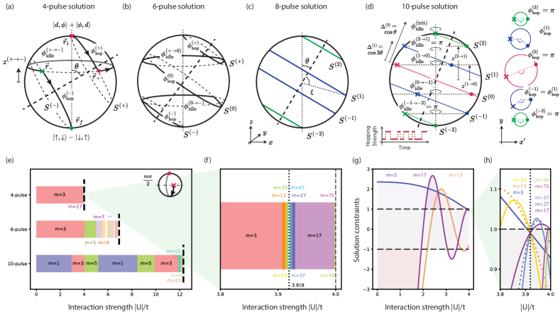
Under idling and hopping, the dynamics on the 2-p sector is only nontrivial on the two-level system formed by the states , and designing the mapping Eq. (41) is equivalent to designing a trajectory on the equivalent Bloch sphere. Our pulse sequences will depend on the ratio of . In particular, our simplest pulse sequence has four steps: idling, hopping, idling and hopping for different amounts of time. On the Bloch sphere, idling gives rise to trajectories on horizontal arcs, while hopping results in trajectories on tilted arcs. The simple four-pulse sequences correspond to connecting two tilted circles that intersect the north and south poles with a single horizontal circle [Fig. S1(a)]. Geometrically, this is only possible when .
Even within this feasible range , the parameters of the four-pulse sequence, i.e. the duration of each step, depend on the value of . In Appendix B.2 we describe how to determine these parameters. Our solutions for the four-pulse sequences depend on an integer describing the amount of over-rotation on the 1-p positional Bloch sphere. Solutions exist for the simplest case when . In the rest of the feasible range , we determine an infinite sequence of integers for which solutions exist. We then seek to develop pulse sequences in the experimentally relevant regime . In Appendix B.3, we study more complex 6-,8- and 10-pulse sequences [Fig. S1(b-d)] that provide solutions for larger values of , providing solutions for their pulse parameters.
Our pulse sequence solutions hold regardless of the sign of or : such sign changes result in axes of rotation that are either reflected about the plane of the Bloch sphere, or with reversed rotation directions. The resulting trajectories in the Bloch sphere are simply reflected versions of the trajectory with positive and . Therefore, without loss of generality, we take and to be positive.
Finally, we remark on our assumption that the interaction strength is fixed. In reality, it can change when hopping is toggled on and off, since a deeper lattice may have more narrow motional eigenstates and hence doublons may experience stronger interaction when hopping is turned off. In this case, a simple modification suffices: we rescale the idling times appropriately by the modified interaction strength .
B.1 General strategy
For all -pulse solutions, our analysis follows three steps. The pulse sequences are specified by the positions of the arcs along the tilted axis, as well as the heights where and are connected vertically [Fig. S1(a-d)]. The analysis steps are:
-
1.
Given heights and positions , determine the required angles along the arcs using the Rodrigues formula [85]. We then match the required evolution time in the 2-particle sector (LHS) with that of the 1-particle sector (RHS).
(42) where is an odd integer describing the overrotation in the 1-particle sector. This is the only nontrivial step, at which there may not be a solution. For -pulse sequences with large , there may be many degrees of freedom, and we can arbitrarily fix some of their values (equivalently, fix the angles ), as we do in App. B.3.
-
2.
Once is determined, the entire trajectory is specified and we can immediately determine the idling times by computing the angle between the position vectors and , the final and initial points on the Bloch sphere of the arcs and respectively.
-
3.
Finally, we fix the accumulated phase to match the phase accumulated during the magnetic field pulse with an additional idling time at the start of the sequence. This is the only step in which quantum mechanical calculations on (as opposed to on the sphere ) is required.
B.2 Four-pulse sequence
Here, we outline in detail the analysis to solve for the pulse parameters in the measurement sequence for -wave pairing. The essential steps have been condensed in the End Matter (EM), and here we give an extended presentation. For fixed values of interaction strength and tunable hopping strength , the protocol involves four steps: (i) idling for time , (ii) hopping for time , (iii) idling for time , and finally (iv) hopping for time , which we label as in the main text. We derive and provide analytic expressions for these times, for , and in Appendix B.3 we discuss necessary modifications to the protocol for larger values of . The pulse duration of each step is determined by the angle of its arcs on the Bloch sphere. We first solve for the angles of the hopping arcs , which yields the idling angle . Finally, the angle of the first idling step is computed to offset the total dynamical phase accumulated. The physical durations of each pulse are related to their respective angles by
| (43) | |||
| (44) |
where the factor of two is due to the spin-1/2 nature of the Bloch sphere.
To summarize our results for this simplest protocol, we have, as plotted in Fig. 2(e),
| (45) | ||||
| (46) | ||||
| (47) | ||||
| (48) |
valid for . These parameters are respectively obtained from Eqs. (53, 54, 57, 60), where are defined in Eqs. (50, 52), and , and the unitaries are defined in Eqs. (59, 60).
B.2.1 Hopping times
We solve for the hopping angles by utilizing the Rodriguez rotation formula [85]. It states that in three dimensions, rotating a vector by an angle about an axis gives the new vector
| (49) |
The values of and fix the rotation axis . Given this, we parameterize the trajectory on the Bloch sphere in terms of rotation angles and about . On the Bloch sphere, we have initial and final points and . The rotation by the first hopping step gives
| (50) |
This equation is equivalent to the parametric equation of the tilted arc (with position , here equal to ):
| (51) |
Likewise, rotating by gives
| (52) |
Matching the -coordinates of and [the third entries of Eq. (50) and (52)] gives a relation between and , which can be written as . Finally, the dynamics in the 1-particle sector constrains the total hopping angle
| (53) |
where is a free parameter taking odd-integer values, representing the amount of overrotation on the 1-p Bloch sphere. This gives the equation
| (54) |
which allows us to solve for as a function of . For each , Eq. (54) has solutions as long as the following inequality is satisfied
| (55) |
As mentioned in the main text, does not have any solutions. However, setting yields a solution in the range , illustrated in Fig. S1(e,g).
As a technical point, we may achieve solutions for almost any with different values of [Fig. S1(f)]. To illustrate this, we consider the point . There is a valid solution of to Eq. (54) as long as , where is an integer. In other words, we seek a rational approximation , with odd numerator . The sequence of best rational approximations to is well studied, and is given by [66, 67]
| (56) |
which guides our search for over-rotation integers . For example, while the cases and do not yield new solutions, while extends the range of validity to , and covers the range [Fig. S1(f)]. While there is no solution at exactly , since we can achieve arbitrarily precise rational approximations of (or any other number), we can achieve a solution for almost any value of .
We say almost any value because there are isolated points for which there is no solution. If is an irrational number and , will densely fill the interval over all odd , and hence there are values of that satisfy the inequality Eq. (54). However, there are certain values of for which there is no solution to Eq. (54). For example, precisely at the point , the quantity takes on five distinct values, , all of which have magnitude smaller than . Around this special point however, the sequences and provides solutions [Fig. S1(f)]. One can also verify that and are similar exceptional points. Finally, we emphasize that these higher over-rotation sequences are likely only of theoretical interest; in practice, they are superseded by simpler protocols with more pulse steps, discussed below in Appendix B.3.
B.2.2 Idling times
Using our solutions of Eq. (54), we can immediately solve for the idling angle from the vectors and [Eqs. (50, 52)], projected onto the plane, and using both the dot and cross product to fully resolve the angle :
| (57) |
Finally, is obtained by equating the dynamical phases accumulated in the singlet Bloch sphere (by the lattice depth pulse) and in the triplet Bloch sphere (by the MW pulse). These phases are most easily computed by multiplying the unitaries from each step to obtain the total phase accumulated. With , we have eigenvalues , with , and eigenstates
| (58) |
with the angle of the rotation axis from the vertical. Exponentiating , we obtain the unitary
| (59) |
The phase accumulated during the idling step is exactly , therefore
| (60) |
where we represent the states and on the Bloch sphere, and is the phase accumulated by the field step [as can be verified by setting in Eq. (59)].
B.3 -pulse sequences
Here, we describe pulse sequences with larger number of steps, which allow for the measurement of the superconducting order parameter at larger values of . As established above, our pulse sequence in its simplest incarnation is valid for and may be extended up to . Beyond , the protocol should be modified, by introducing tilted arcs connected by vertical arcs. Below, we examine the cases , which we refer to as 6-, 8- and 10-pulse sequences. These pulse sequences have more degrees of freedom and we therefore restrict ourselves to solutions with a high degree of symmetry [Fig. S1(b,c,d)], which simplifies our analysis below.
B.3.1 6-pulse sequence
We first discuss a 6-pulse sequence: comprising 3 tilted arcs connected by 2 vertical arcs [Fig. S1(b)]. Such sequences are potentially valid up to , above which the three tilted arcs cannot be made to vertically overlap. Our simplest two solutions are valid for and respectively, and increasing the amount of over-rotation again yields solutions for the entire interval . Although the space of possible sequences is larger, here we restrict ourselves to a class of symmetric pulses which are simpler to analyze, surprisingly even simpler than the four-pulse sequence discussed in the main text.
We consider three tilted arcs. The first and third arcs, and , are fixed to intersect the north and south poles of the Bloch sphere respectively, but we have freedom to place the middle arc anywhere in between. For simplicity, we choose to place on the ‘tilted’ equator [Fig. S1(b)].
As in the four-pulse sequence, our solution consists of angles on the tilted arcs, which can be used to determine the idling angles . We make the following crucial simplifying assumptions: we choose a symmetric solution , and we set [Fig. S1(b)]. In analogy to Eq. (53), matching the required hopping times between 1- and 2-particle sectors gives the equation
| (61) |
for odd integer , which directly allows us to solve for . In order to check the validity of the solution, we also note that for a given , only a range of angles are valid, in the sense that they vertically overlap with the central tilted arc . The value satisfies
| (62) |
As with Eq. (54), there is no solution for . The case admits solutions for , and includes the interval . As with the four-pulse sequences, solutions across the entire range exist for sufficiently large . In this case, however, every larger value of monotonically increases the feasible range, up to the point [Fig. S1(e)]. Precisely at this point, there is no solution, but unlike the four-pulse case, there are no other exceptional points within the interval for which no solutions exist.
B.3.2 8- and 10-pulse sequences
We next move on to discuss higher-pulse sequences, with the aim of providing a concrete sequence in the regime . To do so, we examine the feasibility regions of 8- and 10-pulse sequences. We first examine its ‘feasibility regions’, i.e. the maximum for which these sequences are possible. As above, we restrict ourselves to solutions where the tilted arcs are symmetric about the equator. In the 8- and 10-pulse cases respectively, we consider symmetrically-placed arcs and [Fig. S1(c)]. In the 10-pulse case, there is an additional middle arc which we fix to be on the tilted equator [Fig. S1(d)].
In both case, the locations of arcs and are specified by two numbers: and , i.e. their heights along the tilted axis [Fig. S1(d)]. is fixed by demanding that it intersects with the north pole of the Bloch sphere, this gives . We have two constraints on : (i) that and overlap vertically at height , and that (ii) and overlap at height , or and overlap vertically at height in the 8- and 10-pulse cases respectively. With , constraint (i) can be written as
| (63) |
where is the conical angle of with the tilt axis [Fig. S1(c)]. Meanwhile, constraint (ii) can be written as
| (8-pulse) | (64) | |||
| (10-pulse) | (65) |
Combining these constraints, we find that 8- and 10-pulse solutions could exist for and respectively. Since we seek solutions for the regime , we focus on the 10-pulse sequence in the rest of this section, following the steps outlined in App. B.1. We have three free parameters in the 10-pulse solution: the vertical heights and where the arcs intersect, and the position of along the tilt axis, . For simplicity, we fix , i.e. at the lower end of the range specified by Eq. (65). This fixes and , since it connects the lowest point of with the highest point of . Additionally, we design the path symmetrically such that the paths on are the same, as are those on , and that , illustrated in Fig. S1(d). This leaves as the only free parameter, which is in turn fixed by matching the 1- and 2-particle sectors:
| (66) |
for an odd integer. There is an additional constraint that there be a path from the endpoint on to , which is equivalent to
| (67) |
with , , and given by Eq. (66). For , Eq. (67) is satisfied for , for , , and for , , as illustrated in Fig. S1(e). As with the four- and six-pulse cases, with arbitrarily large one can cover (almost every point in) the entire feasible range .
Appendix C Optimal sample complexity for estimating observable expectation values
Here, we prove that to estimate the expectation value of an observable , the optimal measurement one can perform is the approach we take in this work: to measure in its eigenbasis . While this appears to be a fairly basic fact in quantum estimation theory, we have not found it elsewhere in the literature, hence we provide a self-contained proof here.
We consider the following setting: given a Hermitian observable , consider the positive operator-valued measure (POVM) consisting of elements . A finite number of measurements with this POVM on the state yields a noisy estimate . We ask about the sample complexity of estimating , i.e. the variance in the estimates as a function of the number of samples . We show that the POVM consisting of projectors onto the eigenbasis of , yields an unbiased estimator of with the smallest sample complexity over all POVMs which can estimate .
We analyze the sample complexity of estimating with an arbitrary POVM , i.e. where are positive semi-definite Hermitian operators that sum to the identity, . From total measurements with this POVM, we obtain counts , i.e. the number of times each element is observed, satisfying . The counts are weakly correlated random integers following the multinomial distribution [68]
| (68) |
The expectation value can be estimated from our POVM for all , if and only if can be expressed as a linear combination of the elements . That is, there are real coefficients such that . Then, the estimate of is
| (69) |
As an example, for the POVM (here, we reserve the index to label the eigenbasis), we have , the eigenvalue . Here, as expected, our estimator is .
Using the fact that for multinomial distributions , we can verify that Eq. (69) is an unbiased estimator of . Using the covariances of the multinomial distribution , the uncertainty in our estimate is given by:
| (70) | ||||
| (71) |
We can immediately see that the POVM has a sample complexity equal to the variance of on the state :
| (72) |
We now prove that Eq. (72) is a lower bound for Eq. (71), i.e. projectors on the eigenbasis have the optimal sample complexity over all POVMs that can estimate . The positive semi-definiteness of allows us to write in terms of possible rectangular matrices . It suffices to show that for every pure state ,
| (73) |
To do so, we use the Cauchy-Schwarz inequality on the left-hand-side, noting that for any normalized state ,
| (74) |
where since , we have . Finally, setting gives for the right hand side of Eq. (74), equal to the desired inequality Eq. (73).
Appendix D Optimization for pulse robustness with direct collocation
In this section, we describe our robust pulse optimization procedure using the quantum optimal control method of direct collocation. We first study the robustness of our analytical pulses under the tilt error and hopping error , for different values. In Appendix B, we discussed -pulse analytical sequences valid for different values of . In Fig. S2, we show the contour plots of the state fidelity for 4-pulse and 10-pulse solutions at different values of . As one might expect, sequences with fewer pulses are more robust at the same value of . In Fig. 4, we chose to work in the regime , relevant for typical experiments, and we demonstrated how the analytical 10-pulse solution can be significantly optimized. Here, we describe how we perform this optimization with quantum optimal control techniques.
The quantum control problem can be formulated as an optimization problem in the time-dependent state trajectories subject to the Schrödinger equation. The unitary propagator evolves as
| (75) |
where are trainable pulse parameters. Similar to most quantum optimal control approaches, we set the Hamiltonian to be , where is the drift term that cannot be tuned, and are controllable Hamiltonians whose strengths can be tuned via . In our setup, the drift term would be the Hubbard interaction term , and tunable terms are the hopping and magnetic field terms. Since the magnetic field commutes with the rest of the Hamiltonian, we do not need to analyze it in our problem, and we only focus on the control of the hopping Hamiltonian with strength
| (76) |
We discretize the time interval into points separated by intervals , and we use and to denote the unitary and hopping strength at the -th time point. Then the quantum optimal control problem can be formulated as the following optimization problem [56, 57]:
| (77) |
where is the loss function that depends on the goal of quantum controls. For our purposes, we use the state infidelity as our loss function:
| (78) |
where (initial states) are the nontrivial eigenstates of observables , and (final states) are the readout states. Since the 1-particle and 3-particle sector are dual to each other, we only need to keep the 4 nontrivial eigenstates from the 1-particle sector and 2 nontrivial eigenstates from the 2-particle sector, i.e. . Unlike gradient-based quantum optimal control methods, direct collocation treats the unitary and pulse parameters as separate variables, related by the Schrödinger equation as a constraint. Therefore, one can rewrite the above optimization problem to
| (79) |
where the last two constraints are optional but enforce the smoothness of the pulse. This is in the form of a typical nonlinear programming (NLP) problem:
| (80) |
There are different methods for solving such an NLP. Since most optimization solvers only support real numbers, one needs to first map the complex-valued quantum optimization into a real-valued variable optimization. This can be done by using the isomorphic representation of quantum states and Hamiltonians [71]:
| (81) |
so that . In particular, we use the interior-point optimizer (IPOPT) [88, 89, 90] for solving such an NLP, which has been used in recent quantum optimal control literature [56] and is available open-source as QuantumCollocation.jl [91].
Enforcing dynamical equations as constraints in the optimization procedure is a key idea in direct collocation; it enables the solver to explore unphysical regions during the optimization before converging to an optimal physical trajectory. Compared to gradient-based pulse optimization methods such as gradient ascent pulse engineering (GRAPE), it has several advantages: (i) it has better convergence by utilizing unphysical solutions during optimization, (ii) it is easy to add different types of constraints on the pulse shape (e.g. maximum value and derivatives), and (iii) it is compatible with NLP solvers that are commonly used and highly optimized.
In our optimization, we fix the Hubbard interaction and treat the hopping strengths as trainable parameters, where is time. We allow the hopping strength to take values between 0 and a maximum value . We want the optimal pulse to be robust against tilt error and hopping error . During the optimization, we use the analytical solution as a warm start, and we set the maximum to be slightly larger than the height of the warm-start pulse. To find robust pulses, we use the idea of error sampling [86, 87]. In this approach, the system with an error can be modeled as , where is the Hubbard interaction, is the hopping Hamiltonian, is the tilt chemical potential, and , are the error strengths. Even though the error strength can be stochastic, it has been shown that if the optimal pulse is robust to a range of error strengths, it is also robust to stochastic, potentially time-dependent, errors [72]. Therefore, we keep and constant during the unitary evolution in our optimization. We sample and uniformly from a range of values, and , and use the average state infidelity as the loss function:
| (82) |
where indexes the sampled error strengths (discretized to values). During our optimization, we first set the constraints on the first and second order derivatives of to be large or infinity such that the solver converges to a robust pulse. Then we gradually enforce the first and second order derivatives constraints without jeopardizing the averaged state fidelity such that the optimal pulse is smoother but also robust. In Fig. S3, we plot two optimized pulses for (starting from the four-pulse solution) and (starting from the 10-pulse solution). In both cases, we see marked improvements in robustness compared to our analytical pulses; the optimized pulses we find are also faster and hence may be more robust to other types of error such as decoherence.
Appendix E Universal experimental control set
In Appendix B, we designed our first nontrivial pulse sequence Hop+U1 using a combination of hopping and idling. These sequences can be understood by their effects on the Hilbert space of each particle number sector. On the 1-p sector, hopping performs an axis rotation on the positional Bloch sphere and idling has no effect. Meanwhile, on the 2-p sector, hopping and idling enable arbitrary control on the two-level system. It is natural to ask whether the entire Hilbert space of each particle number sector can be manipulated with other types of global control. Here, we analyze a set of global experimental controls, acting on dimers, which together offer full control over the Hilbert space of each particle number sector. Surprisingly, only five experimental controls suffice, in conjunction with a Hubbard interaction that we assume is always fixed. Furthermore, each type of control selectively couples certain states in Hilbert space, illustrated in Fig. S4(a,b), which allows us to design pulse sequences that effect desired transformations. In this section, we analyze this universal control set and prove its universality.
E.1 Universal control set
Our universal control set comprises of:
-
1.
Hopping strength ,
-
2.
Dimer tilt ,
-
3.
Global MW field ,
-
4.
Global -magnetic (or optical detuning) field ,
-
5.
Global -magnetic field gradient ,
where , are the differences in chemical potential and magnetic field respectively, and , are the average and fields experienced by the dimer, and we explicitly write the Hamiltonian of each control acting on the dimer sites and .
In Fig. S4(a,b), we list the actions of these controls on the 1-p and 2-p Hilbert space. On the 1-p Hilbert space, the fields and naturally act on the spin two-level system, while hopping and tilt are the analogues of and on the positional two-level system. Meanwhile, the field gradient generates entangling -type interactions between the spin and position degrees of freedom: a gradient of the MW field strength would also entangle spin and position: we do not list this here because it can be generated from 3., 4. and 5.
In detail, the Hamiltonian on the dimer, with all controls included, has the following matrix elements in the 1-p, 2-p, and 3-p sectors:
| (83) | ||||
| (84) | ||||
| (85) |
where the 1-p basis is , the 2-p basis is , and the 3-p basis is . We have also used the Fock basis convention where we order the fermion creation operators first by site, before ordering them by spin. To illustrate, some non-trivial readout basis elements are, in terms of fermion creation operators acting on the vacuum:
| (86) | ||||
| (87) |
This site-first convention respects locality and conforms with our intuitions (for example, under this convention, is part of the multiplet which transforms under magnetic field as a spin-1 triplet).
The Hamiltonian in the 2-p sector is particularly simple in the control basis
| (88) | ||||
| (89) | ||||
| (90) |
In this basis, the Hamiltonian is
| (91) |
as we graphically depict in Fig. S4(a,b). Eq. (91) is remarkably simple: each control only couples a specific pair of states in the 2-p manifold. This offers selective control of the control basis states in the 2-p sector, as indicated in Fig. S4(b). Applying pulses of the various control knobs, in a specific order, allows for the measurement of arbitrary observables in this sector. We prove this general statement in Appendix E.2, and proceed to design efficient pulse sequences to measure various quantities in Appendix F.
Finally we remark on a symmetry in the Hilbert space of the 2-p states. The 2-p basis naturally decomposes into two sets of three states: spin-singlet states , and spin-triplet states . While the singlet and triplet symmetry sectors have different multiplicities in spin-1/2 systems, with fermions on a dimer they have three states each and exhibit a remarkable symmetry under positional and spin controls. The spin-singlet states are by definition insensitive to magnetic field, yet couple when the lattice is manipulated with hopping or tilt. Meanwhile, the spin-triplet states mix under magnetic field, but are permutation invariant under exchange of the dimer sites, and hence are invariant under lattice control. These sectors are coupled by the magnetic field gradient, which mixes the positional and spin degrees of freedom. Their symmetry is broken by the presence of the Hubbard interaction, which adds an additional term on that is not present in . However, a ferromagnetic interaction would restore the singlet-triplet symmetry: it would give an additional energy to the states analogous to the Hubbard term on . Ferromagnetic interactions could be realized with, for example, magnetic atoms in optical lattices [73] and may offer avenues for more efficient control, since we would have full two-level system control on both and . However, such systems are relatively uncommon and we emphasize that even without ferromagnetic interaction, our control set is already universal and allow for efficient pulse sequence for all observables that we study in this work. One possible exception could be enabling a SWAP gate in which all number sectors gain an equal phase, as opposed to pSWAP, where the number sectors get imprinted with non-trivial phases (see Appendix F.4.1).
E.1.1 Magnetic field gradient
As mentioned in the End Matter there is a subtlety with using dimer tilt and magnetic-field gradient (or gradient in an optical detuning field). These gradients can be implemented either with a sawtooth profile of chemical potential and field, or with a global gradient. The latter approach is experimentally simpler, but brings with it the challenge that the average chemical potential and field changes from dimer to dimer. The varying chemical potential does not affect the dynamics, since all dynamics on each dimer is block-diagonal in particle number. However, the varying field poses a problem, since there are non-trivial couplings between the triplet states on top of the desired singlet-triplet coupling. This would lead to varying amounts of spin rotation on each dimer across the lattice.
These varying spin rotations can be set to zero due to a fortunate coincidence on the square lattice. In the presence of a gradient, the field is of the form , where is the gradient vector and is the field at a reference point. The midpoints of each dimer are of the form (horizontal dimer) or (vertical dimer) where and are integers and is the lattice spacing. We apply the field gradient along the diagonal of the and plane. Then the field at the midpoint of each dimer (i.e. average field experienced) is
| (92) |
for some integer . That is, the field strengths across all dimers are offset by integer multiples of , for all pairs of dimers, even with different orientations, see Fig. S4(c). Meanwhile, the local gradient at each dimer is also for both horizontal and vertical dimers. The key difference is that in Eq. (91), the average field has a factor of two strength relative to the gradient . Therefore we can use a global uniform gradient to effect a -pulse between and , while performing a trivial operation (pulse) on . Note however, that in the 1-p basis, this will result in a field -pulse being applied on half the dimers. This can usually be taken into account during the data-processing step.
Taken together, this establishes that a global field gradient allows for selective swaps between the and states to be performed. This will be sufficient for most of our purposes. A notable exception is our pulse sequence to measure the energy density (Appendix F.2), where we require a partial singlet-triplet oscillation, i.e. a pulse between and . This does not pose further complications to us since in that protocol, the states and not used and never interact with the other states.
E.2 Proof of universality
Having introduced our control toolset, we proceed to establish that it is universal. Specifically, we establish that any 1-p, 2-p or 3-p observable on a dimer can be measured with our scheme. By this we mean that any 1-/2-/3-p state, which we take to be an eigenstate of an observable, can be mapped into a readout basis state.
This result is almost immediate from Fig. S4(a,b). In the 1- and 3-p sectors, the position and spin two-level systems can be thought of as two qubits. The field gradient provides an entangling gate between them, while hopping/tilt and and fields provide single-qubit control of each two-level system. Taken together, these ingredients allows for arbitrary two-qubit control, in particular the ability to map any state into a readout basis (i.e. computational basis) state.
In the 2-p sector, it is convenient to consider the inverse process, i.e. the ability to prepare any state on the 6-dimensional 2-p Hilbert space from an initial readout basis state, specifically . Our approach will be as follows: (i) first we map into the control basis state . (ii) Next, the combination of hopping and idling provides the ability to prepare any state on the two-level system spanned by . We control this two level system and use -pulses of the other controls to sequentially transfer amplitude into each control basis state.
Step (i) can be accomplished by the sequence:
| (93) |
Next, we describe step (ii). Let the desired 2-p state be in the control basis (without loss of generality, with real and positive). After step (i), the state is . Using hopping and idling, we prepare the state . We then perform pulses with , , and in order, which will result in the state . Each pulse includes a factor of , which was why we initially included a factor of . We proceed iteratively, preparing the state , which we then map . Repeating this process prepares the state . We next prepare the amplitude on with , where . We then swap population to . Finally, a hopping pulse gives the state , and idling for an appropriate amount of time fixes the phases on and gives the desired state .
The above result is sufficient to measure any observable expectation value on a dimer. However, it is not sufficient to measure dimer-dimer correlation functions, as we do in the rest of this work. While an extended universality argument can be made demonstrating that any pair of 1-p and 2-p states can be mapped into readout states using the same pulse, but we omit its details since it is not the focus of this work.
Finally, we emphasize that this construction is fairly inefficient: the sequences described in this sub-section are likely sub-optimal. Furthermore, our procedure involves the estimation of the population of each eigenstate (or each pair of eigenstates when measuring dimer-dimer correlations) with a separate pulse, which adds additional overhead. Yet, this discussion provides a theoretical guarantee that there exists pulse sequences within our framework to measure any arbitrary number-conserving operator. Backed by this guarantee, in the following section we develop efficient pulse sequences for measuring a variety of relevant observables.
Appendix F Designing further pulse sequences
Having demonstrated that an entire class of observables can be measured with this protocol, we proceed to design efficient pulses to measure different quantities of interest. Using the control set discussed in Appendix E, we develop a pulse to measure the kinetic energy, which we expand upon to measure the energy density (including both kinetic and interaction energy terms). As a concrete application of these pulse sequences, we describe how they can be used to measure the temperature of a state, with minimal assumptions. While our energy density measurement pulse is the primary workhorse for our thermometry application, we will also require additional pulses for certain edge cases, where we must estimate three-body quantities instead of dimer-dimer correlations. Fortunately, our framework of pulse sequences on dimers can still be used to measure the three-body quantities, by splitting the three sites into two overlapping dimers. We develop the required pulse sequences in Appendix F.4, among them sequences that perform conditional swap operations on the dimer. These sequences turn out to have broader application, and we describe how they may be used to improve the parity-projection measurements common to quantum gas microscopes into fully spin- and charge-resolved measurements.
F.1 Kinetic energy pulse sequence
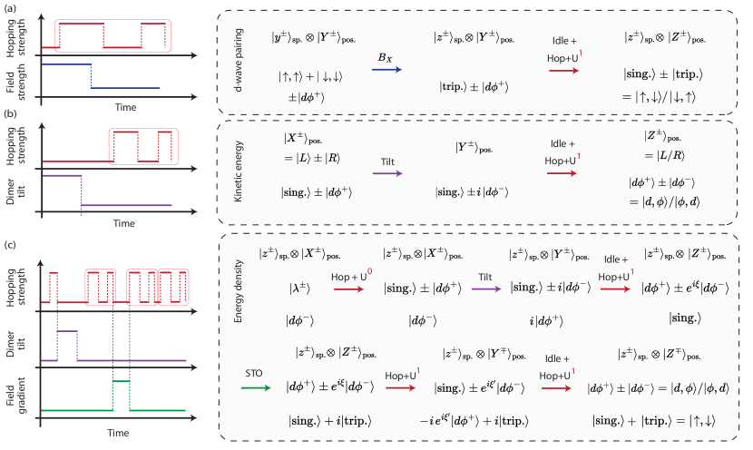
We first develop a protocol to measure the kinetic energy across a dimer. As with the -wave pairing function, we do so by finding a pulse sequence that rotates the eigenvalues of the observable in question (here, the kinetic energy operator) into the readout basis. Like all other observables accessible by this protocol, the kinetic energy operator preserves particle number, and hence can be analyzed in the different particle number sectors. As it turns out, the 1-p sector will pose the bigger challenge than the 2-p sector.
Across a pair of nearest-neighbor sites , the kinetic energy operator on that bond is:
| (94) |
Since this observable is spin-invariant, magnetic field controls are not required. Instead, in addition to particle-hopping control, we also use dimer tilt introduced in Appendix E. As illustrated in Fig. S5(b), our pulse sequence comprises of a -rotation using dimer tilt, followed by the same hopping pulse sequence Hop+U1 that we develop for the -wave pairing measurement in Appendix B.
We look for an appropriate sequence of control parameters that map the eigenstates of into readout basis states. In the 1-p and 2-p sectors, these eigenstates are:
| (95) | |||
| (96) |
where we have omitted the spin degree of freedom on the 1-p eigenstates. These 1-p eigenstates necessitate the use of dimer tilt control. Hopping control performs a rotation about the -axis on the 1-p positional Bloch sphere, and hence the states , as eigenstates of the hopping operator, are invariant. We must first use dimer tilt, which acts as a -axis rotation on the positional Bloch sphere. We perform a rotation to map into , before performing a rotation to map these states to .
However, introducing dimer tilt now complicates the 2-p sector. While hopping and interactions effectively act only on the two-level system spanned by , dimer tilt couples the states. While this complicates our analysis, we use it to our advantage in several ways: (i) by allowing access to the state, we can prepare the superpositions , which are the readout states and , and (ii) by fully transferring population to the state, we can ‘shelve’ information by making them invariant under hopping control. Meanwhile, (iii) the singlet state is invariant under dimer tilt. This greatly simplifies our analysis, simplifying the problem from controlling a generic three-level system to controlling two (coupled) two-level systems one after another.
The pulse sequence acts on the 2-p sector as indicated in the lower row of Fig. S5(b). Beginning from the eigenstates , the dimer tilt coherently transfers population from to . As with the -wave pairing pulse, there is a factor of two difference in the coupling strengths in the 1-p and 2-p sectors, which coincides with the required - vs. -pulses. The initial eigenstates are mapped to . The hopping pulse then coherently maps , which prepares the desired states . The hopping pulse is precisely the same Hop+U1 sequence as the -wave pairing pulse: the parameters and are identical [Eqs. (45-47)], while the initial idling time is slightly modified to match the phases in this pulse:
| (97) | ||||
where we have extended the unitary in Eq. (59) to act on the three-level system .
| (98) |
on the basis , and the unitary is
| (99) |
with the dimer tilt of strength applied for a time . This fully specifies the pulse sequence illustrated in Fig. S5(c).
F.2 Energy density pulse sequence
Having designed a pulse sequence to measure the kinetic energy on a bond , in this section we present a protocol that measures, with a single pulse sequence, the total energy density , given by
| (100) |
where and we have equally divided the interaction energy associated with site among its four adjacent nearest-neighbor bonds on the square lattice. While the energy density on a single dimer can be estimated by separately measuring the kinetic and interaction energies on the dimer, energy-energy correlations between two dimers cannot be estimated in this fashion, since there are kinetic-interaction cross terms which would be missed when we apply global pulses to measure the kinetic and interaction energies. Such energy-energy correlations may be relevant to hydrodynamics experiments, and in the following section we discuss how energy-energy correlations can be used to estimate the temperature of the experimental state.
The primary complicating factor for measuring the energy density is that we have three non-trivial eigenstates of in the 2-p sector, which we want to map to three different readout states with a single pulse sequence while simultaneously achieving the desired mapping in the 1-p sector. The eigenstates and their corresponding target states are:
| (101) | ||||
| (102) | ||||
| (103) |
Note that Eq. (101) is the same in this case as in the kinetic energy measurement, since the interaction energy is only relevant in the 2-p sector. Meanwhile, the states can be mapped to the 2-p eigenstates of the kinetic energy by a simple pulse Hop+U0. However, Eq. (103) is entirely new, since the state has zero kinetic energy but carries interaction energy .
The pulse sequence, illustrated in Fig. S5(c), relies on the kinetic energy pulse sequence as a backbone. Indeed, we first map the eigenstates into the kinetic energy eigenstates , using a hopping pulse sequence which we dub Hop+U0 (details deferred to the end of this section)
| (104) | |||
| (105) |
We then apply the kinetic energy measurement sequence of tilt and hopping pulses discussed in App. F.1:
| (106) | |||
| (107) | |||
| (108) |
The kinetic energy pulse is slightly modified to imprint a phase difference in anticipation of future hopping and idling steps.
The final stage aims to map the singlet state to the readout state . We do so with a magnetic field gradient , which induces singlet-triplet oscillations [74, 75]. This maps , and one can verify that the additional action on the states , which varies between dimers, is irrelevant, since none of our desired information is stored in these states. On the 1-p sector, the field gradient acts as a controlled -rotation, and the states simply acquire complex phases.
| (109) | ||||
| (110) |
We now wish to remove the phase factor in the state . This cannot be achieved with field or field gradient controls, since they are realized by on-site fields and as such cannot change any entanglement, which we need to reach the product state . Indeed, hopping is our only control knob which is capable of generating entanglement. We use two applications of the familiar pulse Hop+U1 to map the part of the state to , idle to remove the phase factor , before mapping back to and giving the readout state . Meanwhile, this process also modifies the relative phase of the superposition. Appropriate choice of in the intermediate step ensures that we arrive at the readout states . In the 1-p sector, this sequence maps to and back into the readout basis . While we could use a pulse that for example, maps at every stage, here we use Hop+U1 since it appears frequently in this work.
| (111) | |||
| (112) | |||
| (113) |
Finally, we provide details on the pulse Hop+U0 that maps the eigenstates . Since we achieve this only with hopping and idling, and the 1-p state remains in , there are no non-trivial matching conditions on this pulse. Here, we design a pulse with the minimal number of steps [Fig. S7(c)]. The idling step takes us to the appropriate tilted arc (this intersection always exists since lies between the tilted axis and the equator, for all values of ), and the hopping step brings us to the equator . The relevant hopping parameters can be solved for by using Eq. (49) and are numerically implemented in the reference code [51].
F.3 Application: thermometry
In this section we discuss a concrete application of the energy-density measurement sequence. Indeed, as discussed above, while the energy density can be estimated by summing the kinetic and interaction energies, estimating energy-energy correlations requires a protocol that directly measures the energy density.
Here we discuss a practical application of such two-point energy correlations: estimating the temperature of a state. Despite its simplicity, estimating the temperature of a Gibbs state in a quantum many-body system remains an open problem. While it is straightforward to estimate the energy of a system, and the average energy is typically a monotonic function of the temperature, one does not know this function a priori, which requires information or assumptions about the density of states (equivalently, the thermodynamic entropy).
With experiments reaching sufficiently low temperatures where numerical simulations no longer serve as a reliable benchmark, developing methods to estimate the temperature of an experiment, in particular with as few assumptions as possible, remains an open problem. Approaches in the literature include coupling the system with a probe system, which suffers from certain fundamental uncertainties [76, 77, 78]. Specific schemes have also been proposed for fermionic quantum gas microscopes [79, 44]. Here, we propose a scheme that can be performed with the pulse sequences we have developed.
We assume that there is an experimental tuning knob which produces Gibbs states of varying temperatures
| (116) |
where is the partition function . Our task is to determine the relation . We do so by noting that the gradient can be estimated by measurements of the average energy and energy variance. By further assuming that we can determine the temperature through other means at a given point (e.g. at sufficiently high temperature through comparison with quantum Monte Carlo methods [80]), knowledge of the gradient allows reconstruction of the curve .
The mean energy and energy variance are related to the temperature by thermodynamic relations. Specifically:
| (117) | ||||
| (118) |
We now apply the chain rule on . We can independently estimate the derivative by measuring at different values of . This gives the estimate of the gradient:
| (119) |
which as discussed above, can be integrated to estimate the curve . The energy variance is simply the sum over all two-point energy correlators between any two dimers :
| (120) |
One can extract almost all of these two-point correlators immediately with the protocol in this work. Below, we comment on two subtleties: dimerization patterns which yield all pairs of bonds that do not overlap, and in the following subsection we sketch a protocol to measure the terms arising from overlapping bonds.
F.3.1 Dimerization patterns
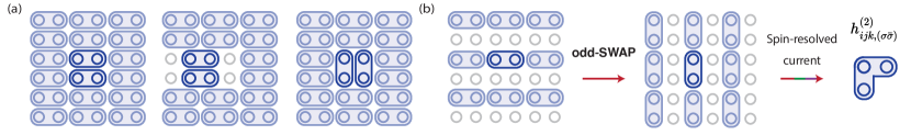
In order to measure all pairs of non-overlapping bonds, we cannot simply use the dimerization pattern in Fig. 1(b). For example, this would only cover some of the possible horizontal-horizontal dimer pairs, even if we could assume translational and rotational invariance. One might guess that some small number of dimerization patterns could yield all dimer pairs. However, any combination of periodic dimerization patterns that could be formed by optical superlattices [36, 37] would not capture all pairs of bonds, given by the least common multiple of the pattern periodicities. For simplicity, we consider a columnar dimerization (Fig. S6(a), left) with periodicity two, and examine horizontal-horizontal dimer pairs on a straight line. This dimerization contains horizontal-horizontal dimer pairs with an even separation. Combining this with a columnar dimerization with periodicity three, for example, would now capture all dimer pairs that are separated by multiples of two or three lattice sites, but would miss every dimer pair with spacings for integer . While this may be sufficient for the purpose of thermometry, where dimer-dimer correlations beyond a certain distance may be ignored, this approach is also experimentally challenging, since it is not straightforward to achieve superlattices of different periodicities.
Instead, we advocate for a different approach. Assuming that we have translational and rotational invariance, we only need three dimerization patterns, illustrated in Fig. S6(a). The first pattern is simply the columnar dimerization. In order to capture the odd-spaced horizontal-horizontal dimer pairs, we then offset a central square by one site (middle). The final pattern involves rotating this central square, which would give all vertical-horizontal dimer pair separations (right). With translational and rotational invariance, this gives us all possible separations between dimer pairs. While the overall dimerization pattern could be performed with an optical lattice, this offset and rotation of the central square would require a certain degree of local control, which could be provided by digital micromirror devices (DMDs) or optical tweezers, which have been recently demonstrated in optical lattice quantum gas microscopes [81, 32].
F.4 Pulse sequences for thermometry: measuring three-body quantities
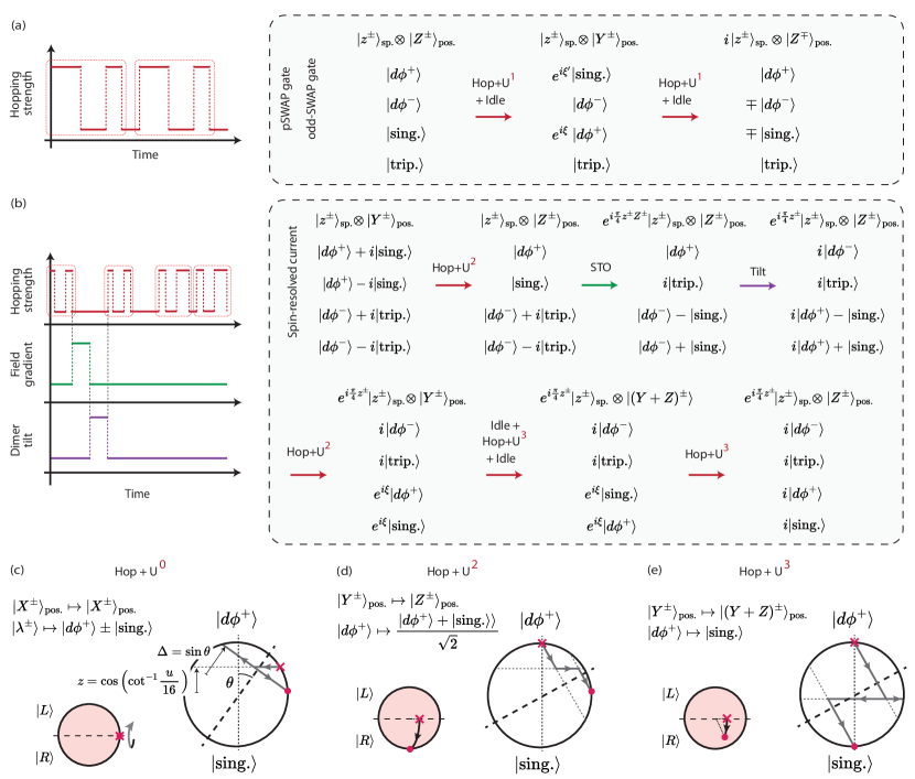
The only bond-bond correlations that cannot be measured with the scheme above are the bonds that overlap. These result in “trimers” of three sites in a straight line or in an ‘L’ shape. Our approach will be the same in either case: we will treat the trimer as two dimers and [Fig. S6(b)]. We first perform operations on , with site isolated, before isolating site and performing operations on dimer . This allows us to use our results on dimer control in this work. However, we note two subtleties: from an experimental point of view, sequentially forming two separate dimers in a coherent fashion may be more challenging to implement than the single-dimerization measurments. From a theoretical point of view, the operations on each dimer should be phase-coherent between multiple particle number sectors, since a number-definite state on the trimer may have indefinite particle number on a dimer. This merely requires us to keep track of the “global phase” of each particle number sector, which we had previously ignored, and requires additional steps in the protocol.
We separate the energy density into kinetic and interaction energy terms. The overlapping terms consist of kinetic-kinetic terms, kinetic-interaction, and interaction-interaction terms. Here, we discuss the kinetic-kinetic terms; the other terms only require nontrivial operations on a single dimer. In turn, these kinetic-kinetic terms comprise products of hopping terms acting on the bonds and of a three-site system and involving either (a) the same spin species or (b) opposite spin species. Our overall strategy will be to apply a pulse on dimer , followed by a pulse on dimer , then measuring all sites .
We develop several pulse sequences to measure the relevant terms. In summary, our proposed strategy is to estimate the kinetic-kinetic terms with: (a) for the same-spin terms, the pSWAP gate on dimer , followed by Hop+U1 on , (b) for opposite-spin terms, the odd-SWAP gate on dimer , followed by applying the spin-resolved current pulse on [Fig. S6(b)]. The kinetic-interaction terms can be estimated with either Hop+U1 on a dimer along with projective readout of the site , or a variant of the spin-resolved current pulse sequence. Finally, the interaction-interaction terms can be directly measured by projective readout. Below, we develop the necessary pulse sequences, which we also summarize in Fig. S7.
F.4.1 Bond-bond correlations with same spin
The terms involving the same spin species are:
| (121) |
To measure this, we could perform a SWAP gate between sites and , and then measure the kinetic energy on dimer . Unfortunately, a SWAP gate, which directly permutes the sites and , is difficult to achieve on all particle-number sectors at once without additional phase factors. Instead, we develop a “pSWAP” gate, which performs the SWAP, along with a phase factor which only depends on the particle-number sector. Concretely, the 1-p, 2-p, and 3-p sectors gain phases of , , and respectively. This will suffice for our purposes, and even be useful, since it is simpler to measure the current [i.e. the eigenstates of ] than the kinetic energy. Having performed the pSWAP, it is simply a matter of measuring the current on (using the Hop+U1 pulse sequence) jointly with the particle density on , and processing the measurements accordingly to obtain the eigenstates of Eq. (121).
The pSWAP gate performs the mapping:
| (122) | ||||
| (123) | ||||
| (124) | ||||
| (125) | ||||
| (126) |
for . The mapping on the 2-p sector is equivalent to
| (127) | ||||
| (128) | ||||
| (129) |
a form which will be helpful for pulse design.
The pSWAP gate simply consists two Hop+U1 pulses, with idling steps interleaved between them [Fig. S7(a)]. On the 1-p and 3-p sectors, this has the effect of performing a pulse, with an overall phase factor of . This phase could potentially be removed by the use of complex-valued hopping strengths [82], but we will not pursue this route here. The 3-p sector will also gain an additional factor of from the interaction term .
On the 2-p sector, each Hop+U1 pulse swaps the states and , and two such pulses return these states to themselves. Interleaving idling times after each Hop+U1 pulse, however, allows one to imprint arbitrary phases and on the and . These pulses have the additional property that the state, which does not otherwise participate in the dynamics, gains the phase . This allows us to engineer the phases and on and respectively. The phase on , which arises solely due to idling, is the same additional phase on the 3-p sector above, and one can verify that the 0-p and 4-p sectors accumulate phase factors of .
F.4.2 Bond-bond correlations with opposite spin
There are two terms involving the opposite spin species, each term being of the form:
| (130) |
where is the opposite spin of . This operator conserves particle number, indeed conserves each spin species separately, and is nontrivial when there are , and and particles on sites and . In the simplest case, the eigenstates and eigenvalues of Eq. (130) are
| (131) | |||
| (132) |
The sector has eigenstates
| (133) | |||
| (134) |
and the eigenstates in the sector are related by exchanging . Finally, the sector has eigenstates
| (135) | |||
| (136) |
In all cases, it is easy to verify the following property: if one performs a SWAP on dimer on the eigenstates (131-136), only when there are an odd number (i.e. 1 or 3) of particles, then in all cases site becomes disentangled from sites . That is, the only non-identity mappings of odd-SWAP are:
| (137) | ||||
| (138) |
Fortunately, this transformation, which we call the odd-SWAP gate, is a simple modification of the pSWAP gate above [Fig. S7(a)], where we instead imprint the phase on all states and . This has the net effect of performing the SWAP along with a phase factor of on both the 1-p and 3-p sectors, while acting as the identity, with phase on the 0-p, 2-p and 4-p sectors.
F.4.3 Pulse sequence to measure spin-resolved current
In fact, after the odd-SWAP gate, the remaining states on have a common property: they are the eigenstates of the spin-resolved current
| (141) |
Specifically, has eigenstates:
| (142) | |||
| (143) | |||
| (144) | |||
| (145) |
In this section, we develop a pulse sequence to measure the spin-resolved current. In addition to its use for estimating the three-body term , one can also verify that a variant of this pulse can be used to estimate the kinetic-interaction energy cross term , where is the anticommutator.
As usual, we seek a pulse on dimer that maps these states into readout states, in the 1-p, 2-p and 3-p sectors. Unlike the pulse sequences on , since we measure immediately after this pulse, we do not have to keep track of the phases on each particle number sector. We design the pulse sequence with the following steps [Fig. S7(b)]:
| (146) | |||
The same pulse sequence also maps the other set of 2-p eigenstates . In the 1-p and 3-p sectors, this pulse sequence realizes the maps
| (147) | ||||
where we have accumulated (spin-dependent) phases which will be irrelevant to the measurement outcomes.
Here, we introduce two new hopping pulse sequences, Hop+U2 and Hop+U3. Hop+U2 is a pulse sequence designed to perform [Fig. S7(d)]: (i) a rotation about the X-axis in the 1-p and 3-p sectors, and (ii) on the 2-p sector, the maps
| (148) | ||||
| (149) |
To design a four-pulse version of this sequence, we follow the analysis of Appendix B.2, and simply use a different starting point , this modifies in Eq. (50) to
| (150) |
where . Matching the coordinates as in Eq. (54) gives the equation
| (151) |
Substituting the 1-p constraint [Eq. (53)] allows to be numerically solved for.
Hop+U3 is a pulse sequence designed to perform [Fig. S7(e)]: (i) a rotation about the X-axis in the 1-p and 3-p sectors, and (ii) the map on the 2-p sector. We perform two Hop+U3 sequences, interleaved by an idling step, to correct for the phase difference accumulated by the previous steps in Eq. (146). This final step also rotates the 1-p and 3-p states into the readout basis. The parameters of Hop+U3 directly follow from the analysis in Appendix B.2, with in Eq. (53) replaced by .
F.4.4 Same-dimer energy correlations
For completeness, we also describe a pulse sequence to measure the energy correlations on the same dimer, i.e. . This introduces a new non-trivial term
| (152) |
This operator is non-trivial only in the 2-p sector, and its eigenstates are precisely the control basis states .
Our approach to map these states into the readout basis will be to exploit dimer tilt and the singlet-triplet oscillation (STO) to admix and . This admixing on is simply the last four steps of our energy-density pulse sequence [Fig. S5(c)], and we simply prepend a STO step to also mix . This pulse sequence has the added effect of measuring the 1-p and 3-p sectors in the computational basis. Finally, there are also kinetic-interaction energy cross-terms on the same dimer. Measuring this quantity requires precisely the same pulse sequence as measuring the spin-resolved current, modified to account for the lack of the factor of .
F.5 Application: converting parity readout to spin- and charge-resolved measurements
As a final application of the techniques we develop, we demonstrate how our pulse sequences can be used to enhance the readout capabilities of quantum gas microscopes. While in this work we had assumed the capability to perform full spin- and charge-resolved readout, many quantum gas microscopes in fact do not have this capability. Instead, they perform parity readout, in which measurements are able to distinguish whether there is one particle on a site (without resolving vs. ), or either zero or two particles. In other words, it measures the parity (odd or even) of the number of particles on the site. This is due to the presence of light-assisted collisions, in which two particles occupying a lattice site collide and are lost [59]. We note that there are experimental techniques to perform full charge- and spin- measurements by applying a spin-dependent potential which separates and particles into different imaging planes [49, 44]. However, here we analyze the more standard parity measurement scheme and discuss how it can be extended using the pulse sequences developed in this work.
Our results are as follows: with only parity-readout and doublon-readout, the pulse sequences as described in the rest of this work are not sufficient to measure -wave pairing or other quantities discussed in this work. However, additional pulse sequences can be performed right before parity-readout, which together emulate full spin- and charge-resolution. Even without doublon-readout, which is more challenging than parity-readout, a large class of observables, including all those considered in this work, can be measured just with parity-readout augmented by the pulses sequences developed here.
The challenge we seek to address is that parity measurements do not give full spin- and charge-resolved information. These measurements provide experimental probabilities of a set of outcomes, and our goal is to infer the probability distribution of every element of the readout basis , where each probability is the population of the relevant state. Being able to recover would emulate full spin- and charge-resolved measurements on a state, at least for the purpose of observables on dimers. Parity measurements on a dimer give four outcomes: , corresponding to the parity on each site. The probability of each outcome is a sum of the probabilities :
| (153) | ||||
| (154) | ||||
| (155) | ||||
| (156) |
i.e. parity readout groups the 16 spin- and charge-resolved readout basis states into four groups, and cannot distinguish between states within a group. Parity measurement can be augmented by selectively removing particles of a certain spin species, as has been demonstrated in Ref. [59]. For example, by first removing the spins and then measuring, we instead obtain the following outcome probabilities
| (157) | ||||
| (158) | ||||
| (159) | ||||
| (160) |
Similar probability relations are obtained when the particles are removed before measuring parity. Finally, the doublons can be directly imaged by first removing all single particles and then specifically measuring for doublons on a site.
| (161) | ||||
| (162) | ||||
| (163) | ||||
| (164) |
This doublon-imaging step is experimentally more challenging. As we shall see, while it is required in principle for full spin- and charge-resolution, in practice it can often be avoided. To summarize, a conventional measurement scheme on a quantum gas microscope is to perform the following measurements:
-
1.
Parity-projection:
-
(a)
measuring the parity of occupation number on each site.
-
(b)
removing particles and measuring site occupation.
-
(c)
removing particles and measuring site occupation.
-
(a)
-
2.
Removing single and particles, then imaging the doublons.
We now analyze what quantities can and cannot be estimated with these measurements. Simply by counting, one might expect that these four sets of measurements of to be sufficient to reconstruct all , since we have a system of sixteen linear equations for sixteen unknown parameters. This is not true, not just because there are normalization constraints which reduce this to a system of just 12 independent equations. To see this, one can re-write Eq. (153-156) as a matrix equation
| (165) |
where is the vector of spin- and charge- resolved probabilities, and where we have separated the columns by total particle number on the dimer for clarity. We can define similar matrix equations for Eq. (157-164) with matrices and combine them into a matrix equation
| (166) |
where represents the measured probabilities. The goal is to infer the probabilities in the standard basis : this is possible if and only if the matrix has a left-inverse such that , the identity matrix. Unfortunately, this is not the case: the matrix has a five-dimensional null space (i.e. such that when ), which implies that a left-inverse cannot exist. The standard-basis probabilities can only be estimated modulo addition in the null space: for any vector in the null space and coefficient , the measured probabilities and are equal, and therefore and are indistinguishable from the measurement outcomes . As an example, an element of the null space of is the vector .
The null space determines what quantities can and cannot be estimated from the measurement outcomes . For any observable which is diagonal in the readout basis, its expectation value is equal to the inner product of with the probabilities :
| (167) |
can be estimated only if the inner products are equal, which is in turn true if and only if is orthogonal to the nullspace .
As an example, in the measurement protocol discussed in Appendix B, estimating the wave pairing correlator corresponds to processing the probabilities by taking its inner product with the vector
| (168) |
One can check that in fact lies in the null space and therefore -wave pairing cannot be estimated using just measurements 1.abc and 2. However, as we will see below, by appending additional pulse sequences before parity measurements, we can enhance readout capabilities to estimate -wave pairing, along with all other observables considered in this work.
Before discussing the pulse-sequence-enhanced measurements, we first briefly comment on the ability to fully resolve spin- and charge- on a single-site vs. on two sites. Measurements 1(abc) suffice to resolve the spin and charge densities on a single site. Here, each measurement has two measurement outcomes, or , and the matrix is
| (169) |
This matrix is invertible, which indicates that measurements 1(abc) suffice to reconstruct all on-site densities. However, the two-site quantities of interest correspond to nearest-neighbor spin- and charge-correlations and cannot be inferred just from on-site densities: these require more measurement settings which we discuss below.
We seek to enhance the capabilities of parity-readout using our pulse sequences. Three sets of additional pulse sequences will suffice to extend parity- and doublon-readout into full spin- and charge-resolved readout. Our approach is to use pulse sequences to permute the readout basis states. Each permutation will result in a new matrix, which when concatenated results in an invertible matrix equation .
Even though our pulse sequences offer a great deal of flexibility, only a few might be useful here. All our pulse sequences are particle-number conserving and equivalent on the 1-p and 3-p sectors. There are 4! total permutations on the 1-/3-p sectors, but the most easily implemented are global spin-flip (microwave) and exchanging sites (SWAP) by hopping. A global spin-flip would not provide any new information, since it merely exchanges the and measurement outcomes. However, a spin-flip on half the sites, with a magnetic field gradient (which can be implemented with a gradient, or a sequence of , and pulses) gives additional information, outlined below. Analogously, swapping sites over all number sectors would simply exchange the and outcomes. However, the odd-SWAP gate allows for a SWAP only on the 1- and 3-p sectors, which gives new information when combined with and measurements. Finally, we can combine these two operations. These three measurements will turn out to extract as much information as possible and additional permutations (for example, arbitrary permutations on the 2-p sector) do not help. In summary, the additional measurements we consider are:
-
3.
Exchanging on every other site with a magnetic field gradient, then
-
(a)
removing spins and measuring parity.
-
(b)
removing spins and measuring parity.
-
(a)
-
4.
Applying odd-SWAP on the dimer [with the hopping and idling pulse in Fig. S7(a)], then
-
(a)
removing spins and measuring parity.
-
(b)
removing spins and measuring parity.
-
(a)
-
5.
Exchanging on every other site and applying odd-SWAP. In this case, it suffices to only
-
(a)
remove spins and measure parity.
-
(a)
These result in matrices . For example, measurement 3(a) results in the matrix
| (170) |
Each of the five additional steps reduces the dimension of the nullspace by one, and hence the matrix , in which all matrices are concatenated, has no null-space. Therefore, measurements 1-5 together suffice to reconstruct all , mimicking full spin- and charge-resolved readout. In turn, our universality result implies that this enables the expectation values of any number-conserving observable to be measured with the protocol in this work.
Finally, we remark on the role of the doublon-occupation measurement (measurement 2). While it is necessary to completely reconstruct , in many cases the information it provides is not necessary for the quantity in question: indeed, in all applications considered here it is not required. Without measurement 2 (i.e. only measurements 1,3,4, and 5), the concatenated matrix has a one-dimensional nullspace: the vector
| (171) |
Any (diagonal) observable which is orthogonal to can be measured without doublon readout, i.e. by a combination of pulse sequences and parity measurements. This is the case for all observables considered in this work. In addition to the -wave pairing correlator, the kinetic energy (94), energy density (100), and spin-resolved current (146) have data-processing vectors
| (172) | ||||
| (173) | ||||
| (174) |
with . It is easy to verify that all three vectors are orthogonal to above, hence can be estimated only by a combination of pulse sequences and parity readout.
In fact, any of the below conditions are sufficient for an observable to have a data-processing vector that is orthogonal to :
-
(i)
The observable is symmetric under hole-doublon exchange (e.g. )
-
(ii)
The observable has trace zero within each particle sector (e.g. and )
-
(iii)
The observable has trace within each particle sector which is orthogonal to the vector [e.g. has traces ]. Note that (i) and (ii) are special cases of this condition, which is both necessary and sufficient for orthogonality to .
We conclude that a large class of observables can be estimated without the doublon-readout measurement. A simple example of an observable which does require doublon-readout measurements is the density of doublons, which has traces . Finally, we remark that since is proportional to the identity on each particle-number sector, any further number-preserving operations will leave the sum invariant, and hence not add additional information. Therefore, doublon measurement (measurement 2) cannot be replaced by further pulse sequences followed by parity measurement, and we expect doublon measurement to be essential to fully reconstruct .