A Pipeline and NIR-Enhanced Dataset for Parking Lot Segmentation

Abstract

Discussions of minimum parking requirement policies often include maps of parking lots, which are time-consuming to construct manually. Open-source datasets for such parking lots are scarce, particularly for US cities. This paper introduces the idea of using Near-Infrared (NIR) channels as input and several post-processing techniques to improve the prediction of off-street surface parking lots using satellite imagery. We constructed two datasets with 12,617 image-mask pairs each: one with 3-channel (RGB) and another with 4-channel (RGB + NIR). The datasets were used to train five deep learning models (OneFormer, Mask2Former, SegFormer, DeepLabV3, and FCN) for semantic segmentation, classifying images to differentiate between parking and non-parking pixels. Our results demonstrate that the NIR channel improved accuracy because parking lots are often surrounded by grass—even though the NIR channel needed to be upsampled from a lower resolution. Post-processing including eliminating erroneous “holes,” simplifying edges, and removing road and building footprints further improved the accuracy. Best model, OneFormer trained on 4-channel input and paired with post-processing techniques achieves a mean Intersection over Union (mIoU) of 84.9% and a pixel-wise accuracy of 96.3%.

1 Introduction

During the 20th century, nearly all US municipalities came to impose “minimum parking requirements” (MPRs) on new construction: mandates to provide parking in some proportion to the amount of floorspace or number of housing units proposed [14]. Over the last twenty years, amid criticism that these requirements are harmful and based on faulty methodologies  [33, 29], dozens of cities and several states have repealed or substantially liberalized their MPR’s [26]. Discussions of MPRs often involve estimates of how many parking spaces there are and how much land is devoted to parking [16, 8, 19]. Nationally, it is estimated that between 0.64% and 0.9% of US land area (between 722 and 2010 million spaces) is parking [9].

In addition to these statistics, discussions of parking policy in media and legislatures have sometimes involved maps showing parking lots—that is, the outlines of off-street parking lots (See Figure 1(a)). Recently, a US-based group called the Parking Reform Network has released interactive maps with parking lots drawn for the downtown areas of dozens of US cities. Such maps often draw significant attention in media wherever MPRs or other policies are being debated [13, 17, 23, 30, 15]. However, the labor-intensive nature of manually creating these annotations has resulted in limited coverage, typically comprising only downtown areas of select cities. While the companies EarthDefine [12] and SafeGraph [32] sell datasets of parking lot annotations, there is a shortage of open-source datasets.

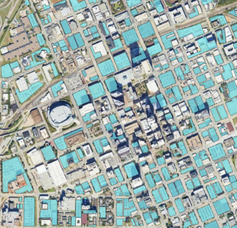
(a) Tulsa, OK

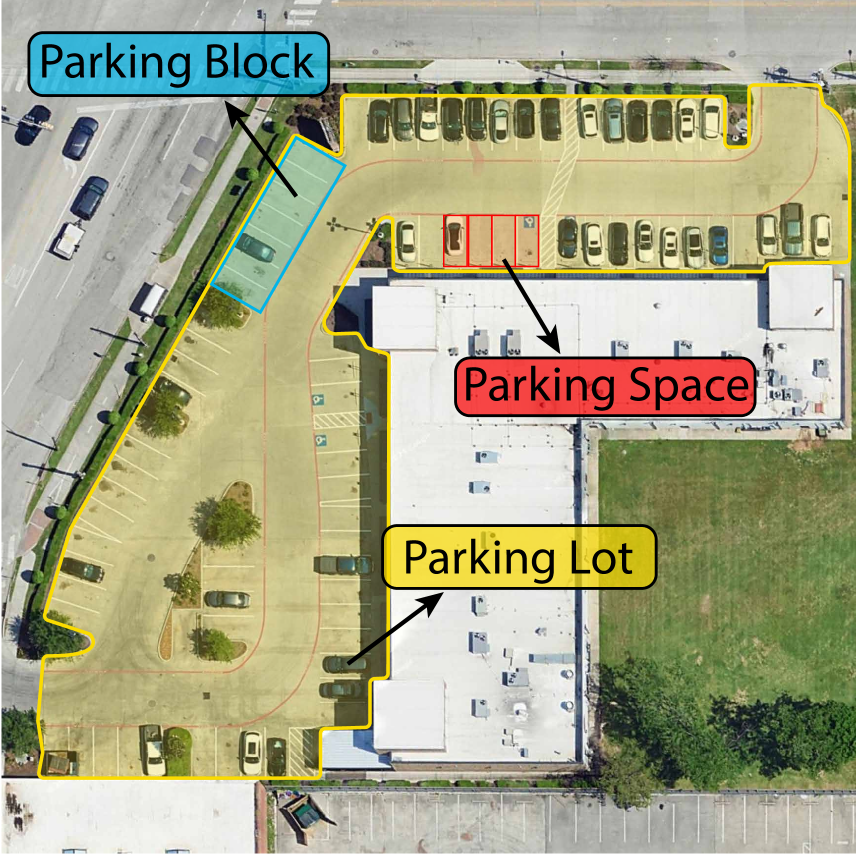
(b) Annotation types

Figure 1: Examples of parking lot annotations

This paper addresses the difficulty of constructing parking lot annotations for large areas. To this end, the following are the paper’s main contributions:

• An open-source dataset consisting of 12,617 satellite image/mask pairs of 512 x 512 dimensions. These masks outline $\sim$35,000 parking lots from 45 US cities.

• We employ five deep learning models (both CNN-based and vision transformer-based) for detecting parking lots using semantic segmentation on satellite images.

• We demonstrate that using images with Near-Infrared (NIR) channels (in addition to RGB) improves segmentation accuracy.

• We propose a post-processing pipeline that improves predictions by removing holes, simplifying edges, and utilizing publicly-available datasets to correct misclassified buildings and roads. These techniques further improve accuracy.

2 Related Work

Segmenting parking lots should be distinguished from other parking-related computer vision tasks that have received more attention in the literature. For example, [2, 1, 20, 37] focus on measuring parking occupancy (i.e., whether spaces hold parked cars) by drawing bounding boxes around parking spaces or parking blocks [21, 34] and then identifying parked cars. These tasks fall under object detection, whereas our approach employs semantic segmentation to detect the entire parking lot (see figure 1(b) for distinctions between parking lots, spaces, and “blocks”). Yin et al. [36] is the only work that attempts to segment parking lots. While that study also utilizes contextual features such as roads, and buildings as input in the deep-learning model, we instead utilize such features in post-processing. Moreover, their dataset consists of 1,344 images in Singapore, whereas ours consists of 12,617 images from the United States.

As [36] point out, segmenting parking lots poses unique challenges: (i) variation in size and shape of parking lots; (ii) overlap with other objects such as vehicles and vegetation. In addition, since our goal is to segment parking lots across the United States, we also face (iii) substantial differences among cities in foliage, paving materials, sidewalk designs, and other factors.

Table 1 provides a summary of other datasets that are related to detecting parking lots.

Dataset	Annotations	# Images	View	Open-Source	NIR channel
Safe Graph [32]	Parking Lot	NA	Satellite	✗	✗
Earth Define [12]	Parking Lot	NA	Satellite	✗	✗
Grab-Pklot [36]	Parking Lot	1,344	Satellite	✓	✗
ParkSeg, Ours	Parking Lot	12,617	Satellite	✓	✓

Table 1: Comparison of datasets.

3 Dataset Construction

This section describes the construction of the dataset, which consists of:

• 297.7 $\mathrm{k}\mathrm{m}^{2}$ of total area

• 62.5 $\mathrm{k}\mathrm{m}^{2}$ of labeled parking area

• 35,127 annotated parking boundaries.

• 12,617 PNG image-mask pairs

3.1 Parking Lot Annotations

The first step in constructing the training dataset is to produce parking lot annotations. To produce these, we started out with two data sources:

• Parking Reform Network (PRN) data: parking lots located in the downtown areas of 42 US cities. For most cities, this consists of the areas within the innermost beltway of freeways. These were created by the Parking Reform Network (PRN) for their interactive maps.

• OpenStreetMap (OSM) data downloaded for the entirety of three cities: Champaign IL, Anaheim CA, and Lubbock, TX. These cities were selected because they are in different parts of the country.

Both datasets required substantial modification for the purpose of training. As [36] notes, the OpenStreetMap (OSM) dataset contains many mistakes. More fundamentally, neither dataset was created to train a model for semantic segmentation, which mattered in three primary ways:

1. Garages: Our dataset only includes parking garages with parking lots visibly on top of them. The model cannot visually distinguish the purpose of a building.

2. Boundaries: Parking lot annotations must be drawn along the edge of the pavement, in order for the deep learning model to learn visual cues. See Figure 2 for an example. Within OSM, the annotations run along the edge of the parcel rather than the parking lot itself.

3. Outdated: Annotations within OSM are not up-to-date at times and therefore are out-of-sync with the latest satellite images. See Figure 3 for example, where the parking lot edges are drawn with reference to a building that no longer exists.

(a) OSM Annotation

(b) Corrected Annotation

Figure 2: Corrected example with annotations drawn along pavement edge

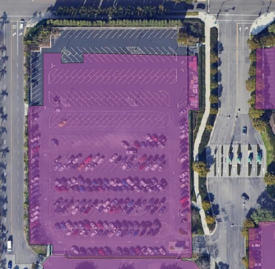
(a) OSM Annotation

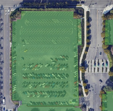
(b) Corrected Annotation

Figure 3: Corrected example where OSM annotation is out-of-sync with satellite image

In addition, for the 42 cities with PRN data, we expanded the dataset by adding several parking lots outside the downtown areas that PRN originally labeled.

To correct and expand the datasets, a team of students refined the data in the QGIS app by overlaying the polygons over a Google Satellite basemap. The correction process involved removing incorrect polygons that are no longer parking areas, adding missing parking polygons, and aligning the parking lots’ edges to the Google basemap we are using. In the end, this process yielded the corrected annotations, which are exported from the QGIS app and partitioned into non-overlapping PNG images of 512x512 pixels. These label images (masks) are single-channel images with pixel values of ‘0’ for the background and ‘1’ for the parking areas.

Note that in drawing annotations, there are inevitably judgement calls about what “counts” as parking. If a driveway leads to a parking lot, is that part of the parking? Or is it a private road which provides vehicle access from the street to a door that opens into the parking lot? For driveways, we have allowed students to rely on case-by-case judgement and encouraged them to incorporate only very short driveways—in order to keep the model from learning to recognize roads generally. Similarly, consider our decision to end parking at the edge of the pavement surface rather than the edge of a parcel. In understanding certain impacts of parking, it may be sensible to consider entire parcels when they are primarily used for parking. For example, if the parcel in Figure 2 were not devoted to parking, then perhaps it could be a residential parcel yielding a certain expected property tax per acre. Different definitions may be better for some purposes than others.

3.2 RGB Satellite Tiles

After the annotation masks were created, for basemap, we exported the Google Map tiles from QGIS to PNG files with a resolution of 30 cm per pixel, a size of 512x512 pixels each and three Red/Green/Blue color channels. Figure 4 shows an example image and its parking lot mask. There are no images in the dataset without parking areas. On average, 21% of each image is covered by parking pixels.

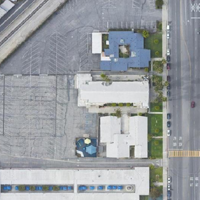
(a) Image

(b) Mask

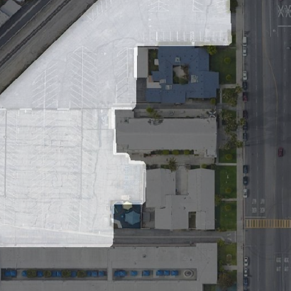
(c) Mask and Image

Figure 4: An example of a 512x512 pixels image and its annotation mask in our dataset

3.3 Enriching tiles with near-infrared

The National Agriculture Imagery Program (NAIP) provides a tile set of aerial imagery for the United States which has four color channels: Red, Green, Blue, and Near Infrared (NIR). Figure 5 shows some examples of this imagery, displayed with the true Red channel swapped for the NIR channel. Vegetation reflects more NIR, so the grass and foliage around the border of the parking lots stand out. We hypothesized that this contrast could aid the model in detecting edges, since many parking lots are surrounded by grass.

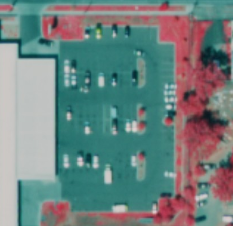
(a)

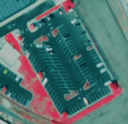
(b)

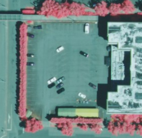
(c)

Figure 5: Examples of NAIP imagery

A drawback to the NAIP dataset is that it has a resolution as low as 1 m/pixel in some areas, whereas the Google satellite imagery has 30 cm/pixel. Therefore, we created a second training dataset of 30 cm/pixel tiles which combine the Red/Green/Blue channels from Google Maps with a “resampled” NIR channel exported from NAIP tiles. To convert the NIR channel to 30 cm/pixel, it is necessary to apply raster resampling, which fill in missing pixel values. For resampling, we use bilinear interpolation, which takes a weighted average of the four nearest pixels in the original image to determine the value of each missing pixel (see [24]).

As a result, the dataset contains of two sets of 12,617 image-mask pairs: one set includes 3-channel images, and the other set 4-channel images. Both sets have a 30 cm/pixel resolution and are 512x512 pixels.

4 Method

This section describes the experimental procedure, including the deep learning models and the post-processing steps implemented to improve the accuracy of the results. Figure 6 shows the overall workflow, which is divided into two phases: training and inference. The training phase comprises two parts of data construction and model training. The inference phase includes obtaining predictions from the deep learning model and performing post-processing on the results.

Figure 6: Workflow Diagram

4.1 Deep Learning Models

We tackle the parking lot segmentation problem using semantic segmentation: a core task in computer vision where each pixel in an image is classified into a predefined category. In our case, the task involves binary classification: identifying pixels as either “parking” or “not parking.” Today, Convolutional Neural Networks (CNNs) and vision transformers are two prevalent methods used for this task. Below, we test five models: two CNN-based, including Fully Convolutional Networks (FCNs) [27] and DeepLabV3 [5], and three transformer-based, including SegFormer [35], Mask2Former [6], and OneFormer [22].

We utilize the models with their original architecture. Therefore, we do not delve into the architectures and layers here. The only modifications we make are to the first layer (when using 4-channel images as input) and the last layer, since we have only one class in addition to the background. The rest remains the same as in their original papers. The following sections will explain some key features of each model, and the pretrained weights we used for each one.

4.1.1 FCN

Fully Convolutional Neural Networks (FCNs) [27] was the first architecture to convert classification-based CNNs into fully convolutional models that predict dense output for every pixel. This feature helps them to maintain spatial hierarchies throughout the network, allowing them to handle arbitrary input image sizes.

4.1.2 DeepLabV3

DeepLabV3 [5], an extension of the original DeepLab model [4], designed to address the challenge of capturing multi-scale contextual information in CNN-based approaches. By incorporating atrous (dilated) convolutions and the Atrous Spatial Pyramid Pooling (ASPP) module, DeepLabV3 effectively expands its receptive field and aggregates multi-scale features without increasing computational costs.

4.1.3 SegFormer

SegFormer [35] is a novel deep learning model that combines the strengths of CNNs and transformers to segment images. Transformers, originally designed for natural language processing tasks, are capable of capturing long-range dependencies and contextual information. By combining this ability with the robust spatial feature extraction of CNNs, SegFormer excels in understanding both local details and global context.

4.1.4 Mask2Former

Mask2Former [6] adopts the same universal architecture as MaskFormer [7] but uses masked-attention instead of standard cross-attention used in transformer-based architectures. Masked attention only attends to the foreground region of the predicted mask for each query, which leads to a faster convergence and performance. They also implement multi-scale high-resolution features to handle small objects or regions. Unlike previous universal architectures, Mask2Former outperforms specialized architectures trained on specific tasks such as semantic or instance segmentation.

4.1.5 OneFormer

OneFormer [22] is built on the idea to have a universal architecture and model for semantic, instance and panoptic segmentation tasks. Unlike Mask2Former, Oneformer does not require training on each task individually — by employing a task-conditioned joint training strategy. They compute a query-text contrastive loss which helps the model learn inter-task distinctions. However, since our interest is semantic segmentation alone, we do not use contrastive loss while fine-tuning the model.

4.1.6 Training Setup

The training and validation sets are randomly partitioned, with a 90%-10% ratio. The test set, however, consists of 400 images from a different city that was not included in the training or validation phases (in addition to the 12,617 images mentioned).

All five models were implemented in Python using the PyTorch library [31], and the experiments were conducted on an NVIDIA RTX A4000 GPU with 16 GB of memory and an Intel Xeon CPU.

Regarding hyperparameters, the learning rate is set to 1e-5, and the Adam optimizer is utilized. We also use an early stopping method to halt the model once it converged. This method had a patience value of 10 epochs.

To optimize model performance, we need a loss function that quantifies model’s errors during the training process. Since our problem involves binary classification for each pixel (“parking” or “not parking”), we use Binary Cross Entropy (BCE) with Logits Loss, which combines a Sigmoid layer and BCE loss [3]. Equation 1 shows the loss function:

$$\small L=\frac{1}{N}\sum_{n}\left[-w_{n}\left(y_{n}\cdot\log\sigma(x_{n})+(1-y_{n})\cdot\log(1-\sigma(x_{n}))\right)\right],$$ (1)

where $L$ is the loss value, $N$ is the batch size, $w_{n}$ is a weight for positive class, $y_{n}$ is the true label of sample $n$, $x_{n}$ is the input feature of sample $n$, and $\sigma$ denotes the sigmoid function.

Since the proportions of background and parking lots in the images are significantly different (on average, 21% parking and 79% background), we have an imbalanced class situation. Therefore, we use $w_{n}=\frac{1}{0.21}$ as the positive weight in the loss function. This assigns a factor of 4.76 to the parking labels (positive class) and 1 to the background, prioritizing the correct prediction of parking lot pixels over background pixels.

Model performance is evaluated using two commonly-used metrics:

• Pixel-wise accuracy (PW): Pixel-wise accuracy measures the percentage of pixels that are correctly predicted as either background or parking lot.

• mean Intersection over Union (mIoU): This metric evaluates the average IoU for all classes (including background), measuring the overlap between the predicted mask and the ground truth mask:

  $$IoU(A,B)=\frac{|A\cap B|}{|A\cup B|}$$ (2)

  where $|A\cap B|$ is the area of overlap (intersection) between the predicted and ground truth masks, and $|A\cup B|$ is the area of union between the predicted and ground truth masks. This metric is computed for all the classes and the average is called mIoU.

4.2 Post-Processing

Our post-processing stage modifies the outputs of the deep learning models, in order to obtain edges that are simpler and more accurate. To do so, we first convert the prediction masks into a single GeoJSON file containing the predicted parking polygons. Since we know the geographic bounding box of every image in the test dataset, it is straightforward to map every pixel in each test to a latitude/longitude pair. After doing so, we render all the predicted parking lot annotations as geometry polygons in a single, large GeoJSON file. Once the GeoJSON file is created, we carry out our post-processing tasks by modifying the polygons. These tasks include (i) removing small “holes”, (ii) simplifying boundary edges, (iii) removing areas which are actually buildings, and (iv) removing areas which are roads. The following sections explain each task in more detail.

4.2.1 Removing Holes

The deep learning models often output masks with small “holes,” which are nearly always incorrect. There are two kinds of holes. Figure 7(a) shows a hole (outlined in blue) which is a small, erroneous gap in the parking lot mask. Figure 7(b) shows holes (in pink) which are small masks themselves. Manual inspection revealed that nearly all such holes are errors in output. While parking lots vary in size and sometimes have “islands” within them, it is apparently the case that, the smaller the hole, the more likely it is to be an error. Therefore, we hypothesized that eliminating holes smaller than a defined threshold would improve the model’s accuracy. By trial-and-error, we chose 60 $m^{2}$ as the threshold.

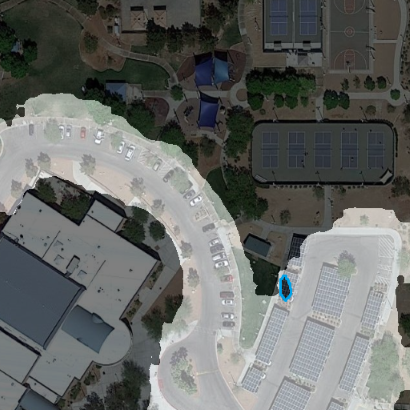
(a) Example of gap in the mask

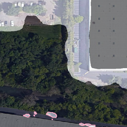
(b) Example of mask holes

Figure 7: An example polygon before and after removing holes

4.2.2 Simplifying Edges

Rough and complex edges are another common issue in segmentation output. Figure 7 also illustrates this problem. Rough edges often indicate inaccurate predictions, because parking lots have relatively simple edges. Rough edges also make it more difficult for someone to manually correct the model output later, since the resulting polygons have more vertices to fix.

Thus, our next post-processing step is to simplify the parking lot edges. To do so, we use Mapshaper [18]: a tool for editing Shapefile, GeoJSON, and raster data formats. We use the tool to apply the the Douglas-Peucker algorithm for shape simplification [11]. The goal of this algorithm is to reduce the total number of points composing a line or curve while maintaining a similar shape. We implement this algorithm in Python by setting a maximum percentage of points that can be removed. Figure 8 shows an example of a parking lot annotation, along with the vertices before and after simplification. The simplified polygon classifies fewer non-parking pixels as parking. It is also much easier to correct manually in GIS software by dragging vertices into place.

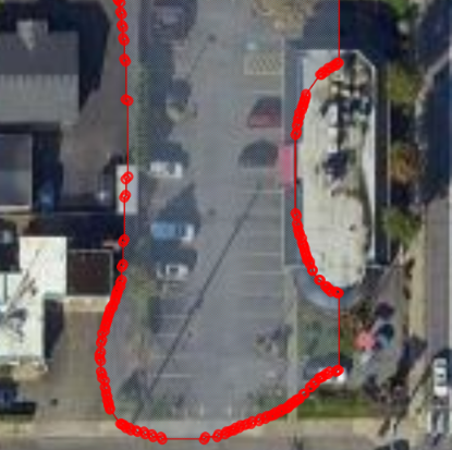
(a) Before simplification

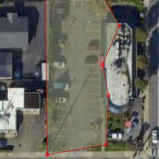
(b) After simplification

Figure 8: An example polygon before and after simplification

4.2.3 Removing Buildings

Building roofs are similar in color and shape to parking lots. Consequently, the models often misclassify parts of roofs as parking. To address this problem, Yin et al. [36] incorporate extra channels containing building information into their model with success. We instead utilize the open-access “building footprint” dataset provided by Microsoft [28], which provides annotations for all nearly all buildings in the United States. We take the model’s prediction and simply subtract the building footprints using Python’s Shapely library. Figure 9 shows an example of an area before and after building removal.

(a) Before building correction

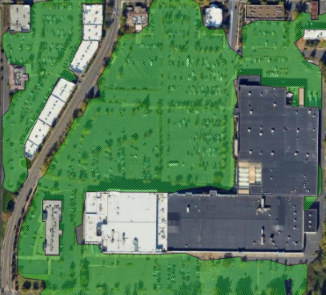
(b) After building correction

Figure 9: An example polygon before and after correcting buildings’ mistakes. The building dataset is displayed in red in (a).

4.2.4 Removing Roads

Roads are the most similar landscape feature to parking lots, so the models sometimes mistake portions of roads for parking. Yin et al. [36] address this challenge by incorporating roadways as additional input channels in training data. For computational simplicity, we incorporate roadway information into post-processing. The road data is sourced from OpenStreetMap, where roads are represented as LineStrings that follow road centerlines. We create buffers around each centerline with widths that vary with the number of lanes recorded for each road. Then, the buffers are subtracted from the predicted parking lot polygons. Figure 10 shows an example.

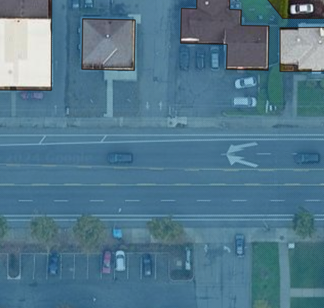
(a) Before road correction

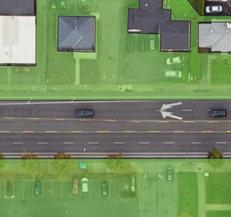
(b) After road correction

Figure 10: An example polygon before and after correcting roads’ mistakes.

Table 2: Performance Comparison of Different Models. Bold indicates the best model for the metric and technique. Box indicates the best model overall for the respective metric

Model	Backbone	Pre-training Dataset	Training Images	Original		w/ Building Removal		w/ Road Removal
				mIoU	PW	mIoU	PW	mIoU	PW
FCN	ResNet50	COCO [25]	RGB	77.92	94.22	79.55	94.54	80.18	94.81
			RGB + NIR	80.18	94.83	82.13	95.43	82.45	95.54
DeepLabV3	ResNet50	COCO [25]	RGB	79.62	94.76	81.56	95.31	81.89	95.43
			RGB + NIR	80.06	94.91	82.32	95.48	82.74	95.63
SegFormer	MiT-B0	ADE20K[38]	RGB	81.47	95.33	82.21	95.59	82.42	95.66
			RGB + NIR	81.75	95.24	83.32	95.79	83.53	95.87
Mask2Former	Swin-L	CityScapes[10]	RGB	82.04	95.22	82.69	95.74	82.99	95.85
			RGB + NIR	82.06	95.23	83.31	95.68	83.92	95.88
OneFormer	Swin-L	COCO [25]	RGB	83.23	95.72	84.55	96.15	84.73	96.21
			RGB + NIR	$\mathbf{84.05}$	$\mathbf{96.07}$	$\mathbf{84.59}$	$\mathbf{96.26}$	$\mathbf{84.86}$	$\mathbf{96.34}$

5 Results and Analysis

This section presents the results of the five deep learning models, both before and after our post-processing steps. Table 2 shows the accuracy results. Since the first two post-processing tasks—removing holes and simplifying edges—have minimal individual effects, they are evaluated jointly along with the building removal task. The results for this combined evaluation are reported under the category “w/ Building Removal.” Moreover, to simplify comparisons given the numerous metrics, the post-processing results are cumulative: for example the “w/ Road Correction” results are calculated based on the “w/ Building” output. The best performance was achieved using the OneFormer model trained by 4-channel images after post processing, with an mIoU of 84.4% and pixel-wise accuracy of 96.2%. More discussion of the results and examples appear below.

5.1 Model Comparison

Table 2 shows OneFormer significantly outperforms the other models on both metrics. OneFormer achieves approximately an 5.3% increase in the mIoU metric compared to FCN for the model trained with RGB images and an 3.9% increase when the NIR channel is included. The table is organized by performance, from FCN to OneFormer, with higher-performing models listed later. SegFormer also shows an improvement, with a 3.6% higher mIoU for RGB-trained models compared to FCN. This improvement is particularly notable given that SegFormer has only 3.7 million parameters compared to FCN’s 49.6 million. The same situation holds when comparing DeepLabV3 and SegFormer. Overall, models leveraging vision transformers demonstrated better performance than both DeepLabV3 and FCN.

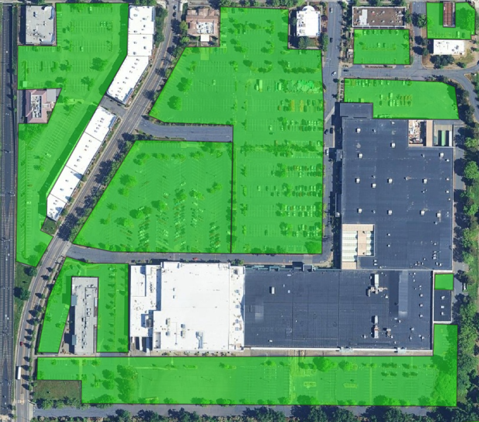
(a) Ground Truth

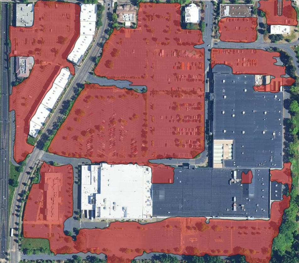
(b) FCN

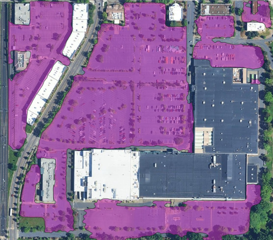
(c) DeepLabV3

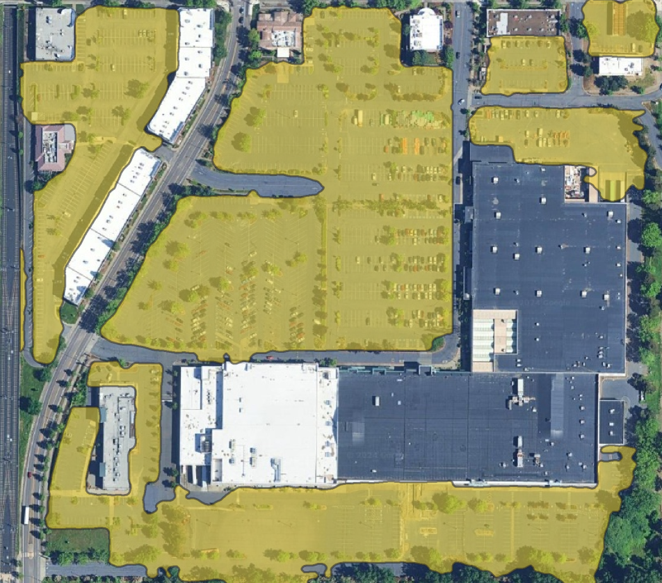
(d) Segformer

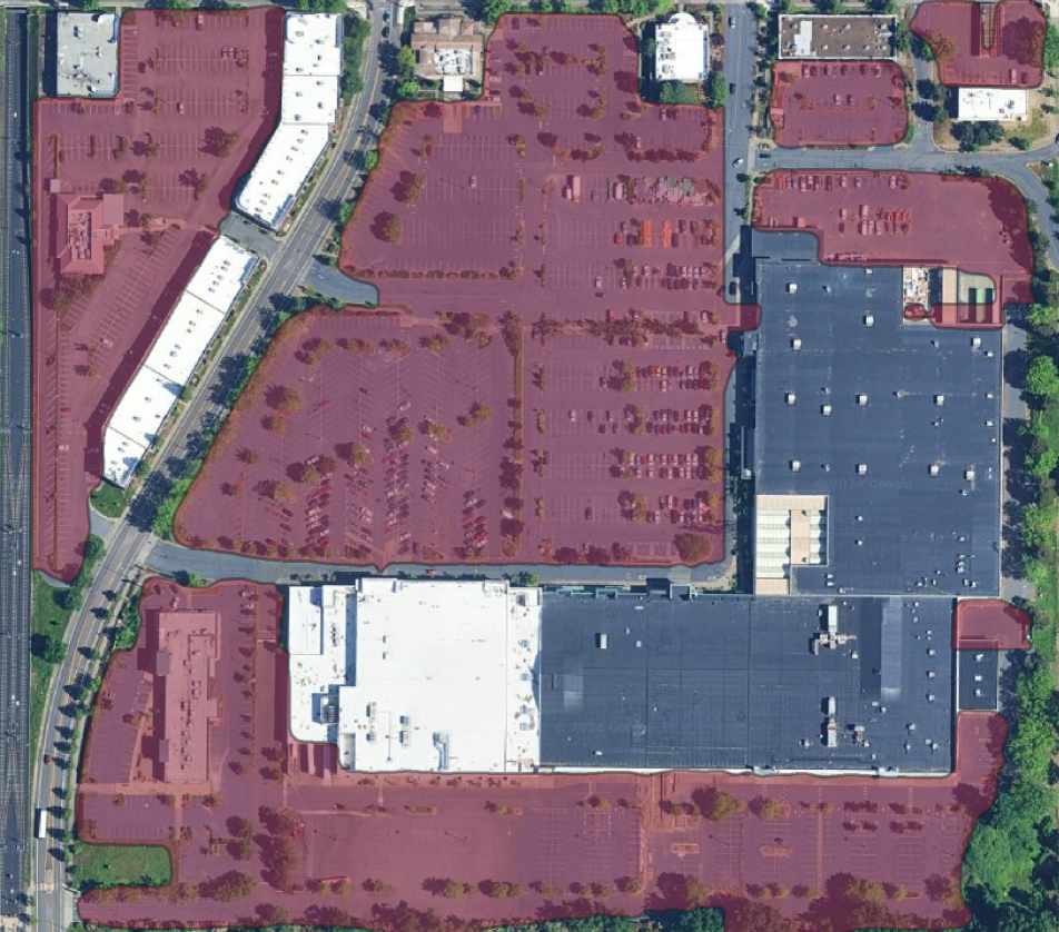
(e) Mask2Former

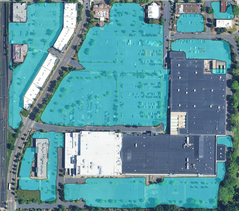
(f) Oneformer

Figure 11: Comparison between different models across a test area. The colored polygons indicate the true parking areas in (a), and the predictions in the remaining subfigures. The predictions are from models trained with RGB+NIR images and shown before post-processing.

Figure 11 provides a visual comparison of model performance, with subfigure (a) showing the ”ground truth” and subfigures (b) through (f) displaying predictions from five different models for an example area of the test dataset. In this case, all models shown are only trained on RGB channels. (NIR enrichment is discussed below.) While all models demonstrate acceptable performance, DeepLabV3 and FCN tend to overpredict parking lot areas, mistakenly classifying non-parking pixels, such as parts of buildings or roads, as parking. In contrast, the predictions from the other models more closely align with the ground truth. Although post-processing tasks correct some of these errors, challenges in accurately detecting edges limits the overall accuracy for the first two models.

5.2 Impact of Near-Infrared Channel

Table 2 shows that incorporating the NIR channel improved all models’ accuracy. This improvement is most pronounced in FCN, with a 1.3% increase in mIoU, compared to the other models. This suggests that the NIR channel has the most benefits when the model’s baseline performance is lower.

Figure 12 shows five examples in which the NIR channel improves models performance. In this figure, we overlay the predictions of two models (one trained with RGB images and the other with RGB+NIR images) to better highlight the differences. It is clear that model with NIR detects edges better and overpredicts parking less often. In particular, the NIR channel keeps the model from erroneously merging nearby parking lots together, as seen in subfigures (a), (b), and (e). Reasonably, this happens because the NIR channel makes the grassy areas between nearby parking lots stand out more clearly. In subfigures (a) and (c) it aided in distinguishing buildings from parking lots, and in subfigure (a), it ensured the entire parking lot is recognized without missing any sections. Across all examples, the NIR channel consistently mitigates overprediction issues.

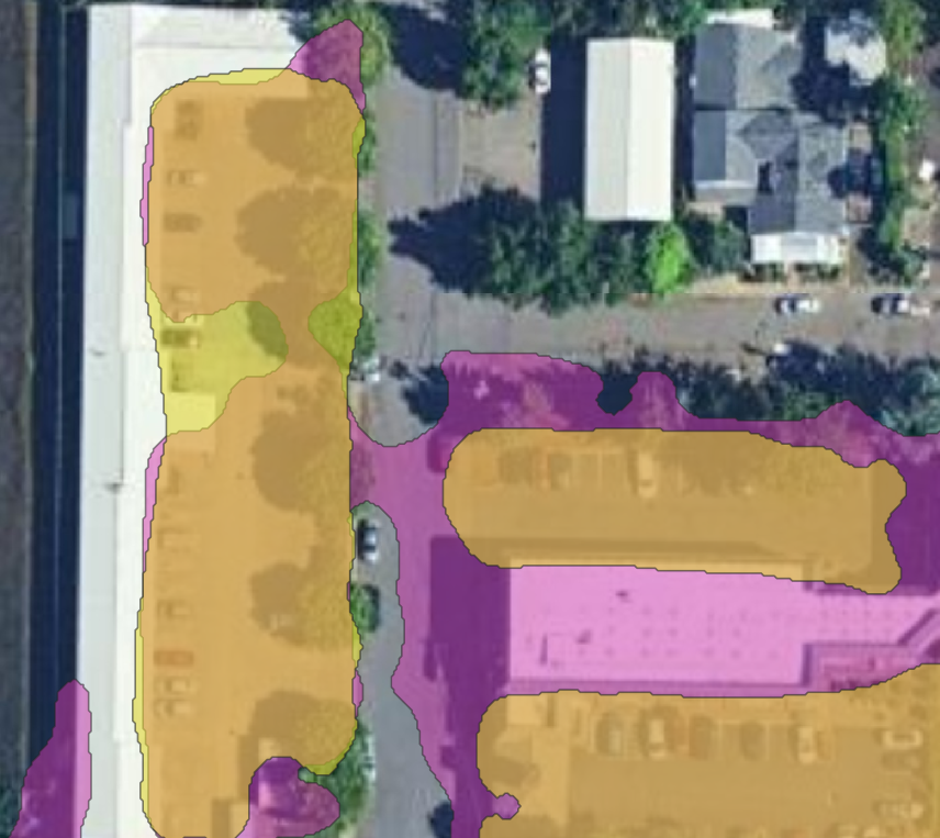
(a) FCN

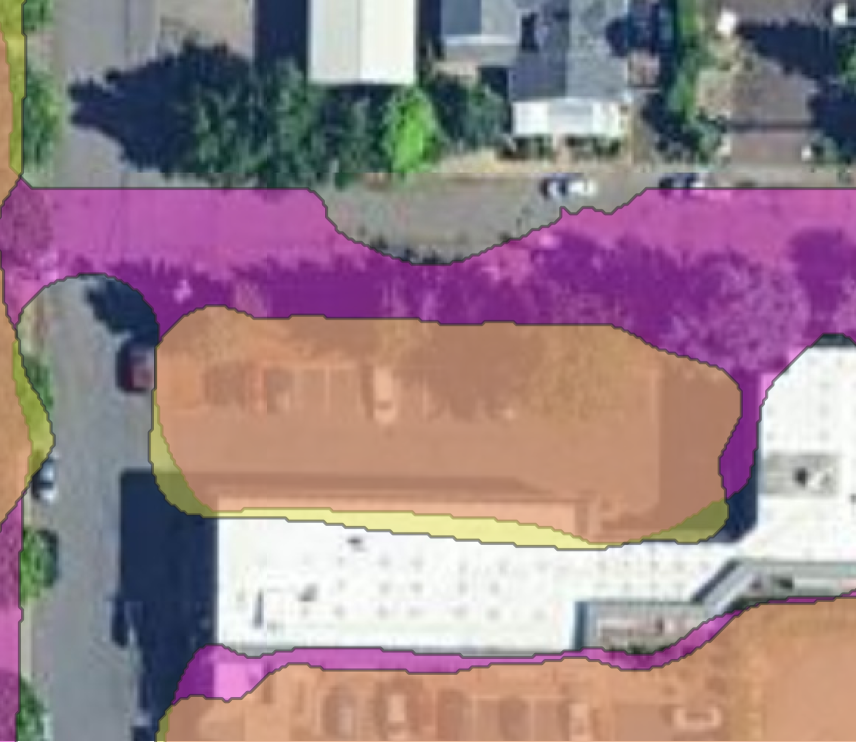
(b) DeepLabV3

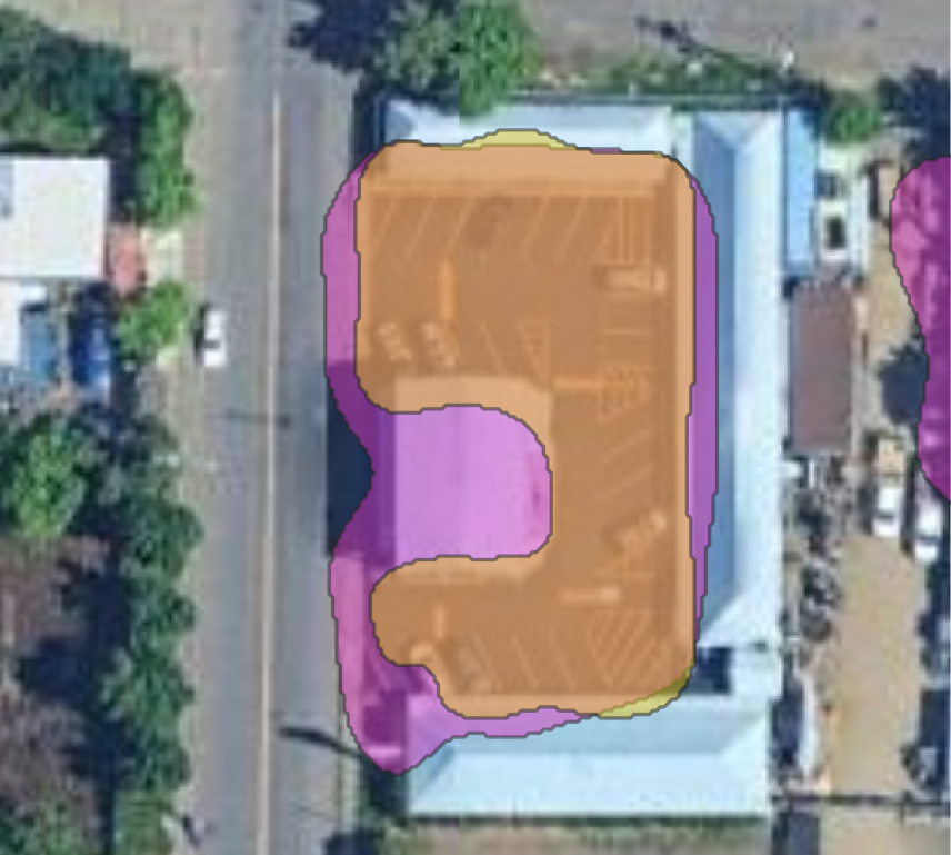
(c) SegFormer

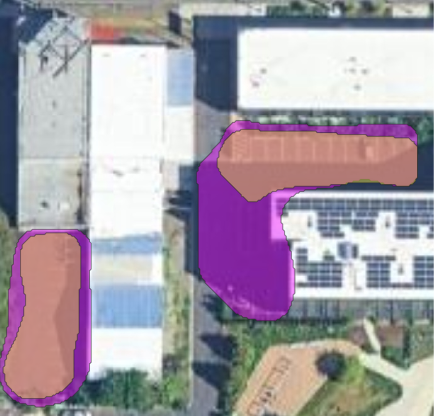
(d) Mask2Former

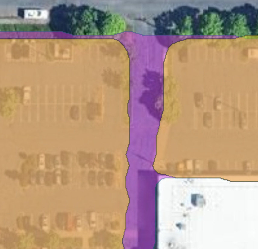
(e) OneFormer

Figure 12: Examples of impact of adding the NIR channel: Purple polygons show RGB model predictions; yellow shows RGB+NIR. The predictions are shown before post-processing.

5.3 Impact of Post-processing

We analyze post-processing in two stages: building removal (which includes removing holes, smoothing edges, and correcting misclassified building polygons) and road removal. Table 2 shows that building removal improved the models’ mIoU accuracy by an average of 1.38% and pixel-wise accuracy by 0.55%, with a more pronounced effect in DeepLabV3 (2.1% in mIoU) and FCN (1.8% in mIoU). SegFormer, Mask2Former, and OneFormer saw smaller but still meaningful gains, given their already high baseline accuracies. The final step, road removal, further improved mIoU by 0.35% and pixel-wise accuracy by 0.12%. Despite their computational efficiency, these post-processing steps yield notable improvements, enhancing the overall quality of the predictions.

6 Conclusion

This paper introduces a multi-step procedure for predicting parking lot segments from satellite images and producing GeoJSON files that users can easily correct. We constructed a dataset of two sets of 12,617 image-mask pairs: one with 3-channel images (RGB) and another with 4-channel images (RGB + Near-Infrared). These images were used to train five deep learning models (OneFormer, Mask2Former, SegFormer, DeepLabV3 and FCN) for image segmentation. Four post-processing steps carried out on the predicted masks were shown to improve model accuracy, as did enriching images with an NIR channel—even though the NIR channel as upsampled to a higher resolution. The best performance was achieved using the OneFormer model trained on 4-channel images with post-processing, with a mIoU of 84.9% and a pixel-wise accuracy of 96.3%.

The fact that an automated process can achieve reasonably high accuracy shows a pathway for deep learning to contribute to current discussion of urban form and public policy. This process—or a similar one—could be used to produce statistics, plots and maps of interest to those considering changes to parking minimums or other laws.

References

- [1] Giuseppe Amato, Fabio Carrara, Fabrizio Falchi, Claudio Gennaro, Carlo Meghini, and Claudio Vairo. Deep learning for decentralized parking lot occupancy detection. Expert Systems with Applications, 72:327–334, Apr. 2017.
- [2] Giuseppe Amato, Fabio Carrara, Fabrizio Falchi, Claudio Gennaro, and Claudio Vairo. Car parking occupancy detection using smart camera networks and Deep Learning. In 2016 IEEE Symposium on Computers and Communication (ISCC), pages 1212–1217, June 2016.
- [3] Christopher M. Bishop and Hugh Bishop. Deep Learning: Foundations and Concepts. Springer International Publishing, Cham, 2024.
- [4] Liang-Chieh Chen, George Papandreou, Iasonas Kokkinos, Kevin Murphy, and Alan L. Yuille. DeepLab: Semantic Image Segmentation with Deep Convolutional Nets, Atrous Convolution, and Fully Connected CRFs. IEEE Transactions on Pattern Analysis and Machine Intelligence, 40(4):834–848, Apr. 2018.
- [5] Liang-Chieh Chen, George Papandreou, Florian Schroff, and Hartwig Adam. Rethinking Atrous Convolution for Semantic Image Segmentation, Dec. 2017.
- [6] Bowen Cheng, Ishan Misra, Alexander G. Schwing, Alexander Kirillov, and Rohit Girdhar. Masked-attention Mask Transformer for Universal Image Segmentation, June 2022.
- [7] Bowen Cheng, Alexander G. Schwing, and Alexander Kirillov. Per-Pixel Classification is Not All You Need for Semantic Segmentation, Oct. 2021.
- [8] Mikhail Chester, Andrew Fraser, Juan Matute, Carolyn Flower, and Ram Pendyala. Parking Infrastructure: A Constraint on or Opportunity for Urban Redevelopment? A Study of Los Angeles County Parking Supply and Growth. Journal of the American Planning Association, 81(4):268–286, Oct. 2015.
- [9] Mikhail Chester, Aprad Horvath, and Samer Madanat. Parking Infrastructure and the Environment. ACCESS Magazine, 1(39):28–33, Oct. 2011.
- [10] Marius Cordts, Mohamed Omran, Sebastian Ramos, Timo Rehfeld, Markus Enzweiler, Rodrigo Benenson, Uwe Franke, Stefan Roth, and Bernt Schiele. The Cityscapes Dataset for Semantic Urban Scene Understanding. In Proceedings of the IEEE Conference on Computer Vision and Pattern Recognition, pages 3213–3223, 2016.
- [11] David H Douglas and Thomas K Peucker. Algorithms for the reduction of the number of points required to represent a digitized line or its caricature. Cartographica: The International Journal for Geographic Information and Geovisualization, 10(2):112–122, Dec. 1973.
- [12] EarthDefine. EarthDefine | US Parking Lots: High-resolution mapping of all large parking spaces in the US. https://www.earthdefine.com/parking/, 2021.
- [13] Josh Fenton. 24% of Downtown Providence Is Parking — Is that Good or Bad. https://www.golocalprov.com/news/24-of-downtown-providence-is-parking-is-that-good-or-bad, Aug. 2023.
- [14] Erik Ferguson. Zoning for Parking as Policy Process: A Historical Review. Transport Reviews, 24(2):177–194, Mar. 2004.
- [15] Cornelius Frolik. Nearly 1/3rd of downtown Dayton is off-street parking. Is that too much? https://www.daytondailynews.com/local/nearly-13rd-of-downtown-dayton-is-off-street-parking-is-that-too-much/SG7TKJASAFFQRGFTVUDXUVF5NE/, Feb. 2024.
- [16] C.J. Gabbe, Taner Osman, and Michael Manville. The opportunity cost of parking requirements: Would Silicon Valley be richer if its parking requirements were lower? Journal of Transport and Land Use, 14(1):277–301, 2021.
- [17] Heather Gann. 26% of land in downtown Birmingham is dedicated to parking. Is that space being wasted? https://www.al.com/news/2023/08/26-of-land-in-downtown-birmingham-is-dedicated-to-parking-is-that-space-being-wasted.html, Aug. 2023.
- [18] M. Harrower and M. Bloch. MapShaper.org: A map generalization Web service. IEEE Computer Graphics and Applications, 26(4):22–27, July 2006.
- [19] Christopher G. Hoehne, Mikhail V. Chester, Andrew M. Fraser, and David A. King. Valley of the sun-drenched parking space: The growth, extent, and implications of parking infrastructure in Phoenix. Cities, 89:186–198, June 2019.
- [20] Bui Thanh Hung and Prasun Chakrabarti. Parking Lot Occupancy Detection Using Hybrid Deep Learning CNN-LSTM Approach. In Garima Mathur, Mahesh Bundele, Mahendra Lalwani, and Marcin Paprzycki, editors, Proceedings of 2nd International Conference on Artificial Intelligence: Advances and Applications, pages 501–509, Singapore, 2022. Springer Nature.
- [21] Nisim Hurst-Tarrab, Leonardo Chang, Miguel Gonzalez-Mendoza, and Neil Hernandez-Gress. Robust Parking Block Segmentation from a Surveillance Camera Perspective. Applied Sciences, 10(15):5364, Jan. 2020.
- [22] Jitesh Jain, Jiachen Li, MangTik Chiu, Ali Hassani, Nikita Orlov, and Humphrey Shi. OneFormer: One Transformer to Rule Universal Image Segmentation, Dec. 2022.
- [23] Andrew Keatts. 14% of downtown San Diego is dedicated to surface parking lots or garages. https://www.axios.com/local/san-diego/2023/08/31/downtown-san-diego-parking-lots, Aug. 2023.
- [24] Earl J. Kirkland. Bilinear Interpolation. In Earl J. Kirkland, editor, Advanced Computing in Electron Microscopy, pages 261–263. Springer US, Boston, MA, 2010.
- [25] Tsung-Yi Lin, Michael Maire, Serge Belongie, Lubomir Bourdev, Ross Girshick, James Hays, Pietro Perona, Deva Ramanan, C. Lawrence Zitnick, and Piotr Dollár. Microsoft COCO: Common Objects in Context, 2014.
- [26] Katie Lockhart. Eliminating Parking Minimums: Lessons from around the US. Masters Thesis, UNC Chapel Hill, Department of City and Regional Planning, Apr. 2024.
- [27] Jonathan Long, Evan Shelhamer, and Trevor Darrell. Fully Convolutional Networks for Semantic Segmentation. In Proceedings of the IEEE Conference on Computer Vision and Pattern Recognition, pages 3431–3440, 2015.
- [28] Microsoft. US Building Footprints, 2018.
- [29] Adam Millard-Ball. Phantom trips: Overestimating the traffic impacts of new development. Journal of Transport and Land Use, 8(1):31–49, 2015.
- [30] Ned Oliver. Mapped: A fifth of downtown Richmond is dedicated to parking lots. https://www.axios.com/local/richmond/2023/08/23/richmond-downtown-parking-lots, Aug. 2023.
- [31] Adam Paszke, Sam Gross, Francisco Massa, Adam Lerer, James Bradbury, Gregory Chanan, Trevor Killeen, Zeming Lin, Natalia Gimelshein, Luca Antiga, Alban Desmaison, Andreas Köpf, Edward Yang, Zach DeVito, Martin Raison, Alykhan Tejani, Sasank Chilamkurthy, Benoit Steiner, Lu Fang, Junjie Bai, and Soumith Chintala. PyTorch: An Imperative Style, High-Performance Deep Learning Library, Dec. 2019.
- [32] SafeGraph. SafeGraph Parking Lots Polygon Data. https://www.safegraph.com/product-info/parking-lots, 2024.
- [33] Donald C. Shoup. The trouble with minimum parking requirements. Transportation Research Part A: Policy and Practice, 33(7):549–574, Sept. 1999.
- [34] Murugesan Vadivel, SelvaKumar Murugan, Suriyadeepan Ramamoorthy, Vaidheeswaran Archana, and Malaikannan Sankarasubbu. Detecting Parking Spaces in a Parcel using Satellite Images, Jan. 2020.
- [35] Enze Xie, Wenhai Wang, Zhiding Yu, Anima Anandkumar, Jose M. Alvarez, and Ping Luo. SegFormer: Simple and Efficient Design for Semantic Segmentation with Transformers. In Advances in Neural Information Processing Systems, volume 34, pages 12077–12090. Curran Associates, Inc., 2021.
- [36] Yifang Yin, Wenmiao Hu, An Tran, Hannes Kruppa, Roger Zimmermann, and See-Kiong Ng. A Context-Enriched Satellite Imagery Dataset and an Approach for Parking Lot Detection. In Proceedings of the IEEE/CVF Winter Conference on Applications of Computer Vision, pages 1371–1380, 2022.
- [37] Yusufbek Yuldashev, Mukhriddin Mukhiddinov, Akmalbek Bobomirzaevich Abdusalomov, Rashid Nasimov, and Jinsoo Cho. Parking Lot Occupancy Detection with Improved MobileNetV3. Sensors, 23(17):7642, Jan. 2023.
- [38] Bolei Zhou, Hang Zhao, Xavier Puig, Sanja Fidler, Adela Barriuso, and Antonio Torralba. Scene Parsing through ADE20K Dataset. In 2017 IEEE Conference on Computer Vision and Pattern Recognition (CVPR), pages 5122–5130, July 2017.