Maps between isolated points on modular curves
Abstract
We introduce and study the notion of isolated divisors on geometrically disconnected varieties, which generalizes the notion of isolated points on curves. In particular, we show that isolated divisors are well-behaved under morphisms of varieties, and are closely related to isolated divisors on the Stein factorization of the variety. We then restrict to the case of modular curves , and give precise conditions for mapping isolated points between modular curves. Finally, we classify the isolated points with rational -invariant on all modular curves of level 7, as well as the modular curves , the latter assuming a conjecture on images of Galois representations of elliptic curves over .
1 Introduction
In 1994, Frey [12] built upon Faltings’s theorem to give necessary conditions for the existence of infinitely many points of a given degree on a geometrically irreducible curve defined over a number field. Namely, if has infinitely many degree points, then either there exists a degree map , or the image of the map contains a translate of a positive rank abelian subvariety of . In both cases, one obtains an infinite family of degree points on , parametrized by the rational points of in the first case, or by the rational points of in the second. As a result, these points are called -parametrized or AV-parametrized respectively, while the remaining points of are said to be isolated.
The study of isolated points was initiated by Bourdon, Ejder, Liu, Odumodu and Viray in [4], with particular emphasis on computing the isolated points on the modular curves . Since then, much work has been done on this specific case. For instance, Bourdon, Gill, Rouse and Watson have classified all odd degree isolated points with rational -invariant on the modular curves in [5], while Ejder has classified all non-CM isolated points with rational -invariant on the modular curves of prime-power level, with , in [10]. Recently, Bourdon, Hashimoto, Keller, Klagsbrun, Lowry-Duda, Morrison, Najman and Shukla, in [6], have given an algorithm for computing the isolated points on the modular curves with given rational -invariant, and gave a conjecture for the finite list of rational -invariants corresponding to non-CM isolated points on the modular curves .
Building on this, it is natural to consider isolated points on other curves. One can, for instance, consider isolated points on generic curves, see [24]. The objective of the present work is to consider an intermediate case, namely the set of all modular curves , where is an open subgroup of , and to provide generalizations of the techniques and results given in the aforementioned papers to this case. In particular, we apply these techniques to two novel situations. Firstly, we classify the non-CM isolated points with rational -invariant on the modular curves of level 7, and obtain the following.
Theorem 1.1.
Let be an open subgroup of level 7, and let be a non-cuspidal, non-CM isolated point such that . Then , and is conjugate to one of 9 known subgroups.
The 9 conjugacy classes of subgroups, as well as precise information about the closed points is also determined; see Theorem 6.1. We note that the -invariant described in the result is well-known in the literature. It corresponds to the unique -isomorphism class of elliptic curves having an -isogeny locally everywhere, but not globally; see [23]. The appearance of such an unique -invariant is not coincidental, and is explained below.
Secondly, we classify the non-CM isolated points with rational -invariant on the modular curves , assuming a conjecture of Zywina on images of Galois representations of elliptic curves over . This is much closer in flavor to the case of the modular curves described above, and the techniques developed here, alongside a substantial computational effort, may also be applicable to the latter. This motivates the choice of the modular curves as a simpler step towards understanding the modular curves .
Theorem 1.2.
Suppose that Conjecture 7.4 holds. Let be a non-cuspidal, non-CM isolated point such that . Then the -invariant belongs to the set
The proof of these results relies heavily, as in previous works, on considering maps between different modular curves and the behavior of isolated points under these maps. In previous work, one of the primary tools was the following result.
Theorem 1.3 ([4, Theorem 4.3]).
Let be a finite morphism of smooth, projective, geometrically integral curves defined over a number field . Let be a closed point, and let . Suppose that . Then, if is isolated, so is .
However, in this case, we require a generalization of this result to geometrically disconnected curves, as some of the modular curves are geometrically disconnected. This is the central objective of Section 2. In addition, we take the opportunity to recast these results in a more geometric light. To do so, we define the notion of isolated divisors, which generalizes the notion of isolated points, and is better-behaved under morphisms. This culminates in the proof of the aforementioned generalization of [4, Theorem 4.3], as well as the proof of the following complementary result, a weaker version of which can be found in [6, Lemma 37].
Theorem 1.4.
Let be a finite morphism of smooth, projective curves defined over a number field . Let be a closed point, and let . Suppose that . Then, if is isolated, so is .
We note that much of this work does not require the assumption that the curve is one-dimensional, and as such, may be of independent interest. The work of Section 2 also relies on the structure of the Jacobian and Abel-Jacobi map of geometrically disconnected curves. This is treated, again for general varieties, in Appendix A.
In the second part of this work, we aim to apply these results to the case of the modular curves . To do so, one needs a precise understanding of the structure and moduli interpretation of the curve , to which Section 4 is dedicated. While most of this is well-known, and can be found throughout the literature, this section serves as a central reference for the results and notation used in remainder of the paper, some of which is slightly non-standard. We also draw attention to Section 4.4, which provides a purely group-theoretic framework for working with points on the modular curves with given -invariant, and may be of independent interest. In Section 5, these results are combined with those from Section 2 to give precise statements for maps between isolated points on modular curves. In particular, the degree condition of [4, Theorem 4.3] is reframed purely in group-theoretic terms, which greatly simplifies its application in subsequent sections. A few general consequences of these results are also explored, the most striking of which is perhaps the following generalization of [6, Corollary 39].
Theorem 1.5.
Let be an open subgroup, and let be a non-cuspidal, non-CM isolated point on . Let be an elliptic curve such that , and let be the image of the adelic Galois representation of . Then the modular curve contains a -rational isolated point.
The implications of this result are three-fold. Firstly, it shows that the existence of isolated points on all modular curves with a given -invariant can be traced back to the existence of an isolated point on a single modular curve . This is very powerful in restricting the -invariants of isolated points, and is a key result in the proof of the two classifications above. Secondly, this result gives a strong relation between finding isolated points on modular curves and classifying the images of the Galois representations of elliptic curves , so-called Mazur’s Program B. This allows us to apply the known progress on Mazur’s Program B, of which there is a substantial amount, to our desired problems. Finally, this gives an explanation for the specific -invariant found in Theorem 1.1. Namely, by the above theorem, the isolated points with rational -invariant on any modular curve must have exceptional Galois image; that is to say, the image of the Galois representation of the elliptic curves associated to such points must occur finitely many times. The Galois representation of an elliptic curve is intimately tied to its torsion and isogeny data, which explains why the -invariant found in Theorem 1.1 corresponds to elliptic curves with unique isogeny properties.
The third and final part of this work is dedicated to the two specific cases explained above. Section 6 is devoted to the classification of the isolated points on the modular curves of level 7, while Section 7 focuses on the modular curves . Both of these sections aim not only to prove their respective classifications, but also to give general strategies which may be applied to other settings; in the case of the former, to modular curves of higher level , and in the latter, to the modular curves . As a result, some of the results and computations are needlessly optimized to allow for future, more computationally intensive, investigations.
Notation
Given a number field , we denote by the absolute Galois group . For a variety over , and a field extension , we denote the base change . Throughout, we restrict ourselves to using left actions of groups on sets. This signifies, for instance, that the group acts on as column vectors, for any commutative ring . Moreover, the product of elements of corresponds to the composition , when and are viewed as automorphisms of . Similarly, given a variety defined over a number field and an automorphism , we denote by the variety obtained by acting by on the coefficients of the equations defining . As before, the product of elements of then corresponds to the composition of automorphisms. Additional group-theoretic notation, namely for the group , is given in Section 3.
Code
Acknowledgments
This work was undertaken under the supervision of Samir Siksek, whom the author thanks for their continued guidance and support. The author also thanks Maarten Derickx, James Rawson and David Zywina for helpful and insightful conversations which have greatly influenced the direction of this work.
2 Isolated divisors
In this section, we define the notion of isolated divisors on smooth projective varieties over number fields, which extends the definition of isolated points in [4, Definition 4.1]. We will also show that this notion has nice geometric properties; in particular, it is stable under Stein factorization, pushforwards and pullbacks. Finally, in the last subsection, we will restrict to the specific case of curves, and give consequences of the aforementioned theorems in this particular case.
We set the following notation, which will persist throughout this section. Let be a smooth projective variety over a number field , that is to say, a smooth, projective, integral scheme over . Let be the set of relative effective Cartier divisors on ; in other words, the set of effective Cartier divisors such that the morphism is flat. Note that, by [18, Exercise 3.5], the set is a commutative monoid. By [18, Theorem 3.7], there exists a -scheme such that for all -schemes , which we call the divisor scheme of .
Remark 2.1.
The commutative monoid can equally be described in terms of cycles on of codimension one. Indeed, as all schemes over the spectrum of a field are flat, is equal to the monoid of effective Cartier divisors on . Moreover, since is a smooth scheme over the number field , the monoid of effective Cartier divisors on is isomorphic to the monoid of effective cycles on of codimension one, by [14, Théorème 21.6.9]. Note that, as is Noetherian, the latter is isomorphic to the free commutative monoid generated by the irreducible closed subschemes of of codimension one, by [14, 21.6.2]. In particular, each element of is represented by a unique positive formal sum , where each is an irreducible closed subscheme of of codimension one.
Recall that the Picard group is the set of isomorphism classes of invertible sheaves on . Define the relative Picard functor by
for all -schemes , where denotes the structure map. The sheafification of the relative Picard functor under the fppf-topology is representable by the Picard scheme , by [15, Corollaire 6.6]. Note that, by the properties of sheafification, there is a natural transformation . By abuse of notation, for any invertible sheaf on , we denote the image of the equivalence class .
The Picard scheme is a group scheme, and we let denote the connected component of the identity. The latter is an abelian variety by [18, Remark 5.6]. More generally, for any invertible sheaf of , we denote by the connected component of containing the point . Note that, since is a group scheme, is isomorphic to for all invertible sheaves of . By [18, Proposition 5.10], the connected component parametrizes invertible sheaves algebraically equivalent to ; that is to say, two invertible sheaves and on are algebraically equivalent if and only if .
Consider the natural transformation defined by
for all -schemes . Composing this with the natural transformation , we obtain a morphism of schemes , called the Abel map. The Abel map is a proper morphism of schemes by Theorem A.4. In particular, the image is a closed subscheme of , which we denote .
For any relative effective Cartier divisor on , we let be the preimage . Since the Abel map is of finite type, is a finite union of connected components of . As is the case for the Picard scheme, the set is in bijection with the set of relative effective Cartier divisors on algebraically equivalent to . As before, the image is a closed subscheme of , which we denote .
Finally, let be the Stein factorization of the structure map , where is a finite extension of number fields. The field can be explicitly described as , or equivalently, as the intersection , where denotes the function field of . The map makes into a smooth, projective, geometrically integral scheme over the number field , and we use analogous notation to denote the divisor and Picard schemes of . Note that, if is geometrically integral, then .
2.1 Isolated divisors
We begin by defining the notion of isolated divisors on the variety . This extends the definition of isolated points given in [4, Definition 4.1] to arbitrary divisors, and removes the condition that the variety is one-dimensional and geometrically integral.
Definition 2.2.
Let be a relative effective Cartier divisor on . We say that
-
1.
is -parametrized if there exists such that , and -isolated otherwise.
-
2.
is AV-parametrized if there exists a positive rank abelian subvariety such that
and AV-isolated otherwise.
-
3.
is isolated if it is both -isolated and AV-isolated.
The notion of isolated points on geometrically irreducible curves defined in [4] is motivated by the observation that a curve over a number field has infinitely many closed points of degree at most if and only there exists an non-isolated point of such degree. This property generalizes to isolated divisors, as the following theorem demonstrates.
Theorem 2.3.
Let be a relative effective Cartier divisor on . Then, there exist infinitely many relative effective Cartier divisors on algebraically equivalent to if and only if there exists a non-isolated such divisor.
The proof of this result proceeds in much the same way as the proof of [4, Theorem 4.2]. However, there are a few nuances which apply in the case of geometrically disconnected varieties, the proofs of which can be found in Appendix A. Firstly, the fibers of the Abel map are no longer given by projective spaces, as is the case for geometrically integral varieties. However, these fibers can still be described in terms of Weil restrictions.
Theorem 2.4.
Let and be as above, and let be a relative effective Cartier divisor on . Then, the fiber is isomorphic to , where .
Moreover, the image of the -rational points of under the Abel map cannot be explicitly determined. However, we can still determine some of its properties, as the following theorem shows.
Theorem 2.5.
Let and be as above. Then there exists a subgroup such that
Moreover, the quotient group is torsion.
As is the case for [4, Theorem 4.2], the proof of Theorem 2.3 relies heavily on Faltings’s theorem on subvarieties of abelian varieties, which we state here.
Theorem 2.6 ([11], Main theorem).
Let be an abelian variety over a number field , and a closed subvariety. Then, there exist finitely many abelian subvarieties , and finitely many points such that for all , and
Equipped with these results, we can now give the proof of Theorem 2.3. As indicated above, this proof follows just as the proof of [4, Theorem 4.2], with some minor changes to accommodate the aforementioned nuances.
Proof of Theorem 2.3.
Suppose first that there exist infinitely many relative effective Cartier divisors on algebraically equivalent to , or equivalently, is infinite. If the Abel map is not injective on , then there exists two distinct effective Cartier divisors such that . In particular, is -parametrized, and so is a non-isolated relative effective Cartier divisor on algebraically equivalent to .
On the other hand, suppose that the Abel map is injective on . The image is a closed subscheme of the connected component , the latter being isomorphic to the abelian variety . As the Abel map is proper, the image is Noetherian, and so has finitely many irreducible components. Therefore, by Theorem 2.6, there exist finitely many abelian subvarieties , and finitely many points such that for all , and
Since the Abel map is injective on , we know that the set is infinite. By the above, there exists a translate containing infinitely many points of . In particular, has positive rank, and we may assume that . Therefore, there exists some relative effective Cartier divisor such that . Since , it follows that
and so is AV-parametrized. Therefore, there exists an non-isolated relative effective Cartier divisor on algebraically equivalent to .
Suppose now that there exists a non-isolated relative effective Cartier divisor on algebraically equivalent to . Suppose first that is -parametrized. Therefore, there exists such that . Consider the fiber . By definition, and are distinct -points on . By Theorem 2.4, we know that for some . In particular, since has two distinct elements, it follows that and so is infinite. By definition, , and so there are infinitely many relative effective Cartier divisors on algebraically equivalent to .
Suppose now that is AV-parametrized, so there exists a positive rank abelian subvariety such that
Note that, since , we have . By Theorem 2.5, there is a subgroup such that
Moreover, the quotient group is torsion. By definition, we have , and so
The quotient group is a finitely-generated subgroup of the torsion group , and so is finite. In particular, since has positive rank, the group is infinite. Therefore, by the above, the set must be infinite. Since is algebraically equivalent to , we have . Therefore, there are infinitely many relative effective Cartier divisors on algebraically equivalent to . ∎
2.2 Isolated divisors and Stein factorization
As evidenced in the appendix, the divisor and Picard schemes of a geometrically disconnected variety are closely related to those of its Stein factorization. This correspondence extends to isolated divisors, as the following theorem shows.
Theorem 2.7.
Let be a relative effective Cartier divisor on , and note that also defines a relative effective Cartier divisor on . Then, the following hold:
-
1.
is -isolated if and only if the same divisor on is -isolated.
-
2.
is AV-isolated if and only if the same divisor on is AV-isolated.
In particular, is isolated if and only if the same divisor on is isolated.
Proof.
By Theorem A.3, we have a commutative diagram
where both and are bijections. Moreover, the proof of said theorem shows that the map takes a relative effective Cartier divisor on to the same relative effective Cartier divisor on . Therefore, is -isolated if and only if is -isolated.
Suppose that on is AV-parametrized, so there exists a positive rank abelian subvariety such that
To ease notation, denote by the translation by . Therefore, the above becomes . Applying the functor, we obtain
By Theorem A.3, we have a commutative diagram
where is an isomorphism of schemes and an isomorphism of group schemes. Since is a finite separable extension, it follows from Theorem A.1 that
By [7, Proposition A.5.1], we know that is a group scheme, with group structure induced from the group structure of . Using the explicit description of from the proof of Theorem A.2, it follows that , where is the translation by . Therefore, we have
Thus, we obtain that
Since is an isomorphism of schemes, it follows that
By [7, Proposition A.5.1] and [17, Propositions 6.2.9, 6.2.10 and 6.3.7], the Weil restriction is an abelian variety. Moreover, by definition, the group is isomorphic to , and so has positive rank. Finally, since is connected, it follows that . Therefore, the divisor on is AV-parametrized.
Suppose now that on is AV-parametrized. Therefore, there exists a positive rank abelian subvariety such that
As before, we can write this as . Composing with , we obtain that
As was shown above, we know that and . Therefore, we have
Base changing to , we obtain that
Recall that, for any -scheme , there exists a morphism . Moreover, this morphism is functorial in ; that is to say, for any morphism of -schemes, we have a commutative diagram
Applying and the functoriality of , we find that
Since both and are morphisms of group schemes, by [1, Exposé VIB, Proposition 1.2], the image is an abelian variety. Since is an isomorphism, we know that and so the former is infinite. Moreover, by definition of , any two distinct points of give rise to distinct points of . Therefore, the set is also infinite, and so has positive rank. As previously, the variety is connected, and so . Thus, the divisor on is AV-parametrized. ∎
2.3 Maps between isolated divisors
While isolated divisors are defined solely in terms of a single variety , the bulk of the results in this paper stem from considering morphisms of varieties . Indeed, as we will now show, isolated divisors are well-behaved under pushforwards and pullbacks of certain morphisms.
Throughout the remainder of this section, we let be a finite locally free morphism of degree between smooth, projective varieties over the number field . We employ the same notation for the divisor and Picard schemes of as was introduced for earlier.
The morphism induces a group homomorphism for all -schemes , which gives rise to a homomorphism . The latter homomorphism is functorial in , and thus defines a natural transformation between relative Picard functors. By the universality of sheafification, and the Yoneda lemma, we obtain a morphism of -group schemes .
Since the morphism is flat, by [14, Proposition 21.4.5], we obtain a pullback map for all -schemes . As for the Picard scheme, this map is functorial in , and so defines a morphism of -schemes . Moreover, by [14, 21.4.2.1], there is a commutative diagram
| (2.3.1) |
We define the norm and pushforward morphisms similarly. Namely, as is finite locally free, by [13, Proposition 6.5.6], there exists a group homomorphism for all -schemes . By [13, Proposition 6.5.8], this gives rise to a homomorphism , which is functorial in . Therefore, as before, we obtain a morphism of -group schemes .
Similarly, since the morphism is finite locally free, by [14, 21.5.5], there exists a map for all -schemes . This map is functorial in , and so defines a morphism of -schemes . By construction, we also obtain the following commutative diagram:
| (2.3.2) |
The notion of isolated divisors behaves nicely with respect to the pushforward and pullback maps defined above. For instance, non-isolated divisors are preserved under pullback.
Theorem 2.8.
Let be as above, and let be a relative effective Cartier divisor on . Then, the following hold:
-
1.
Suppose that is -parametrized. Then is -parametrized.
-
2.
Suppose that is AV-parametrized. Then is AV-parametrized.
In particular, if is isolated, then is also isolated.
Proof.
Suppose first that is -parametrized. Therefore, there exists another relative effective Cartier divisor such that . Since is faithfully flat, the morphism is injective on -points, by [14, Proposition 21.4.8]. In particular, we have . Moreover, by (2.3.1), we have . Therefore, is -parametrized.
Suppose now that is AV-parametrized. Then, there exists a positive rank abelian subvariety such that . Since is a morphism of group schemes, we obtain that
By (2.3.1), it follows that
By Theorem A.6, there exists a subgroup such that
and the quotient group is torsion. As the group is finitely generated by the Mordell-Weil theorem, it follows that is a finite group. Since has positive rank, the group must therefore be infinite.
Consider a point . Note that, since , we have . Moreover, since , it follows that . Thus, there exists a relative effective Cartier divisor on such that . By [14, Proposition 21.5.6], since is finite locally free of degree , we know that and . Since is a monoid homomorphism, it follows that
By (2.3.1) and (2.3.2), and the fact that both and are morphisms of group schemes, it follows that . In particular, the kernel of the homomorphism is contained in the set of -torsion points . The latter is finite as is finitely generated. Therefore, since the group is infinite, so is the image . Thus, the abelian variety has positive rank, and so is AV-parametrized. ∎
In order to prove a similar result for the pushforward map, we require the following result on finiteness of preimages of the pushforward map.
Lemma 2.9.
Let be as above, and let be a relative effective Cartier divisor on . Then there are finitely many relative effective Cartier divisors on such that .
Proof.
Let be a relative effective Cartier divisor on such that . By Remark 2.1, can be identified with a finite formal sum of codimension-one irreducible closed subschemes of . Similarly, we can identify with a finite formal sum of codimension-one irreducible closed subschemes of .
By [14, Proposition 21.10.17], and the fact that the monoid of effective codimension-one cycles on is a free commutative monoid, it follows that for all , there exists such that and . As is finite locally free, the fiber contains finitely many codimension-one irreducible closed subschemes of , for all . Therefore, there are only finitely many formal sums satisfying the above property, and so finitely many such relative effective Cartier divisors . ∎
Remark 2.10.
Surprisingly, the above theorem does not hold if is not normal. As an example, consider the morphism given by the ring map . The ideals of , for , give infinitely many distinct effective Cartier divisors on , but the pushforward of each under is the ideal of .
As is the case for the pullback morphism, non-isolated divisors are also preserved under the pushforward morphism.
Theorem 2.11.
Let be as above, and let be a relative effective Cartier divisor on . Then, the following hold:
-
1.
Suppose that is -parametrized. Then is -parametrized.
-
2.
Suppose that is AV-parametrized. Then is not isolated.
In particular, if is isolated, then is also isolated.
Remark 2.12.
Unlike in the case of the pullback morphism, the pushforward of a relative effective Cartier divisor on which is AV-parametrized can itself be AV-isolated. For instance, if is a positive rank elliptic curve over a number field , any -rational point is AV-parametrized (when viewed as a Cartier divisor). However, the connected component of the Picard scheme of consists of a single point, and so any divisor on is AV-isolated. Therefore, the pushforward of any -rational point along a morphism is AV-isolated, despite itself being AV-parametrized.
Proof of Theorem 2.11.
Suppose first that is -parametrized. By Theorem A.5, we know that the fiber is isomorphic to , for some . Since is -parametrized, the fiber contains at least two -rational points. Therefore, we must have , and so the set is infinite. On the other hand, by Lemma 2.9, the set is finite. Thus, the set is non-empty, and there exists a relative effective Cartier divisor on such that and . By (2.3.2), it follows that , and so is -parametrized.
Suppose now that is AV-parametrized. Therefore, there exists a positive rank abelian subvariety such that . Since is a morphism of group schemes, we have
Using (2.3.2), it follows that . Since is a morphism of group schemes, it follows that is an abelian variety. Thus, if has positive rank, we obtain that is AV-parametrized, and hence is not isolated.
On the other hand, if has rank zero, then the kernel of the morphism of abelian varieties is a group scheme with infinitely many -rational points. By Theorem A.6, there exists a subgroup such that
and moreover, the quotient group is torsion. As is a subgroup of the finitely generated abelian group , it is itself finitely generated. Therefore, the quotient group is a finitely generated torsion group, and hence is finite. As the group is infinite, it follows that the group is infinite as well.
By Lemma 2.9, the set is finite. Therefore, the set is non-empty and contains a point . Since by definition, it follows that . Moreover, since , it follows from the definition of that . Therefore, we obtain that , and so, there exists such that . Since , we have . Moreover, by (2.3.2), we have
where the second equality stems from the fact that is the kernel of the homomorphism . Therefore, is -parametrized, and hence is not isolated. ∎
2.4 Isolated points on curves
Suppose now that is a curve, that is to say, is one-dimensional. Recall that, by Remark 2.1, the monoid is isomorphic to the free commutative monoid generated by the irreducible closed subschemes of of codimension one. As has dimension one, the latter are precisely the closed points of . Therefore, the monoid is isomorphic to the monoid of effective formal sums of closed points of .
This identification between relative effective Cartier divisors of and sums of closed points of allows us to extend the notion of isolated divisors to closed points. If is geometrically integral, this recovers the notion of isolated points defined in [4, Definition 4.1].
Definition 2.13.
Let be a closed point. We say that is -parametrized if the corresponding relative effective Cartier divisor is -parametrized, and -isolated otherwise. We define AV-parametrized, AV-isolated and isolated points in a similar manner.
Recall that, for any closed point , the degree of over is defined by
where denotes the residue field of . The degree extends linearly to all formal sums of closed points of , and therefore, by the correspondence detailed above, to all relative effective Cartier divisors on .
Alternatively, recall that closed points on are in bijection with the orbits of geometric points under the action of the absolute Galois group . The degree of a closed point of over is then equal to the size of the corresponding orbit of geometric points.
By virtue of the Stein factorization , one can similarly define the degree of a closed point over by
As before, this extends naturally to all relative effective Cartier divisors on . Denote by the degree of the field extension . Then, we have for all relative effective Cartier divisors on , as, for any closed point , we have
When the base field is unambiguous, we will often omit the subscript and speak of the degree of .
The degree gives a powerful tool for reinterpreting the results of the previous sections in the particular case of curves. For instance, as is integral, two relative effective Cartier divisors on are algebraically equivalent if and only if their degrees are equal. Therefore, Theorem 2.3 shows that there are infinitely many relative effective Cartier divisors on of a given degree if and only if there exists a non-isolated divisor of said degree. A stronger statement in the case of geometrically connected curves can be found in [4, Theorem 4.2].
From this, it is tempting to use the degree to describe the structure of the divisor scheme . However, in the case of geometrically disconnected curves, there is a slight subtlety.
Remark 2.14.
Let be a relative effective Cartier divisor on of degree . By [18, Exercise 3.8], the divisor scheme can be written as the disjoint union of schemes parametrizing relative effective Cartier divisors of degree , for . By [18, Remark 3.9], the scheme can also be described explicitly as the symmetric product of the curve . It is important to note, however, that the subscheme is not equal to the scheme , unless is geometrically integral. In general, the scheme can be disconnected, and is the union of the connected components of containing a -rational point.
As in Section 2.3, let be a finite locally free morphism of degree between smooth, projective curves over the number field . Under the identification between relative effective Cartier divisors on and sums of closed points of , we can give an explicit description of the pullback and pushforward maps. Let be a closed point. Then, by [14, Proposition 21.10.17], we have
This extends linearly to all positive sums of closed points of . In particular, we note that
Similarly, let be a closed point. Then, by [14, Proposition 21.10.4], we have
where is the ramification index of at . Again, this extends linearly to all positive sums of closed points of . By [14, Proposition 21.10.18], as is finite locally free of degree , we have . Therefore,
Using these explicit descriptions, we can carry the results of Section 2.3 over to the setting of isolated points. In the case of pullbacks, we obtain the following generalization of [4, Theorem 4.3] to the case of geometrically disconnected curves.
Theorem 2.15.
Let be as above. Let and be closed points such that . Suppose that . Then, the following hold:
-
1.
Suppose that is -parametrized. Then is -parametrized.
-
2.
Suppose that is AV-parametrized. Then is AV-parametrized.
In particular, if is isolated, then is also isolated.
Proof.
Consider the pullback of the closed point . Note that, by assumption, we have and . As the degree and ramification degree of every closed point of is positive, it follows from the definition that we must have . The result then follows from Theorem 2.8. ∎
The case of pushforwards gives rise to the the following theorem, which nicely complements the one above.
Theorem 2.16.
Let be as above. Let and be closed points such that . Suppose that . Then, the following hold:
-
1.
Suppose that is -parametrized. Then is -parametrized.
-
2.
Suppose that is AV-parametrized. Then is not isolated.
In particular, if is isolated, then is also isolated.
Proof.
Consider the pushforward of the closed point . Since , we have . Moreover, by assumption, we have . As this degree is positive, it follows that , and so . Thus, the result follows from Theorem 2.11. ∎
To conclude this section, we give a bound for the degree of -isolated points on the curve , in terms of the genus of the geometric components of . This criterion derives from the Riemann-Roch theorem, and generalizes [10, Lemma 2.3] to the case of geometrically disconnected curves.
Theorem 2.17.
Let and be as above. Let be the number of geometric components of , and let be the genus of the geometrically integral curve . Let be a closed point on , and suppose that . Then is -parametrized.
Proof.
By Theorem A.5, the fiber is isomorphic to the Weil restriction , where . As the curve is smooth and geometrically integral, the Riemann-Roch theorem [2, Theorem 9.1.1] shows that
By assumption, we know that , and so . Therefore, we have , and so the fiber has infinitely many -rational points. In particular, is -parametrized. ∎
3 Group-theoretic preliminaries
In the following sections, we will aim to apply the results of Section 2.4 to the setting of modular curves. Before doing so, we collect a number of group-theoretic results which will be used throughout. The reader is invited to skip this section on first reading, and return to each result as and when they are used.
3.1 Products of group subsets
We begin with some elementary, yet somewhat unconventional results about products of group subsets. Recall that the product of two subsets and of a group , denoted by , is defined by
This is not necessarily a subgroup of , even when both and are subgroups themselves. However, in this latter case, if , then forms a group, and we say that the subgroups and permute. This occurs notably if normalizes ; that is to say, if is contained in the normalizer of .
As products of subgroups are not necessarily groups, manipulating these requires some care. However, these products are still well-behaved, as the results of this section aim to show. Firstly, we prove a generalization of the so-called modular law for groups to group subsets.
Lemma 3.1.
Let and be subsets of a group . Let be the subgroup of generated by the elements of . Suppose that , or equivalently, is the union of a number of right cosets of . Then,
Proof.
It is clear that . Moreover, we have . Therefore, .
On the other hand, let , for some , . Then, . Therefore, , and the result follows. ∎
While the product of two arbitrary subgroups is not necessarily a subgroup itself, taking the intersection with a suitable third group rectifies this, as the following shows.
Lemma 3.2.
Let and be subgroups of a common overgroup . Suppose that normalizes . Then is a subgroup of .
Proof.
It suffices to show that the non-empty set is closed under products and inverses. Let and be elements of , for some , and . Then, we have
and
as required. ∎
Taking products with a suitable third group also preserves the index of subgroups.
Lemma 3.3.
Let and be subgroups of a common overgroup with . Let be a subgroup of which permutes with both and , and such that . Then
Proof.
Let denote the set of left cosets of in , and denote the set of left cosets of in . Consider the map of sets
This map is clearly well-defined and surjective. Let be such that . Then, we have , and so there exist and such that . Since , we have , so . By assumption, we have , so . Hence , and so . Thus, is a bijection, and the result follows. ∎
We also have the following elementary statement on indices, which does not fit nicely elsewhere.
Lemma 3.4.
Let be a surjective group homomorphism, and let be a subgroup of . Then .
Proof.
The map is a well-defined bijection between the set of (left) cosets of in and the set of cosets of in . ∎
3.2 The profinite group
Another important object of study is the general linear group of degree 2 over the profinite integers. We recall a few fundamental properties of this group here.
The group is a profinite group, with . Therefore, for any positive integer , we obtain a surjective projection morphism . Moreover, as is customary, is equipped with the profinite topology. The open subgroups of are then in correspondence with subgroups of , as ranges through all positive integers. Namely, any open subgroup of contains the kernel of , for some positive integer . In particular, for such an , we have that . The least such is called the level of . Conversely, for any subgroup of , the preimage is an open subgroup of . As a result, we will freely alternate between open subgroups of and subgroups of throughout.
By the Chinese remainder theorem, we may express as the direct product
where ranges through all primes. The groups are also profinite, and the profinite topology on coincides with the restricted product topology on their product.
The projection morphisms are compatible in a natural way, as the following result shows.
Lemma 3.5.
Let and be two positive integers, and let and be the respective projection maps. Then, we have
Proof.
It is clear that the kernels of both and are contained in that of , and so it remains to show that
Let be an element of the kernel of , for some matrix . By Bézout’s lemma, there exist integers such that . We have
and so
Thus, we have . Since the kernel of is contained in the kernel of , the result follows. ∎
Finally, we define a few standard subgroups of which will reoccur later.
Notation 3.6.
Let be a positive integer. We let be the subgroup of consisting of upper triangular matrices, and let be the subgroup
As is customary, we also use and to denote the corresponding open subgroups of . Note that, for any dividing , we have , and so .
4 Modular curves
Before tackling the subject of isolated points on modular curves, we first recall the definition of the modular curves , as well as some of their properties. We pay particular attention to the moduli interpretation of , as much of our approach to isolated points will rely on it. Much of this follows the exposition given in [22], though there are some notational differences.
4.1 Level structures and Galois representations of elliptic curves
To begin, we define the notion of level- and -level structures on an elliptic curve , which forms the basis of the moduli interpretation of .
Definition 4.1.
Let be a number field, an elliptic curve over , and an integer. A level- structure on is an isomorphism of -modules
Let be a subgroup of . We say that two level- structures are -equivalent if there exists an element such that . An -level structure on is an -equivalence class of level- structures on . Given a level- structure on , we denote by the corresponding -level structure.
We also recall the definition of the mod- Galois representation attached to an elliptic curve.
Definition 4.2.
Let be a number field and an elliptic curve over . Fix , and let be a level- structure on . Let be an element of the absolute Galois group of . As is defined over , defines an isomorphism of -modules. The mod- Galois representation associated to and is the homomorphism
Remark 4.3.
The mod- Galois representation associated to is often defined up to conjugation, which allows one to remove the dependence on the level- structure used to define it. However, the choice of level- structure will be quite important here, and so we choose to make this dependence explicit.
The image of the mod- Galois representation is not invariant under -isomorphisms of . In order to remedy this, we define a slightly larger group.
Definition 4.4.
Let be a number field and an elliptic curve over . Fix , and let be a level- structure on . We define to be the subgroup of given by
The subgroup is normalized by the image of the mod- Galois representation associated to and . Indeed, for any and , we have
The composition is an automorphism of , and so for all . In particular, the product is a group, which we call the extended mod- Galois image associated to and , and denote .
As alluded to above, the extended mod- Galois image is invariant under -isomorphisms of .
Lemma 4.5.
Let and be two elliptic curves defined over a number field . Fix , and let be a level- structure on . Let be a -isomorphism of elliptic curves. Then
Proof.
Let and . Then, we have
The composition is a -isomorphism from to . Therefore, the composition is a -automorphism of . Thus, we obtain that , and so . The reverse inclusion is analogous. ∎
Remark 4.6.
If is an elliptic curve defined over a number field such that , then , where denotes the involution mapping to . Therefore, for any level- structure on , we have
In particular, we have for all such elliptic curves .
4.2 The modular curves and
Equipped with the notion of -level structures on elliptic curves, we can now define the modular curves . This follows the definition given by Deligne and Rapoport in [8].
Definition 4.7.
Let be an integer, and let be a subgroup. We define the modular curve to be the generic fiber of the coarse moduli space of the algebraic stack parametrizing elliptic curves with -level structure. Similarly, we define the modular curve to be the generic fiber of the coarse moduli space of the stack parametrizing generalized elliptic curves with -level structure. For more information on the definitions of the stacks and , we refer the reader to [8].
The modular curve is a smooth projective curve over , with an affine subscheme of . The closed points of are the cusps of , while the closed points of are called non-cuspidal.
The geometric points of can be described precisely. Let be two elliptic curves defined over . Let be an -level structure on and be an -level structure on . We say that the pairs and are equivalent if there exists an isomorphism over such that . Then, the set consists of equivalence classes of pairs as above.
The action of the absolute Galois group on can also be described explicitly. Let , and . The map induces an isomorphism defined by . Then, the (left) action of on is given by
Note that this action is well-defined, as, if the pairs and are equivalent, we have
The composition is an isomorphism from to , and so the above shows that the pairs and are also equivalent, for all .
Definition 4.8.
Let be a subgroup of , and be a non-cuspidal closed point. We say that a pair is a minimal representative for if is an elliptic curve defined over , is an -level structure on , and the point corresponds to the -orbit of .
We note that such minimal representatives are not unique. For instance, any twist of gives rise to another minimal representative. Minimal representatives do however exist for all non-cuspidal closed points of , by the following lemma.
Lemma 4.9.
Let be a geometric point of , and let be an elliptic curve defined over such that . Then, there exists an -level structure on such that
In particular, there exists a minimal representative for all non-cuspidal closed points of .
Proof.
Since and have the same -invariant, there exists an isomorphism over . Consider the level- structure on . By construction, we have , and so
The second part follows from the fact that there exists an elliptic curve defined over such that . ∎
Using these minimal representatives, as well as the above description of the Galois action on , we can give a concrete formula for the degrees of the non-cuspidal closed points of .
Theorem 4.10.
Let be a non-cuspidal closed point with minimal representative . Then,
Proof.
The degree of is equal to the size of the -orbit of the point . By the orbit-stabilizer theorem, it follows that
Let . By definition, we know that if and only if there exists an isomorphism over such that . An isomorphism can only exist if , or in other words, if . Note that as is defined over , we have for all . Therefore, we have that if and only if and there exists an automorphism such that . We have
Therefore, if and only if and . Thus, we obtain
Note that, as normalizes , the intersection is a group, by Lemma 3.2. Therefore, by Lemma 3.4, we have
By Lemma 3.1, we have . Therefore, by Lemma 3.3, we have
and the result follows. ∎
Remark 4.11.
The geometric components of the curve can also be described purely in terms of the group . Recall that the Galois group is isomorphic to , with corresponding to the automorphism . Let be a subgroup of . Then, by [8, Corollaire 5.6], the Stein factorization of the modular curve is
where denotes the fixed field of the subgroup . In particular, has geometric components.
The morphism can be explicitly described on non-cuspidal geometric points. Recall that, since the Galois group is isomorphic to the quotient group , the geometric points of are in bijection with the set of cosets of in . Let be an elliptic curve, and a level- structure on . Let denote the Weil pairing on . The image
is a primitive -th root of unity, and so equals , for some . The morphism is then given, on non-cuspidal geometric points, by the map
Note that, as the Weil pairing is alternating and bilinear, we have that , for all . Therefore, the above map is well-defined.
The structure of the geometric components of is also well-known. Let be the preimage of the intersection under the reduction mod- map . Then, by [22, Remark 2.3.3], the base change of the geometrically connected curve to is isomorphic to the classical modular curve , where is the extended upper half plane. In particular, the genus of is equal to the genus of , which can be computed using [9, Theorem 3.1.1].
Finally, we define the four standard modular curves , , and .
Notation 4.12.
Throughout, we denote by the modular curve . As we shall see in the following section, the resulting curve does not depend on the choice of . The modular curve is naturally isomorphic to over , with the isomorphism given, on non-cuspidal geometric points, by the map
Similarly, we denote by the modular curve , where . By the previous remark, this is a geometrically disconnected curve, whose geometric components are isomorphic, over , to the Riemann surface . We also denote by the modular curve , and by the modular curve .
4.3 Morphisms between modular curves
There are a number of morphisms between modular curves which are induced by the underlying moduli interpretation. These will play an important role in understanding isolated points on these modular curves, alongside the results of Section 2. We define these morphisms here.
Definition 4.13.
Let and be two subgroups of such that . The inclusion morphism is the morphism of modular curves given, on non-cuspidal geometric points, by the map
The inclusion morphism is a finite locally free morphism of curves over , with degree equal to .
Remark 4.14.
The inclusion morphism is canonical in the sense that, for any three subgroups , the composition of inclusion morphisms
is equal to the inclusion morphism .
For any subgroup of , the inclusion morphism gives rise to a morphism of modular curves , called the -map. Under the identification of with , the -map takes the geometric point to the -invariant . The degree of the -map is equal to the index .
The inclusion morphism also gives rise to isomorphisms between different modular curves. Firstly, for all subgroups , the inclusion morphism gives an isomorphism . Therefore, when considering properties of the curves , such as their set of isolated points, we can restrict ourselves to considering subgroups such that .
Secondly, the inclusion morphism gives an isomorphism between the Stein factorizations of the modular curves corresponding to subgroups with the same intersection in .
Theorem 4.15.
Let be two subgroups of such that . Let
| and | |||
be the Stein factorizations of and respectively. Then, there is a Cartesian square
where is the inclusion morphism , and is the morphism of spectra induced by the ring inclusion . In particular, the geometrically integral curve is isomorphic to the base change of the curve to the field .
Proof.
We first show that the above diagram is commutative. To do so, it suffices to check that the compositions and agree for all geometric points of , since is a geometrically reduced, dense open subset of . Let be a geometric point of . By Remark 4.11, we have that , where we identify the geometric points of with the cosets of in . Therefore, we have
On the other hand, we know that , and so
Therefore, the diagram is commutative, and it remains to show that it forms a Cartesian square.
By the universality of the fiber product, we obtain a commutative diagram
Note that, since is a geometrically integral curve, the base change is integral. The degree of is given by
Therefore, the degree of the morphism is also equal to . On the other hand, the degree of is equal to . Since , we have
Thus, the degree of the morphism equals 1, and the claim follows. ∎
Remark 4.16.
This result, alongside Theorem 2.7, shows that studying the isolated points on the modular curves , for all , is equivalent to studying the isolated points on the base changes of the modular curves , where are the minimal subgroups of with given intersection in . This provides an alternative way of understanding isolated points on geometrically disconnected modular curves, which deserves further attention. We leave this for future work.
Another important class of morphisms between modular curves are the conjugation isomorphisms, which are defined as follows.
Definition 4.17.
Let be a subgroup of , and let . The conjugation isomorphism is the morphism of modular curves given, on non-cuspidal geometric points, by the map
The conjugation isomorphism is an isomorphism of curves over . More generally, one can also conjugate by elements of , see [22, Lemma A.4].
Finally, let and be integers such that divides . Let be a subgroup, and the preimage of under the reduction mod- map . Then, by [8, 3.6], there is an isomorphism between the modular curves and defined over . In particular, the dependence of the definitions on the integer is somewhat arbitrary, and one can omit its use by working over . We give these definitions in Section 4.5. However, working with subgroups of is somewhat more amenable to computations, which is why we have chosen to include both perspectives here.
4.4 Closed points over a fixed -invariant
In future sections, we will rely heavily on understanding the structure of closed points on modular curves lying above a fixed -invariant. In this section, we present a purely group-theoretic description of these closed points, which extends that given in [22, Section 2.3]. This yields a remarkably practical way to compute the properties of such points, assuming knowledge of the Galois representation of the elliptic curve. This will be used to great effect in Section 6.
For ease of referencing, we collect these properties in the following, rather large, proposition.
Proposition 4.18.
Let be an elliptic curve defined over , and fix a level- structure . Let and be two subgroups of , with , and let be an element of . Then, the following hold:
-
1.
There is a bijection between the set of elements of and the set of level- structures given by
-
2.
For any , we have
-
3.
The set of geometric points in lying over is in bijection with the set of double cosets , for .
-
4.
The set of closed points in lying above the closed point of corresponding to the -orbit of is in bijection with the set of double cosets , for .
-
5.
The degree of the closed point corresponding to the double coset is given by
-
6.
The inclusion morphism maps the closed point of corresponding to the double coset to the closed point of corresponding to the double coset .
-
7.
The conjugation isomorphism maps the closed point of corresponding to the double coset to the closed point of corresponding to the double coset .
Proof.
We know that the set of geometric points in lying over is given by the set of geometric points , where . By Lemma 4.9, one can assume that . In other words, the set of geometric points in lying over is given by
By (1), this is equal to the set
Consider the map given by
This map is clearly surjective. Let and be two elements of . We show that the map is both well-defined and injective in one fell swoop, by showing that if and only if . We have
Therefore, the map is a bijection, and (3) follows.
Let be a closed point lying above the closed point corresponding to the -orbit of . The closed point corresponds to the -orbit of some geometric point . By construction, must be in the -orbit of , and so there exists such that . Since , we can therefore assume that . By Lemma 4.9, we can moreover assume that . Thus, the set of closed points lying above the closed point corresponding to the -orbit of is in bijection with the set of orbits
Let and be two level- structures on , and let be such that
By definition, it follows that there exists a -isomorphism , and so . Therefore, we obtain that . Thus, there is a bijection of sets
Consider the map
This is a surjection by (1), and is well-defined and injective by a similar argument as was done for (3). Statement (4) follows accordingly.
Statement (5) follows from Theorem 4.10, and the explicit formulation of the bijection given in the proof of (4). Similarly, statements (6) and (7) follow from the proof of (4), and the definitions of the respective maps of modular curves. ∎
4.5 Working with
As mentioned at the end of Section 4.3, while the definition of the modular curves requires an integer and a subgroup of , the modular curve constructed is independent of , as long as defines the same open subgroup of . This allows one to define the modular curves , for an open subgroup of , as is commonly done in the literature.
This construction is useful when working with modular curves of varying level, as it allows one to work with multiple modular curves without having to keep track of their respective levels. However, in order to streamline the use of this definition throughout the rest of this paper, we will require a description of the moduli interpretation of which depends solely on the open subgroup , rather than its image in . To this end, we present a novel formulation of the moduli interpretation of which, while equivalent to the one presented in Section 4.2, satisfies the aforementioned properties.
To begin, we define the notions of profinite level structures and -level structures, for an open subgroup of . These generalize the notions of level- structures and -level structures, for a subgroup of , respectively.
Definition 4.19.
Let be a number field, and an elliptic curve over . A profinite level structure on is an isomorphism of -modules
Let be an open subgroup of . We say that two profinite level structures are -equivalent if there exists an element such that . An -level structure on is an -equivalence class of profinite level structures on . Given a profinite level structure on , we denote by the corresponding -level structure.
Let be a profinite level structure on an elliptic curve . Then, for all , there is a level- structure such that the following diagram commutes:
This gives a correspondence between the notion of -level structures defined above and the one defined in Section 4.1, as the following theorem shows.
Theorem 4.20.
Let be a number field, and an elliptic curve over . Let be an open subgroup of , and let be a multiple of the level of . Then, the map
is a well-defined bijection between the set of -level structures on and the set of -level structures on .
Proof.
The map is surjective, as for any level- structure on , there exists a profinite level structure on such that . Therefore, it suffices to prove that the map is both well-defined and surjective. To do so, let and be two profinite level structures on . It suffices to prove that if and only if . Note that, since is a multiple of the level of , we know that . Therefore, we have
The notion of profinite level structures allows us to define the adelic Galois representation of an elliptic curve .
Definition 4.21.
Let be an elliptic curve defined over a number field , and let be a profinite level structure on . Let be an element of the absolute Galois group of . Since is defined over , one obtains isomorphisms for all , which give rise to an isomorphism of -modules. The adelic Galois representation associated to and is the map
We let denote the subgroup
As in the case of finite level, the subgroup is normalized by the image of the adelic Galois representation, and we let the extended adelic Galois image associated to and , denoted by , be the product .
Remark 4.22.
Let be a non-CM elliptic curve over a number field , and a profinite level structure on . Then, by Serre’s open image theorem, the image of the adelic Galois representation of is an open subgroup of . It follows that, in this case, the extended adelic Galois image is also an open subgroup of .
The correspondence between profinite and mod- level structures gives rise to a correspondence between extended mod- and adelic Galois images. Namely, given an elliptic curve defined over a number field , a profinite level structure on , and a positive integer, we have
We can now give the definition of the modular curve associated to an open subgroup of . For the moment, this is defined solely using the existing modular curves from Section 4.2.
Definition 4.23.
Let be an open subgroup of of level . Let be an integer such that . We define the modular curve to be the modular curve , and the affine subscheme . By the remarks in the previous section, the curve is independent of the choice of .
The equivalence of level structures given in Theorem 4.20 gives a natural reinterpretation of the moduli description of the modular curve in terms of profinite level structures. We summarize this as follows.
Let be an open subgroup of . The set of non-cuspidal geometric points of the modular curve is in bijection with the set of equivalence classes of pairs , where is an elliptic curve defined over , and an -level structure on . For each non-cuspidal closed point , we define a minimal representative of to be such a pair , where is defined over and the closed point corresponds to the -orbit of the geometric point . Finally, for any automorphism and any geometric point , we have
The degree formula of Theorem 4.10 can also be re-expressed using adelic Galois representations. This is more delicate than the above, and so we give an explicit proof here.
Theorem 4.24.
Let be an open subgroup of , and let be a non-cuspidal closed point with minimal representative . Then,
Proof.
Remark 4.25.
More generally, the proof of the above theorem shows that, for any normal subgroup such that , we have the equality
In particular, we can calculate the index knowing only the group .
Many of the properties of the modular curves can also be described purely in terms of the subgroup , rather than its image in . For instance, the geometric components of are described as follows.
Let be the maximal abelian extension of . The Galois group is isomorphic to , and so we obtain an action of on . Let be an open subgroup of . Then, as in the case of finite level, the Stein factorization of is given by
In particular, the number of geometric components of is equal to the index .
The inclusion and conjugation morphisms also have similar moduli interpretations using Theorem 4.20. For instance, given two open subgroups and of , with , the inclusion morphism is given, on non-cuspidal geometric points, by the map
Moreover, the morphism is finite locally free of degree .
5 Isolated points on modular curves
Equipped with the moduli interpretation of points on modular curves, we can now apply the results of Section 2 to the specific case of modular curves. In particular, we will aim to reformulate the degree conditions of Theorems 2.15 and 2.16 solely in terms of Galois representations of elliptic curves. For Theorem 2.15, this gives the following.
Theorem 5.1.
Let be open subgroups, and let be the inclusion morphism of modular curves. Let be a non-cuspidal closed point with minimal representative . Suppose that . Then, if is isolated, so is .
Proof.
Similarly, we can reformulate Theorem 2.16 to obtain the following.
Theorem 5.2.
Let be open subgroups, and let be the inclusion morphism of modular curves. Let be a non-cuspidal closed point with minimal representative . Suppose that . Then, if is isolated, so is .
As will be shown in Sections 6 and 7, these two results provide very versatile methods of understanding isolated points when the Galois representation of is known. However, even when this Galois representation is unknown, we can still infer from these theorems many generic results. We devote the remainder of this section to these.
Firstly, the existence of any non-cuspidal, non-CM isolated point on a modular curve with a given -invariant gives rise to an isolated point on a fixed modular curve.
Theorem 5.3.
Let be an open subgroup. Let be a non-cuspidal, non-CM closed point with minimal representative . Suppose that is isolated. Then the closed point corresponding to the -orbit of the point is also isolated.
Proof.
By Remark 4.22, the extended adelic Galois image is an open subgroup of . Therefore, we can consider the following maps of modular curves:
Let be the closed point corresponding to the -orbit of the point . Note that, by definition, we have and .
Remark 5.4.
This result is quite striking, as the conclusion of the theorem is completely independent of the subgroup , and only depends on the elliptic curve , or more precisely, the -invariant of , and the profinite level structure . This provides uniform constraints on the -invariants of isolated points on modular curves, which will be used to great effect in Sections 6 and 7.
Given additional knowledge about the subgroup , a similar proof shows the existence of isolated points on modular curves corresponding to overgroups of the extended adelic Galois image of , as follows. This also provides a generalization to CM-points.
Theorem 5.5.
Let be an open subgroup, and let be a normal open subgroup such that . Let be a non-cuspidal closed point with minimal representative and . Suppose that is isolated. Then the closed point corresponding to the -orbit of the point is also isolated.
Proof.
As is an open normal subgroup of , the product is an open subgroup of . Therefore, we may consider the following maps of modular curves:
Let be the closed point corresponding to the -orbit of the point . By definition, we have and .
In the case that , and noting the correspondence between profinite and mod- level structures, we obtain the following corollary.
Corollary 5.6.
Let be an open subgroup of level . Let be a non-cuspidal closed point with minimal representative and . Suppose that is isolated. Then the closed point corresponding to the -orbit of the point is also isolated.
A similar result also holds with the roles of and flipped. This will also prove to be very useful in Sections 6 and 7.
Theorem 5.7.
Let be an open subgroup. Let be a non-cuspidal closed point with minimal representative and . Let be a normal subgroup such that . Suppose that is isolated. Then the closed point corresponding to the -orbit of the point is also isolated.
Proof.
Since is a normal subgroup of , and an open subgroup of , the product is also an open subgroup of . Therefore, consider the inclusion morphism of modular curves . Note that, by definition, we have . By assumption, we have , and so . Thus, we have
Since , by Lemma 3.1, we have
By Lemma 3.3, we obtain that
and similarly,
Therefore, we have . Thus, by Theorem 5.1, since is isolated, so is . ∎
As before, when , we obtain the following corollary, which is an analogue of [4, Theorem 5.1].
Corollary 5.8.
Let be an open subgroup. Let be a non-cuspidal closed point with minimal representative and . Let be the level of the extended adelic Galois image . Suppose that is isolated. Then the closed point corresponding to the -orbit of the point is also isolated.
6 Isolated points on curves of level 7
We now turn our attention to applications of these results to specific classes of modular curves. In this section, we aim to compute all of the non-cuspidal, non-CM isolated points with rational -invariant on all modular curves of level 7. The reasons behind the choice of this example are two-fold. Firstly, while there has been much study on the set of isolated points on the modular curves , much less has been made of other modular curves. This example serves to demonstrate the generality of the techniques developed above, as well as some of the interesting phenomena which can occur when studying more general modular curves.
Secondly, while the calculations and computations required for this example are quite short and straightforward, the example illustrates a general method for finding isolated points which should be applicable to modular curves of higher level, and -invariants of larger degree. In this spirit, we shall try to provide some more refined approaches to computations than might be strictly necessary for this example.
We begin by stating the target result: the classification of all non-cuspidal, non-CM isolated points with rational -invariant on all modular curves of level 7.
Theorem 6.1.
Let be an open subgroup of level 7 such that . Let be a non-cuspidal, non-CM isolated closed point with minimal representative , such that . Then , and and are as described in Table 1.
| Number of | ||||
|---|---|---|---|---|
| 3 | 6 | 18 | 56 | |
| 3 | 3 | 9 | 6 | |
| 3 | 2 | 6 | 56 | |
| 3 | 2 | 6 | 2 | |
| 1 | 6 | 6 | 2 | |
| 3 | 1 | 3 | 6 | |
| 1 | 3 | 3 | 2 | |
| 1 | 2 | 2 | 2 | |
| 1 | 1 | 1 | 2 |
We split the proof of this result into three sections. Firstly, we employ the results of Section 5, as well as the classification of images of -adic Galois representations given in [26], to show that must equal . Secondly, we use Section 4.4 and Magma to show that and must be as in Table 1. Finally, we utilize an explicit model for given in [16] to show that all closed points given in Table 1 are indeed isolated.
6.1 Determining
The key step in determining the -invariant of a non-cuspidal, non-CM isolated closed point on a modular curve of level 7 is knowledge of the possible images of mod 7 Galois representations of elliptic curves. In our case, this is determined in [26]. We summarize the relevant information in the following theorem.
Theorem 6.2 ([26, Theorem 1.5]).
Let be an non-CM elliptic curve, and be a level 7 structure on . Then, the extended mod-7 Galois image is conjugate to one of the following subgroups of :
Moreover, if is conjugate to , then .
This classification allows us to prove the first part of Theorem 6.1, as follows.
Theorem 6.3.
Let be an open subgroup of level 7 such that . Let be a non-cuspidal, non-CM isolated closed point with minimal representative , such that . Then .
Proof.
Since has level 7, by Corollary 5.6, we know that the closed point corresponding to the -orbit of the point is isolated.
By Theorem 6.2, we know that the extended mod-7 Galois image must be conjugate to one of the groups . Since for all , the modular curves are all geometrically connected. Moreover, using Remark 4.11, it is straightforward to compute that the modular curves , for , are curves of genus 0. Therefore, by Theorem 2.17, there are no -isolated points on these modular curves. Since is isolated, it follows that is conjugate to . Thus, by Theorem 6.2, we obtain that . ∎
This first part illustrates the strength of Theorems 5.3 and 5.5. Indeed, these results provide a strong link between finding isolated points and computing images of Galois representations of elliptic curves, so-called Mazur’s Program B. The latter has been a very active field of research, and these theorems allow us to leverage the many results in this area for the purpose of finding isolated points. Moreover, knowledge of the possible Galois representations provides very strict bounds on isolated points. As shown in the above example, it often gives a finite list of -invariants corresponding to isolated points, which can then be tackled computationally. We shall see how this can be done for this example in the next section.
6.2 Restricting and
We have now shown that the -invariant of any non-cuspidal, non-CM isolated point with rational -invariant on a modular curve of level 7 must be equal to . Moreover, by Theorem 6.2, the image of the Galois representation associated to an elliptic curve with this -invariant is known. This, coupled with the results from Section 4.4, allows us to compute all of the closed points on modular curves of level 7 lying above this -invariant, along with some of their properties. These properties will moreover allow us to show that many of these closed points are not isolated. In particular, we shall show the following.
Theorem 6.4.
Let be an open subgroup of level 7 such that . Let be a non-cuspidal, non-CM isolated closed point with minimal representative , with . Then and must be as in Table 1.
We begin by enumerating the possible subgroups and closed points . Throughout, we fix an elliptic curve with -invariant , and a level-7 structure on such that the extended Galois image is equal to the subgroup given in Theorem 6.2. A precise description of and is unnecessary, as, by Theorem 4.18, the structure of the closed points lying above the given -invariant is determined solely by .
Using Magma, we find that there are 998 subgroups of containing , distributed amongst 53 conjugacy classes. For each such subgroup , the closed points of lying above the -invariant are in bijection with the double cosets , by Theorem 4.18. We enumerate these using Magma as well, and find that there are 12690 closed points lying above the modular curves corresponding to these 998 subgroups of .
This number is computationally tractable, and it would be possible to iterate through all 12690 closed points and compute whether each is possibly isolated. However, in order to make the computations in the next section lighter, we use a more enlightening approach. This relies on the notion of an isolation graph, which we define now.
Definition 6.5.
Let be a set of curves over a number field . Let be a set of closed points , where belongs to , and a set of finite locally free maps between elements of . The isolation graph associated to , and is the directed graph whose vertices are the closed points of , and whose edges are given as follows: for two closed points and , lying on the curves and respectively, there is an edge if either
-
•
there exists a map in such that and , or
-
•
there exists a map in such that and .
An isolation graph encodes the relationships between isolated points which were proved in Theorems 2.15 and 2.16. Namely, if an isolation graph contains an edge , then if the closed point is isolated, so is the closed point .
In this case, we let be the set of modular curves , where is a subgroup of containing . The set is the set of closed points on these modular curves with -invariant equal to . Finally, the set is the set of inclusion morphisms , where is a maximal subgroup of . We can restrict ourselves to considering maximal subgroups, since the composition of two inclusion morphisms is itself an inclusion morphism.
The isolation graph associated to , and is then straightforward to compute. The vertices of the graph can be labeled by pairs , where is the subgroup of defining the modular curve, and the double coset representing the closed point on . To compute the edges of the isolation graph, we iterate through all of the pairs of subgroups and , where is a maximal subgroup of , as well as all the closed points on . By Theorem 4.18, the inclusion morphism maps the point to the point . The degrees of the two closed points can also be readily computed using Theorem 4.18, while the degree of is given simply by the index . Thus, we can quickly check whether either of the two required conditions hold, and if so, add the appropriate edge to the isolation graph.
Implementing this procedure, we obtain a directed graph with 12690 vertices and 71235 edges. Once again, this is certainly computationally tractable. However, with an eye on future applications, we provide a simplification which drastically reduces the size of the isolation graph.
One may note that we have only used the inclusion morphisms at present, while there also exist conjugation isomorphisms between modular curves. Given a subgroup of and an element , the conjugation isomorphism maps the point to the point , by Theorem 4.18. The morphism is an isomorphism, and so, if one of these two points is isolated, so is the other. Thus, the conjugation morphisms allow us to identify closed points with the same isolated-ness.
It is possible to keep track of these morphisms by extending the set to contain all conjugation morphisms between modular curves of level 7. The sets of closed points with the same isolated-ness are then represented by the strongly connected components of this new isolation graph. One can then compute the condensation of the isolation graph, that is to say, the graph obtained by contracting each strongly connected component to a single vertex. Each vertex in this new graph then represents a set of closed points with the same isolated-ness, while the edges of the graph still encode the relations of Theorems 2.15 and 2.16.
While this condensation is a much smaller graph, computing it as above still requires creating the full isolation graph with 12690 vertices. To sidestep this, we provide an alternative understanding of the conjugation morphisms, which allows us to directly compute this condensation.
Lemma 6.6.
Let , and be as defined above, and let be an element of . Then the conjugation map defined by
for all subgroups of containing and all , is an automorphism of the isolation graph associated to , and .
Proof.
The conjugation map is a bijection on the set of vertices of the isolation graph, as it has inverse given by conjugation by . Therefore, it suffices to show that, for any edge in the isolation graph, there is an edge . Let be an edge in the isolation graph. By definition of the set , one of and must be a subgroup of the other, and we can take . Conjugation by preserves these properties, and it is straightforward to check that it also preserves the degree of the closed points and the degree of the morphism between the two modular curves. Thus, we must also have an edge in the isolation graph, as required. ∎
This result gives an action of on the isolation graph by automorphisms. As in the previous discussion, the existence of conjugation isomorphisms between the modular curves shows that two vertices in the same orbit under these automorphisms must have the same isolated-ness. Therefore, rather than computing the condensation of a larger isolation graph, one can instead compute the quotient of this isolation graph under these automorphisms. As before, each vertex in the quotient graph represents a set of closed points which share the same isolated-ness, while the edges still represent the relations of Theorems 2.15 and 2.16.
In order to compute this quotient graph directly, we first give an explicit description of the vertices of the graph.
Lemma 6.7.
Let , and be as defined above, and consider the quotient of the isolation graph associated to , and described above. Then, there is a bijection between the vertices of this quotient graph and the pairs
where ranges through a set of representatives for the conjugacy classes of subgroups of containing , is the normalizer of in , and .
Proof.
Let and be two conjugate subgroups of , and consider a vertex of the inclusion graph. Since and are conjugate, there exists such that . The conjugation by automorphism then sends the vertex to the vertex . Thus, the orbits of the vertices of the inclusion graph are in bijection with the orbits of the vertices , where ranges through a set of representatives for the conjugacy classes of subgroups of containing .
Fix a subgroup of containing , and let and be two elements of . The two points and are in the same orbit if and only if there exists such that and
The second condition can be rewritten as , and so the two aforementioned points are in the same orbit if and only if there exists such that . Since the normalizer contains , this is equivalent to requiring that , or equivalently,
This gives the desired bijection. ∎
This result gives a simple method for computing the vertices of the quotient graph. The edges of the quotient graph can also be computed directly. Since we are taking quotients by graph automorphisms, the edges of the quotient graph starting at a given vertex are in bijection with the edges of the original isolation graph starting at a fixed lift of this vertex. Thus, for any vertex of the quotient graph, one can consider the lift in the isolation graph, and determine the edges starting from this vertex using the procedure described earlier. Then, for each edge found, it suffices to find the image of in the quotient graph, which can be done using the description in the proof of Lemma 6.7.
This procedure is implemented in the file level_7_quotient_graph.m. In this case, we obtain a graph with 252 vertices and 779 edges, a marked reduction from the original isolation graph. This reduction comes primarily from the need to only consider 53 conjugacy classes of subgroups, rather than all 998 subgroups of containing .
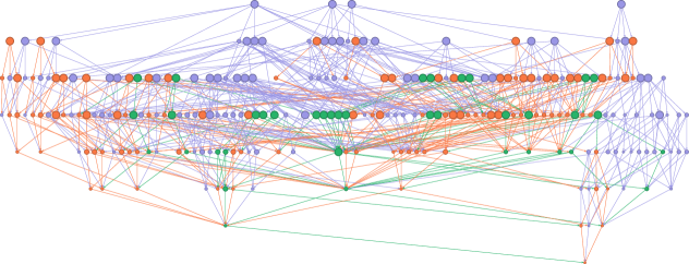
The resulting graph is given in Figure 1. The graph is topologically sorted, such that all the edges go from top to bottom. This presentation immediately draws attention to a number of facts. Firstly, we note that the graph contains a unique terminal vertex. This vertex corresponds to the rational points of with -invariant equal to , and its existence is a direct consequence Corollary 5.6. Secondly, the genus of the underlying curves does not monotonically decrease as the graph is traversed. This stems from the interplay between Theorem 2.15, which maps isolated points on higher genus curves to points on lower genus curves, and Theorem 2.16, which works in the other direction. However, the degree of the closed points does decrease monotonically from top to bottom, which is a consequence of the degree conditions in these two theorems.
Equipped with this quotient graph, we now aim to show that many of the vertices in this graph correspond to closed points which are not isolated. Consider a vertex of the quotient graph. This vertex corresponds to a set of closed points with the same isolated-ness, and, by the proof of Theorem 6.7, the closed point of corresponding to the double coset is a point in this set. The degree of this closed point can be computed using Theorem 4.18, while the number and genus of the connected components of can be computed using Remark 4.11. If the degree of the closed points is strictly greater than the product of the number and genus of the connected components of , then the closed point is not -isolated, by Theorem 2.17.
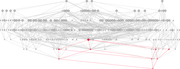
Iterating through all the vertices in the quotient graph and applying the above, we obtain Figure 2. The vertices for which Theorem 2.17 applies are in gray, while the subgraph induced by the remaining vertices is highlighted in red. We note that, out of the 252 vertices in the quotient graph, 243 can be shown to correspond to non-isolated closed points using the aforementioned theorem. The 9 remaining vertices correspond to modular curves and closed points precisely as described in Table 1, thus proving Theorem 6.4.
The remaining 9 vertices form a single connected subgraph of the quotient graph. Moreover, this subgraph contains a unique initial vertex. This vertex corresponds to the degree 18 points on the modular curve with -invariant . By the construction of the isolation graph, it thus suffices to show that any of these degree 18 points is isolated, as this will then imply that all the other vertices also correspond to isolated points. We record this in the following lemma, for future reference.
Lemma 6.8.
Suppose that one of the degree 18 closed points with -invariant on the modular curve is isolated. Then, all closed points described in Table 1 are isolated.
We tackle the problem of confirming that these degree 18 points are indeed isolated in the next section. In the meantime, we conclude this section with one final remark.
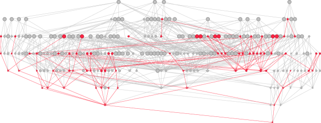
Remark 6.9.
Figure 3 again shows the quotient of the isolation graph discussed previously. The subgraph induced by the closed points lying on geometrically connected modular curves is highlighted in red. We note that this subgraph does not contain a unique terminal vertex; rather, there are three such vertices. In particular, for the two new terminal vertices, Corollary 5.6 cannot be proven if we restrict ourselves to maps between geometrically connected curves. This shows the importance of considering geometrically disconnected curves, even if one is solely interested in understanding isolated points on geometrically connected curves.
6.3 The closed points of Table 1 are isolated
In Section 6.1, we showed that the -invariant of a non-cuspidal, non-CM isolated closed point with rational -invariant on a modular curve of level 7 must equal . Moreover, in Section 6.2, we showed that the modular curve and the isolated closed point must be one of the pairs described in Table 1. Therefore, it remains to show that all the closed points of Table 1 are indeed isolated, to which this section is devoted to.
Theorem 6.10.
Let and be as described in Table 1. Then, is an isolated closed point of the modular curve .
Proof.
By Lemma 6.8, it suffices to prove that any of the degree 18 closed points with -invariant on the modular curve are isolated. Since , the Stein factorization of the modular curve is
By Theorem 2.7, it suffices to show that any of the degree 3 closed points on corresponding to the desired degree 18 closed points on are isolated. Let be the modular curve , where
Since , we obtain, by Theorem 4.15, a Cartesian square
where is the inclusion morphism . The morphism factors through the -map . Noting that , we can therefore rewrite the above commutative diagram as
where both squares are Cartesian. Since the composition is precisely the -map , it follows that the closed points of with -invariant are the closed points of lying above .
We know by [16, Equation 3-1] that a model for the modular curve over is given by the Klein quartic . Moreover, Halberstadt and Kraus give an explicit equation for the degree-168 -map ; see [16, Equation 3-10]. By base change to , this therefore gives an explicit model for , as well as the map . Using Magma, we can use this to explicitly compute the degree 3 points on lying above . Moreover, we can compute the dimension of the Riemann-Roch spaces of these points. In all cases, we find that the dimension of the Riemann-Roch space is always 1. Thus, all of the desired degree 3 points on are -isolated.
Finally, we compute the Mordell-Weil rank of the Jacobian of . We know, by [16, Section 8], that the Jacobian of is isogenous over to , where is the elliptic curve
Using Magma, we compute that the Mordell-Weil rank of is 0. Therefore, the Mordell-Weil rank of the Jacobian of is also 0. It follows that all closed points of are AV-isolated, thus completing the proof. ∎
7 Isolated points on the modular curves
In this section, we aim to use the results of Section 5 to give a conjectural classification of the non-cuspidal, non-CM isolated points with rational -invariant on the modular curves . This problem is closely related to the problem of determining the non-cuspidal, non-CM isolated points with rational -invariant on the modular curves , which has attracted much attention in recent literature. While the methods for tackling the first problem should be applicable to this second problem, the computations necessary for the first problem can already be found in the literature, while those for the second have not been carried out previously. Therefore, we limit ourselves to studying at present, and leave for future work.
The structure of the proof is similar to the one employed in the previous section. Firstly, we will use knowledge of the images of the Galois representations associated to elliptic curves defined over to restrict the -invariant of an isolated point on a modular curve . Secondly, we show that there are finitely many modular curves which must be checked for isolated points. Finally, we tackle each of these finite cases separately, finding all of the isolated points with rational -invariant on each modular curve.
The first part differs strongly from the classification of isolated points on modular curves of level 7. In the latter case, there are only finitely many possible images of the mod 7 Galois representation associated to an elliptic curve over , and the classification of such images can be found in the literature. However, in this case, if one were to apply Theorem 5.3, one would need a classification of all possible adelic Galois representations associated to elliptic curves over , which has not been completed. Moreover, even if such a classification were to exist, there are infinitely many exceptional adelic representations, leading one to have to consider infinitely many -invariants. Instead, we rely on the notion of agreeable closures, which was first defined in [25].
Definition 7.1.
Let be an open subgroup of , and let be the level of . Recall that . We define the agreeable closure of to be the subgroup
where denotes the subgroup of scalar matrices of . The agreeable closure is an open subgroup of whose level is only divisible by primes dividing .
Our aim is now to prove a generalization of Theorem 5.3 to agreeable closures. To do so, we first prove a stronger version of Corollary 5.8 in the case of .
Lemma 7.2.
Let , and be a non-cuspidal, non-CM isolated closed point with minimal representative . Let be the level of . Then the closed point corresponding to the -orbit of the geometric point is isolated.
Proof.
By definition, is the smallest integer such that contains the kernel of the map . Denote by the kernel of this map, and note that is a normal subgroup of . Therefore, by Theorem 5.7, the closed point corresponding to the geometric point is isolated. It remains to show that .
The subgroup contains the set
Since , it follows that . Let . Since , we have that . Moreover, by construction, is congruent to 1 modulo , and so is as well. Thus, . Since
we obtain that . Therefore, we have
Since has level , it contains the kernel . Hence, by Lemma 3.5, we obtain that
Thus, we have , and the result follows. ∎
Using this result, we may now prove the aforementioned generalization of Theorem 5.3.
Theorem 7.3.
Let , and be a non-cuspidal, non-CM isolated closed point with minimal representative . Let be the agreeable closure of . Then the closed point corresponding to the geometric point is isolated.
Proof.
Let be the level of , and the level of . In particular, note that divides . By Lemma 7.2, the closed point corresponding to the -orbit of the -point is isolated. The subgroup has level , and so contains both the product and the kernel . Moreover, contains the subgroup of scalar matrices, which we denote by abuse of notation. All three of these subgroups are normal subgroups of , and hence so is their product . This product is also an open subgroup of , since the kernel is open by definition. Note that we have
Therefore, since is isolated, so is , by Theorem 5.5. ∎
This result places much more stringent restrictions on the elliptic curve than results such as Theorem 5.3. Notably, assuming Serre’s uniformity conjecture, there are finitely many agreeable closures of , as ranges through all non-CM elliptic curves over . More importantly, a conjectural set of such agreeable closures has been computed by Zywina in [25]. We summarize these computations as follows.
Conjecture 7.4 ([25, Theorem 1.9, Section 14.3]).
Let be a non-CM elliptic curve over and a profinite level structure on . Let be the agreeable closure of the extended adelic Galois image . Then, one of the following hold:
-
•
is a geometrically connected curve of genus 0
-
•
is a geometrically connected curve of genus 1, and is infinite
-
•
is finite, and the group and the -invariant of are given in Table LABEL:tbl:isolated_points_x0:exceptional_j_invariants
| -invariant | Level of | Level of | ||
|---|---|---|---|---|
In tandem with Theorem 7.3, these computations strongly restrict the possible -invariants of non-cuspidal, non-CM isolated points with rational -invariant on the modular curves .
Theorem 7.5.
Assume that Conjecture 7.4 holds. Let , and be a non-cuspidal, non-CM isolated closed point with minimal representative , with . Then the -invariant is given in Table LABEL:tbl:isolated_points_x0:exceptional_j_invariants.
Proof.
Let be the agreeable closure of the extended adelic Galois image . By Theorem 7.3, the closed point corresponding to the -orbit of the -point is isolated. Note that the agreeable closure contains the extended adelic Galois image , and that . Therefore, by Theorem 4.24, the closed point has degree 1.
Since the point is isolated, by Theorem 2.17, the geometrically connected modular curve cannot have genus 0. Moreover, if the modular curve has genus 1, the image is a translate of , itself isomorphic to . Since is isolated, it follows that must have rank 0. Therefore, by Conjecture 7.4, the -invariant of is given in Table LABEL:tbl:isolated_points_x0:exceptional_j_invariants. ∎
We have now shown that the -invariant of every non-cuspidal, non-CM isolated closed point with rational -invariant on a modular curve must lie in the explicit finite set given in Table LABEL:tbl:isolated_points_x0:exceptional_j_invariants. Following the method outlined at the start of this section, we now show that most of the -invariants given in the aforementioned table do not give rise to such isolated points.
Theorem 7.6.
Proof.
By Theorem 7.5, the -invariant must be one of the 81 -invariants listed in Table LABEL:tbl:isolated_points_x0:exceptional_j_invariants. Therefore, suppose that the -invariant of is given in Table LABEL:tbl:isolated_points_x0:exceptional_j_invariants, but not given in Table 3. The image of the Galois representation of the elliptic curve is computed in [25], for some fixed profinite level structure . In particular, we can compute the level of the intersection , which is also recorded in Table LABEL:tbl:isolated_points_x0:exceptional_j_invariants.
By Lemma 7.2, since the point is isolated, so is the point corresponding to the -orbit of the geometric point . Therefore, it suffices to show that the modular curves do not contain an isolated closed point with -invariant equal to , for all divisors of .
For each such divisor , the closed points of with -invariant equal to are in bijection with the double cosets , by Theorem 4.18. As the extended adelic Galois image of is known, we may compute the degree of each of these closed points using the aforementioned theorem. For each such closed point, this degree exceeds the genus of the modular curve , and so the closed point cannot be isolated, by Theorem 2.17.
These computations are implemented in the file isolated_points_x0.m. As an example, let be the elliptic curve 61347.bb1 with -invariant . The extended adelic Galois image has level 78, and is given by the preimage of the subgroup
The intersection has level 26, and so it suffices to show that there are no isolated points with the given -invariant on the modular curves , where . The modular curves , and all have genus 0, and so there are no isolated points on these modular curves by Theorem 2.17. The modular curve however, has genus 2.
The extended mod-26 Galois image of is given by the reduction modulo 26 of . For each conjugate of , we compute the index , and find that it is either 18 or 24. Therefore, by Theorem 4.18, the closed points of with -invariant must have degree 18 or 24. In both cases, this degree exceeds the genus of , and so, by Theorem 2.17, these closed points cannot be isolated. ∎
| Minimal | |||
|---|---|---|---|
| 1 | 1 | ||
| 1 | |||
| 1 | 1 | ||
| 1 | |||
| 1 | |||
| 1 | |||
| 1 | 1 | ||
| 1 | |||
| 1 | 1 | ||
| 1 | |||
| 1 | |||
| 1 | |||
| 2 | 1 | ||
| 1 |
It remains to verify the rest of Table 3, namely that for each -invariant listed in the table, there exists an isolated closed point on the corresponding modular curve .
Theorem 7.7.
Let and be as given in Table 3. Then, there exists an isolated closed point with -invariant equal to . Moreover, is the smallest integer such that contains an isolated closed point with the given -invariant.
Proof.
Fix a -invariant from Table 3, and let be the smallest integer such that contains an isolated closed point with the given -invariant. By Lemma 7.2, must divide the level of , for any elliptic curve with the given -invariant. Note that this level is given in Table LABEL:tbl:isolated_points_x0:exceptional_j_invariants.
The integer given in Table 3 is the smallest integer dividing the level of such that the modular curve has genus greater than 0. Therefore, the second part of the result follows from the first part, by Theorem 2.17.
Consider now the modular curve given in Table 3. The extended adelic Galois image is known by [25], for some elliptic curve with the given -invariant and some profinite level structure on . Using this, we compute that the extended mod- Galois image of is conjugate to a subgroup of . Therefore, by Theorem 4.18, there exists a rational point with the given -invariant.
If has genus 1, the explicit models of in the LMFDB [20] show that has rank 0, and so the set is finite. If however, then has genus 2, and so, by Faltings’s theorem, the set is also finite. Therefore, by Theorem 2.3, any rational point on is isolated. Therefore, there exists an isolated closed point with the given -invariant. ∎
Remark 7.8.
Table 3 solely lists the minimal integer such that the modular curve contains an isolated closed point with the given -invariant. The existence of other isolated closed points with the same -invariant on the modular curves , where is a multiple of , is still an open problem. In fact, it is still unknown whether the set of modular curves containing such an isolated point is finite or infinite.
Appendix A Divisor and Picard schemes of geometrically reducible varieties
The study of the divisor and Picard schemes of a geometrically integral variety is well-established, however much less is known in the context of geometrically reducible varieties. In this appendix, we show how the Stein factorization of a geometrically reducible variety can be used to give a link between these two settings. In particular, we show that the divisor and Picard schemes of a geometrically reducible variety are given by Weil restrictions, and deduce some consequences on the structure of the Abel map between the two schemes.
We use the notation of Section 2 throughout. Namely, let be a smooth, projective integral scheme over a number field . We denote by the divisor scheme of , by the Picard scheme of , and by the Abel map between the two. Let
be the Stein factorization of the structure morphism , where is a finite extension of number fields. In particular, is étale and is smooth, projective and geometrically integral. We use analogous notation to denote the divisor and Picard schemes of .
Throughout this appendix, and the body of the main paper, we will often rely on the properties of Weil restrictions under étale morphisms. While many such properties have already been made explicit in the literature, we have been unable to find a reference for the following statement on surjectivity.
Theorem A.1.
Let be a finite étale morphism of schemes. Let be a surjective morphism of -schemes, and assume that the Weil restrictions and exist as schemes. Then is surjective. In particular, if the structure morphism is surjective, then so is the morphism .
Proof.
Let , and . To show that is surjective, it suffices to check this over each geometric fiber of . As Weil restriction commutes with base change, we may therefore assume that for an algebraically closed field .
Since is finite étale, is isomorphic to , for some natural number . By definition, the map equals the map . Since is surjective and is algebraically closed, the latter map is also surjective. Therefore, is surjective.
The last statement follows from the fact that the morphism is the Weil restriction of the structure morphism , and the above. ∎
Firstly, we show that the Picard scheme is isomorphic to the Weil restriction of the Picard scheme . This fact is stated, without proof, in much greater generality by Grothendieck in [15, Proposition 6.1]. However, we are only able to provide a proof when the extension is separable. The separable case is also treated in [19, Lemma 3.7]. We give a different proof, as the specifics of the isomorphism will be used later.
Theorem A.2.
Let and be as above. Then there exists an isomorphism of group schemes
Proof.
Since exists as a scheme, it suffices to establish an isomorphism for all -schemes , which is functorial in .
Let be a -scheme. Define an fppf-cover of to be the morphism
where is a covering in the fppf topology. As is discussed in [18, p.17], the set consists of invertible sheaves , where is an fppf-cover of , and such that there exists an fppf-cover such that the pullbacks of with respect to , for both projections , are isomorphic. Moreover, two such sheaves and define the same point of if and only if there exists an fppf-cover such that the pullbacks of and to are isomorphic. A similar description holds for .
Consider a point represented by an invertible sheaf . Since , we can consider as an element of . Since is an fppf-cover, so is the base change . It is straightforward to check that represents a point of , and that the latter does not depend on the choice of representative of . This defines the group homomorphism .
Let be a morphism of -schemes, and let be a point represented by an invertible sheaf . The morphism maps the point to the point represented by the pullback of with respect to the morphism . This latter morphism is the same as the morphism , since both correspond to the base change of the morphism with respect to . This establishes the functoriality of in .
Consider now a point of represented by an invertible sheaf . Let be the Galois closure of the field extension . Since is a separable extension, we have , where . Therefore, we obtain that . Let be the fiber product , and denote by its fiber over the -th point , so that . Note that, since the morphism is an fppf-cover, so too is .
Consider the product , which, by the above, is an fppf-cover of . Since the morphism is an fppf-cover, it follows that is also an fppf-cover of . By construction, we have
The projection morphism factors through , with the morphism given by the projection map over the -th point . Note that this morphism is an fppf-cover. Consider the invertible sheaf given by the pullback of with respect to the composition . By applying the above construction repeatedly, one can show that defines a point of , and that this point does not depend on the choice of and . Therefore, we obtain a map .
The above construction can also be summarized with the following commutative diagram, in which all squares are Cartesian. We use fppf to indicate fppf-covers.
It remains to show that and are inverses. Throughout, we use the following fact, which follows from the explicit description of given above: let be a representative for a point , and let be an fppf-cover of . Then the pullback of with respect to is also a representative of .
Let be a point represented by an invertible sheaf . Using the notation in the diagram above, the point is represented by the pullback of with respect to the map . By the above fact, this is precisely , and so the composition is the identity.
On the other hand, let be a point represented by an invertible sheaf . Again, we employ the notation in the diagram above, where is replaced by . Then, the point is represented by the pullback of with respect to the map . By construction, we have
Therefore, for all , and so the morphism is equal to the pullback of the morphism with respect to the morphism , up to an isomorphism of . Therefore, the point is represented by the pullback of with respect to the map . By the above fact, it follows that , and so the composition is the identity.
Thus, is an isomorphism for all -schemes , completing the proof. ∎
Similarly, the divisor scheme is isomorphic to the Weil restriction of the divisor scheme . Moreover, this isomorphism is compatible with the isomorphism of Picard schemes just described, as the following theorem shows.
Theorem A.3.
Let and be as above. Then there exists an isomorphism of schemes
Moreover, there is a commutative diagram
Proof.
To prove the first part of the theorem, it suffices to give an isomorphism for all -schemes , which is functorial in .
Let be a -scheme. By definition, is the set of relative effective Cartier divisors on , that is to say, the set of effective Cartier divisors on which are flat over . Similarly, is the set of effective Cartier divisors on which are flat over .
Let be a relative effective Cartier divisor on . As the schemes and are equal, is also an effective Cartier divisor on . By definition, the composition is flat. Moreover, since is a finite separable field extension, the morphism is unramified. Therefore, the composition is also flat. In other words, is flat over , and so is a relative effective Cartier divisor on . This defines the map .
Let be a morphism of -schemes. The map is given by the pullback with respect to the morphism . Similarly, the map is given by the pullback with respect to the morphism . Since these two morphisms are equal, and pullback of relative effective Cartier divisors does not depend on the base, the functoriality of the map follows.
By construction, the map is injective. Moreover, since is a field extension, the morphism is flat. Therefore, any relative effective Cartier divisor on is also flat over . Thus, the map is also surjective, and hence is an isomorphism.
To show the second part of the theorem, it suffices to show that the following diagram commutes for all -schemes T.
Let be a -scheme, and be a relative effective Cartier divisor on . By definition, the point is represented by the invertible sheaf . It follows that the point is represented by the invertible sheaf . On the other hand, since maps to itself, the point is represented by the invertible sheaf . As the schemes and coincide, the result follows. ∎
This identification between the divisor and Picard schemes of a geometrically reducible variety and the Weil restriction of the corresponding schemes of the Stein factorization allows us to carry some of the results for the geometrically integral case to the geometrically reducible case. For instance, the Abel map is proper in both settings, as the following theorem shows.
Theorem A.4.
Let and be as above. Then the Abel map is proper.
Proof.
By Theorem A.3, it suffices to show that the Weil restriction is proper. As the structure map is smooth and projective, with geometrically integral fibers, the Abel map is proper by [18, Exercise 4.12]. Moreover, the morphism is finite and étale, and so the Weil restriction is proper by [17, Proposition 6.2.9]. ∎
In much the same way, the description of the Abel map in terms of Weil restrictions leads to a concrete description of the fibers of the Abel map in the case of geometrically reducible varieties.
Theorem A.5.
Let and be as above. Let be an invertible sheaf on , and the corresponding point of the Picard scheme. Then, the fiber is isomorphic to , where .
Proof.
By Theorem A.3, we have a commutative diagram
As both and are isomorphisms, the fiber is isomorphic to the fiber . By [7, Proposition A.5.2 (3)] and [7, Proposition A.5.7], the fiber is isomorphic to the Weil restriction , where is the point corresponding to under the isomorphism . In particular, using the explicit description of , we have . Therefore, we have
By [2, Proposition 8.2.7], since is geometrically integral, the fiber is represented by , for some -module . Moreover, every -module is cohomologically flat over in dimension zero, as is a field. Therefore, the aforementioned result also shows that is locally free, and is isomorphic to the dual of , where is the structure map. Thus, we obtain that , where is the dimension of the -vector space . By [21, Corollary II.5.2], it follows that , as required. ∎
Finally, one can give a description of the image as a subset of . While not as explicit as in the case of geometrically integral varieties, this is description still proves to be very useful in Section 2.
Theorem A.6.
Let and be as above. Then there exists a subgroup such that
Moreover, the quotient group is torsion.
Proof.
By Theorem A.3, we have the following commutative diagram
where both and are isomorphisms. Therefore, we have
Since is geometrically integral, by [2, Proposition 8.1.4], we obtain the following exact sequence
In particular, the group of -points of the relative Picard functor embeds into the group of -points of the Picard scheme . Moreover, the quotient group is a subgroup of the Brauer group of , and hence is a torsion group.
Since the Abel map factors through the relative Picard functor , we have
Let , and consider the fiber . Since , represents the class of an invertible sheaf on . By Theorem A.5, the fiber is isomorphic to , for some . Moreover, since , the fiber is not empty, and so . In particular, the set is non-empty, and so . Therefore, we have shown that
Using , since is an isomorphism, we have
Moreover, denoting by the subgroup of , the quotient group is torsion.
References
- [1] M. Artin, J.. Bertin, M. Demazure, P. Gabriel, A. Grothendieck, M. Raynaud and J.-P. Serre “Schémas en groupes. Fasc. 2a: Exposés 5 et 6” Deuxième édition, Séminaire de Géométrie Algébrique de l’Institut des Hautes Études Scientifiques, 1963/64, dirigé par Michel Demazure et Alexander Grothendieck Institut des Hautes Études Scientifiques, Paris, 1963, pp. ii+180 pp. (not consecutively paged)
- [2] Siegfried Bosch, Werner Lütkebohmert and Michel Raynaud “Néron models” 21, Ergebnisse der Mathematik und ihrer Grenzgebiete (3) [Results in Mathematics and Related Areas (3)] Springer-Verlag, Berlin, 1990, pp. x+325 DOI: 10.1007/978-3-642-51438-8
- [3] Wieb Bosma, John Cannon and Catherine Playoust “The Magma algebra system. I. The user language” Computational algebra and number theory (London, 1993) In J. Symbolic Comput. 24.3-4, 1997, pp. 235–265 DOI: 10.1006/jsco.1996.0125
- [4] Abbey Bourdon, Özlem Ejder, Yuan Liu, Frances Odumodu and Bianca Viray “On the level of modular curves that give rise to isolated -invariants” In Adv. Math. 357, 2019, pp. 106824\bibrangessep33 DOI: 10.1016/j.aim.2019.106824
- [5] Abbey Bourdon, David R. Gill, Jeremy Rouse and Lori D. Watson “Odd degree isolated points on with rational -invariant” In Res. Number Theory 10.1, 2024, pp. Paper No. 5\bibrangessep32 DOI: 10.1007/s40993-023-00488-0
- [6] Abbey Bourdon, Sachi Hashimoto, Timo Keller, Zev Klagsbrun, David Lowry-Duda, Travis Morrison, Filip Najman and Himanshu Shukla “Towards a classification of isolated -invariants”, 2024 arXiv: https://arxiv.org/abs/2311.07740
- [7] Brian Conrad, Ofer Gabber and Gopal Prasad “Pseudo-reductive groups” 26, New Mathematical Monographs Cambridge University Press, Cambridge, 2015, pp. xxiv+665 DOI: 10.1017/CBO9781316092439
- [8] P. Deligne and M. Rapoport “Les schémas de modules de courbes elliptiques” In Modular functions of one variable, II (Proc. Internat. Summer School, Univ. Antwerp, Antwerp, 1972) Vol. 349, Lecture Notes in Math. Springer, Berlin-New York, 1973, pp. 143–316
- [9] Fred Diamond and Jerry Shurman “A first course in modular forms” 228, Graduate Texts in Mathematics Springer-Verlag, New York, 2005, pp. xvi+436
- [10] Özlem Ejder “Isolated points on with rational -invariant” In Res. Number Theory 8.1, 2022, pp. Paper No. 16\bibrangessep7 DOI: 10.1007/s40993-022-00313-0
- [11] Gerd Faltings “The general case of S. Lang’s conjecture” In Barsotti Symposium in Algebraic Geometry (Abano Terme, 1991) 15, Perspect. Math. Academic Press, San Diego, CA, 1994, pp. 175–182
- [12] Gerhard Frey “Curves with infinitely many points of fixed degree” In Israel J. Math. 85.1-3, 1994, pp. 79–83 DOI: 10.1007/BF02758637
- [13] A. Grothendieck “Éléments de géométrie algébrique. I. Le langage des schémas.” In Inst. Hautes Études Sci. Publ. Math., 1960, pp. 228 URL: http://www.numdam.org/item?id=PMIHES_1960__4__228_0
- [14] A. Grothendieck “Éléments de géométrie algébrique. IV. Étude locale des schémas et des morphismes de schémas IV” In Inst. Hautes Études Sci. Publ. Math., 1967, pp. 361 URL: http://www.numdam.org/item?id=PMIHES_1967__32__361_0
- [15] Alexander Grothendieck “Technique de descente et théorèmes d’existence en géométrie algébrique. V. Les schémas de Picard: théorèmes d’existence” In Séminaire Bourbaki, Vol. 7 Soc. Math. France, Paris, 1995, pp. Exp. No. 232\bibrangessep143–161
- [16] Emmanuel Halberstadt and Alain Kraus “Sur la courbe modulaire ” In Experiment. Math. 12.1, 2003, pp. 27–40 URL: http://0-projecteuclid-org.pugwash.lib.warwick.ac.uk/euclid.em/1064858782
- [17] Lena Ji, Shizhang Li, Patrick McFaddin, Drew Moore and Matthew Stevenson “Weil restriction for schemes and beyond” In Stacks Project Expository Collection (SPEC) 480, London Math. Soc. Lecture Note Ser. Cambridge Univ. Press, Cambridge, 2022, pp. 194–221
- [18] Steven L. Kleiman “The Picard scheme”, 2005 arXiv:math/0504020 [math.AG]
- [19] Alexandros Konstantinou and Adam Morgan “On Galois covers of curves and arithmetic of Jacobians”, 2024 arXiv: https://arxiv.org/abs/2407.18258
- [20] The LMFDB Collaboration “The L-functions and modular forms database” [Online; accessed 20 November 2024], https://beta.lmfdb.org, 2024
- [21] David Mumford “Abelian varieties” 5, Tata Institute of Fundamental Research Studies in Mathematics Tata Institute of Fundamental Research, Bombay; by Oxford University Press, London, 1970, pp. viii+242
- [22] Jeremy Rouse, Andrew V. Sutherland and David Zureick-Brown “-adic images of Galois for elliptic curves over (and an appendix with John Voight)” With an appendix with John Voight In Forum Math. Sigma 10, 2022, pp. Paper No. e62\bibrangessep63 DOI: 10.1017/fms.2022.38
- [23] Andrew V. Sutherland “A local-global principle for rational isogenies of prime degree” In J. Théor. Nombres Bordeaux 24.2, 2012, pp. 475–485 URL: http://0-jtnb-cedram-org.pugwash.lib.warwick.ac.uk/item?id=JTNB_2012__24_2_475_0
- [24] Bianca Viray and Isabel Vogt “Isolated and parameterized points on curves”, 2024 arXiv: https://arxiv.org/abs/2406.14353
- [25] David Zywina “Explicit open images for elliptic curves over ”, 2024 arXiv: https://arxiv.org/abs/2206.14959
- [26] David Zywina “On the possible images of the mod representations associated to elliptic curves over ”, 2015 arXiv: https://arxiv.org/abs/1508.07660