Pontryagin-Guided Direct Policy Optimization Framework for Merton’s Portfolio Problem

Abstract

We present a Pontryagin-Guided Direct Policy Optimization (PG-DPO) framework for Merton’s portfolio problem, unifying modern neural-network-based policy parameterization with the costate (adjoint) viewpoint from Pontryagin’s Maximum Principle (PMP). Instead of approximating the value function (as in “Deep BSDE”), we track a policy-fixed backward SDE for the adjoint variables, allowing each gradient update to align with continuous-time PMP conditions. This setup yields locally optimal consumption and investment policies that are closely tied to classical stochastic control. We further incorporate an alignment penalty that nudges the learned policy toward Pontryagin-derived solutions, enhancing both convergence speed and training stability. Numerical experiments confirm that PG-DPO effectively accommodates both consumption and investment, achieving strong performance and interpretability without requiring large offline datasets or model-free reinforcement learning.

1 Introduction

Merton’s portfolio optimization problem (Merton,, 1971) is a cornerstone of mathematical finance, aiming to specify optimal investment and consumption decisions in a continuous-time market. Classical treatments (e.g., Karatzas & Shreve,, 1998; Yong & Zhou,, 1999; Pham,, 2009) exploit the problem’s analytical tractability to derive closed-form solutions under specific assumptions, such as constant coefficients or complete markets. In real-world settings, however, these idealized conditions are often not met, prompting practitioners to rely on data-driven methods that do not assume closed-form solutions. By parameterizing the policy $\bigl{(}\pi_{\theta},C_{\phi}\bigr{)}$ with neural networks and defining a suitable objective $J(\theta,\phi)$, one can use gradient-based learning (e.g., stochastic gradient descent) to iteratively improve the policy. Such deep-learning-based approaches have shown promise for high-dimensional state spaces, path dependence, and market frictions (Han & E,, 2016; Han et al.,, 2018; Beck et al.,, 2019; Buehler et al.,, 2019; Becker et al.,, 2019; Zhang & Zhou,, 2019; Reppen et al.,, 2023; Reppen & Soner,, 2023).

Despite these advances, a purely empirical or “black-box” gradient approach may overlook the continuous-time optimal control perspective. Without classical stochastic control principles as guidance, there is no clear guarantee that iterative updates will converge to a Pontryagin-aligned policy—that is, one satisfying the adjoint-based optimality conditions in continuous time. Recent studies (e.g., Reppen et al.,, 2023; Reppen & Soner,, 2023) highlight this tension: while purely data-driven methods can achieve high performance in practice, they may not incorporate the deeper theoretical underpinnings of optimal control. Other works, such as Dai et al., (2023), adopt model-free reinforcement learning, which requires extensive exploration and often omits consumption to focus on investment alone.

A different perspective is offered by the so-called “Deep BSDE” methodology, pioneered by Weinan E and collaborators (e.g., Han et al.,, 2018; Weinan,, 2017), which focuses on approximating the value function (i.e., solving the Hamilton–Jacobi–Bellman equation) via a forward–backward SDE, then infers the policy once the value function is estimated. By contrast, our approach is fundamentally adjoint-based: rather than approximating the value function, we track costate (adjoint) variables through a policy-fixed backward SDE and use them to guide parameter updates directly. In addition, we implement this scheme via backpropagation-through-time (BPTT), unrolling the system dynamics in discrete steps and enabling single-path simulation for each node. While both Deep BSDE and our Pontryagin-guided approach employ neural networks and SDEs, the difference in what is learned (value function vs. adjoint) and how it is integrated (decoupled vs. direct BPTT) can yield distinct interpretability and computational trade-offs.

Our framework adopts what we call a Pontryagin-Guided Direct Policy Optimization (PG-DPO) viewpoint. We treat the Merton problem as a continuous-time stochastic control system but solve it through direct neural-network-based optimization. Specifically, we embed Pontryagin’s Maximum Principle (PMP) (Pontryagin,, 2018) into a discrete-time training loop, interpreting each gradient step as an approximation to the continuous-time adjoint. This preserves the convenience of automatic differentiation and mini-batch simulation while offering a principled control-theoretic justification of policy improvement. We also incorporate both consumption and investment into the policy, a combination seldom tackled simultaneously by purely data-driven methods yet crucial in real-world portfolio planning.

Our numerical experiments and theoretical analyses demonstrate that this direct policy optimization (DPO) (Reppen et al.,, 2023; Reppen & Soner,, 2023) approach converges to stationary policies that are strongly aligned with Pontryagin’s conditions. Moreover, viewing the adjoint through the Pontryagin lens facilitates an alignment penalty (or regularization) that can speed up convergence. This additional penalty encourages the network’s consumption and investment policies to stay near Pontryagin-derived controls at each time instant, thereby improving training efficiency and stability in practice. In many cases, the policy converges to a local optimum that remains consistently Pontryagin-aligned and does so without relying on large offline datasets or purely model-free RL techniques.

Several aspects of this paper can be summarized as follows. First, we propose a Pontryagin-Guided DPO scheme that incorporates Pontryagin’s Maximum Principle in a discrete-time neural network framework. Each gradient update is interpreted in terms of the adjoint (costate) perspective, providing a more transparent route to near-optimal solutions than opaque gradient-based updates alone. Second, we add an adjoint-based alignment penalty, encouraging the neural policy to stay close to locally Pontryagin-optimal controls and thereby taking advantage of suboptimal adjoint estimates for faster convergence. Although we only guarantee local optimality, this “soft constraint” often yields notable improvements in training efficiency and stability. Third, by directly tackling both consumption and investment in the Merton problem, we address a more challenging scenario than usual in data-driven approaches. Our method converges reliably, uses rolling simulations (thus mitigating overfitting), and handles the entire state-time domain with a single neural network. Finally, the Pontryagin viewpoint supports interpretability—adjoint variables $\lambda_{t}$ and $Z_{t}$ are made explicit—while preserving the flexibility of modern deep-learning tools. This synergy can naturally extend to more general setups involving jumps, constraints, or multi-asset portfolios.

Section 2 reviews the continuous-time Merton formulation, emphasizing the interplay of consumption and investment. Section 3 revisits Pontryagin’s Maximum Principle and re-expresses Merton’s SDE via a forward–backward viewpoint, setting the stage for our adjoint-based approach. In Section 4, we contrast our method with “Deep BSDE” frameworks that approximate the value function instead of the adjoint. Next, Section 5 explains the discrete-time updates that approximate the continuous-time Pontryagin flow, including a normalization penalty for faster convergence. In Section 6, we use a stochastic approximation viewpoint (Robbins–Monro theory) to show that our method converges locally. Section 7 presents numerical experiments demonstrating convergence to robust local optima aligned with Pontryagin’s conditions. Finally, Section 8 offers concluding remarks and discusses possible extensions that further bridge deep learning and stochastic control.

2 Continuous-Time Formulation of the Merton Portfolio Problem

We consider the Merton portfolio optimization problem, where an investor allocates wealth between a risky asset $S_{t}$ and a risk-free asset $B_{t}$. The risky asset follows a geometric Brownian motion:

$$dS_{t}=\mu S_{t}\,dt+\sigma S_{t}\,dW_{t},$$

and the risk-free asset evolves as

$$dB_{t}=rB_{t}\,dt.$$

The investor’s wealth $X_{t}$ evolves under continuous consumption $C_{t}$ and a proportion $\pi_{t}$ invested in the risky asset:

$$dX_{t}=(rX_{t}+\pi_{t}(\mu-r)X_{t}-C_{t})\,dt+\pi_{t}\sigma X_{t}\,dW_{t},\quad X_{0}=x_{0}>0.$$

We consider the objective:

$$J(\theta,\phi)=\mathbb{E}\left[\int_{0}^{T}e^{-\rho t}U(C_{t})\,dt+\kappa e^{-\rho T}U(X_{T})\right],$$

where $U(x)=\frac{x^{1-\gamma}}{1-\gamma}$ is a CRRA utility function, $\rho>0$ is a discount factor, and $\kappa>0$ is a parameter controlling the relative importance of terminal wealth (bequest). We parametrize the policies using neural networks:

$$\pi_{t}=\pi_{\theta}(t,X_{t}),\quad C_{t}=C_{\phi}(t,X_{t}).$$

These neural-network-based controls must be admissible, ensuring well-posedness of the state dynamics, integrability of payoffs, and non-explosion of the wealth process. 1. They must be adapted and measurable, meaning that $(\pi_{t},C_{t})$ are progressively measurable with respect to the filtration generated by $(W_{t})$ and therefore depend only on current information. 2. Boundedness or growth conditions must be satisfied: there must exist constants ensuring $|\pi_{t}|\leq M_{\pi}$ for some $M_{\pi}>0$ and $C_{t}\geq 0$ does not grow too quickly. 3. To ensure $J(\theta,\phi)$ is finite, integrability requirements must hold, i.e., $\mathbb{E}\bigl{[}\int_{0}^{T}e^{-\rho t}U(C_{t})\,dt+\kappa e^{-\rho T}U(X_{T})\bigr{]}<\infty.$ 4. Finally, consumption must be nonnegative $(C_{t}\geq 0)$, and $\pi_{t}$ must maintain $X_{t}$ as a nonnegative (or positive) quantity almost surely. In practice, neural-network-based controls can be designed (e.g., through appropriate activation functions) to enforce such feasibility constraints automatically.

Under these conditions, the state SDE is well-defined, $X_{t}$ remains in a suitable domain, and $J(\theta,\phi)$ is finite. A key property of the Merton problem is the strict concavity of $U(x)$, ensuring uniqueness of the global maximum. Classical results (Merton, (1971), Karatzas & Shreve, (1998), Yong & Zhou, (1999)) show that any stationary point of $J(\theta,\phi)$ is in fact the unique global maximizer. This uniqueness is fundamental to the theoretical analysis we develop.

In the classical Merton problem with CRRA utility and no bequest ($\kappa=0$), closed-form solutions are well-known. For example, consider the infinite-horizon setting with a discount rate $\rho>0$. The optimal investment and consumption rules are constants:

$$\pi_{t}^{*}=\frac{\mu-r}{\gamma\sigma^{2}},\quad C_{t}^{*}=\nu X_{t},\quad\text{where }\nu=\left(\rho-(1-\gamma)\left(\frac{(\mu-r)^{2}}{2\sigma^{2}\gamma}+r\right)\right)/\gamma.$$

This form shows that a constant fraction of wealth $\pi_{t}^{*}$ is invested in the risky asset, and consumption is proportional to current wealth with rate $\nu$.

For the finite-horizon problem or when a bequest term ($\kappa>0$) is included, the closed-form solutions become slightly more involved but remain known in closed form. As an example, with finite horizon $T$ and $\kappa>0$, the optimal consumption can be expressed as:

$$c(W,t)=\nu\left(1+(\nu\epsilon-1)e^{-\nu(T-t)}\right)^{-1}W,\quad\text{where }\epsilon=\kappa^{1/\gamma}$$

with the same $\nu$ defined above. As $T\to\infty$, this converges to the infinite-horizon solution. These closed-form formulas serve as benchmarks, confirming that the policy learned by our neural network approach indeed converges to the theoretically optimal strategy.

3 Pontryagin’s Maximum Principle and Its Application to Merton’s Problem

3.1 Pontryagin’s Maximum Principle

Pontryagin’s Maximum Principle (PMP) provides necessary conditions for optimality in a broad class of continuous-time optimal control problems (see, e.g., (Pontryagin,, 2018; Pardoux & Peng, 1990a, ; Fleming & Soner,, 2006; Yong & Zhou,, 1999; Pham,, 2009)). By framing the Merton problem as a stochastic optimal control problem, we can apply PMP to derive adjoint equations and optimality conditions. These conditions lead to a representation of the problem as a coupled forward-backward system, where the backward stochastic differential equation (BSDE) for the adjoint variables $(\lambda_{t}^{*},Z_{t}^{*})$ encapsulates the sensitivity of the optimal value function $J^{*}$ (Pardoux & Peng, 1990a, ; Yong & Zhou,, 1999).

Consider a stochastic control problem with state dynamics:

$$dX_{t}=b(t,X_{t},u_{t})\,dt+\sigma(t,X_{t},u_{t})\,dW_{t},\quad X_{0}=x_{0},$$

and an objective functional:

$$J(u)=\mathbb{E}\left[\int_{0}^{T}g(t,X_{t},u_{t})\,dt+G(X_{T})\right].$$

If $u_{t}^{*}$ is the optimal control that achieves the supremum of $J(u)$, let $J^{*}$ be the corresponding optimal value function. Pontryagin’s Maximum Principle (PMP) provides a set of necessary conditions for optimality (Pontryagin,, 2018; Fleming & Soner,, 2006; Yong & Zhou,, 1999). It does so by introducing the Hamiltonian $\mathcal{H}$ and adjoint variables $(\lambda_{t}^{*},Z_{t}^{*})$. Specifically, we define the Hamiltonian as:

$$\mathcal{H}(t,X_{t},u_{t},\lambda_{t},Z_{t})=g(t,X_{t},u_{t})+\lambda_{t}b(t,X_{t},u_{t})+Z_{t}\sigma(t,X_{t},u_{t}).$$

Under the optimal control $u_{t}^{*}$, the adjoint process $\lambda_{t}^{*}$ can be interpreted as $\lambda_{t}^{*}=\frac{\partial J^{*}}{\partial X_{t}}$, the sensitivity of the optimal value $J^{*}$ with respect to the state $X_{t}$. The pair $(\lambda_{t}^{*},Z_{t}^{*})$ satisfies the backward stochastic differential equation (BSDE):

$$d\lambda_{t}^{*}=-\frac{\partial\mathcal{H}}{\partial X}(t,X_{t}^{*},u_{t}^{*},\lambda_{t}^{*},Z_{t}^{*})\,dt+Z_{t}^{*}\,dW_{t},\quad\lambda_{T}^{*}=\frac{\partial G}{\partial X}(X_{T}^{*}).$$

Solving this BSDE together with the forward SDE for $X_{t}^{*}$ forms a coupled forward-backward SDE system. From this system, one obtains not only the optimal state trajectory $X_{t}^{*}$ and the adjoint processes $(\lambda_{t}^{*},Z_{t}^{*})$, but also characterizes the optimal control $u_{t}^{*}$ by maximizing the Hamiltonian with respect to $u$ at each time $t$.

By selecting $u_{t}^{*}$ to maximize $\mathcal{H}$ at each time instant, Pontryagin’s Maximum Principle transforms the original problem into a condition that locally characterizes optimal controls. The resulting forward-backward SDE system provides a principled way to compute or approximate $u_{t}^{*}$, connecting value sensitivities ($\lambda_{t}^{*}$), noise sensitivities ($Z_{t}^{*}$), and the evolving state $X_{t}^{*}$ in a unified mathematical framework (Fleming & Soner,, 2006; Yong & Zhou,, 1999; Pham,, 2009).

3.2 Pontryagin Adjoint Variables and Parameter Gradients in the Merton Problem

In this subsection, we combine two key components for handling both the optimal Merton problem and suboptimal parameterized policies. First, we restate the Pontryagin conditions for the Merton setup, which yield the optimal relationships among $(\lambda_{t}^{*},Z_{t}^{*},\pi_{t}^{*},C_{t}^{*})$. Second, we explain how to generalize these adjoint variables to a policy-fixed BSDE in the suboptimal setting and derive corresponding parameter gradients.

3.2.1 Pontryagin Formulation for Merton’s Problem

Recall that the Merton problem aims to maximize

$$J(\theta,\phi)\;=\;\mathbb{E}\Bigl{[}\int_{0}^{T}e^{-\rho t}U(C_{t})\,dt\;+\;\kappa e^{-\rho T}U(X_{T})\Bigr{]},$$

subject to

$$dX_{t}\;=\;(rX_{t}+\pi_{t}(\mu-r)X_{t}-C_{t})\,dt\;+\;\pi_{t}\sigma X_{t}\,dW_{t},$$

where $U(\cdot)$ is a CRRA utility function, $\rho>0$ is a discount rate, and $\kappa>0$ represents the bequest weight. Define the Hamiltonian:

$$\mathcal{H}(t,X_{t},\pi_{t},C_{t},\lambda_{t},Z_{t})\;=\;e^{-\rho t}U(C_{t})\;+\;\lambda_{t}\bigl{[}rX_{t}+(\mu-r)\pi_{t}X_{t}-C_{t}\bigr{]}\;+\;Z_{t}\,\pi_{t}\sigma X_{t}.$$

From Pontryagin’s Maximum Principle (PMP), the optimal controls $(\pi_{t}^{*},C_{t}^{*})$ maximize $\mathcal{H}$ pointwise in $(\pi_{t},C_{t})$. Differentiating w.r.t. $C_{t}$ and $\pi_{t}$ and setting to zero:

1. Consumption:

   $$\frac{\partial\mathcal{H}}{\partial C_{t}}\;=\;e^{-\rho t}U^{\prime}(C_{t}^{*})\;-\;\lambda_{t}\;=\;0\quad\Longrightarrow\quad U^{\prime}(C_{t}^{*})\;=\;e^{\rho t}\lambda_{t}^{*}.$$

   Since $U^{\prime}(x)=x^{-\gamma}$, it follows that

   $$C_{t}^{*}\;=\;\Bigl{(}e^{\rho t}\,\lambda_{t}^{*}\Bigr{)}^{-\frac{1}{\gamma}}.$$

2. Investment:

   $$\frac{\partial\mathcal{H}}{\partial\pi_{t}}\;=\;(\mu-r)\lambda_{t}X_{t}+Z_{t}\sigma X_{t}\;=\;0\quad\Longrightarrow\quad(\mu-r)\lambda_{t}^{*}+Z_{t}^{*}\sigma\;=\;0.$$

   Thus, the optimal adjoint processes satisfy $Z_{t}^{*}=-\frac{(\mu-r)}{\sigma}\,\lambda_{t}^{*}$.

Hence, under PMP, the pair $(\lambda_{t}^{*},Z_{t}^{*})$ links directly to $(\pi_{t}^{*},C_{t}^{*})$. In practice, $\lambda_{t}^{*}$ can be interpreted as the sensitivity of the optimal cost-to-go with respect to the state $X_{t}$, while $Z_{t}^{*}$ captures noise sensitivity.

Remark (Expressing $\pi_{t}^{*}$ in terms of $\lambda_{t}^{*}$ and $\,Z_{t}^{*}$ under regularity).

In many one-dimensional formulations (like Merton’s), a sufficient smoothness assumption on the forward-backward SDE (FBSDE) system implies that

$$Z_{t}^{*}\;=\;\bigl{(}\partial_{x}\lambda_{t}^{*}\bigr{)}\;\cdot\;\sigma\cdot\pi_{t}^{*}\cdot X_{t}^{*},$$

where $\partial_{x}\lambda_{t}^{*}$ denotes the spatial derivative of $\lambda_{t}^{*}$ with respect to the wealth variable $x$. Then, dividing both sides by $\lambda_{t}^{*}$ and noting that

$$(\mu-r)\,\lambda_{t}^{*}\;+\;\sigma\,Z_{t}^{*}\;=\;0\quad\Longrightarrow\quad\frac{Z_{t}^{*}}{\lambda_{t}^{*}}\;=\;-\,\frac{\mu-r}{\sigma},$$

we obtain

$$-\,\frac{\mu-r}{\sigma}\;=\;\frac{Z_{t}^{*}}{\lambda_{t}^{*}}\;=\;\frac{\partial_{x}\lambda_{t}^{*}}{\lambda_{t}^{*}}\;\cdot\;\sigma\cdot\pi_{t}^{*}\cdot X_{t}^{*}.$$

Hence, under suitable conditions (e.g., if $\partial_{x}\lambda_{t}^{*}/\lambda_{t}^{*}$ remains bounded and nondegenerate), one can isolate $\,\pi_{t}^{*}(\cdot)$ in the form

$$\pi_{t}^{*}\;=\;\Bigl{(}\,-\,\frac{\mu-r}{\sigma}\;\Big{/}\;\sigma\,X_{t}^{*}\Bigr{)}\;\times\;\frac{\lambda_{t}^{*}}{\partial_{x}\lambda_{t}^{*}}.$$

In the classical Merton problem with CRRA utility, solving the entire forward–backward system reveals that $\partial_{x}\lambda_{t}^{*}\propto\lambda_{t}^{*}$, making $\pi_{t}^{*}$ a constant in $(t,x)$ given by the well-known formula

$$\pi_{t}^{*}\;=\;\frac{\mu-r}{\gamma\,\sigma^{2}}.$$

But more generally, even if $\pi_{t}^{*}$ depends on time or wealth in a nontrivial way, the above relationship shows how one can characterize it through the ratio $\tfrac{Z_{t}^{*}}{\lambda_{t}^{*}}$ (and partial derivatives of $\lambda_{t}^{*}$), once the full forward–backward system is solved.

3.2.2 Policy-Fixed Adjoint Variables for Suboptimal Policies

In classical Pontryagin’s Maximum Principle (PMP) theory, the adjoint variables $\lambda_{t}^{*}$ and $Z_{t}^{*}$ naturally emerge from the forward-backward SDE (FBSDE) system associated with the optimal policy that maximizes the Hamiltonian. However, one can extend the definition of these adjoint processes to suboptimal policies as well. This extended notion is often called the policy-fixed adjoint, because the policy is treated as given (hence, “fixed”) rather than being chosen to maximize $\mathcal{H}$ in each infinitesimal step.

Suppose we have a parameterized, potentially suboptimal policy $\bigl{(}\pi_{\theta},C_{\phi}\bigr{)}$ that does not necessarily satisfy the first-order optimality conditions. We can still use a Hamiltonian $\mathcal{H}$ with the terminal cost $G(X_{T})$ might be, for instance, $\kappa e^{-\rho T}U(X_{T})$ as in the Merton problem.

Although $\bigl{(}\pi_{\theta},C_{\phi}\bigr{)}$ is not chosen to maximize $\mathcal{H}$, we may formally differentiate $\mathcal{H}$ w.r.t. the state $x$ and postulate a backward SDE for $\lambda_{t}$ and $Z_{t}$:

$$\begin{cases}d\lambda_{t}\;=\;-\frac{\partial\mathcal{H}}{\partial x}\bigl{(}t,X_{t},\lambda_{t},Z_{t};\,\pi_{\theta},\!C_{\phi}\bigr{)}\,dt\;+\;Z_{t}\,dW_{t},\\[6.0pt] \lambda_{T}\;=\;\frac{\partial G}{\partial x}(X_{T}).\end{cases}$$

Since the policy $\bigl{(}\pi_{\theta},C_{\phi}\bigr{)}$ does not maximize $\mathcal{H}$, these adjoint variables $\lambda_{t}$ and $\,Z_{t}$ do not encode the standard PMP “optimal costate” condition. Instead, they represent the local sensitivities of the resulting objective $J(\theta,\phi)$ with respect to changes in the state $X_{t}$ under the current suboptimal policy. For this reason, one often refers to them as “suboptimal” or “policy-fixed” adjoint processes. A comparison between the optimal policy case and the suboptimal policy case is as follows:

1. Optimal Policy Case: If $\bigl{(}\pi_{\theta}^{*},C_{\phi}^{*}\bigr{)}$ actually maximizes $\mathcal{H}$ at each instant, then $\bigl{(}\lambda_{t}^{*},Z_{t}^{*}\bigr{)}$ coincide with the usual PMP adjoint variables, satisfying $\tfrac{\partial\mathcal{H}}{\partial\pi}\!=\!0$, $\tfrac{\partial\mathcal{H}}{\partial C}\!=\!0$, etc.

2. Suboptimal Policy Case: Here, $\tfrac{\partial\mathcal{H}}{\partial\pi}\!\neq\!0$ or $\tfrac{\partial\mathcal{H}}{\partial C}\!\neq\!0$, so $\bigl{(}\lambda_{t},Z_{t}\bigr{)}$ do not necessarily satisfy the typical PMP coupled conditions. Nonetheless, the backward SDE

   $$d\lambda_{t}\;=\;-\tfrac{\partial\mathcal{H}}{\partial x}\bigl{(}\cdots\bigr{)}dt+Z_{t}\,dW_{t}$$

   remains well-defined under standard Lipschitz and integrability assumptions, thus giving meaning to how “the current policy plus small perturbations in $X_{t}$” affects the cost functional.

3.2.3 Iterative Policy Improvement

A central observation is that each small change in $(\theta,\phi)$—via $\pi_{\theta}(t,X_{t})$ and $C_{\phi}(t,X_{t})$—affects the drift/diffusion of $X_{t}$ and thus the overall performance $J(\theta,\phi)$. To capture this dependence efficiently, one introduces a pair $(\lambda_{t},Z_{t})$ via a backward SDE (often called the “policy-fixed adjoint”), where $\lambda_{t}$ acts much like $\frac{\partial J}{\partial X_{t}}$ and $Z_{t}$ encodes sensitivity to noise.

The state process $X_{t}$ (total wealth) follows

$$dX_{t}\;=\;\Bigl{[}\,r\,X_{t}\;+\;\bigl{(}\mu-r\bigr{)}\,\pi_{\theta}(t,X_{t})\,X_{t}\;-\;C_{\phi}(t,X_{t})\Bigr{]}\,dt\;+\;\Bigl{[}\sigma\,\pi_{\theta}(t,X_{t})\,X_{t}\Bigr{]}\;dW_{t}.$$

For convenience, define

$$b\bigl{(}X_{t};\theta,\phi\bigr{)} =\;r\,X_{t}\;+\;(\mu-r)\,\pi_{\theta}(t,X_{t})\,X_{t}\;-\;C_{\phi}(t,X_{t}),$$

$$\sigma\bigl{(}X_{t};\theta,\phi\bigr{)} =\;\sigma\,\pi_{\theta}(t,X_{t})\,X_{t}.$$

Observe that $\pi_{\theta}(t,X_{t})$ is parameterized by $\theta$, while $C_{\phi}(t,X_{t})$ depends on $\phi$.

Gradient w.r.t. $\theta$.

When we take $\frac{\partial}{\partial\theta}\bigl{[}b(\cdots)\bigr{]}$ or $\frac{\partial}{\partial\theta}\bigl{[}\sigma(\cdots)\bigr{]}$, only the $\pi_{\theta}(\cdots)$ terms matter (since $C_{\phi}$ does not involve $\theta$):

$$\frac{\partial}{\partial\theta}b\bigl{(}X_{t};\theta,\phi\bigr{)} =\;\frac{\partial}{\partial\theta}\Bigl{[}r\,X_{t}+(\mu-r)\,\pi_{\theta}(t,X_{t})\,X_{t}-C_{\phi}(t,X_{t})\Bigr{]}$$

$$=\;(\mu-r)\,X_{t}\;\frac{\partial\pi_{\theta}(t,X_{t})}{\partial\theta},$$

$$\frac{\partial}{\partial\theta}\sigma\bigl{(}X_{t};\theta,\phi\bigr{)} =\;\frac{\partial}{\partial\theta}\Bigl{[}\sigma\,\pi_{\theta}(t,X_{t})\,X_{t}\Bigr{]}\;=\;\sigma\,X_{t}\;\frac{\partial\pi_{\theta}(t,X_{t})}{\partial\theta}.$$

Hence, if $\pi_{\theta}$ is, say, a neural network $\alpha_{\theta}$, these partial derivatives reflect the network’s internal chain rule w.r.t. $\theta$.

Next, recall that $\lambda_{t}=\frac{\partial J}{\partial X_{t}}$ and $Z_{t}$ encodes noise sensitivity. By a standard chain rule argument in stochastic control, one obtains the general formula

$$\frac{\partial J}{\partial\theta}\;=\;\mathbb{E}\Bigl{[}\int_{0}^{T}\Bigl{(}\lambda_{t}\,\frac{\partial b}{\partial\theta}\;+\;Z_{t}\,\frac{\partial\sigma}{\partial\theta}\Bigr{)}\,dt\Bigr{]}\;+\;\text{(direct payoff dependence on $\theta$)},$$ (1)

where the direct payoff term collects any explicit dependence of the utility or terminal cost on $\theta$.

Neither $U(\cdot)$ nor $X_{T}$ depends directly on $\theta$ (they depend on $\theta$ only through $\pi_{\theta}$). Hence that direct-payoff term vanishes. Substituting $\frac{\partial b}{\partial\theta}$ and $\frac{\partial\sigma}{\partial\theta}$ from above yields

$$\frac{\partial J}{\partial\theta} =\;\mathbb{E}\Bigl{[}\int_{0}^{T}\Bigl{(}\lambda_{t}\,(\mu-r)\,X_{t}\;\frac{\partial\pi_{\theta}}{\partial\theta}\;+\;Z_{t}\,\sigma\,X_{t}\;\frac{\partial\pi_{\theta}}{\partial\theta}\Bigr{)}\,dt\Bigr{]}$$

$$=\;\mathbb{E}\Bigl{[}\int_{0}^{T}\Bigl{(}\,\lambda_{t}\,(\mu-r)\,X_{t}+Z_{t}\,\sigma\,X_{t}\Bigr{)}\;\frac{\partial\pi_{\theta}(t,X_{t})}{\partial\theta}\,dt\Bigr{]}.$$

Gradient w.r.t. $\phi$.

First, from the drift perspective, we have

$$\frac{\partial b}{\partial\phi}\;=\;-\,\frac{\partial C_{\phi}(t,X_{t})}{\partial\phi},\quad\frac{\partial\sigma}{\partial\phi}\;=\;0.$$

Second, from the payoff perspective, $U\bigl{(}C_{\phi}(t,X_{t})\bigr{)}$ directly depends on $\phi$, so it contributes an extra term $e^{-\rho t}U^{\prime}\bigl{(}C_{\phi}(t,X_{t})\bigr{)}\,\frac{\partial C_{\phi}}{\partial\phi}$.

Putting these together, the overall chain rule w.r.t. $\phi$ becomes

$$\frac{\partial J}{\partial\phi}\;=\;\underbrace{\mathbb{E}\Bigl{[}\int_{0}^{T}\lambda_{t}\Bigl{(}-\,\tfrac{\partial C_{\phi}}{\partial\phi}\Bigr{)}\,dt\Bigr{]}}_{\begin{subarray}{c}\text{drift contribution}\end{subarray}}\;+\;\underbrace{\mathbb{E}\Bigl{[}\int_{0}^{T}e^{-\rho t}U^{\prime}\bigl{(}C_{\phi}(t,X_{t})\bigr{)}\,\tfrac{\partial C_{\phi}}{\partial\phi}\,dt\Bigr{]}}_{\begin{subarray}{c}\text{direct payoff contribution}\end{subarray}}.$$

Hence, combining the two expectations (and noting they are w.r.t. the same probability space/time integral), we arrive at:

$$\frac{\partial J}{\partial\phi}\;=\;\mathbb{E}\Bigl{[}\int_{0}^{T}\Bigl{(}-\,\lambda_{t}\;+\;e^{-\rho t}\,U^{\prime}\bigl{(}C_{\phi}(t,X_{t})\bigr{)}\Bigr{)}\,\frac{\partial C_{\phi}(t,X_{t})}{\partial\phi}\,dt\Bigr{]}.$$

In words, $\displaystyle-\lambda_{t}\,\frac{\partial C_{\phi}}{\partial\phi}$ represents how $C_{\phi}$ enters negatively in the drift of $X_{t}$ (decreasing wealth), while $e^{-\rho t}U^{\prime}(C_{\phi})\,\frac{\partial C_{\phi}}{\partial\phi}$ represents the direct impact on running utility from changing consumption.

Deriving (1) via the Chain Rule.

To see why (1) holds, recall that $J(\theta,\phi)$ depends on $\theta$ indirectly through the state process $X_{t}(\theta)$:

$$J(\theta,\phi)\;=\;\mathbb{E}\Bigl{[}\int_{0}^{T}f\bigl{(}t,X_{t}(\theta),C_{\phi}(t,X_{t})\bigr{)}\,dt\;+\;g\bigl{(}X_{T}(\theta)\bigr{)}\Bigr{]}.$$

By the chain rule, we can conceptually write

$$\frac{\partial J}{\partial\theta}\;=\;\mathbb{E}\Bigl{[}\int_{0}^{T}\underbrace{\frac{\partial J}{\partial X_{t}}}_{\text{``local'' sensitivity}}\;\frac{\partial X_{t}}{\partial\theta}\,dt\Bigr{]}\;+\;\text{(possible direct dependence of $f,g$ on $\theta$)}.$$

Here, $\tfrac{\partial J}{\partial X_{t}}$ captures how small fluctuations in $X_{t}$ shift the overall performance, while $\tfrac{\partial X_{t}}{\partial\theta}$ describes how $X_{t}$ itself is altered when $\theta$ changes.

Since we define $\lambda_{t}=\frac{\partial J}{\partial X_{t}}$ (and $Z_{t}$ for noise directions) through a backward SDE, each infinitesimal change in $\theta$ influences $X_{t}$ via the drift $b$ and diffusion $\sigma$, i.e.

$$\frac{\partial X_{t}}{\partial\theta}\;\longmapsto\;\frac{\partial}{\partial\theta}\,b(\cdots),\quad\frac{\partial}{\partial\theta}\,\sigma(\cdots).$$

Hence, substituting $\lambda_{t}=\tfrac{\partial J}{\partial X_{t}}$ and unrolling the chain rule leads precisely to

$$\frac{\partial J}{\partial\theta}\;=\;\mathbb{E}\Bigl{[}\int_{0}^{T}\Bigl{(}\lambda_{t}\;\frac{\partial b}{\partial\theta}\;+\;Z_{t}\;\frac{\partial\sigma}{\partial\theta}\Bigr{)}\,dt\Bigr{]}\;+\;\text{(direct payoff dependence on $\theta$)},$$ (2)

where any running or terminal payoff that explicitly depends on $\theta$ (beyond $b$ and $\sigma$) is grouped into the “direct payoff” term.

In the Merton-like setting, one often finds that $\theta$ enters $J$ only via drift/diffusion, so the direct-payoff term is zero. In more general problems, however, $\theta$ might appear explicitly in the payoff as well, contributing an additional summand in (1).

For readers interested in a more rigorous derivation of the chain rule in stochastic settings (including variation of SDEs and the full Forward-Backward SDE theory), we refer to classical treatments such as (Yong & Zhou,, 2012; Ma & Yong,, 1999; Pardoux & Peng, 1990b, ). These works provide a comprehensive account of how one rigorously defines $\tfrac{\partial X_{t}}{\partial\theta}$ in a stochastic calculus framework and how the backward SDE for $(\lambda_{t},Z_{t})$ captures the costate variables in Pontryagin’s Maximum Principle.

4 Comparison with Deep BSDE Methods

In this section, we contrast the adjoint-based BSDE used in our Pontryagin framework with the value-based BSDE solved by “Deep BSDE” methods (e.g., Weinan,, 2017; Han et al.,, 2018; Huré et al.,, 2020). Both lines of work leverage backward equations with neural network function approximators, but they differ fundamentally in their targets: we solve for an adjoint (costate) process tied to the Pontryagin Maximum Principle, whereas Deep BSDE approaches aim to find the value function itself by transforming the relevant partial differential equation (PDE) into a forward–backward SDE (FBSDE).

4.1 Value-Based Methods (Deep BSDE)

4.1.1 HJB PDE and the Value Function

Consider a controlled diffusion process:

$$dX_{t}\;=\;b\bigl{(}t,\,X_{t},\,\alpha_{t}\bigr{)}\,dt\;+\;\sigma\bigl{(}t,\,X_{t},\,\alpha_{t}\bigr{)}\,dW_{t},\quad X_{0}=x_{0},\quad t\in[0,T],$$

where $\alpha_{t}$ is an admissible control. In a dynamic programming framework, the optimal value function $V^{*}(t,x)$ is defined as

$$V^{*}(t,x)\;=\;\sup_{\{\alpha_{s}\}_{s\in[t,T]}}\mathbb{E}\Bigl{[}\int_{t}^{T}f\bigl{(}s,\,X_{s},\,\alpha_{s}\bigr{)}\,ds\;+\;g\bigl{(}X_{T}\bigr{)}\,\Big{|}\,X_{t}=x\Bigr{]},$$

where $f$ is a running reward (or negative cost) and $g$ is a terminal reward. Under suitable smoothness assumptions and Bellman’s principle, $V^{*}(t,x)$ solves a Hamilton–Jacobi–Bellman (HJB) PDE of the form

$$-\,\frac{\partial V^{*}}{\partial t}(t,x) -\;\sup_{\alpha}\,\Bigl{\{}\mathcal{L}^{\alpha}\,V^{*}(t,x)\;+\;f\bigl{(}t,x,\alpha\bigr{)}\Bigr{\}}\;=\;0,$$ (3)

$$V^{*}\bigl{(}T,x\bigr{)} =\;g(x),$$

where $\mathcal{L}^{\alpha}$ is the second-order differential operator associated with the SDE. For instance,

$$\mathcal{L}^{\alpha}V\;=\;b\bigl{(}t,x,\alpha\bigr{)}\,\cdot\,\nabla_{x}V\;+\;\tfrac{1}{2}\,\mathrm{trace}\Bigl{[}\sigma\bigl{(}t,x,\alpha\bigr{)}\,\sigma^{\top}\!\bigl{(}t,x,\alpha\bigr{)}\,\nabla^{2}_{xx}V\Bigr{]}.$$

Once $V^{*}(t,x)$ is known, the optimal control $\alpha^{*}(t)$ is recovered pointwise by maximizing the Hamiltonian in (3), i.e.,

$$\alpha^{*}(t,x)\;=\;\underset{\alpha}{\arg\max}\,\Bigl{\{}\mathcal{L}^{\alpha}\,V^{*}(t,x)\;+\;f\bigl{(}t,x,\alpha\bigr{)}\Bigr{\}}.$$

4.1.2 Deep BSDE Formulation

Rather than discretizing (3) directly, “Deep BSDE” methods re-express the PDE solution through a forward–backward SDE (FBSDE). In many cases, one writes a backward SDE:

$$\begin{cases}\displaystyle dY_{t}\;=\;-f\bigl{(}t,\,X_{t},\,\alpha_{t},\,Y_{t},\,Z_{t}\bigr{)}\,dt\;+\;Z_{t}\,dW_{t},\\[6.0pt] Y_{T}=g\bigl{(}X_{T}\bigr{)},\end{cases}$$ (4)

where $Y_{t}$ is interpreted as $V^{\alpha}(t,X_{t})$, the cost-to-go under the control $\alpha$. If $\alpha_{t}=\alpha_{t}^{*}$ is the optimal control at every time $t$, then $V^{\alpha}(t,x)$ coincides with the optimal value function $V^{*}(t,x)$ from (3), and solving (4) recovers the same $\bigl{(}Y_{t}\bigr{)}$ as the PDE solution $V^{*}(t,X_{t})$. When $\alpha$ is suboptimal, $\eqref{eq:deep_bsde_diff_form}$ still holds as a representation of the suboptimal cost, but not of the true HJB value function.

In a Deep BSDE approach, one typically parameterizes $(Y_{t},Z_{t})$ via neural networks and simulates forward the state $X_{t}$ while integrating backward the pair $(Y_{t},Z_{t})$. Concretely, if $\theta$ collects all network parameters, one might write

$$Y^{\theta}_{t_{k}}\;=\;\Phi^{Y}_{\theta}\bigl{(}t_{k},\,X_{t_{k}}\bigr{)},\qquad Z^{\theta}_{t_{k}}\;=\;\Phi^{Z}_{\theta}\bigl{(}t_{k},\,X_{t_{k}}\bigr{)},$$

and discretize (4) (e.g., via Euler–Maruyama). To train, one minimizes a loss function measuring consistency between the neural-network-based $(Y^{\theta},Z^{\theta})$ and the BSDE dynamics. For instance, a mean-square error capturing the difference

$$Y^{\theta}_{t_{k}}\;-\;\Bigl{(}Y^{\theta}_{t_{k+1}}\;+\;f\bigl{(}t_{k},\,X_{t_{k}},\,\alpha_{t_{k}},\,Y^{\theta}_{t_{k}},\,Z^{\theta}_{t_{k}}\bigr{)}\,\Delta t\;-\;Z^{\theta}_{t_{k}}\,\Delta W_{k}\Bigr{)}$$

is computed over sampled paths $\{X_{t_{k}}\}$, along with the terminal condition error $\bigl{|}Y^{\theta}_{t_{N}}-g(X_{t_{N}})\bigr{|}^{2}$. By iterating gradient-based updates on $\theta$, one obtains $Y^{\theta}_{t}$ that approximates $V^{\alpha}(t,X_{t})$ under the chosen control sequence $\{\alpha_{t}\}$.

If $\alpha_{t}$ is known to be optimal (e.g., from an external iteration or if $\alpha^{*}$ is given), then $Y^{\theta}_{t}$ approximates the optimal value function $V^{*}(t,X_{t})$. In that scenario, one can “extract” $\alpha^{*}_{t}$ by substituting $V^{*}$ into the HJB PDE or Hamiltonian and choosing $\alpha^{*}$ to maximize $\mathcal{L}^{\alpha}V^{*}+f(t,x,\alpha)$ at each point. Consequently, (4) directly encodes the value function rather than the control itself, so the policy is recovered only after one has identified or approximated the correct $\alpha^{*}$.

4.2 Adjoint-Based Methods (Pontryagin’s Principle)

Our approach bypasses the need to solve the full value function $V(t,x)$ and instead applies Pontryagin’s Maximum Principle (PMP) directly. In classical PMP theory (Pontryagin,, 2018; Fleming & Soner,, 2006), the optimal control $\alpha_{t}^{*}$ is obtained by maximizing a local Hamiltonian $\,\mathcal{H}\bigl{(}t,\,X_{t},\,\alpha,\,\lambda_{t}^{*},\,Z_{t}^{*}\bigr{)}$, thereby introducing a backward SDE for the optimal adjoint (costate) $\lambda_{t}^{*}$. Concretely, if we denote the terminal cost by $G(X_{T})$, then

$$d\lambda_{t}^{*}\;=\;-\partial_{x}\mathcal{H}\bigl{(}t,\,X_{t},\,\alpha_{t}^{*},\,\lambda_{t}^{*},\,Z_{t}^{*}\bigr{)}\,dt\;+\;Z_{t}^{*}\,dW_{t},\quad\lambda_{T}^{*}\;=\;\partial_{x}G\bigl{(}X_{T}\bigr{)},$$

with

$$\alpha_{t}^{*}=\;\underset{\alpha}{\arg\max}\,\mathcal{H}\bigl{(}t,\,X_{t},\,\alpha,\,\lambda_{t}^{*},\,Z_{t}^{*}\bigr{)}.$$

Here, $\lambda_{t}^{*}=\tfrac{\partial J^{*}}{\partial X_{t}}$ measures how changes in the state $X_{t}$ affect the optimal cost $J^{*}$, while $Z_{t}^{*}$ represents noise sensitivity. Substituting $\alpha_{t}^{*}$ back into $\mathcal{H}$ at each time $t$ yields the fully optimal feedback law in the continuous-time limit.

When $\alpha_{t}\neq\alpha_{t}^{*}$, one can define a so-called policy-fixed (suboptimal) backward SDE by inserting the suboptimal control $\alpha_{t}$ into $\mathcal{H}$. This produces

$$d\lambda_{t}\;=\;-\partial_{x}\mathcal{H}\bigl{(}t,\,X_{t},\,\alpha_{t},\,\lambda_{t},\,Z_{t}\bigr{)}\,dt\;+\;Z_{t}\,dW_{t},\quad\lambda_{T}=\partial_{x}G\bigl{(}X_{T}\bigr{)},$$

where $\bigl{(}\lambda_{t},Z_{t}\bigr{)}$ now encode how the chosen (suboptimal) policy $\alpha_{t}$ influences the costate. Although $\lambda_{t}$ here does not correspond to the fully optimal scenario, it provides a local sensitivity framework akin to a “policy-fixed” BSDE in value-based methods. Iteratively adjusting $\alpha_{t}$ based on such suboptimal adjoint information can still push $\alpha_{t}$ toward $\alpha_{t}^{*}$, as long as the updates move in a direction that improves the global objective $J$.

In practice, we parameterize the control as $\alpha_{\theta}(t,X_{t})$ with neural-network parameters $\theta$, and define an overall objective $J(\theta)$ capturing the expected payoff (or negative cost). By computing $\nabla_{\theta}J(\theta)$ via backpropagation-through-time (BPTT) and using the adjoint $\lambda_{t}$ (together with $Z_{t}$) under the current $\alpha_{\theta}$, we can perform gradient-based updates that locally maximize $J$. Repeating these updates refines $\alpha_{\theta}$ until it approaches to the optimal $\alpha_{t}^{*}$. Correspondingly, the costate $(\lambda_{t},Z_{t})$ approaches to $(\lambda_{t}^{*},Z_{t}^{*})$, maintaining a consistent PMP-based backward SDE perspective throughout.

4.3 Comparison and Summary

In short, Deep BSDE methods approximate the value function by solving an HJB PDE or a backward SDE for $V$, then infer the policy as a subsequent step. By contrast, Pontryagin-adjoint approaches (like ours) solve a different backward SDE for the costate $\lambda$ and use it to directly update the policy at every iteration. These two perspectives involve distinct computational trade-offs: Deep BSDE can be advantageous if one explicitly needs $V(t,x)$ across the entire domain, while Pontryagin-adjoint methods often provide a more streamlined path to the optimal policy—particularly in scenarios (e.g., Merton with consumption) where extracting multiple controls from a single value function might prove cumbersome.

5 Gradient-Based Algorithm for Stationary Point Convergence

In previous sections, we showed how Pontryagin’s Maximum Principle (PMP) yields adjoint variables $(\lambda_{t},Z_{t})$ that guide control optimization in continuous time. Here, we focus on the practical implementation side: specifically, how to design a neural-network-based scheme that leverages these adjoints (or their estimates) to learn an approximately optimal policy for the Merton problem (and related tasks). We embed the PMP conditions into a discrete-time training procedure, thereby uniting classical control theory with modern deep learning frameworks.

Our approach relies on backpropagation-through-time (BPTT) over a discretized version of the stochastic system. By treating $(\lambda_{t},Z_{t})$ as suboptimal adjoint variables associated with the current parameterized policy, each gradient update moves the policy closer to a Pontryagin-aligned solution. Additionally, we introduce a regularization (or “alignment penalty”) to encourage consumption and investment decisions to stay near the locally optimal Pontryagin controls at each node. This soft enforcement can reduce variance, accelerate convergence, and stabilize training.

The remainder of this section is organized as follows:

• §5.1 revisits the single-path approach for estimating $\lambda_{t}$ and $Z_{t}$ at each time–state point $(t,x)$. Although each single sample can be high variance, it remains an unbiased estimator and underpins the rest of our method.

• §5.2 presents a concrete, discrete-time algorithm for computing $\nabla_{\theta}J$ and $\nabla_{\phi}J$. We then perform standard gradient steps to update the policy networks, leveraging the sampled adjoint information.

• §5.3 explains how to include an alignment penalty that softly enforces consistency between the learned policy and the Pontryagin-derived controls $(\pi^{\mathrm{PMP}},C^{\mathrm{PMP}})$ at each node.

• §5.4.1 extends our perspective to a global-in-time, extended value function setup that handles any initial node $(t_{0},x_{0})$, crucial for covering a broad domain. We then detail two Pontryagin-Guided DPO algorithmic variants in §5.4.2.

Overall, we show that by embedding Pontryagin’s Maximum Principle within a BPTT-based stochastic gradient framework, one can converge rapidly to a near-optimal strategy in Merton’s problem while retaining the flexibility and scalability of neural networks.

5.1 Single-Path Approach for Each $(t,x)$

A central insight of our method is that a single forward simulation (or “single path”) can produce an unbiased estimate of the adjoint variable $\lambda_{t}$ for a given $(t,x)$. Specifically, $\lambda_{t}=\partial J/\partial X_{t}$ measures how changes in the state $X_{t}$ affect the cost $J$. In one-dimensional problems like Merton’s, we also have

$$Z_{t}\;=\;\sigma\,\pi_{t}\,X_{t}\,\bigl{(}\partial_{x}\lambda_{t}\bigr{)}.$$

Using just one forward path for each node $(t_{k},X_{k})$ is attractive for several reasons. First, although each single path is noisy, the average over many such paths converges to the true adjoint in expectation (Kushner & Yin,, 2003; Borkar,, 2008). Second, minimal overhead is required per sample, because we do not store or simulate large ensembles for the same node; each node simply spawns exactly one forward simulation. Third, this setup naturally supports online adaptation: as parameters evolve (and the random seed changes), we can continuously generate fresh samples that reflect the newly updated policy.

However, the main drawback of single-path estimation is variance: if each $\lambda_{k}$ (and $Z_{k}$) is used only once, gradient estimates can fluctuate significantly, motivating larger batch sizes or smoothing techniques. In subsequent sections, we discuss strategies for mitigating this variance, including the alignment penalty (Section 5.3) that can stabilize updates. Next, in §5.2, we detail how this single-path approach integrates into our discrete-time algorithm for computing $\nabla_{\theta}J$ and $\nabla_{\phi}J$ via backpropagation-through-time, ultimately enabling a gradient-based update scheme for the policy parameters.

5.2 Discrete-Time Algorithm for Gradient Computation

We now present a concrete procedure, in discrete time, for computing both the adjoint variables $(\lambda_{k},Z_{k})$ and the parameter gradients $\nabla_{\theta}J$, $\nabla_{\phi}J$. This algorithm relies on backpropagation-through-time (BPTT) and handles both consumption and investment in the Merton problem.

1. Discretize Dynamics and Objective. Partition the interval $[0,T]$ into $N$ steps of size $\Delta t=T/N$. Approximate the SDE

   $$dX_{t}\;=\;(r\,X_{t}+\pi_{t}(\mu-r)\,X_{t}-C_{t})\,dt\;+\;\pi_{t}\,\sigma\,X_{t}\,dW_{t}$$

   using Euler–Maruyama:

   $$X_{k+1}\;=\;X_{k}\;+\;b\bigl{(}X_{k},\pi_{k},C_{k}\bigr{)}\,\Delta t\;+\;\sigma\bigl{(}X_{k},\pi_{k}\bigr{)}\,\Delta W_{k},$$

   where $\pi_{k}=\pi_{\theta}(t_{k},X_{k})$, $C_{k}=C_{\phi}(t_{k},X_{k})$, and $\Delta W_{k}\sim\mathcal{N}(0,\Delta t)$. The continuous-time cost

   $$J(\theta,\phi)\;=\;\mathbb{E}\Bigl{[}\int_{0}^{T}e^{-\rho\,t}\,U\bigl{(}C_{t}\bigr{)}\,dt\;+\;\kappa\,e^{-\rho\,T}\,U\bigl{(}X_{T}\bigr{)}\Bigr{]}$$

   is discretized similarly via

   $$J(\theta,\phi)\;\approx\;\mathbb{E}\Bigl{[}\sum_{k=0}^{N-1}e^{-\rho\,t_{k}}\,U\bigl{(}C_{k}\bigr{)}\,\Delta t\;+\;\kappa\,e^{-\rho\,T}\,U\bigl{(}X_{N}\bigr{)}\Bigr{]}.$$

2. Single Forward Path per $(t_{k},X_{k})$. At each node $\bigl{(}t_{k},X_{k}\bigr{)}$, we run one forward path to terminal time $T$. This yields a single-sample payoff (noisy but unbiased). Backpropagation then provides an estimate of $\lambda_{k}$ (and later $Z_{k}$) under the current parameters.

3. Compute $\lambda_{k}$ via BPTT. In a typical deep-learning framework (e.g., PyTorch), we build a computational graph from $(\theta,\phi)$ through $\{\pi_{k},C_{k}\}$ and $\{X_{k}\}$ to $J(\theta,\phi)$. A single call to .backward() gives $\nabla_{\theta}J$ and $\nabla_{\phi}J$, as well as partial derivatives of $J$ w.r.t. each $X_{k}$. Identifying $\lambda_{k}=\tfrac{\partial J}{\partial X_{k}}$ is consistent with the Pontryagin interpretation of an adjoint variable.

4. Obtain $\partial_{x}\lambda_{k}$ and Hence $Z_{k}$. To compute $Z_{k}$, we need $\partial_{x}\lambda_{k}$. In practice, one applies another backward pass or higher-order autodiff on $\lambda_{k}$. Specifically,

   $$Z_{k}\;=\;\sigma\,\pi_{k}\,X_{k}\;\bigl{(}\partial_{x}\lambda_{k}\bigr{)}.$$

   Note: This step does not impose “optimality,” but is simply an additional derivative crucial for forming $\nabla_{\theta}J$ below.

5. Update Network Parameters. We collect the gradients w.r.t. $\theta$ and $\phi$ using, e.g.,

   $$\nabla_{\theta}J \;\approx\;\mathbb{E}\biggl{[}\sum_{k=0}^{N-1}\Bigl{(}\lambda_{k}\,(\mu-r)\,X_{k}\;+\;Z_{k}\,\sigma\,X_{k}\Bigr{)}\,\frac{\partial\pi_{\theta}(t_{k},X_{k})}{\partial\theta}\,\Delta t\biggr{]},$$ (5)

   $$\nabla_{\phi}J \;\approx\;\mathbb{E}\biggl{[}\sum_{k=0}^{N-1}\Bigl{(}-\,\lambda_{k}\;+\;e^{-\rho\,t_{k}}\,U^{\prime}\bigl{(}C_{k}\bigr{)}\Bigr{)}\,\frac{\partial C_{\phi}(t_{k},X_{k})}{\partial\phi}\,\Delta t\biggr{]}.$$ (6)

   Then we update $(\theta,\phi)$ via a stochastic optimizer (e.g., Adam or SGD), iterating until the policy converges to a stationary solution of $J$.

The above expectations $\mathbb{E}[\cdots]$ are computed by sampling trajectories (or mini-batches) and taking an empirical average. That is, if we collect $M$ samples indexed by $i=1,\dots,M$, then

$$\mathbb{E}\Bigl{[}\cdots\Bigr{]}\;\approx\;\frac{1}{M}\sum_{i=1}^{M}\Bigl{[}\cdots\Bigr{]}_{i}.$$

Hence, each occurrence of $\mathbb{E}\bigl{[}\cdots\bigr{]}$ in (5)–(6) (and earlier steps) is replaced by a sample mean over the drawn trajectories. Although individual samples may be high variance, repeated mini-batch updates yield an unbiased estimator of $\nabla_{\theta}J$ and $\nabla_{\phi}J$.

This algorithm effectively performs backpropagation-through-time (BPTT) on a discretized Merton problem, using a single-path approach at each node $\bigl{(}t_{k},X_{k}\bigr{)}$. Although variance can be large for any single sample, unbiasedness is maintained in expectation. Repeatedly iterating leads to an effective “Pontryagin-aligned” policy, as we exploit the adjoint variables $(\lambda_{k},Z_{k})$ in each gradient step.

Practical Note.

From an implementation perspective, one could simply define $\pi_{\theta}$ and $\,C_{\phi}$, compute $J(\theta,\phi)$ on sampled trajectories, call .backward(), and let autodiff handle $\nabla_{\theta}J$ and $\nabla_{\phi}J$. That is, we do not strictly need to extract $\lambda_{k}$ or $\partial_{x}\lambda_{k}$. Nonetheless, understanding the adjoint variables $(\lambda_{k},Z_{k})$ through Pontryagin’s principle can be invaluable, especially for:

• Alignment penalties (Section 5.3) that explicitly depend on $\bigl{(}\lambda_{k},\partial_{x}\lambda_{k}\bigr{)}$.

Hence, while the BPTT gradients may be computed “black-box,” the adjoint interpretation remains crucial for deeper insights and methodological enhancements.

5.3 Adjoint-Based Regularization for Pontryagin Alignment

In Section 5.2, we discussed how to obtain online estimates of the adjoint variable $\lambda$ and $\partial_{x}\lambda_{k}$ and thus derive the Pontryagin-optimal consumption and investment at each time step. In the Merton problem, for example, one obtains

$$C^{\mathrm{PMP}}(t_{k},X_{k})\;=\;\bigl{(}e^{\rho\,t_{k}}\,\lambda_{k}\bigr{)}^{-\tfrac{1}{\gamma}},$$

and

$$\pi^{\mathrm{PMP}}(t_{k},X_{k})\;=\;-\,\frac{\mu-r}{\sigma\,X_{k}}\;\times\;\frac{\lambda_{k}}{\partial_{x}\lambda_{k}},$$

where $\lambda_{k}=\lambda(t_{k},X_{k})$ and $\partial_{x}\lambda_{k}=\partial_{x}\lambda(t_{k},X_{k})$. These formulas reflect Pontryagin’s first-order conditions under the CRRA utility setting.

In practice, however, the neural-network-based policies $\pi_{\theta}$ and $C_{\phi}$ may deviate from these “ideal” controls. A straightforward way to nudge the networks closer is to add a normalization penalty that measures how far the learned policy is from $\bigl{(}C^{\mathrm{PMP}},\,\pi^{\mathrm{PMP}}\bigr{)}$.

To allow greater flexibility in weighting the consumption term versus the investment term, define

$$\mathcal{L}_{\text{normalize}}(\theta,\phi)\;=\;\alpha_{C}\sum_{k}\bigl{|}C_{\phi}\bigl{(}t_{k},\,X_{k}\bigr{)}\;-\;C^{\mathrm{PMP}}\bigl{(}t_{k},\,X_{k}\bigr{)}\bigr{|}\;+\;\alpha_{\pi}\sum_{k}\bigl{|}\pi_{\theta}\bigl{(}t_{k},\,X_{k}\bigr{)}\;-\;\pi^{\mathrm{PMP}}\bigl{(}t_{k},\,X_{k}\bigr{)}\bigr{|}.$$

where $\alpha_{C},\alpha_{\pi}>0$ control how strongly we penalize mismatches in consumption and investment, respectively, and the sums are over sampled nodes $\bigl{(}t_{k},X_{k}\bigr{)}$. Each squared-distance term penalizes deviation of the learned policy from the adjoint-based (Pontryagin) target.

Next, we augment the original objective $J(\theta,\phi)$ by defining

$$\widetilde{J}(\theta,\phi)\;=\;J(\theta,\phi)\;-\;\mathcal{L}_{\text{normalize}}(\theta,\phi),$$

or, if desired, use separate overall weights in front of each sum. In either case, the gradient of $\widetilde{J}$ combines the standard terms from maximizing utility with additional terms that push $\bigl{(}C_{\phi},\pi_{\theta}\bigr{)}$ toward $\bigl{(}C^{\mathrm{PMP}},\pi^{\mathrm{PMP}}\bigr{)}$:

$$\nabla_{(\theta,\phi)}\widetilde{J}(\theta,\phi)\;=\;\nabla_{(\theta,\phi)}\Bigl{(}J(\theta,\phi)\;-\;\mathcal{L}_{\text{normalize}}(\theta,\phi)\Bigr{)}.$$

In choosing $\alpha_{C}$ and $\alpha_{\pi}$, one can balance how much to penalize consumption mismatch versus investment mismatch. A moderate setting for both encourages “Pontryagin-like” policies without eliminating the neural networks’ expressive power. Larger values enforce tighter adherence to the analytical optimum but may slow or complicate convergence toward a near-stationary point in $\theta,\phi$.

We opt for a soft regularization that nudges the network toward locally optimal controls at each iteration. This design preserves flexibility—allowing the policy to adapt dynamically—while still leveraging Pontryagin’s insights to mitigate drifting in high-dimensional parameter spaces. Such a strategy parallels other research that embeds theoretical knowledge via a penalty term rather than a hard constraint: for instance, physics-informed neural networks (PINNs) (Raissi et al.,, 2019), which incorporate PDE residuals into the loss; PDE-constrained optimization, where adjoint information is used with soft constraints (Gunzburger,, 2002; Hinze et al.,, 2008); or RL methods that regularize against an expert policy (Ross et al.,, 2011). As in these works, our aim is to retain neural-network adaptability while preventing excessive deviation from known or partially known solutions.

5.4 Extended Value Function and Algorithmic Variants

5.4.1 Extended Value Function and Discretized Rollouts

In many continuous-time settings (e.g. the Merton problem), we seek a policy $\bigl{(}\pi_{\theta},\,C_{\phi}\bigr{)}$ that applies to any initial condition $\,(t_{0},x_{0})$ in some domain

$$\mathcal{D}\;\subset\;[0,T]\times(0,\infty).$$

To achieve this, we define an extended value function that integrates over random initial nodes $\,(t_{0},x_{0})\sim\mu(\cdot)$ in $\,\mathcal{D}$, then discretize each resulting trajectory.

We define the extended value function by integrating over random initial pairs $\,(t_{0},x_{0})$:

$$\boxed{\widehat{J}(\theta,\phi)\;=\;\mathbb{E}_{(t_{0},\,x_{0})\,\sim\,\mu}\Bigl{[}\mathbb{E}\Bigl{(}\int_{t_{0}}^{T}\!e^{-\rho\,u}\,U\bigl{(}C_{\phi}(u,\,X_{u})\bigr{)}\,du\;+\;\kappa\,e^{-\rho T}\,U\bigl{(}X_{T}\bigr{)}\Bigr{)}\Bigr{]}.}$$

Hence, maximizing $J(\theta,\phi)$ yields a policy $\bigl{(}\pi_{\theta},C_{\phi}\bigr{)}$ that applies across all sub-intervals $\,[\,t_{0},\,T\,]$ and initial wealth $x_{0}\in\mathcal{D}$.

Why Random $(t_{0},x_{0})$?

If we only used a single initial pair $(t_{0},x_{0})$, the learned policy might overfit that specific scenario. By sampling $\,(t_{0},x_{0})$ from a suitable distribution $\mu$, we ensure the policy $\bigl{(}\pi_{\theta},C_{\phi}\bigr{)}$ generalizes over a broad region of the time–wealth domain. This approach is essential in many PDE-based or RL-like continuous-time methods seeking a single control law $(\pi_{\theta},C_{\phi})$ for all $(t,x)$.

Local Discretization for Each Path.

To implement the integral in $J(\theta,\phi)$, we discretize from $t_{0}$ to $T$ into $N$ equal steps. Concretely, for each sample $i=1,\dots,M$:

1. Draw $(t_{0}^{(i)},x_{0}^{(i)})$ in $\mathcal{D}$. Let $\mu(\cdot)$ be a distribution over $\mathcal{D}$; we sample one pair $\bigl{(}t_{0}^{(i)},x_{0}^{(i)}\bigr{)}$.

2. Form a local time grid for path $i$. Since we are simulating from $t_{0}^{(i)}$ to $T$, define:

   $$t_{0}^{(i)}<t_{1}^{(i)}<\cdots<t_{N}^{(i)}=T,\qquad\Delta t^{(i)}\;=\;\frac{T-t_{0}^{(i)}}{N}.$$

   Then $t_{k}^{(i)}=t_{0}^{(i)}+k\,\Delta t^{(i)}$.

3. Euler–Maruyama simulation. Initialize $X_{0}^{(i)}=x_{0}^{(i)}$. For $k=0,\dots,N-1$:

   $$X_{k+1}^{(i)}\;= X_{k}^{(i)}\;+\;\Bigl{[}r\,X_{k}^{(i)}\;+\;\pi_{\theta}\bigl{(}t_{k}^{(i)},\,X_{k}^{(i)}\bigr{)}\,(\mu-r)\,X_{k}^{(i)}\;-\;C_{\phi}\bigl{(}t_{k}^{(i)},\,X_{k}^{(i)}\bigr{)}\Bigr{]}\,\Delta t^{(i)}$$

   $$\quad\quad\quad\quad+\;\sigma\,\pi_{\theta}\bigl{(}t_{k}^{(i)},\,X_{k}^{(i)}\bigr{)}\,X_{k}^{(i)}\,\Delta W_{k}^{(i)}.$$

   where $\Delta W_{k}^{(i)}\sim\mathcal{N}\bigl{(}0,\Delta t^{(i)}\bigr{)}$.

4. Approximate local cost $\;J^{(i)}(\theta,\phi)$.

   $$\widehat{J}^{(i)}(\theta,\phi)\;=\;\sum_{k=0}^{\,N-1}e^{-\rho\,t_{k}^{(i)}}\;\,U\Bigl{(}C_{\phi}\bigl{(}t_{k}^{(i)},\,X_{k}^{(i)}\bigr{)}\Bigr{)}\,\Delta t^{(i)}\;+\;\kappa\,e^{-\rho\,T}\,U\bigl{(}X_{N}^{(i)}\bigr{)}.$$

By simulating $M$ such paths, we obtain an empirical extended objective:

$$\widehat{J}(\theta,\phi)\;=\;\frac{1}{M}\,\sum_{i=1}^{M}\,J^{(i)}(\theta,\phi),$$

and apply backprop-through-time (BPTT) to update $(\theta,\phi)$.

5.4.2 Gradient-Based Algorithmic Variants

We now present two core Pontryagin-Guided DPO algorithms for the Merton problem, both built on the extended value function perspective.

Algorithm 1 PG-DPO (No Alignment Penalty)

Inputs:

• Policy nets $(\pi_{\theta},\,C_{\phi})$

• Step sizes $\{\alpha_{k}\}$, total iterations $K$

• Domain sampler for $\bigl{(}t_{0}^{(i)},x_{0}^{(i)}\bigr{)}$ over $\mathcal{D}\subset[0,T]\times(0,\infty)$

• Fixed integer $N$ (number of time steps per path)

1: for $k=1$ to $K$ do

2:  (a) Sample mini-batch of size $M$: For each $i\in\{1,\dots,M\}$, draw initial $(t_{0}^{(i)},x_{0}^{(i)})$ from $\mathcal{D}$.

3:  (b) Local Single-Path Simulation for each $i$:

1. Define local step: $\Delta t^{(i)}\,\leftarrow\,\frac{\,T-t_{0}^{(i)}\,}{N},\quad t_{0}^{(i)}<t_{1}^{(i)}<\cdots<t_{N}^{(i)}=T,$ with $t_{k}^{(i)}=t_{0}^{(i)}+k\,\Delta t^{(i)}.$

2. Initialize wealth: $X_{0}^{(i)}\,\leftarrow\,x_{0}^{(i)}.$

3. Euler–Maruyama: For $k=0,\dots,N-1$:

   $$X_{k+1}^{(i)}\;= X_{k}^{(i)}\;+\;\Bigl{[}r\,X_{k}^{(i)}\;+\;\pi_{\theta}\!\bigl{(}t_{k}^{(i)},\,X_{k}^{(i)}\bigr{)}\,(\mu-r)\,X_{k}^{(i)}\;-\;C_{\phi}\!\bigl{(}t_{k}^{(i)},\,X_{k}^{(i)}\bigr{)}\Bigr{]}\;\Delta t^{(i)}$$

   $$\;+\;\sigma\,\pi_{\theta}(t_{k}^{(i)},\,X_{k}^{(i)})\,X_{k}^{(i)}\;\Delta W_{k}^{(i)}.$$

   where $\Delta W_{k}^{(i)}\!\sim\!\mathcal{N}\!\bigl{(}0,\Delta t^{(i)}\bigr{)}$.

4. Local cost:

   $$J^{(i)}(\theta,\phi)\;=\;\sum_{k=0}^{\,N-1}\!e^{-\rho\,t_{k}^{(i)}}\,U\!\Bigl{(}C_{\phi}\!\bigl{(}t_{k}^{(i)},\,X_{k}^{(i)}\bigr{)}\Bigr{)}\,\Delta t^{(i)}\;+\;\kappa\,e^{-\rho\,T}\,U\!\bigl{(}X_{N}^{(i)}\bigr{)}.$$

4:  (c) Backprop (single pass) & Averaging:

$$\widehat{J}(\theta,\phi)\;=\;\frac{1}{M}\,\sum_{i=1}^{M}\,J^{(i)}(\theta,\phi),\qquad\nabla_{\theta,\phi}\,\widehat{J}\;\longleftarrow\;\text{BPTT on each }J^{(i)}.$$

5:  (d) Parameter Update:

$$\theta\;\leftarrow\;\theta\;+\;\alpha_{k}\,\nabla_{\theta}\,\widehat{J},\quad\phi\;\leftarrow\;\phi\;+\;\alpha_{k}\,\nabla_{\phi}\,\widehat{J}.$$

6: end for

7: return  Final policy $(\pi_{\theta},\,C_{\phi})$.

We introduce two main algorithms that share the above extended-value rollout, but differ in whether they include a Pontryagin alignment penalty (Section 5.3) and hence require a second autodiff pass for $\lambda_{k}$ and $\partial_{x}\lambda_{k}$.

Algorithm 2 PG-DPO-Reg (With Alignment Penalty)

Additional Inputs:

• Alignment weights $(\alpha_{C},\alpha_{\pi})$;

• Suboptimal adjoint $(\lambda_{0}^{(i)},\partial_{x}\lambda_{0}^{(i)})$ from a second BPTT pass.

1: for $k=1$ to $K$ do

2:  (a) Domain Sampling & Single-Path Simulation: As in PG-DPO, collect each $J^{(i)}(\theta,\phi)$.

3:  (b) Retrieve Adjoint Info (2nd pass):

1. For each path $i$, run extra autodiff to get $\lambda_{0}^{(i)}=\frac{\partial\,J^{(i)}}{\partial X_{0}^{(i)}}$ and $\partial_{x}\lambda_{0}^{(i)}$.

2. Pontryagin controls:

   $$C_{0}^{\mathrm{PMP},(i)}=\bigl{(}e^{\rho\,t_{0}}\,\lambda_{0}^{(i)}\bigr{)}^{-\frac{1}{\gamma}},\quad\pi_{0}^{\mathrm{PMP},(i)}=-\,\frac{\mu-r}{\sigma^{2}\,X_{0}^{(i)}}\,\frac{\lambda_{0}^{(i)}}{\partial_{x}\lambda_{0}^{(i)}}.$$

4:  (c) Alignment Penalty:

$$\Delta C^{(i)}=\bigl{|}C_{0}^{(i)}-C_{0}^{\mathrm{PMP},(i)}\bigr{|},\quad\Delta\pi^{(i)}=\bigl{|}\pi_{0}^{(i)}-\pi_{0}^{\mathrm{PMP},(i)}\bigr{|}.$$

5:  (d) Full Objective:

$$\widehat{J}_{\mathrm{reg}}(\theta,\phi)=\frac{1}{M}\sum_{i=1}^{M}\Bigl{[}J^{(i)}(\theta,\phi)-\alpha_{C}\,\Delta C^{(i)}-\alpha_{\pi}\,\Delta\pi^{(i)}\Bigr{]}.$$

6:  (e) BPTT & Update:

$$\nabla_{\theta}\widehat{J}_{\mathrm{reg}},\,\nabla_{\phi}\widehat{J}_{\mathrm{reg}}\;\;\longleftarrow\;\text{BPTT on each term.}$$

$$\theta\leftarrow\theta+\alpha_{0}\,\nabla_{\theta}\widehat{J}_{\mathrm{reg}},\quad\phi\leftarrow\phi+\alpha_{0}\,\nabla_{\phi}\widehat{J}_{\mathrm{reg}}.$$

7: end for

8: return  Final policy $(\pi_{\theta},\,C_{\phi})$ balancing $J$ and alignment penalty.

1. PG-DPO (No Alignment Penalty).
   This is the baseline scheme (Algorithm 1), which simply maximizes $\widehat{J}(\theta,\phi)$ without regularization. A single BPTT pass suffices to obtain the approximate gradient $\nabla_{\theta}\widehat{J},\nabla_{\phi}\widehat{J}$, and we update $(\theta,\phi)$ until convergence. In classical Merton problems with strictly concave utility, any stationary point in continuous time is the unique global optimum, although non-convexities in the neural parameter space may introduce local minima. Empirically, PG-DPO typically converges near the known Pontryagin solution, but might exhibit slower or noisier training.

2. PG-DPO-Reg (With Alignment Penalty).
   This extended scheme (Algorithm 2) incorporates the alignment penalty $\mathcal{L}_{\text{normalize}}$ to keep $(\pi_{\theta},C_{\phi})$ near Pontryagin controls $(\pi^{\mathrm{PMP}},C^{\mathrm{PMP}})$. We thus require a second BPTT (autodiff) pass to extract $\lambda_{k}=\partial J/\partial X_{k}$ and $\partial_{x}\lambda_{k}$, so that

   $$\pi^{\mathrm{PMP}}(t_{k},x_{k})\;=\;-\,\frac{\mu-r}{\sigma\,x_{k}}\,\frac{\lambda_{k}}{\partial_{x}\lambda_{k}},\qquad C^{\mathrm{PMP}}(t_{k},x_{k})\;=\;\bigl{(}e^{\rho\,t_{k}}\,\lambda_{k}\bigr{)}^{-\tfrac{1}{\gamma}}.$$

   We then form the augmented objective

   $$\widetilde{J}(\theta,\phi)\;=\;J(\theta,\phi)\;-\;\alpha_{C}\,\Delta C(\theta,\phi)\;-\;\alpha_{\pi}\,\Delta\pi(\theta,\phi),$$

   and update $(\theta,\phi)$ to maximize $\widetilde{J}$. This alignment step often yields more stable or faster convergence (though at higher computational cost).

Note on Random Initial Nodes.

Both PG-DPO (Algorithm 1) and PG-DPO-Reg (Algorithm 2) extend naturally to random initial nodes $(t_{0},x_{0})$, enabling the learned policy to cover the entire domain of interest.

Why we only need $\lambda_{0}$ (rather than the entire $\{\lambda_{k}\}_{k=0}^{N}$) in Algorithm 2?

Because we choose $X_{0}$ (the initial wealth) from a distribution that covers the relevant domain $\mathcal{X}$, performing the backpropagation (BPTT) solely with respect to $X_{0}$ suffices. Automatic differentiation w.r.t. $X_{0}$ internally accounts for how $\{X_{k}\}_{k=1}^{N}$ evolve, so we can directly obtain

$$\lambda_{0}\;=\;\frac{\partial J}{\partial X_{0}},\quad\partial_{x}\lambda_{0}\;=\;\frac{\partial^{2}J}{\partial X_{0}^{2}},$$

which allow us to compute $\pi_{0}^{\mathrm{PMP}}(x_{0})$ and $C_{0}^{\mathrm{PMP}}(x_{0})$ for the alignment penalty. In effect, sampling many different $x_{0}$ values (each well distributed over $\mathcal{X}$) gives us a broad coverage of the domain, and we do not need to differentiate the entire path $\{X_{k}\}_{k=1}^{N}$ explicitly. This saves memory, simplifies the code, and still provides a rich set of $\lambda_{0}$ estimates across the domain.

6 Stochastic Approximation and Convergence Analysis

In this section, we establish a self-contained convergence result for our stochastic approximation scheme and then extend it to the augmented objective that includes the alignment penalty from Section 5.3. Both arguments build on classical Robbins–Monro theory, ensuring that, under standard assumptions, our gradient-based updates converge almost surely to a stationary point.

6.1 Convergence Analysis for the Baseline Objective $J(\theta,\phi)$

We begin with the baseline problem of maximizing

$$J(\theta,\phi),$$

where $(\theta,\phi)$ parametrize the policy networks $\pi_{\theta}$ and $C_{\phi}$. In practice (Section 5.2), the continuous-time Merton objective is discretized with a time-step $\Delta t=T/N$ and approximated by a mini-batch or single-path sampling scheme, thus yielding gradient estimates $\hat{g}_{k}(\theta,\phi)$. Strictly speaking, when $\Delta t>0$ is finite, a small residual discretization bias may remain. However, as $\Delta t\to 0$, this bias diminishes, and under a well-designed mini-batch sampling, $\hat{g}_{k}$ is regarded as an unbiased (or nearly unbiased) estimator of $\nabla J$.

Key Assumptions (cf. Kushner & Yin,, 2003; Borkar,, 2008):

1. (Lipschitz Gradients) The mapping $\nabla J(\theta,\phi)$ is globally Lipschitz on a compact domain $\Theta\times\Phi$. That is, there exists some constant $L_{J}>0$ such that

   $$\|\nabla J(\theta,\phi)-\nabla J(\theta^{\prime},\phi^{\prime})\|\;\leq\;L_{J}\,\|(\theta,\phi)-(\theta^{\prime},\phi^{\prime})\|$$

   for all $(\theta,\phi)$ and $(\theta^{\prime},\phi^{\prime})$ in $\Theta\times\Phi$.

2. (Unbiased, Bounded-Variance Gradients) For each iteration $k$, the gradient estimate $\hat{g}_{k}(\theta,\phi)$ satisfies

   $$\mathbb{E}\bigl{[}\hat{g}_{k}(\theta,\phi)\bigr{]}\;=\;\nabla J(\theta,\phi)+\delta_{k},\quad\mathbb{E}\bigl{[}\|\hat{g}_{k}(\theta,\phi)\|^{2}\bigr{]}\;\leq\;B,$$

   where $\|\delta_{k}\|\to 0$ as $\Delta t\to 0$ (eliminating discretization bias). In typical mini-batch SGD, $\hat{g}_{k}$ is unbiased per iteration (assuming i.i.d. sampling from the underlying distribution), and the variance is uniformly bounded by $B>0$.

3. (Robbins–Monro Step Sizes) The step sizes $\{\alpha_{k}\}$ satisfy

   $$\sum_{k=0}^{\infty}\alpha_{k}\;=\;\infty,\qquad\sum_{k=0}^{\infty}\alpha_{k}^{2}\;<\;\infty.$$

   This ensures a standard Robbins–Monro (stochastic gradient) iteration.

Under these assumptions, our parameter update is

$$(\theta_{k+1},\phi_{k+1})\;=\;(\theta_{k},\phi_{k})\;+\;\alpha_{k}\,\hat{g}_{k}(\theta_{k},\phi_{k}),$$

where the term $\delta_{k}$ (if any) shrinks as $\Delta t\to 0$.

Theorem 1 (Baseline Robbins–Monro Convergence).

Suppose (A1)–(A3) hold, and that $\|\delta_{k}\|\to 0$ as $\Delta t\to 0$. Then, with probability one,

$$(\theta_{k},\phi_{k})\;\xrightarrow[k\to\infty]{a.s.}\;(\theta^{\dagger},\phi^{\dagger}),$$

where $\nabla J(\theta^{\dagger},\phi^{\dagger})=0$. In other words, $(\theta^{\dagger},\phi^{\dagger})$ is a stationary point of $J$ in the parameter space.

Proof Sketch.

As $\Delta t\to 0$, each $\hat{g}_{k}(\theta,\phi)$ becomes (approximately) unbiased with bounded variance. By the classical Robbins–Monro argument (Kushner & Yin,, 2003; Borkar,, 2008), the iterates $(\theta_{k},\phi_{k})$ converge almost surely to a point where $\nabla J=0$. ∎

This result ensures that our parameter sequence converges to a stationary point in the parameter space $(\theta,\phi)$. However, because $\pi_{\theta}$ and $C_{\phi}$ are encoded by neural networks, the objective surface can be non-convex (Choromanska et al.,, 2015; Goodfellow,, 2016), potentially admitting multiple local optima. Meanwhile, in classical Merton settings with strictly concave utility, the continuous-time control space $\bigl{(}\pi_{t},C_{t}\bigr{)}$ has a unique global optimum for the original objective. Empirically, we observe that for typical Merton parameters (e.g., CRRA utility), the learned neural policy aligns closely with this global solution—indicating that even though the parametric surface is non-convex, the algorithm tends to find a near-global optimum in practice.

6.2 Convergence Analysis for the Augmented Objective $\widetilde{J}$

We now show that introducing the adjoint-based regularization term (Section 5.3) does not invalidate the convergence guarantees established in Section 6.1. Recall the augmented objective:

$$\widetilde{J}(\theta,\phi)\;=\;J(\theta,\phi)\;-\;\mathcal{L}_{\text{normalize}}(\theta,\phi),$$

where $\mathcal{L}_{\text{normalize}}$ penalizes deviations from Pontryagin-derived controls $\bigl{(}\pi^{\mathrm{PMP}},C^{\mathrm{PMP}}\bigr{)}$. In classical Merton settings with strictly concave utility, the global optimum of $J$ also makes $\mathcal{L}_{\text{normalize}}$ vanish (i.e., no deviation from the Pontryagin solution), so $\widetilde{J}$ and $J$ share the same unique global maximizer in the continuous-time sense.

Formally, we have

$$\nabla_{(\theta,\phi)}\widetilde{J}(\theta,\phi)\;=\;\nabla_{(\theta,\phi)}J(\theta,\phi)\;-\;\nabla_{(\theta,\phi)}\mathcal{L}_{\text{normalize}}(\theta,\phi).$$ (7)

Key Assumptions for the Augmented Objective.

As before, let $\hat{g}_{k}(\theta,\phi)$ be an (approximately) unbiased, bounded-variance estimator of $\nabla J(\theta,\phi)$, as in (A2). Now define $\hat{h}_{k}(\theta,\phi)$ analogously as an (approximately) unbiased, bounded-variance estimator of $\nabla\mathcal{L}_{\text{normalize}}(\theta,\phi)$. For convenience, we label the assumptions for $\widetilde{J}$ as (B1)–(B3), mirroring those of (A1)–(A3):

1. (Lipschitz Gradients for $\widetilde{J}$) Suppose $\nabla\mathcal{L}_{\text{normalize}}$ is Lipschitz on the same compact domain $\Theta\times\Phi$. In particular, if $\pi_{\theta}$ and $C_{\phi}$ each lie in a bounded set with bounded derivatives, then $\nabla\mathcal{L}_{\text{normalize}}$ is Lipschitz. Combined with (A1), it follows that $\nabla\widetilde{J}$ is also globally Lipschitz.

2. (Approximately Unbiased, Bounded-Variance Gradients for $\widetilde{J}$) We define

   $$\hat{f}_{k}(\theta,\phi)\;=\;\hat{g}_{k}(\theta,\phi)\;-\;\hat{h}_{k}(\theta,\phi),$$

   mirroring (7). As in (A2), each of $\hat{g}_{k}$ and $\hat{h}_{k}$ may exhibit a small bias term $\delta_{k}$ that vanishes as $\Delta t\to 0$. Hence, $\hat{f}_{k}$ is effectively an unbiased estimator of $\nabla\widetilde{J}$ with uniformly bounded variance (by some constant $B^{\prime}>0$) in the limit of fine discretization.

3. (Robbins–Monro Step Sizes) The step sizes $\{\alpha_{k}\}$ again satisfy

   $$\sum_{k=0}^{\infty}\alpha_{k}\;=\;\infty,\quad\sum_{k=0}^{\infty}\alpha_{k}^{2}\;<\;\infty.$$

   This ensures a standard Robbins–Monro iteration for $\widetilde{J}$.

Under these assumptions, the parameter update is

$$(\theta_{k+1},\phi_{k+1})\;=\;(\theta_{k},\phi_{k})\;+\;\alpha_{k}\,\hat{f}_{k}(\theta_{k},\phi_{k}).$$

Theorem 2 (Stationarity of $\widetilde{J}$).

Suppose (B1)–(B3) hold. Then, with probability one,

$$(\theta_{k},\phi_{k})\;\xrightarrow[k\to\infty]{a.s.}\;(\theta^{\dagger},\phi^{\dagger}),$$

where $\nabla\widetilde{J}(\theta^{\dagger},\phi^{\dagger})=0$. In other words, $(\theta^{\dagger},\phi^{\dagger})$ is a stationary point of the augmented objective $\widetilde{J}$.

Proof Sketch.

By (B1), $\nabla\widetilde{J}$ is Lipschitz (as it is the sum/difference of Lipschitz functions). By (B2), $\hat{f}_{k}$ is (approximately) unbiased with uniformly bounded variance in the limit of $\Delta t\to 0$. By (B3), the step sizes satisfy Robbins–Monro conditions. Hence, the argument from Theorem 1 applies again, guaranteeing that $(\theta_{k},\phi_{k})$ converges almost surely to a point where $\nabla\widetilde{J}=0$. ∎

Theorem 2 establishes that even after adding the alignment penalty $\mathcal{L}_{\text{normalize}}$, the updated scheme converges (a.s.) to a stationary point of $\widetilde{J}$. Intuitively, this reflects a balance between maximizing the original Merton objective $J$ and staying near the Pontryagin-based controls. In highly non-convex neural-network models, multiple such stationary points may exist, so the algorithm converges to one of them in the parameter space. However, in classical Merton settings with strictly concave utility, there is a unique global optimum in continuous time that zeroes out $\mathcal{L}_{\text{normalize}}$. The presence of this penalty typically helps steer the finite-dimensional parameter updates more reliably toward that unique global maximizer, thus boosting numerical stability. Overall, adding $\mathcal{L}_{\text{normalize}}$ (equation (7)) neither disrupts the baseline convergence nor alters the fundamental optimum in strictly concave Merton scenarios.

7 Numerical Results

In this section, we demonstrate our Pontryagin-guided neural approach on the Merton problem with both consumption and investment, distinguishing it from prior works that focus primarily on investment decisions (e.g., Reppen et al.,, 2023; Reppen & Soner,, 2023; Dai et al.,, 2023). Incorporating consumption notably increases the dimensionality and difficulty for classical PDE/finite-difference methods.

Experimental Setup.

We consider a one-year horizon $T=1$ and restrict the wealth (state) domain to $[0.1,\,2]$. Model parameters are $r=0.03$, $\mu=0.12$, $\sigma=0.2$, $\varepsilon=0.1$, $\gamma=2$, and $\rho=0.02$. Two neural networks approximate the consumption and portfolio policies, each taking $(t,X_{t})$ as input so that the entire state-time domain is covered without needing to stitch local solutions. Both nets have two hidden layers (200 nodes each) with Leaky-ReLU activation. We draw $10{,}000$ initial samples $(t,X_{t})$ uniformly in the time-wealth domain $\mathcal{D}\subset[0,1]\times[0.1,2]$. At each iteration, a fresh batch is simulated on-the-fly via Euler–Maruyama to prevent overfitting to a single dataset and to ensure the policy remains adapted.

Implementation Details.

We compare two variants of our scheme:

1. PG-DPO (no alignment penalty): uses the discrete-time gradient-based updates from Section 5.2 but does not include Pontryagin alignment. In Table 1, we report its error metrics.

2. PG-DPO-Reg (with alignment penalty): incorporates the penalty $\mathcal{L}_{\text{normalize}}$ from Section 5.3 to keep $(\pi_{\theta},C_{\phi})$ near $(\pi^{\mathrm{PMP}},C^{\mathrm{PMP}})$. We choose $(\alpha_{C},\alpha_{\pi})=(10^{-3},10^{-1})$ after brief tuning, noting that too large a penalty can harm early training, whereas too small a penalty yields little improvement. We also allow for different learning rates for the two policy networks: $1\times 10^{-5}$ for consumption, $1\times 10^{-3}$ for investment. Table 2 shows that this variant often converges more stably or quickly.

We train each variant with the Adam optimizer for up to 100,000 iterations. At intermediate checkpoints (1k, 10k, 50k, 100k iterations), we measure: 1) the relative mean-squared error (MSE) between the learned policy and the known closed-form solution, 2) an “empirical utility” obtained by averaging the realized payoffs over 500 rollouts centered around that iteration, to gauge practical performance.

Table 1: PG-DPO: Relative MSE and average empirical utility over training time. Step size: $1\times 10^{-3}$ (investment), $1\times 10^{-5}$ (consumption). No alignment penalty.

Iterations	1,000	10,000	50,000	100,000
Rel. MSE (Consumption)	3.14e+00	5.73e-01	1.39e-01	9.65e-02
Rel. MSE (Investment)	2.39e-02	2.13e-02	7.85e-03	1.19e-02
Empirical Utility	6.5420e-01	6.4795e-01	6.4791e-01	6.4791e-01

Table 2: PG-DPO-Reg: Same setup, but with alignment penalty $\mathcal{L}_{\mathrm{normalize}}$. We use $(\alpha_{C},\alpha_{\pi})=(10^{-3},10^{-1})$, found effective after brief tuning.

Iterations	1,000	10,000	50,000	100,000
Rel. MSE (Consumption)	3.00e+00	3.75e-01	6.25e-02	3.46e-02
Rel. MSE (Investment)	7.22e-02	1.57e-02	9.82e-03	8.43e-03
Empirical Utility	6.5434e-01	6.4793e-01	6.4791e-01	6.4791e-01

(a) Learned consumption policy

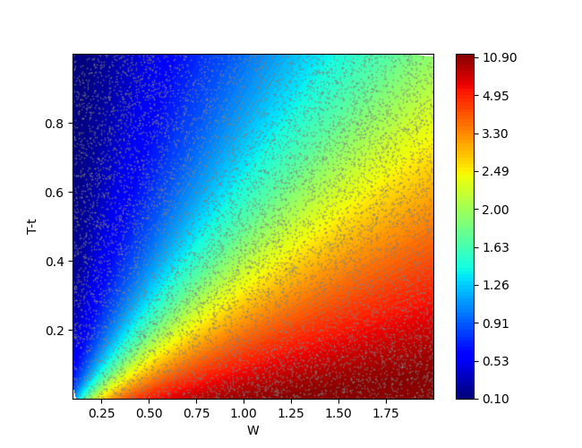
(b) Exact consumption formula

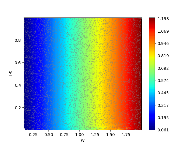
(c) Learned investment policy

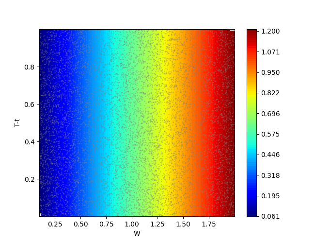
(d) Exact investment formula

Figure 1: Neural vs. exact solutions for consumption/investment under the Merton model. The “Learned” plots (left) are from our PG-DPO-Reg run at iteration 100,000; the “Exact” plots (right) show the closed-form Merton solution.

Figure 1 compares the learned policies (after 100k iterations of PG-DPO-Reg) to the known closed-form solution. Despite the additional difficulty introduced by consumption, the proposed method converges closely to the theoretical optimum after sufficient training.

Quantitative Comparisons.

Tables 1 and 2 report results for PG-DPO and PG-DPO-Reg, respectively. We list the relative MSE (consumption / investment) and an average empirical utility at several iteration milestones. Although both methods eventually approach the known optimum, we observe:

• PG-DPO-Reg (with alignment penalty) attains lower consumption/investment MSE at high iteration counts (compare last columns). In particular, the consumption network benefits from an explicit Pontryagin reference.

• The empirical utility values plateau around the same level for both, but PG-DPO-Reg often stabilizes faster despite an ill-conditioned objective.

• Setting penalty weights $(\alpha_{C},\alpha_{\pi})$ too high can slow early progress, whereas too small yields minimal improvement. Our chosen $(10^{-3},10^{-1})$ balanced those trade-offs.

Discussion.

We see that PG-DPO-Reg generally outperforms PG-DPO, particularly in consumption accuracy ($\text{MSE}=3.46\times 10^{-2}$ vs. $9.65\times 10^{-2}$ at iteration 100k) and somewhat in the investment MSE. Both methods converge to a policy whose empirical utility is close to the theoretical maximum, reflecting that the Merton problem’s ill-conditioning can cause utility plateaus even as the policy itself improves. Overall, the alignment penalty (adopting suitably moderate $(\alpha_{C},\alpha_{\pi})$) appears to improve stability and reduce final policy error. This underscores the value of Pontryagin-based guidance in neural RL for continuous-time finance: while a naïve gradient approach (PG-DPO) can eventually reach high accuracy, the explicit suboptimal-adjoint alignment often “nudges” the learning process toward Pontryagin’s solution more effectively.

8 Conclusion

We have proposed a Pontryagin-Guided Direct Policy Optimization (PG-DPO) framework for Merton’s portfolio problem (Section 5), blending neural-network–based gradient methods with the adjoint (costate) perspective from Pontryagin’s Maximum Principle (PMP). By parametrizing both consumption and investment policies within neural networks and aligning each gradient step to approximate the continuous-time adjoint, our approach balances theoretical rigor with practical flexibility.

A central design choice is to handle the entire time–wealth domain by defining an extended value function over random initial nodes $(t_{0},x_{0})$. This domain-aware sampling allows the policy to learn a truly global solution rather than overfitting to a single initial state. After discretizing only the local sub-interval from $t_{0}$ to $T$, we apply single-path or mini-batch simulation to obtain unbiased gradient estimates, ensuring that the learned policy covers a broad region of $[0,T]\times(0,\infty)$.

In addition, we introduce an adjoint-based alignment penalty that softly regularizes the policy toward Pontryagin’s local controls. Numerical experiments (Section 7) confirm that including this penalty can substantially improve stability and reduce final policy errors, despite the extra cost of a second autodiff pass to retrieve the suboptimal adjoint variables $\lambda_{t}$ and $\partial_{x}\lambda_{t}$. Our results on the Merton problem with consumption show that the alignment-penalty variant (PG-DPO-Reg) outperforms the basic scheme (PG-DPO) in terms of convergence speed and accuracy, while both ultimately reach near-optimal empirical utilities.

Although we do not guarantee global optimality in the high-dimensional neural-parameter space, the strict concavity of the Merton objective ensures a unique global optimum in continuous time. Empirically, the extended domain and alignment penalty help guide parameter updates more reliably toward this Pontryagin-aligned solution, even in the presence of non-convexities. Further refinements could explore advanced variance-reduction techniques, expand to higher-dimensional or constrained markets, or combine value-based PDE elements with the adjoint-based perspective. Overall, these findings illustrate how continuous-time control principles can enrich modern deep learning approaches to stochastic optimization. By embedding the local costate viewpoint into a discrete-time training loop, the PG-DPO framework provides an efficient path to near-optimal controls for complex continuous-time finance problems and beyond.

References

- Beck et al., (2019) Beck, C., E, W., & Jentzen, A. (2019). Machine learning approximation algorithms for high-dimensional fully nonlinear partial differential equations and second-order backward stochastic differential equations. Journal of Nonlinear Science, 29, 1563–1619.
- Becker et al., (2019) Becker, S., Cheridito, P., & Jentzen, A. (2019). Deep optimal stopping. Journal of Machine Learning Research, 20(74), 1–25.
- Borkar, (2008) Borkar, V. S. (2008). Stochastic Approximation: A Dynamical Systems Viewpoint. Cambridge: Cambridge University Press.
- Buehler et al., (2019) Buehler, H., Gonon, L., Teichmann, J., & Wood, B. (2019). Deep hedging. Quantitative Finance, 19(8), 1271–1291.
- Choromanska et al., (2015) Choromanska, A., Henaff, M., Mathieu, M., Arous, G. B., & LeCun, Y. (2015). The loss surfaces of multilayer networks. In Artificial intelligence and statistics (pp. 192–204).: PMLR.
- Dai et al., (2023) Dai, M., Dong, Y., Jia, Y., & Zhou, X. Y. (2023). Learning merton’s strategies in an incomplete market: Recursive entropy regularization and biased gaussian exploration. arXiv preprint arXiv:2312.11797.
- Fleming & Soner, (2006) Fleming, W. H. & Soner, H. M. (2006). Controlled Markov processes and viscosity solutions, volume 25. Springer Science & Business Media.
- Goodfellow, (2016) Goodfellow, I. (2016). Deep learning.
- Gunzburger, (2002) Gunzburger, M. D. (2002). Perspectives in flow control and optimization. SIAM.
- Han & E, (2016) Han, J. & E, W. (2016). Deep learning approximation for stochastic control problems. arXiv preprint arXiv:1611.07422.
- Han et al., (2018) Han, J., Jentzen, A., & E, W. (2018). Solving high-dimensional partial differential equations using deep learning. Proceedings of the National Academy of Sciences, 115(34), 8505–8510.
- Hinze et al., (2008) Hinze, M., Pinnau, R., Ulbrich, M., & Ulbrich, S. (2008). Optimization with PDE constraints, volume 23. Springer Science & Business Media.
- Huré et al., (2020) Huré, C., Pham, H., & Warin, X. (2020). Deep backward schemes for high-dimensional nonlinear pdes. Mathematics of Computation, 89(324), 1547–1579.
- Karatzas & Shreve, (1998) Karatzas, I. & Shreve, S. E. (1998). Methods of Mathematical Finance. New York: Springer.
- Kushner & Yin, (2003) Kushner, H. J. & Yin, G. G. (2003). Stochastic Approximation and Recursive Algorithms and Applications. New York: Springer Science & Business Media.
- Ma & Yong, (1999) Ma, J. & Yong, J. (1999). Forward-backward stochastic differential equations and their applications. Number 1702. Springer Science & Business Media.
- Merton, (1971) Merton, R. C. (1971). Optimum consumption and portfolio rules in a continuous-time model. Journal of Economic Theory, 3(4), 373–413.
- (18) Pardoux, E. & Peng, S. (1990a). Adapted solution of a backward stochastic differential equation. Systems & control letters, 14(1), 55–61.
- (19) Pardoux, E. & Peng, S. (1990b). Adapted solution of a backward stochastic differential equation. Systems & control letters, 14(1), 55–61.
- Pham, (2009) Pham, H. (2009). Continuous-time stochastic control and optimization with financial applications, volume 61. Springer Science & Business Media.
- Pontryagin, (2018) Pontryagin, L. S. (2018). Mathematical theory of optimal processes. Routledge.
- Raissi et al., (2019) Raissi, M., Perdikaris, P., & Karniadakis, G. E. (2019). Physics-informed neural networks: A deep learning framework for solving forward and inverse problems involving nonlinear partial differential equations. Journal of Computational physics, 378, 686–707.
- Reppen & Soner, (2023) Reppen, A. M. & Soner, H. M. (2023). Deep empirical risk minimization in finance: Looking into the future. Mathematical Finance, 33(1), 116–145.
- Reppen et al., (2023) Reppen, A. M., Soner, H. M., & Tissot-Daguette, V. (2023). Deep stochastic optimization in finance. Digital Finance, 5(1), 91–111.
- Ross et al., (2011) Ross, S., Gordon, G., & Bagnell, D. (2011). A reduction of imitation learning and structured prediction to no-regret online learning. In Proceedings of the fourteenth international conference on artificial intelligence and statistics (pp. 627–635).: JMLR Workshop and Conference Proceedings.
- Weinan, (2017) Weinan, E. (2017). A proposal on machine learning via dynamical systems. Communications in Mathematics and Statistics, 1(5), 1–11.
- Yong & Zhou, (1999) Yong, J. & Zhou, X. Y. (1999). Stochastic Controls: Hamiltonian Systems and HJB Equations. New York: Springer.
- Yong & Zhou, (2012) Yong, J. & Zhou, X. Y. (2012). Stochastic controls: Hamiltonian systems and HJB equations, volume 43. Springer Science & Business Media.
- Zhang & Zhou, (2019) Zhang, W. & Zhou, C. (2019). Deep learning algorithm to solve portfolio management with proportional transaction cost. In 2019 IEEE Conference on Computational Intelligence for Financial Engineering & Economics (CIFEr) (pp. 1–10).: IEEE.