Bond-Network Entropy Governs Heat Transport in Coordination-Disordered Solids

Abstract

Understanding how the vibrational and thermal properties of solids are influenced by atomistic structural disorder is of fundamental scientific interest, and paramount to designing materials for next-generation energy technologies. While several studies indicate that structural disorder strongly influences the thermal conductivity, the fundamental physics governing the disorder-conductivity relation remains elusive. Here we show that order-of-magnitude, disorder-induced variations of conductivity in network solids can be predicted from a ‘bond-network’ entropy, an atomistic structural descriptor that quantifies heterogeneity in the topology of the atomic-bond network. We employ the Wigner formulation of thermal transport to demonstrate the existence of a relation between the bond-network entropy, and observables such as smoothness of the vibrational density of states (VDOS) and macroscopic conductivity. We also show that the smoothing of the VDOS encodes information about the thermal resistance induced by disorder, and can be directly related to phenomenological models for phonon-disorder scattering based on the semiclassical Peierls-Boltzmann equation. Our findings rationalize the conductivity variations of disordered carbon polymorphs ranging from nanoporous electrodes to defective graphite used as a moderator in nuclear reactors.

I Introduction

Carbon forms a variety of disordered allotropes useful in several industrial applications: amorphous carbon is a promising material for next-generation electronic and mechanical technologies due to its disorder-tunable electrical conductivity [1], high elastic modulus and hardness [2]; nanoporous carbon is employed as structural nanomaterial [3], as well as in devices for energy harvesting [4, 5] or water desalination [6, 7]; nuclear-grade defective graphite is used as a moderator in nuclear reactors [8, 9]. This wide range of applications is made possible by the high variability in the macroscopic properties of carbon, which derive from its versatility at the atomic scale, particularly its ability to form chain-like bonds between two atoms, planar (graphite-like) bonds involving three atoms, and tetrahedral (diamond-like) bonds between four atoms. The thermal conductivity is a striking example of such high variability [10, 11], as it can change by more than four orders of magnitude — from the ultralow (< 1 W/mK) conductivity of nanoporous carbon [12] to the ultrahigh (>2000 W/mK) conductivity of graphene [13, 14, 15, 16, 17, 18, 19], graphite [20, 21, 22, 23, 24, 25, 26, 27, 28], and diamond [29, 30]. Past works studied structural disorder and thermal conductivity in specific classes of carbon polymorphs, which include: (i) experiments, e.g., in amorphous carbon [31, 32, 33, 34, 35, 36, 37], graphite with variable degree of irradiation-induced defects [38, 39, 40, 41, 42, 43, 44, 45, 46, 47, 48], and nanoporous carbon with different pore-size distributions [12]; (ii) molecular dynamics (MD) simulations [49], e.g., in amorphous carbon [50, 51, 52, 53, 54, 55, 56], electron-irradiated graphite [9], and nanoporous carbon [54, 57, 56]. However, each of those past studies focused on one (or few) of the aforementioned special classes of carbon polymorphs, without investigating similarities and differences between their atomistic structure and macroscopic conductivity. As a result, the structure-conductivity relation is far from being fully understood.

Here, we address this long-standing question relying on the Wigner formulation of thermal transport [58, 59, 60] in conjunction with the machine-learned Gaussian Approximation Potential (GAP) [61]. We employ the latter to describe with quantitative accuracy structural, vibrational, and thermal properties of 23 disordered carbon polymorphs belonging to five different classes: amorphous, irradiated, phase separated, variable porosity, and nanoporous Carbide-Derived Carbon. We find that disorder in the atomic bond network induces order-of-magnitude variations in the thermal conductivity. To quantify such disorder and its relation with conductivity, we decompose the solid into a collection of local atomic environments (LAEs), and we show that in carbon these can be comprehensively characterized using the $H_{1}$ barcode — a ring-based structural descriptor which is formally defined in terms of the first homology group [62]. After discussing how the size (i.e., number of atoms $n$) in the LAE determines the resolution with which structural heterogeneity can be resolved, we define a bond-network entropy (BNE) that, in the presence of disorder, grows with LAE’s size $n$. We demonstrate that the BNE’s growth rate with $n$ quantifies disorder in the atomic bond network, distinguishing the disordered phases of carbon. Most importantly, we rely on these insights to elucidate how disorder affects observables such as the smoothness of the vibrational density of states (VDOS) and the macroscopic thermal conductivity. Finally, we rationalize the physics underlying the correlation between BNE and conductivity by formally connecting the disorder-induced repulsion between vibrational eigenstates to the thermal resistance caused by disorder. Specifically, from the smoothness of the VDOS and diffusivity, we determine the transport lengthscales for all vibrational excitations in irradiated graphite, showing that the characterization of transport lengthscales is not limited to low-frequency modes that approximatively display a band structure blurred by disorder — i.e., a dynamical structure factor (DSF), reminiscent of three acoustic bands with disorder-dependent linewidth [63, 64, 52, 65]. Ultimately, we elucidate the disorder-conductivity relation across a comprehensive range of disordered carbon polymorphs, paving the way for the theory-driven optimization of technologies ranging from nanoporous-carbon-based supercapacitors to moderators for nuclear reactors.

II Wigner formulation of thermal transport

To investigate the atomistic physics underlying the conductivity of disordered carbon, we employ the Wigner Transport Equation [59] (WTE). Such an equation accounts for the quantum Bose-Einstein statistics of vibrations, anharmonicity, and disorder; its solution yields a thermal conductivity expression that comprehensively describes solids ranging from crystals to glasses [60, 66]. In the following we employ the regularized WTE conductivity expression [60] to ensure a proper bulk-limit extrapolation in the presence of disorder:

$$\begin{split}\kappa{=}\frac{1}{\mathcal{V}{N_{\rm c}}}{\sum_{\bm{q},s,s^{\prime}}}&\!\frac{\omega_{\bm{q}s}{+}\omega_{\bm{q}s^{\prime}}}{4}\!\left(\frac{C_{\bm{q}s}}{\omega_{\bm{q}s}}{+}\frac{C_{\bm{q}s^{\prime}}}{\omega_{\bm{q}s^{\prime}}}\right)\!\frac{\rVert\bm{\mathsfit{v}}(\bm{q})_{s,s^{\prime}}\lVert^{2}}{3}\\ \times&\pi\mathcal{F}_{[\eta;\Gamma_{\bm{q}s}{+}\Gamma_{\bm{q}s^{\prime}}]}(\omega_{\bm{q}s}-\omega_{\bm{q}s^{\prime}})\;,\end{split}$$ (1)

where $\mathcal{V}$ is the volume of the reference cell of the solid, $s$ is a mode index and $\bm{q}$ is a wavevector that labels vibrations — the necessity to consider $\bm{q}$ depends on the size and degree of disorder in the solid, for strongly disordered systems described with very large ($\gtrsim 5000$ atoms) reference cell, it is sufficient to consider only $\bm{q}{=}\bm{0}$ [67, 60] (more on this later). $\omega_{\bm{q}s}$ and $C_{\bm{q}s}$ are the frequency and the quantum specific heat of the vibration $\bm{q}s$:

$$C_{\bm{q}s}=C[\omega_{\bm{q}s},T]=\frac{\hbar^{2}\omega_{\bm{q}s}^{2}}{k_{\rm B}T^{2}}\mathsfit{N}_{\bm{q}s}(\mathsfit{N}_{\bm{q}s}+1),$$ (2)

where $\mathsfit{N}_{\bm{q}s}$ is the Bose-Einstein distribution at temperature $T$: $\mathsfit{N}_{\bm{q}s}=[\exp{(\hbar\omega_{\bm{q}s}/k_{\rm B}T)}-1]^{-1}$. $\bm{\mathsfit{v}}(\bm{q})_{s,s^{\prime}}$ is the velocity operator — its diagonal elements are the usual group velocities, while its off-diagonal non-degenerate elements describe couplings between different vibrations. $\mathcal{F}_{[\eta;\Gamma_{\bm{q}s}{+}\Gamma_{\bm{q}s^{\prime}}]}$ is a two-parameter Voigt distribution, employed to numerically preserve in finite-size models of disordered solids the physical property that neighbouring (quasi-degenerate) vibrational modes can interact and conduct heat even in the limit of vanishing intrinsic linewidths $\Gamma_{\bm{q}s}$ (due to third-order anharmonic interactions and isotope-mass impurities). Specifically, $\eta$ is a computational parameter that has to be numerically converged [60, 67] and is of the order of the average energy-level spacings, see Supplementary Materials (SM) for details. When $\Gamma_{\bm{q}s}{+}\Gamma_{\bm{q}s^{\prime}}{\gg}\eta$, the Voigt distribution reduces to a Lorentzian $L[\omega,\Gamma]=\frac{1}{\pi}\frac{\Gamma/2}{\omega^{2}+(\Gamma/2)^{2}}$ with full width at half maximum (FWHM) $\Gamma$ determined by the sum of the intrinsic linewidths of mode $\bm{q}s$ and $\bm{q}s^{\prime}$, while in the opposite limit $\Gamma_{\bm{q}s}{+}\Gamma_{\bm{q}s^{\prime}}{\ll}\eta$ it reduces to the Gaussian representation of the Dirac delta. In formulas,

$$\mathcal{F}_{[\eta;\Gamma_{\bm{q}s}{+}\Gamma_{\bm{q}s^{\prime}}]}{\rightarrow}\begin{cases}L[\omega_{\bm{q}s}{-}\omega_{\bm{q}s^{\prime}},\!\Gamma_{\bm{q}s}{+}\Gamma_{\bm{q}s^{\prime}}],\rm{for}\;\Gamma_{\bm{q}s}{+}\Gamma_{\bm{q}s^{\prime}}\gg\eta\\ \frac{1}{\pi\eta}\exp{(-\frac{1}{\pi}\frac{(\omega_{\bm{q}s}-\omega_{\bm{q}s^{\prime}})^{2}}{\eta^{2}})},\rm{for}\;\Gamma_{\bm{q}s}{+}\Gamma_{\bm{q}s^{\prime}}\ll\eta\end{cases}$$ (3)

Eq. (3) implies that: for $\Gamma_{\bm{q}s}{+}\Gamma_{\bm{q}s^{\prime}}{\gg}\eta$ Eq. (1) yields the standard anharmonic WTE conductivity [59], while in the opposite limit $\Gamma_{\bm{q}s}{+}\Gamma_{\bm{q}s^{\prime}}{\ll}\eta$ Eq. (1) numerically reduces to the harmonic Allen-Feldman (AF) [68] conductivity.

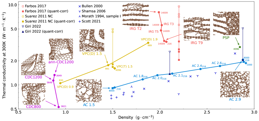
Figure 1: Room-temperature conductivity as a function of density in various classes of carbon polymorphs. Carbide-derived carbon (CDC) is purple, variable-porosity carbon (VPC) is yellow, amorphous carbon (AC) is blue, irradiated graphite (IRG) is red, and phase-separated phase (PSP) is green. Filled markers are results from this work, empty markers are direct results from MD simulations (irradiated graphite from Farbos et al. [9], nanoporous carbon from Suarez-Martinez and Marks [54], Amorphous Carbon from Giri et al. [50]). The filled markers connected by lines to empty markers are results from classical MD simulations [9, 54, 50] corrected to account for the quantum Bose-Einstein statistics of vibrations (see Appendix A for details). The unfilled markers x, +, , are experiments in amorphous carbon [33, 34, 31, 35]. Next to the conductivity values, we report the names of the structures and the number of atoms in their simulation cells.

III Conductivity of disordered carbon polymorphs

Fig. 1 shows the room-temperature conductivity of five structurally different classes of carbon polymorphs, obtained evaluating Eq. (1) with the quantum-accurate GAP potential [61]. In particular, carbide-derived carbon (CDC) is a low-density ($\leq 1.0$ g/cm³) solid consisting of nanoporous, curved graphene sheets with tunable amount of coordination defects. CDC draws its name from the carbide precursors (TiC or SiC) used in the chlorination-based synthesis procedure [69, 12]; its properties depend on the chlorination temperature, which is therefore reported in the structure name [69] (e.g., CDC800 and CDC1200 refer to materials synthesized with a chlorination temperature of 800 and 1200 ^∘C, respectively, and ann-CDC1200 denotes a CDC1200 structure further annealed after synthesis, see SM). Variable-porosity carbon (VPC) is constituted of curved graphene sheets with variable porosity and rare coordination defects; their density ranges from 0.9 to 1.9 g/cm³ [70, 71, 54]. Amorphous carbon (AC) is a packed structure with variable density from 1.5 to 3.5 g/cm³, where atoms have coordination number that ranges from two to four and its average increases with density [33, 34, 50, 52, 56]. Irradiated graphite (IRG) features inter-layer bonding defects (interstitial atoms, dislocations, and point defects) caused by electron or neutron irradiation, in concentration proportional to the irradiation time [9]. Finally, the phase-separated phase (PSP) structure blends a mostly 3-fold coordinated graphitic phase with a mostly 4-fold coordinated amorphous-carbon phase [71].

The room-temperature conductivity of these polymorphs varies by more than one order of magnitude, from 0.5 W/mK for CDC800 to 8.1 W/mK for IRG with the lowest irradiation time (‘IRG T2’ corresponds to an exposure to irradiation of 2 min). Notably, we find that the thermal conductivity-density relation highly depends on the type of disorder. For AC and VPC, increasing density causes an increase in conductivity, which is faster in VPC compared to AC (the former shows 69$\%$ decrease in $\kappa$ upon decreasing density from 1.9 to 0.9 g/cm³, while the latter shows 56$\%$ decrease in $\kappa$ upon decreasing density from 2.9 to 1.5 g/cm³). In CDC, the structural details — determined by the chlorination temperature used in the synthesis [69] — have a weak (negligible) influence on the density but strongly impact the thermal conductivity, which decreases by 53% upon decreasing the chlorination temperature from 1200 to 800 ^∘C. Similar conductivity variations at nearly constant density are observed in IRG structures, where increasing the irradiation exposure from 2 to 9 min causes a conductivity reduction of $56\%$. Lastly, we see that annealing the maximum-density AC phase (2.9 g/cm³) yields partial graphitization (PSP phase) and a conductivity increase of 44$\%$.

Fig. 1 also shows that our nanometric atomistic models are sufficiently large to describe the bulk limit of the conductivity [72, 60, 67, 64, 73, 63]; in fact, for all the polymorphs, we studied multiple atomistic models of sizes differing by more than one order of magnitude, and always found compatible results for their conductivity. Importantly, we highlight that our conductivity predictions are broadly compatible in trend and magnitude with several independently performed experiments and simulations. For example, in AC our conductivities are compatible with: (i) experiments by Bullen et al. [33], Shamsa et al. [34], Morath et al. [31] and Scott et al. [35]; (ii) MD simulations by Giri et al. [50], after accounting for quantum corrections [74] (see Appendix A for details). Using analogous quantum corrections, our predictions for VPCs at density 1.5 g/cm³ are in agreement with those from Ref. [54] — specifically, we note that the proportions of three-coordinated atoms in the two structures we considered from Ref. [54] (95.1% and 98.3%, respectively) are close to those in our work (96.5% for VPC(D), and 97.6 % for VPC(T)). For IRG, the conductivity dependence on irradiation agrees with previous MD results [9]. In CDC, the increase of thermal conductivity with chlorination temperature agrees with the experimentally observed trend [12]. Finally, we note that the analysis above has been limited to room temperature because this is sufficient for our goal of understanding the disorder-conductivity relation; the temperature dependence of the conductivity is discussed in detail in SM.

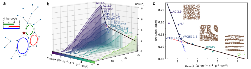
Figure 2: Relation between bond-network entropy and thermal conductivity in disordered carbon. Panel a, $H_{1}$ barcode of an exemplary local atomic environment (LAE) around an atom (red star) in amorphous carbon with size $n=23$. Panel b, Growth of the bond-network entropy with the size of LAEs ordered by their value of room-temperature conductivity divided by density. Panel c, Relation between average value of bond-network entropy divided by size of LAEs, ${\rm BNE}(n)/n$, and room-temperature conductivity divided by density, $\kappa_{\rm 300K}/\rho$. Dashed red and blue lines are linear regression fits on the subsets of the data $\kappa_{\rm 300K}/\rho$ larger or smaller than 1.5 $\text{W}\!\cdot\!\text{m}^{-1}\!\cdot\!\text{K}^{-1}\!\cdot\!\text{g}^{-1}\!\cdot\!\text{cm}^{3}$, respectively, the black line is their smooth interpolation.

IV Thermal conductivity & bond-network entropy

To characterize the disorder-conductivity relation, we introduce a descriptor of disorder that quantifies heterogeneity in the atomic bond network. The salient idea is to represent a solid as a collection of local atomic environments (LAEs) sampled from a certain probability distribution — for a perfect crystal, this distribution will be peaked only around environments contained in crystal’s primitive cell, while for a disordered solid the number of different LAEs will be higher and therefore their distribution broader. We start by defining a LAE around a reference atom by constructing a connection graph that starts from such reference atom and reaches its $n-1$ closest neighbours, with $n$ denoting the size of the LAE. We consider atoms as graph vertices, which are connected if they are within the carbon bonding distance (1.8 Å). We distinguish between different LAEs by looking at their ring structure; specifically, we employ the $H_{1}$ barcode descriptor [62] to characterize the algebraically independent rings in the LAE. For example, the LAE in Fig. 2a contains three algebraically independent rings (green, red and blue), which are classified by $H_{1}$ barcode in terms of their minimum and maximum edge distance from the reference-atom vertex (0-2 for green, 1-3 for red, and 0-3 for blue); see Appendix B for technical details. Changing the LAE’s size $n$ allows us to change the resolution with which we resolve structural disorder in a solid. For small values of $n$ (e.g., $n\lesssim 4$) the LAE contains information only about connectivity between nearest neighbours, and therefore describes short-range order (SRO). For $14{\lesssim}n{\lesssim}30$, the LAEs are large enough to describe structural features in the lengthscale range 5-20Å, known as medium-range order (MRO) [75].

To describe disorder through the statistical distribution of LAEs, for each atom in our system we consider an $n$-sized LAE centered around it, we calculate its $H_{1}$ barcode (one for each atom in the system) and construct a distribution of $H_{1}$ barcodes:

$$P(H_{1},n)=\frac{1}{N_{\rm at}}\sum_{b}\delta_{H_{1}[{\rm LAE}(b,n)],H_{1}},$$ (4)

where $N_{\rm at}$ is the number of atoms in the atomistic model, $H_{1}[\rm{LAE}(b,n)]$ is the $H_{1}$ barcode of the LAE having size $n$ and centered at atom $b$, and $\delta_{H_{1}[{\rm LAE}(b,n)],H_{1}}$ is an indicator function equal to one if $H_{1}[{\rm LAE}(b,n)]$ is equal to the given barcode $H_{1}$, and zero otherwise. The $H_{1}$ barcode distribution (4) becomes broader as disorder in the topology of the atomic bond network increases. Therefore, it is natural to quantify disorder through the information entropy of such a distribution, which we will hereafter intuitively refer to as bond-network entropy (BNE):

$${\rm BNE}(n)=-\sum_{H_{1}}P(H_{1},n)\ln{P(H_{1},n)}.$$ (5)

To understand the information provided by BNE, it is useful to evaluate it in two limiting cases: (i) a perfectly ordered, idealized crystal with one atom per primitive cell; (ii) a strongly disordered bulk glass. In the idealized crystalline case BNE$(n){=}0\;\forall\;n$, since the crystal order implies that each atom in the system has the same LAE for all $n$, and therefore $P(H_{1},n)$ is a Kronecker delta. In contrast, in the second case, we find that the presence of disorder yields the following behavior: (i) for $n$ sufficiently large to capture disorder, different atoms have different barcodes and hence BNE$(n){>}0$; (ii) due to the presence of disorder, upon increasing $n$ more algebraically independent rings are found, and hence BNE grows with the LAE’s size $n$.

A key finding of this work is that the growth rate of BNE($n$) is determined by the degree of disorder in the topology of the atomic bond network — Fig. 2b shows that BNE’s growth rate can be used to distinguish different classes of carbon polymorphs. In particular, BNE($n$) displays the fastest growth with $n$ in the phases having the lowest conductivity (e.g., AC and CDC800). As disorder decreases, the growth rate becomes lower: a medium growth rate is found for CDC1200, VPC(D) 1.5 or IRG T9, and the lowest growth rate emerges in weakly irradiated graphite (IRG T3 and T2). We note, in passing, that the atomistic models discussed here have a size much larger than the range of LAE’s size $n$ reported in Fig. 2; therefore this analysis is not affected by periodic boundary conditions (see Fig. 7 in Appendix C for details). In Fig. 2c we show that BNE’s average growth rate (computed averaging ${\rm BNE}(n)/n$ for $n\in[14,30]$) and room-temperature conductivity divided by density are inversely correlated (Spearman’s rank-correlation coefficient equal to -0.947). For the materials analyzed here the correlation is approximatively piecewise linear, with two different slopes characterizing (weakly disordered) irradiated graphite and (strongly disordered) amorphous structures; CDC1200, ann-CDC1200 and VPC nanoporous carbons are in the smooth-crossover region between them. The correlation in Fig. 2c provides insights on the influence of atomic disorder on the conductivities in Fig. 1. Starting from a comparison between AC and VPC at density 1.5 g/cm³, we rationalize the lower conductivity of the former as originating from a higher degree of disorder in the bond network (i.e., higher BNE($n$) for $n{\in}[14,30]$). Analogous considerations hold for CDC and IRG, where samples with very similar density show conductivities that are very different and inversely related to BNE($n$). Focusing on the conductivity variations observed within a certain family upon changing density, we see that in AC, increasing density from 1.5 to 2.9 g/cm³ has negligible effect on BNE($n$); therefore, the conductivity differences between the various phases of AC can be explained mainly in terms of density — we will see later that the higher the density, the higher the number of vibrational modes per unit volume, and in disordered systems this contributes to increasing the conductivity. In contrast, in VPC increasing density implies also a decrease in disorder (BNE($n$)); therefore, the conductivity increase observed in VPC upon increasing density is stronger than in AC. Overall, these findings suggest that conductivity and density measurements can be used to quantify the structural heterogeneity of disordered solids, and motivate us to investigate the relationship between the structural-disorder descriptor BNE and both thermal and vibrational properties.

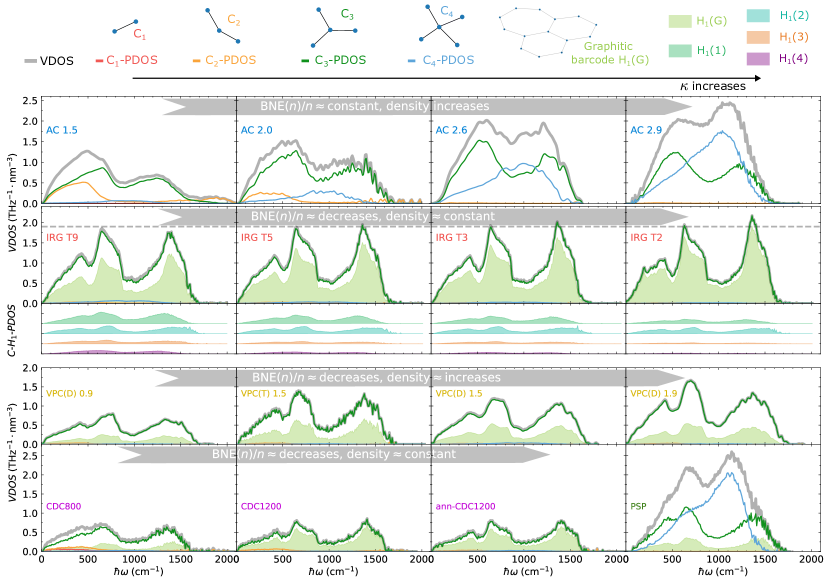
Figure 3: Dependence of VDOS on short- and medium-range order. The panels are split by different groups of structures: first row is AC, second row is IRG, third row is VPC, and fourth row shows CDC & PSP. The total VDOS is thick gray, its decomposition into $C$-PDOS contributions from atoms having different coordination (SRO) is given by thin lines of different colors: red for dangling bonds (present only in AC 1.5 and CDC800, albeit practically invisible), while orange, green, and blue show the PDOS for two-, three-, and four-fold coordinated atoms, respectively. The shaded areas show the $C_{3}$-$H_{1}$-PDOS: light green corresponds to the graphitic barcode, and the other four colors show other common barcodes in IRG. The dashed gray horizontal line in the IRG panel shows that the VDOS becomes smoother as irradiation-induced structural disorder increases.

V Atomic vibrations & bond-network entropy

In this section we show that a relation between BNE and microscopic vibrational properties exists. We start by characterizing atomic vibrations with the VDOS:

$$g(\omega)=\frac{1}{\mathcal{V}N_{\rm c}}\sum_{{\bm{q},s}}\delta(\omega-\omega_{\bm{q}s}).$$ (6)

We also resolve how atoms with a certain coordination contribute to the VDOS by decomposing Eq. (6) into coordination-resolved partial VDOS [76, 67] ($C$-PDOS),

$$g_{C_{x}}(\omega)=\frac{1}{\mathcal{V}N_{\rm c}}\sum_{{\bm{q},s}}\delta(\omega-\omega_{\bm{q}s})\sum_{b,\alpha}|\mathcal{E}^{b\alpha}_{{\bm{q}s}}|^{2}\delta_{b,C_{x}},$$ (7)

where $\delta_{b,C_{x}}$ is an indicator function equal to one if atom $b$ has coordination number equal to $x$, and zero otherwise; $\mathcal{E}^{b\alpha}_{{\bm{q}s}}$ is the eigendisplacement that describes how atom $b$ oscillates in direction $\alpha$ when the mode $\bm{q}s$ is excited [77, 59]. Eq. (7) is directly related to the VDOS via marginalization over the coordination variable: $\sum_{C_{x}}g_{C_{x}}(\omega){=}g(\omega)$. Importantly, we can go beyond the SRO nearest-neighbour (coordination) analysis and look at how MRO properties influence the VDOS. To this aim, we further decompose the $C$-PDOS into contributions from different $H_{1}$ barcodes ($C$-$H_{1}$-PDOS):

$$\begin{split}&g_{C_{x},H_{1}}(\omega)=\\ &\frac{1}{\mathcal{V}N_{\rm c}}\sum_{{\bm{q},s}}\delta(\omega-\omega_{\bm{q}s})\sum_{b,\alpha}|\mathcal{E}^{b\alpha}_{{\bm{q}s}}|^{2}\delta_{b,C_{x}}\delta_{H_{1}[{\rm LAE}(b,n)],H_{1}},\end{split}$$ (8)

where we choose the size of the LAE $n$ to be equal to 14 for the following reasons: (i) $n=14$ is sufficiently large to capture changes in the MRO features related to 3 graphitic 6-fold rings, even in the presence of perturbations in the graphite interlayer distance, or changes in the number of atoms within one of the rings; (ii) the range $n\in[14,30]$ is sufficient to capture signatures of MRO, and since Fig. 2 shows that the BNE’s growth with $n$ is practically constant for $n\in[14,30]$, we can choose the lowest value of $n$. Finally, it can be verified that marginalizing the $C$-$H_{1}$-PDOS (8) with respect to the barcode variable yields the $C$-PDOS (7): $\sum_{H_{1}}g_{C_{x},H_{1}}(\omega)=g_{C_{x}}(\omega)$.

In Fig. 3 we plot the VDOS and its decomposition into $C$-PDOS and $C$-$H_{1}$-PDOS for all the families of carbon polymorphs studied. Starting from AC, we see that increasing density yields an increase in magnitude of the VDOS, which trivially follows from the appearance of the system’s cell volume $\mathcal{V}$ in the denominator of Eq. (6). Moreover, the changes in the shape of the VDOS with density are determined by having different proportions of $C_{2}$, $C_{3}$ and $C_{4}$ coordination environments, and we highlight how the shape of the $C$-PDOS contributions are almost unchanged across all amorphous carbon structures (see Fig. SF 2 in SM for details). In particular, at low density (1.5 g/cm³) the VDOS is bimodal with the low-frequency peak stronger than the high-frequency peak — the $C$-PDOS decomposition shows that these are determined by a superimposition of a monomodal low-frequency $C_{2}$ PDOS and a bimodal $C_{3}$ PDOS. Upon increasing density, the magnitude of the low-frequency monomodal $C_{2}$ contribution is progressively replaced by a high-frequency monomodal $C_{4}$ PDOS, resulting in a bimodal distribution with the high-frequency peak stronger than the low-frequency peak. In contrast, in less disordered polymorphs such as CDC, VPC and IRG, SRO is dominated by the $C_{3}$ coordination environment, hence VDOS $\approx C_{3}$-PDOS — this indicates that these solids are ordered over the SRO lengthscale, and therefore the visible VDOS changes must originate from disorder over a larger lengthscale. Therefore, in Fig. 3 we further decompose the $C_{3}$-PDOS into contributions from different MRO using the $C_{3}$-$H_{1}$-PDOS. We show that the ‘graphitic $H_{1}(G)$’ barcode — which describes MRO due to three hexagonal 6-fold rings — allows us to resolve whether the $C_{3}$ SRO is associated with high density of graphitic rings (e.g., CDC1200 and IRG-T2) or not (e.g., CDC800). We note, in passing, that the $C_{3}$-$H_{1}(G)$-PDOS has a triple-modal shape in all IRG structures, as well as in CDC1200 and in medium-high density VPC — specifically, we show in the SM Fig. SF 3 that for a finite concentration of graphitic $H_{1}(G)$ environments, the shape of $C_{3}$-$H_{1}(G)$-PDOS is practically independent from their concentration. More generally, the decomposition of IRG’s $C_{3}$-PDOS into the five most frequent barcodes (shaded areas in Fig. 3) shows that increasing disorder yields an increase in the number of different barcodes at a fixed LAE size that contribute to the VDOS, consistently with BNE’s increase shown in Fig. 2. Most importantly, we note that different barcode environments have $C_{3}$-$H_{1}$-PDOS with different shapes; their superimposition leads to an overall smoothing of the VDOS, and hence a decrease in the magnitude of its peaks. These findings generally apply to all carbon polymorphs, as we observe VDOS smoothing when we compare: (i) CDC1200 and CDC800; (ii) VPC(D) 1.9, 1.5, and 0.9; (iii) PSP and AC 2.9. In summary, increasing disorder in the atomic bond network causes an increase in BNE’s growth rate and in the VDOS’ smoothness; in the next section we show that the latter can be related to Kittel’s empirical model for phonon scattering due to structural disorder [78].

VI Explicitly Disordered Glass vs Perturbatively Disordered Crystal

In this section we elucidate a relation between our WTE-based conductivity predictions and those obtained employing Kittel’s phenomenological treatment of the thermal resistance induced by disorder [78, 79]. We will show how this relation allows us to connect BNE, smoothness of the VDOS, and conductivity to the lengthscales of disorder and of the heat-transport mechanisms, thus fundamentally rationalize the correlation between BNE and thermal conductivity shown in Fig. 2.

We start by resolving the thermal conductivity with the usual frequency-dependent decomposition [60]

$$\kappa=\int_{0}^{\omega_{\rm max}}d\omega\,g(\omega)C(\omega)D(\omega),$$ (9)

where $\omega_{\rm max}$ is the maximum vibrational frequency of the solid, $g(\omega)$ is the VDOS (6), $C(\omega)$ is the specific heat of a vibration with frequency $\omega$ (Eq. (2)), and $D(\omega)$ is its diffusivity, describing the rate at which the heat carried by a vibration spreads [68]. The first description of heat transport in the presence of structural disorder was done relying on the semiclassical Peierls-Boltzmann transport equation (BTE) [80] and phenomenologically considering disorder-induced thermal resistance in a ‘Perturbatively Disordered Crystal’ (PDC). This description interprets the diffusivity in terms of particle-like excitations having energy $\hbar\omega$ and propagating isotropically with velocities $v_{\rm eff}(\omega)$ over disorder-limited transport lengthscales (mean free paths) $\lambda_{\rm eff}(\omega)$:

$$D_{\rm PDC}(\omega)=v_{\rm eff}(\omega)\lambda_{\rm eff}(\omega)=\frac{v^{2}_{\rm eff}(\omega)}{\Gamma_{\rm dis}(\omega)},$$ (10)

where the last equality follows from the relation $v_{\rm eff}(\omega)/\lambda_{\rm eff}(\omega){=}\Gamma_{\rm dis}(\omega)$, with $\Gamma_{\rm dis}(\omega)$ being the ‘disorder linewidth’ or inverse scattering time $\Gamma_{\rm dis}(\omega){=}[\tau_{\rm dis}(\omega)]^{-1}$ that describes the thermal resistance encountered by a vibration $\omega$ due to the presence of structural disorder.

A well known special case of Eq. (10) is Kittel’s ‘phonon liquid’ picture [78], which attempted to phenomenologically explain the conductivity of glasses by combining the BTE with Casimir’s model [79] for phonon-interface scattering around its physical lower bound. Specifically, this picture considers: (i) the mean free path (MFP) $\lambda_{\rm eff}(\omega)$ to be a frequency-independent lengthscale $\lambda_{\rm eff}(\omega){\to}\Lambda_{0}$ determined by the type disorder (e.g., for silica glass [78] $\Lambda_{0}$ is the ring size ${\approx}7$Å); (ii) the propagation velocity $v_{\rm eff}(\omega)$ as frequency-independent average velocity of sound ($v_{\rm eff}(\omega){\to}v_{\rm sound}$). Kittel’s model is top-down interpretative but not bottom-up predictive; in fact, it allows to estimate the value of the microscopic $\Lambda_{0}$ from the knowledge of measured values of $\kappa$ (as well as of $v_{\rm sound}$ and $C$), but does not provide a rigorous prescription for determining the value of $\Lambda_{0}$ from first principles that can be used for the bottom-up prediction of $\kappa$. To address the limitations of Kittel’s phenomenological explanation, Allen and Feldman [68] (AF) introduced an alternative definition of diffusivity for harmonic glasses based on a Zener-like tunnelling transport mechanism between quasi-degenerate vibrational modes. In contrast to considering disorder as originating from perturbations of long-range crystalline order, AF describes heat transport in an Explicitly Disordered Glass (EDG) that does not need a crystalline precursor, or a relation to it. As already mentioned, the harmonic AF formalism emerges as a special case of the more general anharmonic WTE framework [59], and in the following we show that the latter allows to shed light on the connection between atomic disorder, VDOS smoothing, macroscopic $\kappa$ and Kittel’s phonon liquid interpretation.

We start by showing that the WTE exposes a proportionality relation between the diffusivity of a generic (EDG or PDC) disordered system, its VDOS and quasi-degenerate velocity operator elements ($\bm{\mathsfit{v}}_{s,s^{\prime}}$ with $\omega_{s}{\simeq}\omega_{s^{\prime}}$). This is apparent when we consider Eq. (1) in the EDG limit, i.e.: (i) we take the bulk-disordered limit (in practice using $\mathcal{V}$ containing thousands of atoms and thus considering $\bm{q}{=}\bm{0}$ only); (ii) we consider linewidths slowly varying with frequency, larger than the average energy-level spacing, and far from the overdamped regime. This implies that the Voigt distribution reduces to a Lorentzian with FWHM determined by the sum of intrinsic linewidths $\Gamma_{s}{+}\Gamma_{s^{\prime}}$ of vibrations with practically equal frequencies $\omega_{s}{\sim}\omega_{s^{\prime}}$ and specific heats $C_{s}{\sim}C_{s^{\prime}}$. Under these conditions, the WTE diffusivity [60] reduces to:

$$\begin{split}D_{\rm EDG}(\omega)\!&=\!\frac{\pi}{\mathcal{V}g(\omega)}\!\sum_{s,s^{\prime}}\!\frac{\rVert\bm{\mathsfit{v}}_{ss^{\prime}}\lVert^{2}}{3}\!L[\omega_{s}{-}\omega_{s^{\prime}}\!,\Gamma_{s}{+}\Gamma_{s^{\prime}}]\delta(\omega-\omega_{s})\\ &\approx\pi{\Upsilon^{2}(\omega)}\frac{1}{\rho_{n}}\left[\int d\omega^{\prime}L[\omega{-}\omega^{\prime}\!,\Gamma(\omega)]g_{d}(\omega^{\prime})\right],\\ \end{split}$$ (11)

where the simplification from the first to the second line is justified in strongly disordered systems [60, 67] that feature velocity-operator elements negligibly dependent on the frequency difference between the modes $s$ and $s^{\prime}$ (these are denoted by ${\Upsilon^{2}(\omega_{s})}{\approx}N_{\rm at}{\rVert\bm{\mathsfit{v}}_{ss^{\prime}}\lVert^{2}}/{3}$, see Appendix D). Moreover, in the second line we have denoted the atom number density with $\rho_{n}{=}\frac{N_{\rm at}}{\mathcal{V}}$, and rewritten the mode linewidth $\Gamma_{s}$ as a function of frequency $\Gamma(\omega_{s})$ using the bijective mapping between frequency and mode arising from lack of symmetries (and hence lack of perfectly degenerate frequencies) in disordered systems [81]. Eq. (11) shows that in an EDG the diffusivity is practically determined by a convolution between a Lorentzian $L[\omega-\omega^{\prime},\Gamma(\omega)]$ and the ‘dressed’ VDOS

$$\begin{split}g_{d}(\omega)\!=\!\frac{1}{\mathcal{V}}\!\sum_{s}\!L[\omega{-}\omega_{s},\Gamma(\omega_{s})]{=}{\int}{d\omega^{\prime}}L[\omega{-}\omega^{\prime},\Gamma(\omega^{\prime})]g(\omega^{\prime}),\end{split}$$ (12)

whose name derives from its differences relative to the ‘bare’ VDOS $g(\omega)$ defined in Eq. (6). Specifically, within the many-body Green’s function formalism, the Dirac deltas $\delta(\omega{-}\omega_{s})$ appearing in the bare VDOS (6) can be seen as resulting from the integration of bare non-interacting phonon spectral functions, while in the dressed VDOS (12) we have the integration of Lorentzian spectral functions $b(\omega)_{s}{=}\frac{1}{\pi}\!\frac{\Gamma_{s}/2}{(\omega{-}\omega_{s})^{2}{+}(\Gamma_{s}/2)^{2}}$, i.e., $g_{d}(\omega){=}\frac{1}{\mathcal{V}}\sum_{s}b(\omega)_{s}$ [82, 83] where the broadenings $\Gamma_{s}$ are determined by interactions (due to, e.g., disorder or anharmonicity). We highlight that the second equivalence in Eq. (12) shows that the dressed VDOS is related to the ‘bare’ VDOS $g(\omega)$ via a ‘dressing’ integral, which practically is a convolution with a Lorentzian having frequency-dependent broadening (linewidth) and implies that the dressed VDOS becomes smoother as linewidths (proportional to the interaction strength) become larger.

In strongly disordered systems (EDG), the vibrational energy levels significantly repel each other [84], implying that the bare VDOS is already very smooth and practically indistinguishable from the dressed VDOS, $g_{\rm EDG}(\omega)\approx g_{d}(\omega)$. This also implies that we can neglect the convolution between dressed VDOS and Lorentzian in the second line of Eq. (11), obtaining that in this (non-interacting or harmonic) disordered limit the diffusivity of an EDG is directly proportional to the bare VDOS:

$$D_{\rm EDG}(\omega)\approx D_{\rm AF}(\omega)=\pi{\Upsilon^{2}(\omega)}\frac{1}{\rho_{n}}g_{\rm EDG}(\omega).$$ (13)

Eq. (13) shows that the EDG diffusivity arises from a vibration interacting with a dense set of quasi-degenerate vibrations, and the strength of these interactions is described by the square of the quasi-degenerate velocity operator $\Upsilon^{2}(\omega)$. Finally, we note that Eq. (13) can be equivalently obtained from Eq. (11) by taking the ordered limit $\mathcal{V}{\to}\infty$ and $\Gamma_{s}{\to}\eta{\to}0$, and coincides with the AF diffusivity [68].

VII Disorder-induced VDOS smoothing & thermal resistance.

In Kittel’s model for conduction in a PDC, $\kappa$ (Eqs.(9, 10)) is influenced by structural disorder through the phenomenological disorder-limited MFP. In contrast, in the rigorous WTE treatment of an EDG (Eqs.(9, 11)), disorder impacts both VDOS and diffusivity. It is therefore natural to ask whether it is possible to obtain two compatible physical descriptions of heat transport using the rigorous WTE for an EDG and Kittel’s phenomenological treatment for a PDC. Here we demonstrate that this is indeed possible, showing that Kittel’s PDC formula can be derived from the WTE EDG through algebraic manipulations; then, we use these insights to formally determine Kittel’s disorder-limited MFP.

We start by recalling that Kittel’s model assumes specific heat and VDOS to be those of an Unperturbed Ordered Crystal (UOC), and accounts for disorder through a phenomenologically determined PDC diffusivity. Since the WTE in the EDG limit shows that in the presence of structural disorder the diffusivity is related to the VDOS (Eq. (11)), we hypothesize that the unknown Kittel’s PDC diffusivity also assumes such functional form, which we highlight contains a convolution between the dressed VDOS and a Lorentzian distribution having FWHM that is unknown (and in principle frequency-dependent). Importantly, through algebraic manipulations one can recast such convolution to apply on the UOC VDOS appearing at the very beginning of Kittel’s conductivity expression. These manipulations imply that the disorder-mediated interaction that limits thermal transport within Kittel’s model can be formally related to the smoothing of the dressed VDOS. In particular, Kittel’s unknown disorder linewidth $\Gamma_{\rm dis}(\omega)$ in Eq. (10) can be determined as the broadening that within the convolution (Eq. (12)) transforms the bare UOC VDOS into a dressed PDC VDOS equal to the bare EDG VDOS. In formulas:

$$\begin{split}\kappa_{\rm PDC}&=\int d\omega\,g_{\rm UOC}(\omega)C(\omega)D_{\rm unknown}(\omega)\\ &=\int d\omega\,g_{\rm UOC}(\omega)C(\omega)\pi{\Upsilon^{2}(\omega)}\frac{1}{\rho_{n}}\\ &\qquad\qquad\;\times\left[\int d\omega^{\prime}L[\omega{-}\omega^{\prime}\!,\Gamma_{\rm dis}(\omega)]g_{\rm PDC}(\omega^{\prime})\right]\\ &\approx\int d\omega\,\underbrace{g_{\rm PDC}(\omega)}_{\approx g_{\rm EDG}(\omega)}C(\omega)\underbrace{\left[\pi\Upsilon^{2}(\omega)\frac{1}{\rho_{n}}g_{\rm PDC}(\omega)\right]}_{\approx D_{\rm EDG}(\omega)\approx D_{\rm AF}(\omega)},\end{split}$$ (14)

where the last approximated equivalence holds under the assumptions used to obtain Eq. (11) and Eq. (13), see Appendix E for details. From a mathematical viewpoint, Eq. (14) shows that the algebraic manipulations used to rewrite the WTE EDG conductivity in Kittel’s form are self-consistent, i.e. by rearranging the integration of the Lorentzian appearing in the WTE conductivity (1) one obtains an expression in which the dressed PDC VDOS appears twice, consistently with the form of the WTE EDG conductivity (13) (see Appendix E for details).

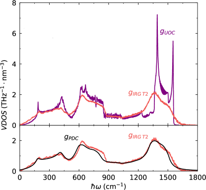
Figure 4: Equivalence map between PDC and EDG. Top, VDOS of unperturbed, ordered crystalline (UOC) graphite (purple) and of EDG irradiated graphite (IRG T2, red). Bottom, PDC VDOS $g_{\rm PDC}(\omega)$ obtained perturbing the VDOS of UOC graphite (black), and VDOS of EDG IRG T2 (red).

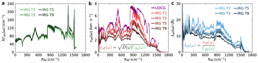
Figure 5: Influence of structural disorder on linewidths (a), propagation velocity (b), and vibrations’ mean free paths (c). Starting from Unperturbed Ordered Crystalline Graphite (UOCG), structural disorder is progressively induced by irradiation in samples IRG T2, T3, T5, and T9 (see text). Increasing disorder yields larger linewidths and lower velocities; consequently, the vibrational mean free paths decrease upon increasing disorder.

In practice, $\Gamma_{\rm dis}(\omega)$ is determined starting from the established [85, 86] frequency-linewidth relations for phonon-disorder scattering,

$$\Gamma_{\rm dis}(\omega)=\frac{v(\omega)}{L}+R\;\omega^{2}g^{\rm DR}_{\rm UOC}(\omega).$$ (15)

The first term weakly depends on frequency (constant for $\omega\to 0$); it describes wavepackets of atomic vibrations having propagation velocity $v(\omega)$ and scattering with structural nonhomogeneities of lengthscale $L$ — e.g., grain boundaries [79], dislocations or interstitial atoms [87] that have been observed in irradiated graphite [88]. The second term, instead, strongly depends on frequency and in IRG is in practice most relevant for $\hbar\omega{\gtrsim}$600 cm^-1; it accounts for point-like defects [86] or mass impurities [89] having density proportional to the parameter $R$. Importantly, in such a term we also account for how the density reduction (DR) caused by irradiation disorder (porosity increase) changes the VDOS: $g^{\rm DR}_{\rm UOC}(\omega){=}\tfrac{\rho_{\rm EDG}}{\rho_{\rm UOC}}g_{\rm UOC}\big{(}\omega/a\big{)}1/a$, where $a{=}\sqrt[3]{\frac{\rho_{\rm EDG}}{\rho_{\rm UOC}}}$ accounts for the frequency shift due to density changes through an elementary Debye-like model (see Appendix F for computational details); the factor $1/a$ ensures that the integral of the VDOS is preserved by the shift transformation; finally, the density ratio ${\rho_{\rm EDG}}/{\rho_{\rm UOC}}$ ensures the proportionality between density and VDOS magnitude (Eq. (6)).

Then, the two parameters ($L$ and $R$) in the frequency-linewidth relation (Eq. (15)) are fitted to map, through the dressing (convolution) (12) and DR transformations, the bare UOC VDOS into a dressed PDC VDOS that overlaps with the bare EDG VDOS. Fig. 4 demonstrates compatibility between the EDG VDOS (IRG T2) and the corresponding PDC VDOS (see Fig. 9 in the Appendix for analogous results in other structures). It is now important to summarize and highlight two insights. First, the equivalence between PDC and EDG VDOS shows that the disorder-induced repulsion between vibrational eigenstates, which yields a smooth bare VDOS in an EDG, can be interpreted in terms of Kittel’s disorder linewidth $\Gamma_{\rm dis}(\omega)$ (appearing in Eq. 10) that yields a smooth dressed VDOS in a PDC. Second, the relation (14) also implies that when PDC and EDG conductivities are compatible, PDC and EDG diffusivities have not only the same functional form but also assume the same numerical values.

These two insights allow us to connect and interpret the rigorous WTE predictions with Kittel’s intuitive phonon-liquid picture. In particular, Eq. (10) shows that the knowledge of the diffusivity and of the disorder linewidth $\Gamma_{\rm dis}(\omega)$ fully determines Kittel’s disorder-limited MFP

$$\lambda_{\rm eff}{=}\sqrt{\frac{D_{\rm EDG}(\omega)}{\Gamma_{\rm dis}(\omega)}},$$ (16)

as well as the propagation velocity $v_{\rm eff}{=}\sqrt{D_{\rm EDG}(\omega)\Gamma_{\rm dis}(\omega)}$. In Fig. 5 we show all these quantities, evaluated in IRG using the quantum-accurate GAP machine-learning potential [61], and also discussing how they are impacted by the amount of structural defects. We highlight that the disorder linewidth $\Gamma_{\rm dis}(\omega)$ generally increases upon increasing structural disorder, with visible variations at high vibrational energy (the parameter $L\approx 20$Å that practically controls the low-frequency behavior of Eq. (15) is negligibly affected by the increase in disorder from IRG T2 to IRG T9, while the parameter $R$ that controls the high-frequency behavior increases from $R=9.5\times 10^{-6}$ in IRG T2 to $R=17.4\times 10^{-6}$ $\text{THz}{\cdot}\text{cm}{\cdot}\text{nm}^{3}$ in IRG T9). This increase of disorder linewidth upon irradiation is consistent with the increase in BNE’s growth rate highlighted in Fig. 2, confirming that BNE is an informative descriptor for the defect density in IRG. We also note that the propagation velocity of vibrations in IRG structures follows similar trends with frequency as the average group velocity of UOC graphite, and smoothly decreases upon increasing disorder — this quantitatively confirms the intuitive expectation that disorder induces repulsion between phonon bands [84], and hence reduces the average phonon group velocity. Finally, the MFP is frequency dependent and generally decreases upon increasing structural disorder.

Overall these insights improve our understanding of transport beyond Kittel’s picture for two reasons. First, they account for the reduction of the phonon propagation velocity induced by disorder, which was neglected in Kittel’s model and is increasingly more significant as disorder increases. Second, they extend Kittel’s constant-MFP picture by showing that MFPs depend on both frequency and degree of disorder; specifically, heat-transport lengthscales are not necessarily limited to the upper-bound SRO lengthscale, but can be continuously engineered in the MRO range through control of structural disorder.

VIII Conclusions

We have rationalized the fundamental mechanisms governing the thermal-conductivity variations induced by atomistic disorder in a broad density range of structurally diverse disordered carbon polymorphs, solving the Wigner Transport Equation (WTE) [60] with quantum accuracy using a machine-learning interatomic potential [61]. Specifically, we have demonstrated that the conductivity of coordination-disordered solids can be predicted from a bond-network entropy (BNE), a structural descriptor that we have introduced to quantify heterogeneity in the topology of the solid’s atomic-bond network. Also, we have shown that BNE determines the smoothness of the vibrational density of states (VDOS), and relied on all these findings to show how BNE, VDOS smoothness, and conductivity are related to the characteristic lengthscales of structural disorder, and to the thermal resistance they induce.

These insights have allowed us to demonstrate that a formal relation exists between Kittel’s top-down ‘phonon liquid’ interpretative model for the thermal conductivity of a perturbatively disordered crystal (PDC), and WTE’s bottom-up predictive theory for the conductivity of an explicitly disordered glass (EDG). Kittel’s PDC model assumes the existence of a blurred band structure (i.e., bands having linewidths determined by disorder), and thus interprets transport in terms of atomic vibrations effectively propagating particle-like over disorder-limited transport lengthscales (mean free paths). We note that the established approaches used to estimate heat-transport lengthscales in disordered solids — based on the Dynamical Structure Factor (DSF) [63] and its vibrational extension [64], or velocity-current correlations [52] — all rely on the approximate identification of a blurred band structure. This identification is often (albeit not always [91]) possible at low frequency, but in general prohibitively challenging at high frequency in structurally disordered materials where disorder cannot be directly obtained from a reference crystalline structure [92]. A paradigmatic example is given by crystalline and strongly irradiated graphite, whose very different densities and structural properties do not allow to find a direct and univocal mapping relating the atoms of one structure to those in the other. In contrast, Wigner’s EDG treatment does not require to approximatively identify bands, it captures the disorder-induced VDOS smoothing and resolves transport in terms of couplings between pairs of vibrational modes. These couplings can be interpreted in terms of wave-like tunneling or particle-like propagation mechanisms when these involve pairs of modes having different or degenerate energies, respectively [59].

The formal relation between PDC and EDG treatments has exposed the conditions under which the two approaches yield physically compatible descriptions. In particular, a blurred band structure implies a smoothed VDOS, but a smooth VDOS does not necessarily require the existence of a band structure. Thus, the VDOS description is more general, and we have shown that it is possible to determine the transport lengthscales from VDOS smoothness and diffusivity. Intuitively, the idea underlying all band blurring approaches is an approximative (lossy) mapping of the vibrational properties of a glass into the Brillouin zone of a reference crystal. The VDOS smoothing approach used here follows the opposite route, focusing on finding and understanding signatures of structural disorder in the VDOS, which can be equivalently employed in both crystals and glasses.

Finally, we note that the established interpretation of transport in glasses — which classifies vibrations into propagons, diffusons, and locons [72] — is based on band blurring, and phenomenologically relies on the property that the transition between propagon (intraband-like or propagation-like) transport and diffuson (interband-like or tunneling-like) transport is often centered around one single Ioffe-Regel frequency in the THz regime [72, 64], which can be estimated from the DSF. Within this picture, transport lengthscales can be attributed exclusively to low-frequency propagon excitations. In contrast, within the VDOS smoothing picture transport lengthscales can be determined for all excitations in the vibrational spectrum, and we have found that some low-frequency vibrations can have transport lengthscales similar to those of some high-frequency vibrations.

Overall, we proposed an explanation of transport in disordered solids based on VDOS smoothing that is alternative to the established band-blurring picture and related propagon/diffuson classification. As such, this work calls for future studies to characterize conduction phenomena in solids in terms of heterogeneity of local atomic environments, VDOS smoothing and transport lengthscales, and the relation between them. From a technological viewpoint, this study shows that it is possible to extract information on atomistic structural properties and heat-transport lengthscales from VDOS smoothness or conductivity measurements, and establishes the bond-network entropy as a fundamental degree of freedom to control and engineer the thermal properties of materials for energy-management applications [93, 94].

IX Acknowledgments

We thank Prof Jean-Marc Leyssale for providing us the structures of irradiated graphite. We gratefully acknowledge Prof Mike C. Payne, Dr Nikita S. Shcheblanov, and Dr Mikhail E. Povarnitsyn for the useful discussions. K.I. acknowledges support from Winton & Cavendish Scholarship at the Department of Physics, University of Cambridge. M. S. acknowledges support from: (i) Gonville and Caius College; (ii) the Swiss National Science Foundation (SNSF) project P500PT_203178. The computational resources were provided by: (i) the Sulis Tier 2 HPC platform (funded by EPSRC Grant EP/T022108/1 and the HPC Midlands+consortium); (ii) the UK National Supercomputing Service ARCHER2, for which access was obtained via the UKCP consortium and funded by EPSRC [EP/X035891/1]; (iii) the Kelvin2 HPC platform at the NI-HPC Centre (funded by EPSRC and jointly managed by Queen’s University Belfast and Ulster University). G.C. has equity interest of Symmetric Group LLP that licenses force fields commercially and also in Ångstrom AI. The other authors declare that they have no competing interest.

Appendix A Quantum corrections on conductivity from previous molecular dynamics simulations

Several previous studies have computed the thermal conductivity of coordination-disordered carbon polymorphs using molecular dynamics (MD) simulations [50, 54, 9], in which vibrational energy is distributed among vibrational modes according to classical equipartition [74]. To compare our quantum-accurate thermal conductivity predictions with these earlier classical results, we must account for differences in the energy distribution of the microscopic vibrational degrees of freedom. In particular, in quantum-accurate approaches such as the WTE, the atomic vibrational energy is distributed among microscopic vibrational degrees of freedom according to the Bose-Einstein statistics; therefore, the specific heat $C(\omega,T)$ depends on frequency and temperature (Eq. (2)). In contrast, in MD simulations each vibrational mode has, regardless of its frequency, a constant specific heat equal to the Boltzmann constant $k_{B}$ (i.e., the infinite-temperature limit of Eq. (2)). Consequently, classical MD simulations tend to overestimate the thermal conductivity at low temperature; to correct this and compare with our quantum calculations, we have adopted a phenomenological correction inspired by past work [95].

Specifically, the thermal conductivity analysis reported in Giri et al. [50] allowed us to implement the following frequency-dependent corrections:

1. Starting from the frequency-dependent VDOS and AF diffusivity for densities 2.1 and 2.88 g/cm³ (see Fig. 3(a) and 4(a) of Ref. [50]), we transformed VDOS to have density-dependent integral equal to $\int_{0}^{\omega_{max}}g(\omega)d\omega=\frac{3N_{at}}{\mathcal{V}}$.

2. We computed the conductivity at room temperature using the equation $\kappa(300{\rm K}){=}\int_{0}^{\omega_{max}}d\omega g(\omega)C(\omega,300{\rm K})D(\omega)$ and its classical limit according to $\kappa_{\rm{classical}}{=}\int_{0}^{\omega_{max}}d\omega g(\omega)k_{B}D(\omega)$.

3. From those quantum (room-temperature) and classical values, we obtained a correction factor (CF) for each density, ${\rm CF}=\frac{\kappa(300{\rm K})}{\kappa_{\rm{classical}}}$.

4. We multiplied the classical MD conductivity predictions (which used a modified Tersoff potential, see Fig. 4 (b) in ref. [50]) by the corresponding CF, and reported them with filled markers in Fig. 1.

The works by Farbos et al. [9], and Suarez-Martinez and Marks [54] report the conductivities of IRG and VPC, respectively. Both these studies focus on the macroscopic conductivity and do not provide frequency-dependent mode diffusivity or vibrational density of states (VDOS). To implement a frequency-dependent correction as described above, we approximately treated the structures in those references as having a VDOS equivalent to that of our corresponding (or most similar) structures. For Farbos et al. [9] the VDOS of IRG T2, and for Suarez-Martinez and Marks [54] we used VPC(D) 1.5 g/cm³. Then, we implemented a correction based only on specific heat:

1. We computed the specific heats according to $C(300{\rm K})=\int_{0}^{\omega_{max}}d\omega g(\omega)C(\omega,300{\rm K})$ and $C_{\rm classical}=\int_{0}^{\omega_{max}}d\omega g(\omega)k_{B}$, obtaining a correction factor ${\rm CF}=\frac{C(300{\rm K})}{C_{\rm{classical}}}$;

2. We multiplied the conductivities reported in Refs [54, 9] by CF, and reported them with filled markers in Fig. 1.

Appendix B Determination of the H₁ barcode

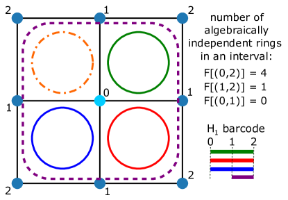
Figure 6: Algebraically independent vs primitive rings. Example of a local atomic environment (LAE) formed by blue atoms, black bonds, and having root atom cyan. The primitive rings [96], are solid green, red, blue and dashed-dotted orange. In contrast, the algebraically independent rings in the LAE are solid green, red, blue, and dashed purple; each of these corresponds to a bar in the $H_{1}$ barcode. The matrix $F[(c,d)]$ (see text) contains information about the the number of algebraically independent rings in the $(c,d)$-shell annulus, $S(c,d)$, of the LAE, where $c$ and $d$ are edge distances of atoms from the root atom, denoted with numbers in the figure. Specifically, the number of algebraically independent rings in the annulus that contains the entire LAE is equal to four ($F[(0,2)]=4$, the four primitive rings). The number of rings in the annulus that excludes the root atom is equal to one (only purple dashed ring, $F[(1,2)]=1$). There are no rings in the annuli containing atoms with edge distance equal to only 0, 1 or 2, or either 0 or 1 ($F[(0,0)]=0$, $F[(1,1)]=0$, $F[(2,2)]=0$, $F[(0,1)]=0$). The $H_{1}$ barcode reproduces the number of algebraically independent rings according to Eq. (19). The dashed-dotted orange ring is not contained in the $H_{1}$ barcode, since it is not algebraically independent from the solid green, red, blue, and dashed purple rings.

Here we summarize the algorithm discussed in Ref. [62] to compute the $H_{1}$ barcode of the atoms-bonds graph obtained from a certain LAE. We denote with $r$ the root atom (center) of the LAE. Given nonnegative integers $c\leq d$, we define the ($c$, $d$)-shell annulus, $S(c,d)$, which is a subgraph of the LAE composed of all atoms (and bonds connecting them) with edge distance (number of bonds on shortest path) between $c$ and $d$ from $r$. To characterize the bond network of the subgraph, it is useful to determine the number of algebraically independent rings in $S(c,d)$, given by:

$$\begin{split}F[(c,d)]=&\;\text{number of components}[S(c,d)]\\ &-\;\text{number of atoms}[S(c,d)]\\ &+\;\text{number of bonds}[S(c,d)].\end{split}$$ (17)

The number of algebraically independent rings is related to the $H_{1}$ barcode as [62]

$$F[(c,d)]={\rm rank}\big{\{}H_{1}[S(c,d)]\big{\}},$$ (18)

i.e., it is the size of the set of rings $H_{1}[S(c,d)]$, that allow to express all other rings by linear combinations. $F[(c,d)]$ can also be resolved in terms of the number of intervals of the form (a, b) (e.g., shown as bars in Fig. 2a) in the $H_{1}$ barcode, denoted with $G[(a,b)]$:

$$F[(c,d)]=\sum_{(a,b)\leq(c,d)}G[(a,b)],$$ (19)

where the sum is taken over annuli ($a$, $b$) contained within or equal to the ($c$, $d$) annulus. As discussed in Ref. [62], the form of Eq. (19) implies that $G[(c,d)]$ can be obtained from $F[(a,b)]$ using Möbius inversion:

$$G[(c,d)]=\sum_{(a,b)\leq(c,d)}F[(a,b)]\mu[(a,b),(c,d)],$$ (20)

where $\mu[(a,b),(c,d)]$ is a Möbius function defined as:

$$\mu[(a,b),(a,b)]=1,$$ (21)

$$\mu[(a,b),(c,d)]=-\sum_{(a,b)\leq(e,f)<(c,d)}\mu[(a,b),(e,f)],$$ (22)

which can be solved recursively. We note that the sum in Eq. (22) is computed over $(a,b)\leq(e,f)<(c,d)$ (excluding the case where $(e,f)=(c,d)$, as implemented in the Swatches software ), correcting a typo present in the original paper [62].

We also note that, in order to characterize and compare disorder across structures with different density, in this work we define LAEs in terms of number of atoms; this differs from the convention adopted by Schweinhart et al. [62], who defined LAEs as a function of number of layers (atoms with the same edge distance to the root). Finally, we note that algebraically independent rings obtained from the intervals $G[(c,d)]$ are not necessarily primitive rings (i.e., rings that cannot be decomposed into smaller rings, see Ref. [96] for details) present in the LAE, see Fig. 6 for an example.

Appendix C BNE and finite-size effects

In Fig. 7 we show the behavior of BNE as a function of LAE’s size $n$ for three models of amorphous carbon that are expected to represent the same physical system, as they have all density $\sim$2.9 g/cm³ and they differ only by simulation-cell size. We see that BNE grows with the LAE’s size $n$, as expected from the extensivity property of the entropy, and then saturates to a constant value ${\rm BNE}_{\rm sat}=\ln{(N_{\rm at})}$ determined by the number of atoms in the simulation cell ($N_{\rm at}$). From a mathematical viewpoint, the saturation occurs when the $H_{1}$ barcode distinguishes all atomic environments, and therefore the distribution of barcodes approaches a uniform distribution with value $1/N_{\rm at}$ for each atom.

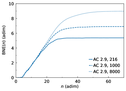
Figure 7: BNE and finite-size effects. Solid, dashed, and dotted lines correspond to 216, 1000, and 8000-atom models of AC with density $\sim$2.9 g/cm³, respectively. $n$ is the number of atoms in the local environments. We note that for $5\lesssim n\lesssim 15$, BNE’s growth rate is approximatively constant and indistinguishable between the three physically equivalent representations of AC considered. We highlight how the finite-size saturation of BNE$(n)$ occurs for larger value of $n$ in larger models. This shows that BNE’s growth rate can be used to characterize structural disorder in AC over lengthscales smaller than the model’s size.

Most importantly, before the finite-size effect saturation occurs, BNE’s growth rate is practically indistinguishable between the three models of AC, suggesting that it can be used to characterize structural disorder in AC over lengthscales smaller than the model’s size. This motivates using BNE’s growth rate as a descriptor for disorder in the bond network of solids.

Appendix D Quasi-degenerate velocity operator

The quasi-degenerate velocity-operator in the frequency representation $\Upsilon(\omega)$ appearing in Eq. (13) is defined as:

$$\begin{split}&\Upsilon^{2}(\omega){=}[\mathcal{G}(\omega)]^{-1}\frac{1}{\mathcal{V}}\sum_{s,s^{\prime}}\frac{\rVert\bm{\mathsfit{v}}_{ss^{\prime}}\lVert^{2}}{3}\delta(\omega{-}\frac{\omega_{s}{+}\omega_{s^{\prime}}}{2})\delta(\omega_{s}{-}\omega_{s^{\prime}}),\end{split}$$ (23)

where $\mathcal{G}(\omega)$ is a density of states defined as

$$\mathcal{G}(\omega)=\frac{1}{N_{at}}\frac{1}{\mathcal{V}}\sum_{s,s^{\prime}}\delta(\omega-\frac{\omega_{s}+\omega_{s^{\prime}}}{2})\delta(\omega_{s}-\omega_{s^{\prime}}).$$ (24)

Appendix E Derivation of the WTE diffusivity in the Explicitly Disordered Glass limit

We start from the first line of Eq. (11) and we use Eq. (23) to approximate the velocity operator elements $\frac{\rVert\bm{\mathsfit{v}}_{ss^{\prime}}\lVert^{2}}{3}$ by a single-frequency dependent function $\frac{\Upsilon^{2}(\omega)}{N_{at}}$,

$$\begin{split}&D_{\rm EDG}(\omega)\!=\!\frac{\pi}{\mathcal{V}g(\omega)}\!\sum_{s,s^{\prime}}\!\frac{\rVert\bm{\mathsfit{v}}_{ss^{\prime}}\lVert^{2}}{3}\!L[\omega_{s}{-}\omega_{s^{\prime}}\!,\Gamma_{s}{+}\Gamma_{s^{\prime}}]\delta(\omega-\omega_{s})\\ &\approx\frac{\pi}{g(\omega)}\frac{\Upsilon^{2}(\omega)}{N_{at}}\left[\frac{1}{\mathcal{V}}\sum_{s,s^{\prime}}\!L[\omega_{s}{-}\omega_{s^{\prime}}\!,\Gamma_{s}{+}\Gamma_{s^{\prime}}]\delta(\omega-\omega_{s})\right].\end{split}$$ (25)

Then, we rewrite the quantity in the square brackets in terms of the convolution:

$$\begin{split}&\left[\frac{1}{\mathcal{V}}\sum_{s,s^{\prime}}\!L[\omega_{s}{-}\omega_{s^{\prime}}\!,\Gamma_{s}{+}\Gamma_{s^{\prime}}]\delta(\omega-\omega_{s})\right]=\\ =&\frac{1}{\mathcal{V}}\sum_{s,s^{\prime}}\!\int\!d(\omega^{\prime}{-}\omega_{s^{\prime}})L[(\omega_{s}{-}\omega_{s^{\prime}})-(\omega^{\prime}{-}\omega_{s^{\prime}})\!,\Gamma_{s}]\\ &\qquad\qquad\times\!L[\omega^{\prime}{-}\omega_{s^{\prime}}\!,\Gamma_{s^{\prime}}]\delta(\omega-\omega_{s})\\ =&\frac{1}{\mathcal{V}}\sum_{s,s^{\prime}}\!\int\!d\omega^{\prime}L[\omega_{s}{-}\omega^{\prime}\!,\Gamma_{s}]L[\omega^{\prime}{-}\omega_{s^{\prime}}\!,\Gamma_{s^{\prime}}]\delta(\omega-\omega_{s})\\ =&\sum_{s}\delta(\omega-\omega_{s})\int\!d\omega^{\prime}L[\omega{-}\omega^{\prime}\!,\Gamma(\omega)]\frac{1}{\mathcal{V}}\sum_{s^{\prime}}\!L[\omega^{\prime}{-}\omega_{s^{\prime}}\!,\Gamma_{s^{\prime}}]\\ =&\mathcal{V}g(\omega)\int\!d\omega^{\prime}L[\omega{-}\omega^{\prime}\!,\Gamma(\omega)]g_{d}(\omega^{\prime})=\mathcal{V}g(\omega)g_{dd}(\omega)\end{split}$$ (26)

where $g_{dd}(\omega)$ denotes the convolution of the dressed VDOS with the Lorentzian with FWHM $\Gamma(\omega)$. In Eq. (LABEL:eq:WDL_derivation2), to go from the first to the second line, we used the property that a Lorentzian with FWHM $\Gamma_{s}{+}\Gamma_{s^{\prime}}$ can be obtained by convolving two Lorentzians with FWHM $\Gamma_{s}$ and $\Gamma_{s^{\prime}}$, respectively. To transform the second line into the third, we changed the variable of integration from $\omega^{\prime}-\omega_{s^{\prime}}$ to $\omega^{\prime}$. From third to fourth line, we exploited the delta function $\delta(\omega-\omega_{s})$ to replace $\omega_{s}$ and $\Gamma_{s}$ in the first Lorentzian to $\omega$ and $\Gamma(\omega)$. $\Gamma(\omega)$ denotes the linewidth evaluated at frequency $\omega$, this notation is possible here because the presence of structural disorder forbids degeneracies and thus allows a bijective mapping between frequency and mode, i.e., $\Gamma_{s}=\Gamma(\omega_{s})=\Gamma(\omega=\omega_{s})$. In the fourth line we also regrouped the terms, and from the fourth to the fifth line we used the definitions of VDOS $\mathcal{V}g(\omega)=\sum_{s}\delta(\omega-\omega_{s})$ and dressed VDOS $g_{d}(\omega^{\prime})$ (Eq. (12)). By combining Eq. (LABEL:eq:WDL_derivation1) and Eq. (LABEL:eq:WDL_derivation2), we obtain the second line of Eq. (11).

If we neglect the influence of the intrinsic linewidth on the broadening of $g_{dd}(\omega)$, then we can approximate the disordered solid to be harmonic, leading to the alternative expression for AF diffusivity shown by Eq. (13). In Fig. 8, we show the numerical equivalence between Eq. (13) and the AF diffusivity in various IRG models.

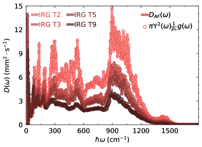
Figure 8: Equivalence between EDG and AF diffusivity in IRG. Solid lines are AF diffusivities in various IRG samples, and the overlapping empty circles are the corresponding WTE diffusivities in the EDG limit (Eq. (13)).

Finally, we discuss how to obtain the self-consistent relation discussed in Eq. (14). We start considering the frequency decomposition equation (Eq. (9)), plug in it the expression (11) for the EDG diffusivity $D(\omega)$, and perform the following algebraic manipulations:

$$\begin{split}\kappa&=\int d\omega\,g(\omega)C(\omega)D(\omega)\\ &=\!\int\!d\omega g(\omega)C(\omega)\pi\Upsilon^{2}(\omega)\frac{1}{\rho_{n}}\!\left[\int\!\!d\omega^{\prime}L[\omega{-}\omega^{\prime}\!,\Gamma(\omega)]g_{d}(\omega^{\prime})\right]\\ &=\pi\frac{1}{\rho_{n}}\iint d\omega d\omega^{\prime}C(\omega)\Upsilon^{2}(\omega)g(\omega)L[\omega{-}\omega^{\prime}\!,\Gamma(\omega)]g_{d}(\omega^{\prime})\\ &\approx\pi\frac{1}{\rho_{n}}\!\int\!d\omega^{\prime}g_{d}(\omega^{\prime})C(\omega^{\prime})\Upsilon^{2}(\omega^{\prime})\!\int\!d\omega g(\omega)L[\omega{-}\omega^{\prime}\!,\Gamma(\omega)]\\ &=\pi\frac{1}{\rho_{n}}\int d\omega^{\prime}g_{d}(\omega^{\prime})C(\omega^{\prime})\Upsilon^{2}(\omega^{\prime})g_{d}(\omega^{\prime})\\ &=\!\!\!\int\!\!\!d\omega g_{d}(\omega)C(\omega)\pi\Upsilon^{2}(\omega)\frac{1}{\rho_{n}}g_{d}(\omega)\!=\!\!\!\int\!\!\!d\omega g_{d}(\omega)C(\omega)D_{d}(\omega),\end{split}$$ (27)

where we denote the dressed diffusivity $D_{d}(\omega)=\pi\Upsilon^{2}(\omega)\frac{1}{\rho_{n}}g_{d}(\omega)$ (i.e., having the same form of Eq. (13), but with bare VDOS replaced by the dressed VDOS). In the third line we reordered the integrals and in the fourth line we used the fact that in derivation of Eq. (11) we used an approximation that the interacting modes have similar frequency due to value of the linewidth $\Gamma(\omega)$ being much smaller than the value of the frequency $\omega$. We used this approximation again here to set $C(\omega)\sim C(\omega^{\prime})$ and $\Upsilon(\omega)\sim\Upsilon(\omega^{\prime})$ for interacting modes. In the fifth line we identify $\int\!d\omega g(\omega)L[\omega{-}\omega^{\prime}\!,\Gamma(\omega)]$ with the dressed VDOS $g_{d}(\omega^{\prime})$. In the sixth line we renamed $\omega^{\prime}$ to $\omega$. The expression in the final line of Eq. (27) is particularly insightful, since the VDOS in the first term and VDOS in the diffusivity are dressed, preserving the property that the diffusivity in disordered systems is proportional to the VDOS. We conclude by noting that the relation between the PDC and EDG conductivities is summarized in Tab. 1.

Table 1: Comparison between the WTE treatments of PDC and EDG.

	Perturbatively Disordered Crystal (PDC)	Explicitly Disordered Glass (EDG)
Transport mechanism	Particle-like propagation	Wave-like tunnelling
VDOS	Not broadened $g(\omega)=g^{\rm DR}_{\rm UOC}(\omega)$	Broadened by structural disorder $g(\omega)=g_{\rm EDG}(\omega)$
Dressed VDOS	Broadened by structural disorder $g_{\rm PDC}(\omega)=\int d\omega^{\prime}L[\omega{-}\omega^{\prime},\Gamma_{\rm dis}(\omega^{\prime})]g^{\rm DR}_{\rm UOC}(\omega^{\prime})$ $g_{d}(\omega)\equiv g_{\rm PDC}(\omega)\approx g_{\rm EDG}(\omega)$	Broadened by disorder and anharmonicity $g_{d}(\omega)=\int d\omega^{\prime}L[\omega{-}\omega^{\prime},\Gamma(\omega^{\prime})]g(\omega^{\prime})$ $g_{d}(\omega)\approx g(\omega)=g_{\rm EDG}(\omega)$
Origin of linewidth	Structural disorder	Intrinsic, e.g. due to isotopes or anharmonicity
Diffusivity	Eq. (10), $D_{\rm PDC}(\omega)=v_{\rm eff}(\omega)\lambda_{\rm eff}(\omega)=\frac{v^{2}_{\rm eff}(\omega)}{\Gamma_{\rm dis}(\omega)}$ and Eq. (14), $D_{\rm PDC}(\omega)=\pi\Upsilon^{2}(\omega)\frac{1}{\rho_{n}}g_{\rm PDC}(\omega)$	Eqs. (11) and (13), $D_{\rm EDG}(\omega){\approx}\pi{\Upsilon^{2}(\omega)}\frac{1}{\rho_{n}}\!\left[\!\int d\omega^{\prime}L[\omega{-}\omega^{\prime}\!,\Gamma(\omega)]g_{d}(\omega^{\prime})\right]$ $\approx\pi{\Upsilon^{2}(\omega)}\frac{1}{\rho_{n}}g_{\rm EDG}(\omega)$
Compatible observables	Thermal conductivity $\kappa$, dressed VDOS $g_{d}(\omega)$, and diffusivity $D(\omega)$

Appendix F Determination of the disorder linewidth from PDC VDOS

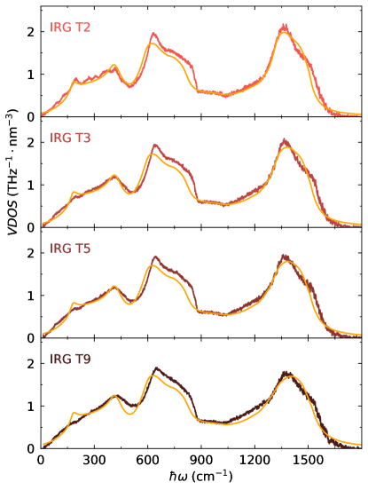
Figure 9: Bare VDOS of IRG vs PDC VDOS. Yellow solid lines are the PDC VDOS obtained dressing the bare VDOS of pristine UOC graphite, and red-to-black lines are bare EDG VDOS of IRG graphite.

In this appendix we discuss the numerical details on how to determine the PDC disorder linewidths $\Gamma(\omega^{\prime})$ that have to be used in Eq. (12) to transform the VDOS of pristine UOC graphite into the VDOS of IRG.

To obtain the density-renormalized VDOS discussed in Sec. VII, $g^{\rm DR}_{\rm UOC}(\omega)$, we proceeded as follows. First, we used the GAP potential [61] to compute second-order interatomic forces in a 8x8x2 supercell, then used these and Fourier-interpolation [98] to compute vibrational frequencies and group velocities on a dense 128x128x32 $\bm{q}$-mesh. By multiplying the frequencies by the factor $a$, as discussed in Sec. VII, we take into account the effect that the density reduction induced by irradiation has on the vibrational frequencies. The bare VDOS was computed using a Lorentzian broadening for the delta functions with FWHM equal to $2\times 0.6$ cm^-1, where 0.6 cm^-1 is the value of the convergence plateau parameter $\eta$ used for thermal conductivity calculations in IRG (see SM for details).

After determining the bare $g^{\rm DR}_{\rm UOC}(\omega)$, we apply to it the dressing transformation 12 to obtain the dressed VDOS of the PDC. When performing such transformation, we assume that the disorder linewidths appearing in the dressing integral assume the established functional form (15); specifically, we calculated the modulus of the group velocity in the frequency representation, $v(\omega)$, which appears in such an expression as:

$$v(\omega)=\frac{\sum_{\bm{q}s}\sqrt{\frac{v^{2}_{\bm{q}s}}{3}}\delta(\omega-a\omega_{\bm{q}s})}{\sum_{\bm{q}s}\delta(\omega-a\omega_{\bm{q}s})},$$ (28)

where sum $\sum_{\bm{q}s}$ runs over the aforementioned 128x128x32 $\bm{q}$-mesh, $\omega_{\bm{q}s}$ is the frequency of the mode $\bm{q}$,$s$ in UOC graphite, and $v_{\bm{q}s}$ the modulus of its group velocity. To evaluate numerically Eq. (28), the Dirac delta distributions are broadened with a Lorentzian having FWHM equal to twice the aforementioned value of the convergence plateau parameter $\eta$ in IRG ($2\times 0.6$ cm^-1). The values for the parameter L and R appearing in Eq. (15) are determined as the values that minimize the Mean Squared Deviation (MSD) between the PDC VDOS and EDG VDOS of irradiated graphite:

$${\rm MSD}=\sum_{i}\left(g_{\rm PDC}(\omega_{i})-g_{\rm EDG}(\omega_{i})\right)^{2}.$$ (29)

This minimization is performed using a stochastic gradient descent optimizer implemented in PyTorch [99].

We show the results of the fits for disorder linewidth $\Gamma_{\rm dis}(\omega)$ in Fig. 5a and the corresponding predictions for the PDC VDOS in Fig. 9. We find that PDC VDOS reasonably replicates the variation with frequency and irradiation dose of the VDOS for all structures of IRG analysed in this work. Finally, we note that after shifting the frequencies of UOC graphite, there are no vibrational modes above ${\sim}1550$ cm^-1. These modes have negligible impact on thermal transport; to decompose IRG’s diffusivity above ${\sim}1550$ cm^-1, we determine the disorder linewidth of frequencies above ${\sim}1550$ cm^-1 as by fitting the linewidth value that matches the tail of disorder linewidth plot in Fig. 5a, finding a linewidth of 24 cm^-1.

Appendix G Influence of anharmonicity on thermal conductivity in IRG

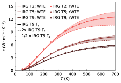
Figure 10: Influence of anharmonicity on thermal conductivity of IRG. Solid, dashed and dotted lines show WTE conductivity calculations for IRG with linewidth equal to linewidth derived from 216-atom model of IRG T9, linewidth of twice this value and linewidth of half this value respectively. The scatter points are rWTE conductivity calculations with linewidth derived from IRG T9 216. Red, brown and black colors denote IRG T2, T5 and T9 respectively.

Fig. 1 shows that the rWTE yields results in agreement with experiments and previous studies based on molecular dynamics. We recall that the rWTE accounts for the influence of anharmonicity only when these are not spuriously affected by finite-size effects. It has been shown in Refs. [60, 67] that the rWTE allows to converge thermal-conductivity calculations faster compared to the bare WTE in ‘strongly disordered’ solids having: (i) disorder-induced repulsion between energy levels [84] comparable to or larger than the intrinsic linewidth ; (ii) average velocity-operator elements nearly constant with respect to the energy difference between two eigenstates [60]. In this ‘strongly disordered’ regime, the rWTE evaluated in a small atomistic model (containing hundreds of atoms) is expected to yield results in agreement with the bare WTE evaluated in a large model (containing several thousands of atoms). In this section we provide additional information to strengthen the claim that in the disordered carbon polymorphs that we studied, structural disorder is the dominant source of thermal resistance and hence the rWTE applied to small models yields results compatible with the WTE applied to very large models. We focus on irradiated graphite, recalling that in Fig. 1 we showed that for IRG T9 the room-temperature rWTE conductivity of a 216-atom model is practically indistinguishable from the bare WTE conductivity of a 14009-atom model. To confirm that disorder is the dominant source of thermal resistance, we evaluate the bare WTE on very large 14009-atom atomistic models and artificially rescale the anharmonic linewidths, enlarging or reducing them by a factor 2. Fig. 10 shows that the lower is structural disorder in IRG, the higher the conductivity and the more relevant are the effects of anharmonicity. Importantly, for all the IRG structures considered, this artificial amplification or reduction of anharmonicity has negligible effect on the conductivity in the temperature range 50< T$\lesssim$ 300K. Since IRG graphite is the class of carbon polymorphs with the largest conductivity and hence most sensitive to anharmonicity, we infer from Fig. 10 that for the polymorphs studied, the conductivity in the temperature range 50< T$\lesssim$ 300K is mainly limited by structural disorder. Our findings are in broad agreement with Refs. [101, 64], which discussed how compositional disorder can yield damping linewidth stronger than those due to anharmonic effects, resulting in a convergent conductivity in the low-temperature limit where anharmonicity phases out.

Finally, we note that upon increasing temperature anharmonicity becomes more relevant—we see that at 700K it is important to use the actual physical values of the anharmonic linewidths. We also highlight how in this high-temperature regime the rWTE and WTE yield indistinguishable results, confirming that anharmonicity is strong enough to dominate over the computational broadening $\eta$ employed in the rWTE (i.e., anharmonic effects are negligibly affected by finite-size effects).

References

- Tian et al. [2023] H. Tian, Y. Ma, Z. Li, M. Cheng, S. Ning, E. Han, M. Xu, P.-F. Zhang, K. Zhao, R. Li, Y. Zou, P. Liao, S. Yu, X. Li, J. Wang, S. Liu, Y. Li, X. Huang, Z. Yao, D. Ding, J. Guo, Y. Huang, J. Lu, Y. Han, Z. Wang, Z. G. Cheng, J. Liu, Z. Xu, K. Liu, P. Gao, Y. Jiang, L. Lin, X. Zhao, L. Wang, X. Bai, W. Fu, J.-Y. Wang, M. Li, T. Lei, Y. Zhang, Y. Hou, J. Pei, S. J. Pennycook, E. Wang, J. Chen, W. Zhou, and L. Liu, Disorder-tuned conductivity in amorphous monolayer carbon, Nature 615, 56 (2023), number: 7950 Publisher: Nature Publishing Group.
- Shang et al. [2021] Y. Shang, Z. Liu, J. Dong, M. Yao, Z. Yang, Q. Li, C. Zhai, F. Shen, X. Hou, L. Wang, N. Zhang, W. Zhang, R. Fu, J. Ji, X. Zhang, H. Lin, Y. Fei, B. Sundqvist, W. Wang, and B. Liu, Ultrahard bulk amorphous carbon from collapsed fullerene, Nature 599, 599 (2021), publisher: Nature Publishing Group.
- Li et al. [2024] Z. Li, A. Bhardwaj, J. He, W. Zhang, T. T. Tran, Y. Li, A. McClung, S. Nuguri, J. J. Watkins, and S.-W. Lee, Nanoporous amorphous carbon nanopillars with lightweight, ultrahigh strength, large fracture strain, and high damping capability, Nature Communications 15, 8151 (2024), publisher: Nature Publishing Group.
- Statz et al. [2020] M. Statz, S. Schneider, F. J. Berger, L. Lai, W. A. Wood, M. Abdi-Jalebi, S. Leingang, H.-J. Himmel, J. Zaumseil, and H. Sirringhaus, Charge and Thermoelectric Transport in Polymer-Sorted Semiconducting Single-Walled Carbon Nanotube Networks, ACS Nano 14, 15552 (2020), publisher: American Chemical Society.
- Liu et al. [2024] X. Liu, D. Lyu, C. Merlet, M. J. A. Leesmith, X. Hua, Z. Xu, C. P. Grey, and A. C. Forse, Structural disorder determines capacitance in nanoporous carbons, Science 384, 321 (2024), publisher: American Association for the Advancement of Science.
- Simoncelli et al. [2018] M. Simoncelli, N. Ganfoud, A. Sene, M. Haefele, B. Daffos, P.-L. Taberna, M. Salanne, P. Simon, and B. Rotenberg, Blue Energy and Desalination with Nanoporous Carbon Electrodes: Capacitance from Molecular Simulations to Continuous Models, Physical Review X 8, 021024 (2018), publisher: American Physical Society.
- Jeanmairet et al. [2022] G. Jeanmairet, B. Rotenberg, and M. Salanne, Microscopic Simulations of Electrochemical Double-Layer Capacitors, Chemical Reviews 122, 10860 (2022), publisher: American Chemical Society.
- Liu et al. [2017] D. Liu, B. Gludovatz, H. S. Barnard, M. Kuball, and R. O. Ritchie, Damage tolerance of nuclear graphite at elevated temperatures, Nature Communications 8, 15942 (2017), publisher: Nature Publishing Group.
- Farbos et al. [2017] B. Farbos, H. Freeman, T. Hardcastle, J.-P. Da Costa, R. Brydson, A. J. Scott, P. Weisbecker, C. Germain, G. L. Vignoles, and J.-M. Leyssale, A time-dependent atomistic reconstruction of severe irradiation damage and associated property changes in nuclear graphite, Carbon 120, 111 (2017).
- Prasher et al. [2009] R. S. Prasher, X. J. Hu, Y. Chalopin, N. Mingo, K. Lofgreen, S. Volz, F. Cleri, and P. Keblinski, Turning Carbon Nanotubes from Exceptional Heat Conductors into Insulators, Physical Review Letters 102, 105901 (2009), publisher: American Physical Society.
- Mehew et al. [2023] J. D. Mehew, M. Y. Timmermans, D. Saleta Reig, S. Sergeant, M. Sledzinska, E. Chávez-Ángel, E. Gallagher, C. M. Sotomayor Torres, C. Huyghebaert, and K.-J. Tielrooij, Enhanced Thermal Conductivity of Free-Standing Double-Walled Carbon Nanotube Networks, ACS Applied Materials & Interfaces 15, 51876 (2023), publisher: American Chemical Society.
- Kern et al. [2016] A. M. Kern, B. Zierath, J. Haertlé, T. Fey, and B. J. M. Etzold, Thermal and Electrical Conductivity of Amorphous and Graphitized Carbide-Derived Carbon Monoliths, Chemical Engineering & Technology 39, 1121 (2016).
- Pop et al. [2012] E. Pop, V. Varshney, and A. K. Roy, Thermal properties of graphene: Fundamentals and applications, MRS Bulletin 37, 1273 (2012).
- Lee et al. [2015] S. Lee, D. Broido, K. Esfarjani, and G. Chen, Hydrodynamic phonon transport in suspended graphene, Nat. Commun. 6, 6290 (2015).
- Pereira and Donadio [2013] L. F. C. Pereira and D. Donadio, Divergence of the thermal conductivity in uniaxially strained graphene, Physical Review B 87, 125424 (2013), publisher: American Physical Society.
- Barbarino et al. [2015] G. Barbarino, C. Melis, and L. Colombo, Intrinsic thermal conductivity in monolayer graphene is ultimately upper limited: A direct estimation by atomistic simulations, Physical Review B 91, 035416 (2015), publisher: American Physical Society.
- Majee and Aksamija [2018] A. K. Majee and Z. Aksamija, Dynamical thermal conductivity of suspended graphene ribbons in the hydrodynamic regime, Phys. Rev. B 98, 024303 (2018).
- Braun et al. [2022] O. Braun, R. Furrer, P. Butti, K. Thodkar, I. Shorubalko, I. Zardo, M. Calame, and M. L. Perrin, Spatially mapping thermal transport in graphene by an opto-thermal method, NPJ 2D Mater. Appl. 6, 1 (2022).
- Han and Ruan [2023] Z. Han and X. Ruan, Thermal conductivity of monolayer graphene: Convergent and lower than diamond, Physical Review B 108, L121412 (2023), publisher: American Physical Society.
- Fugallo et al. [2014] G. Fugallo, A. Cepellotti, L. Paulatto, M. Lazzeri, N. Marzari, and F. Mauri, Thermal Conductivity of Graphene and Graphite: Collective Excitations and Mean Free Paths, Nano Lett. 14, 6109 (2014).
- Zhang et al. [2016] H. Zhang, X. Chen, Y.-D. Jho, and A. J. Minnich, Temperature-Dependent Mean Free Path Spectra of Thermal Phonons Along the c-Axis of Graphite, Nano Letters 16, 1643 (2016), publisher: American Chemical Society.
- Huberman et al. [2019] S. Huberman, R. A. Duncan, K. Chen, B. Song, V. Chiloyan, Z. Ding, A. A. Maznev, G. Chen, and K. A. Nelson, Observation of second sound in graphite at temperatures above 100 K, Science 364, 375 (2019).
- Machida et al. [2020] Y. Machida, N. Matsumoto, T. Isono, and K. Behnia, Phonon hydrodynamics and ultrahigh–room-temperature thermal conductivity in thin graphite, Science 367, 309 (2020).
- Jeong et al. [2021] J. Jeong, X. Li, S. Lee, L. Shi, and Y. Wang, Transient hydrodynamic lattice cooling by picosecond laser irradiation of graphite, Phys. Rev. Lett. 127, 085901 (2021).
- Ding et al. [2022] Z. Ding, K. Chen, B. Song, J. Shin, A. A. Maznev, K. A. Nelson, and G. Chen, Observation of second sound in graphite over 200 K, Nature Communications 13, 285 (2022).
- Huang et al. [2023] X. Huang, Y. Guo, Y. Wu, S. Masubuchi, K. Watanabe, T. Taniguchi, Z. Zhang, S. Volz, T. Machida, and M. Nomura, Observation of phonon Poiseuille flow in isotopically purified graphite ribbons, Nat. Commun. 14, 2044 (2023).
- Huang et al. [2024] X. Huang, R. Anufriev, L. Jalabert, K. Watanabe, T. Taniguchi, Y. Guo, Y. Ni, S. Volz, and M. Nomura, A graphite thermal Tesla valve driven by hydrodynamic phonon transport, Nature , 1 (2024), publisher: Nature Publishing Group.
- Dragašević and Simoncelli [2024] J. Dragašević and M. Simoncelli, Viscous heat backflow and temperature resonances in extreme thermal conductors (2024), arXiv:2303.12777 [cond-mat].
- Balandin [2011] A. A. Balandin, Thermal properties of graphene and nanostructured carbon materials, Nature Materials 10, 569 (2011), number: 8 Publisher: Nature Publishing Group.
- Goblot et al. [2024] V. Goblot, K. Wu, E. D. Lucente, Y. Zhu, E. Losero, Q. Jobert, C. J. Concha, N. Marzari, M. Simoncelli, and C. Galland, Imaging heat transport in suspended diamond nanostructures with integrated spin defect thermometers (2024), arXiv:2411.04065.
- Morath et al. [1994] C. J. Morath, H. J. Maris, J. J. Cuomo, D. L. Pappas, A. Grill, V. V. Patel, J. P. Doyle, and K. L. Saenger, Picosecond optical studies of amorphous diamond and diamondlike carbon: Thermal conductivity and longitudinal sound velocity, Journal of Applied Physics 76, 2636 (1994).
- Hurler et al. [1995] W. Hurler, M. Pietralla, and A. Hammerschmidt, Determination of thermal properties of hydrogenated amorphous carbon films via mirage effect measurements, Diamond and Related Materials 4, 954 (1995).
- Bullen et al. [2000] A. J. Bullen, K. E. O’Hara, D. G. Cahill, O. Monteiro, and A. von Keudell, Thermal conductivity of amorphous carbon thin films, Journal of Applied Physics 88, 6317 (2000).
- Shamsa et al. [2006] M. Shamsa, W. L. Liu, A. A. Balandin, C. Casiraghi, W. I. Milne, and A. C. Ferrari, Thermal conductivity of diamond-like carbon films, Applied Physics Letters 89, 161921 (2006).
- Scott et al. [2021] E. A. Scott, S. W. King, N. N. Jarenwattananon, W. A. Lanford, H. Li, J. Rhodes, and P. E. Hopkins, Thermal Conductivity Enhancement in Ion-Irradiated Hydrogenated Amorphous Carbon Films, Nano Letters 21, 3935 (2021), publisher: American Chemical Society.
- Arlein et al. [2008] J. L. Arlein, S. E. M. Palaich, B. C. Daly, P. Subramonium, and G. A. Antonelli, Optical pump-probe measurements of sound velocity and thermal conductivity of hydrogenated amorphous carbon films, Journal of Applied Physics 104, 033508 (2008).
- Chen et al. [2000] G. Chen, P. Hui, and S. Xu, Thermal conduction in metalized tetrahedral amorphous carbon (ta–C) films on silicon, Thin Solid Films 366, 95 (2000).
- Maruyama and Harayama [1992] T. Maruyama and M. Harayama, Neutron irradiation effect on the thermal conductivity and dimensional change of graphite materials, Journal of Nuclear Materials 195, 44 (1992).
- Wu et al. [1994] C. H. Wu, J. P. Bonal, B. Thiele, G. Tsotridis, H. Kwast, H. Werle, J. P. Coad, G. Federici, and G. Vieider, Neutron irradiation effects on the properties of carbon materials, Journal of Nuclear Materials 212-215, 416 (1994).
- Snead and Burchell [1995a] L. Snead and T. Burchell, Reduction in thermal conductivity due to neutron irradiation, 22nd Biennial Conference on Carbon (1995a).
- Snead and Burchell [1995b] L. L. Snead and T. D. Burchell, Thermal conductivity degradation of graphites due to nuetron irradiation at low temperature, Journal of Nuclear Materials 224, 222 (1995b).
- Bonal and Wu [1996] J. Bonal and C. Wu, Neutron irradiation effects on the thermal conductivity and dimensional stability of carbon fiber composites at divertor conditions, Journal of Nuclear Materials 228, 155 (1996).
- Ishiyama et al. [1996] S. Ishiyama, T. Burchell, J. Strizak, and M. Eto, The effect of high fluence neutron irradiation on the properties of a fine-grained isotropic nuclear graphite, Journal of Nuclear Materials 230, 1 (1996).
- Barabash et al. [2002] V. Barabash, I. Mazul, R. Latypov, A. Pokrovsky, and C. Wu, The effect of low temperature neutron irradiation and annealing on the thermal conductivity of advanced carbon-based materials, Journal of Nuclear Materials 307-311, 1300 (2002).
- Snead [2008] L. L. Snead, Accumulation of thermal resistance in neutron irradiated graphite materials, Journal of Nuclear Materials Proceedings of the Seventh and Eighth International Graphite Specialists Meetings (INGSM), 381, 76 (2008).
- Campbell et al. [2016] A. A. Campbell, Y. Katoh, M. A. Snead, and K. Takizawa, Property changes of G347A graphite due to neutron irradiation, Carbon 109, 860 (2016).
- Heijna et al. [2017] M. Heijna, S. De Groot, and J. Vreeling, Comparison of irradiation behaviour of HTR graphite grades, Journal of Nuclear Materials 492, 148 (2017).
- Maruyama and Li [2019] T. Maruyama and Z. Li, Dimensional changes and thermal conductivity by annealing and its relation to the defect concentration and stored energy release of neutron-irradiated graphite, Journal of Nuclear Science and Technology 56, 1006 (2019), publisher: Taylor & Francis _eprint: https://doi.org/10.1080/00223131.2019.1633966.
- Zhou et al. [2024] X. Zhou, Y. Liu, B. Tang, J. Wang, H. Dong, X. Xiu, S. Chen, and Z. Fan, Million-atom heat transport simulations of polycrystalline graphene approaching first-principles accuracy enabled by neuroevolution potential on desktop GPUs (2024), arXiv:2410.13535 [cond-mat].
- Giri et al. [2022] A. Giri, C. J. Dionne, and P. E. Hopkins, Atomic coordination dictates vibrational characteristics and thermal conductivity in amorphous carbon, npj Computational Materials 8, 1 (2022), number: 1 Publisher: Nature Publishing Group.
- Minamitani et al. [2022] E. Minamitani, T. Shiga, M. Kashiwagi, and I. Obayashi, Relationship between local coordinates and thermal conductivity in amorphous carbon, Journal of Vacuum Science & Technology A 40, 033408 (2022).
- Moon and Tian [2024] J. Moon and Z. Tian, Crystal-like thermal transport in amorphous carbon (2024), arXiv:2405.07298 [cond-mat].
- Lv and Henry [2016a] W. Lv and A. Henry, Phonon transport in amorphous carbon using Green–Kubo modal analysis, Applied Physics Letters 108, 181905 (2016a).
- Suarez-Martinez and Marks [2011] I. Suarez-Martinez and N. A. Marks, Effect of microstructure on the thermal conductivity of disordered carbon, Applied Physics Letters 99, 033101 (2011).
- Zhang et al. [2017] X.-X. Zhang, L.-Q. Ai, M. Chen, and D.-X. Xiong, Thermal conductive performance of deposited amorphous carbon materials by molecular dynamics simulation, Molecular Physics 115, 831 (2017), publisher: Taylor & Francis _eprint: https://doi.org/10.1080/00268976.2017.1288940.
- Wang et al. [2024] Y. Wang, Z. Fan, P. Qian, M. A. Caro, and T. Ala-Nissila, Density dependence of thermal conductivity in nanoporous and amorphous carbon with machine-learned molecular dynamics (2024), arXiv:2408.12390 [cond-mat].
- Jung et al. [2017] G. S. Jung, J. Yeo, Z. Tian, Z. Qin, and M. J. Buehler, Unusually low and density-insensitive thermal conductivity of three-dimensional gyroid graphene, Nanoscale 9, 13477 (2017), publisher: The Royal Society of Chemistry.
- Simoncelli et al. [2019] M. Simoncelli, N. Marzari, and F. Mauri, Unified theory of thermal transport in crystals and glasses, Nature Physics 15, 809 (2019).
- Simoncelli et al. [2022] M. Simoncelli, N. Marzari, and F. Mauri, Wigner Formulation of Thermal Transport in Solids, Physical Review X 12, 041011 (2022).
- Simoncelli et al. [2023] M. Simoncelli, F. Mauri, and N. Marzari, Thermal conductivity of glasses: first-principles theory and applications, npj Computational Materials 9, 1 (2023), number: 1 Publisher: Nature Publishing Group.
- Rowe et al. [2020] P. Rowe, V. L. Deringer, P. Gasparotto, G. Csányi, and A. Michaelides, An accurate and transferable machine learning potential for carbon, The Journal of Chemical Physics 153, 034702 (2020).
- Schweinhart et al. [2020] B. Schweinhart, D. Rodney, and J. K. Mason, Statistical topology of bond networks with applications to silica, Physical Review E 101, 052312 (2020).
- Fiorentino et al. [2023] A. Fiorentino, P. Pegolo, and S. Baroni, Hydrodynamic finite-size scaling of the thermal conductivity in glasses, npj Computational Materials 9, 1 (2023), publisher: Nature Publishing Group.
- Fiorentino et al. [2024a] A. Fiorentino, P. Pegolo, S. Baroni, and D. Donadio, Effects of colored disorder on the heat conductivity of SiGe alloys from first principles (2024a), arXiv:2408.05155 [cond-mat].
- Zhang et al. [2022] Z. Zhang, Y. Guo, M. Bescond, J. Chen, M. Nomura, and S. Volz, How coherence is governing diffuson heat transfer in amorphous solids, npj Computational Materials 8, 96 (2022).
- Simoncelli et al. [2024] M. Simoncelli, D. Fournier, M. Marangolo, E. Balan, K. Béneut, B. Baptiste, B. Doisneau, N. Marzari, and F. Mauri, Temperature-invariant heat conductivity from compensating crystalline and glassy transport: from the Steinbach meteorite to furnace bricks (2024), arXiv:2405.13161 [cond-mat].
- Harper et al. [2024] A. F. Harper, K. Iwanowski, W. C. Witt, M. C. Payne, and M. Simoncelli, Vibrational and thermal properties of amorphous alumina from first principles, Physical Review Materials 8, 043601 (2024), publisher: American Physical Society.
- Allen and Feldman [1989] P. B. Allen and J. L. Feldman, Thermal Conductivity of Glasses: Theory and Application to Amorphous Si, Physical Review Letters 62, 645 (1989).
- Palmer et al. [2010] J. C. Palmer, A. Llobet, S. H. Yeon, J. E. Fischer, Y. Shi, Y. Gogotsi, and K. E. Gubbins, Modeling the structural evolution of carbide-derived carbons using quenched molecular dynamics, Carbon 48, 1116 (2010).
- Deringer et al. [2018] V. L. Deringer, C. Merlet, Y. Hu, T. H. Lee, J. A. Kattirtzi, O. Pecher, G. Csányi, S. R. Elliott, and C. P. Grey, Towards an atomistic understanding of disordered carbon electrode materials, Chemical Communications 54, 5988 (2018), publisher: The Royal Society of Chemistry.
- de Tomas et al. [2019] C. de Tomas, A. Aghajamali, J. L. Jones, D. J. Lim, M. J. López, I. Suarez-Martinez, and N. A. Marks, Transferability in interatomic potentials for carbon, Carbon 155, 624 (2019).
- Allen et al. [1999] P. B. Allen, J. L. Feldman, J. Fabian, and F. Wooten, Diffusons, Locons, Propagons: Character of Atomic Vibrations in Amorphous Si, Philosophical Magazine B 79, 1715 (1999), arXiv:cond-mat/9907132.
- Fiorentino et al. [2024b] A. Fiorentino, E. Drigo, S. Baroni, and P. Pegolo, Unearthing the foundational role of anharmonicity in heat transport in glasses, Physical Review B 109, 224202 (2024b).
- Puligheddu et al. [2019] M. Puligheddu, Y. Xia, M. Chan, and G. Galli, Computational prediction of lattice thermal conductivity: A comparison of molecular dynamics and Boltzmann transport approaches, Physical Review Materials 3, 085401 (2019).
- Elliott [1991] S. R. Elliott, Medium-range structural order in covalent amorphous solids, Nature 354, 445 (1991).
- Milkus et al. [2018] R. Milkus, C. Ness, V. V. Palyulin, J. Weber, A. Lapkin, and A. Zaccone, Interpretation of the Vibrational Spectra of Glassy Polymers Using Coarse-Grained Simulations, Macromolecules 51, 1559 (2018), publisher: American Chemical Society.
- Wallace [1972] D. C. Wallace, Thermodynamics of Crystals (1972).
- Kittel [1949] C. Kittel, Interpretation of the Thermal Conductivity of Glasses, Physical Review 75, 972 (1949), publisher: American Physical Society.
- Casimir [1938] H. B. G. Casimir, Note on the conduction of heat in crystals, Physica 5, 495 (1938).
- Peierls [2001] R. E. Peierls, Quantum theory of solids (Oxford Classics Series, 2001).
- MARADUDIN and VOSKO [1968] A. A. MARADUDIN and S. H. VOSKO, Symmetry Properties of the Normal Vibrations of a Crystal, Reviews of Modern Physics 40, 1 (1968), publisher: American Physical Society.
- Prat et al. [2016] T. Prat, N. Cherroret, and D. Delande, Semiclassical spectral function and density of states in speckle potentials, Physical Review A 94, 022114 (2016), publisher: American Physical Society.
- Chandrasekaran and Betouras [2022] A. Chandrasekaran and J. J. Betouras, Effect of disorder on density of states and conductivity in higher-order Van Hove singularities in two-dimensional bands, Physical Review B 105, 075144 (2022), publisher: American Physical Society.
- Simkin and Mahan [2000] M. V. Simkin and G. D. Mahan, Minimum Thermal Conductivity of Superlattices, Physical Review Letters 84, 927 (2000).
- Ziman [1960] Ziman, Electrons and Phonons: The Theory of Transport in solids (1960).
- Hanus et al. [2021] R. Hanus, R. Gurunathan, L. Lindsay, M. T. Agne, J. Shi, S. Graham, and G. Jeffrey Snyder, Thermal transport in defective and disordered materials, Applied Physics Reviews 8, 031311 (2021).
- Osipov and Krasavin [1998] V. A. Osipov and S. E. Krasavin, Disclination dipoles as the basic structural elements of dielectric glasses, Physics Letters A 250, 369 (1998).
- Karthik et al. [2011] C. Karthik, J. Kane, D. P. Butt, W. E. Windes, and R. Ubic, In situ transmission electron microscopy of electron-beam induced damage process in nuclear grade graphite, Journal of Nuclear Materials 412, 321 (2011).
- Tamura [1983] S.-i. Tamura, Isotope scattering of dispersive phonons in Ge, Physical Review B 27, 858 (1983), publisher: American Physical Society.
- Note [1] Specifically, the form of the factor derives from: (i) considering an elementary Debye model having speed of sound and Debye frequency ; (ii) assuming the main change in the frequencies when lowering the density of graphite is mainly due to changes in the volume and has negligible effect on . This implies that the frequencies scale with the cube root of the density: .
- Conyuh and Beltukov [2021] D. A. Conyuh and Y. M. Beltukov, Random matrix approach to the boson peak and Ioffe-Regel criterion in amorphous solids, Physical Review B 103, 104204 (2021).
- Ciarella et al. [2023] S. Ciarella, D. Khomenko, L. Berthier, F. C. Mocanu, D. R. Reichman, C. Scalliet, and F. Zamponi, Finding defects in glasses through machine learning, Nature Communications 14, 4229 (2023), publisher: Nature Publishing Group.
- Luo et al. [2020] Y. Luo, X. Yang, T. Feng, J. Wang, and X. Ruan, Vibrational hierarchy leads to dual-phonon transport in low thermal conductivity crystals, Nature Communications 11, 2554 (2020).
- Legenstein et al. [2024] L. Legenstein, L. Reicht, S. Wieser, M. Simoncelli, and E. Zojer, Heat transport in crystalline organic semiconductors: coexistence of phonon propagation and tunneling (2024), arXiv:2412.05062 [cond-mat].
- Lv and Henry [2016b] W. Lv and A. Henry, Non-negligible Contributions to Thermal Conductivity From Localized Modes in Amorphous Silicon Dioxide, Scientific Reports 6, 35720 (2016b).
- Le Roux and Jund [2010] S. Le Roux and P. Jund, Ring statistics analysis of topological networks: New approach and application to amorphous GeS2 and SiO2 systems, Computational Materials Science 49, 70 (2010).
- Note [2] https://github.com/bschweinhart/Swatches.
- Togo [2023] A. Togo, First-principles Phonon Calculations with Phonopy and Phono3py, Journal of the Physical Society of Japan 92, 012001 (2023).
- Paszke et al. [2019] A. Paszke, S. Gross, F. Massa, A. Lerer, J. Bradbury, G. Chanan, T. Killeen, Z. Lin, N. Gimelshein, L. Antiga, A. Desmaison, A. Kopf, E. Yang, Z. DeVito, M. Raison, A. Tejani, S. Chilamkurthy, B. Steiner, L. Fang, J. Bai, and S. Chintala, Pytorch: An imperative style, high-performance deep learning library, in Advances in Neural Information Processing Systems 32 (Curran Associates, Inc., 2019) pp. 8024–8035.
- Note [3] We recall that stronger disorder-induced repulsion between energy levels promotes a smoother VDOS.
- Thébaud et al. [2023] S. Thébaud, L. Lindsay, and T. Berlijn, Breaking Rayleigh’s Law with Spatially Correlated Disorder to Control Phonon Transport, Physical Review Letters 131, 026301 (2023), publisher: American Physical Society.