Revealing spinons by proximity effect

Abstract

The ghost-Gutzwiller variational wavefunction within the Gutzwiller approximation is shown to stabilise a genuine paramagnetic Mott insulator in the half-filled single-band Hubbard model. This phase hosts quasiparticles that are crucial to the paramagnetic response without showing up in the single-particle spectrum, and, as such, they can be legitimately regarded as an example of Anderson’s spinons. We demonstrate that these spinons at the interface with a metal reacquire charge by proximity effect and thus reemerge in the spectrum as a heavy-fermion band.

Introduction

Quantum spin liquids are Mott insulators that host local moments which do not order down to very low temperatures and yet exhibit mutual long-range quantum entanglement well above those temperatures [1, 2]. The elementary excitations of such systems at energies below the Mott-Hubbard single-particle gap cannot carry electric charge, but they may carry spin as well as possibly emergent quantum numbers [1, 2, 3, 4, 5]. A celebrated example of these excitations are Anderson’s spinons [6, 7], which arise in the uniform resonating valence bond states proposed to describe highly frustrated spin-1/2 Heisenberg models and weakly-doped Mott insulators [6, 7, 8, 9]. These are neutral gapless spin-1/2 quasiparticles that possess a well-defined Fermi surface. Even though such Fermi surface is likely to suffer from a low-temperature instability opening a finite spin-gap $\Delta_{sp}$ [10, 11, 12, 13, 14], one could envisage the possibility of a spinon degeneracy temperature $T_{sp}$ much larger than $\Delta_{sp}$, which would imply that gapless spinons still characterize the physical behaviour for temperatures $\Delta_{sp}\ll T\ll T_{sp}$, or, possibly, at finite magnetic fields [15]. In those circumstances, a spinon Fermi surface would reveal itself in inelastic neutron scattering [16, 17] or thermal properties [18, 19, 20, 21, 22, 23]. Alternatively, spinons can be detected by more local probes, e.g., through their ability to Kondo screen magnetic impurities [24, 25, 26], or by making proper interfaces with the quantum spin-liquid [27, 28, 29, 30, 31].

In this work we show that even the simplest interface with a conventional metal might be suitable to reveal the spinons hosted in a quantum spin-liquid Mott insulator. Hereafter, we assume a simplified portrait of a quantum spin-liquid, specifically, the paramagnetic Mott insulator that can be stabilized in the single-band Hubbard model forcing spin-$SU(2)$ symmetry within the so-called ghost-Gutzwiller approximation [32]. Such interface has already been studied at particle-hole symmetry by Helmes, Costi and Rosch [33] using dynamical mean-field theory (DMFT) [34]. They showed that the metal penetrates inside the Mott insulator creating a narrow quasiparticle peak that decays exponentially inside the insulating slab over a length that corresponds to the correlation length associated to the Mott transition. This result, later reproduced in [35] using the standard Gutzwiller approximation, was interpreted as a Kondo-like proximity effect: the Mott insulator hosts localized moments which are promoted into genuine Kondo resonances by the coupling with the metal [33]. While it seems tempting to identify those local moments with spinons a priori, such interpretation does not stand up to detailed scrutiny. Indeed, the paramagnetic Mott insulator that is stabilized in DMFT has an extensive spin entropy, $\ln 2$ per site [34], as if the local moments were completely free, thus lacking the massive entanglement characterizing quantum spin liquids. Exactly the same occurs in the standard Gutzwiller approximation [36], where the Mott insulator is a trivial state of independent sites, each occupied by a single electron. At the meantime, the DMFT Mott insulator is claimed to exhibit a finite uniform paramagnetic spin susceptibility [34], which seems not truly consistent with its extensive entropy, nor with the evidence that a straight $T=0$ DMFT calculation in the Mott insulator at weak magnetic fields does not converge [37], barring access to the magnetic susceptibility calculated through the magnetization versus field. The reason of this inconsistency seems to lie in the iterative method through which the DMFT self-consistency equation is solved [38]. Indeed, to reach convergence in the Mott insulator within the usual iterative scheme, one is forced to assume that the Anderson impurity model onto which the lattice model maps is not described by a pure state, as is expected at $T=0$, but by a mixed one, sum of two states with opposite spin polarizations.
To address this shortcoming, we decided to use the ghost-Gutzwiller approximation [32], which is rigorously variational in the limit of infinite lattice-coordination, and which is able to stabilize a genuine, zero-entropy, paramagnetic Mott insulator [38]. This hints at the existence of spinons, whose presence we aim to trace out. In particular, and to better highlight the chargeless nature of spinons, in this work we investigate a metal-Mott insulator interface away from the particle-hole (p-h) symmetric value of the chemical potential. For completeness, we start with the standard Gutzwiller approximation (Gut) [39, 40, 41, 42, 43, 44], since the Mott transition changes nature away from p-h symmetry and becomes first order. This change of character has been exploited in [45] to study by DMFT the interface between metal and Mott insulator phases coexisting at equilibrium. We next move to the main part of our work, namely, the interface studied by the ghost-Gutzwiller approximation (gGut) [32, 38, 46, 47, 48, 49, 50, 51, 52, 53]. Specifically, the paper is organised as follows: in section I we give a brief introduction to the Gutzwiller and ghost-Gutzwiller approximations for the Metal-Mott interface. In section II, we present results using the standard Gut and show how the phenomenology of the Kondo proximity effect extends to non particle-hole symmetric cases. In section III we study the same model by the gGut. Finally, in section IV, we discuss the results by solving analytically the gGut variational problem for a bulk Mott insulator in the limit of a very large Mott-Hubbard gap. In that limit, we also show the solution forcing a finite spin-polarization, which clearly unveils the role of spinon in allowing the Mott insulator to sustain partial spin-polarization, and gives access to the paramagnetic susceptibility. Section V is devoted to conclusions.

I Model and methods

In Fig. 1 we show the system under investigation, which consists of a set of metallic layers, represented as weakly interacting Hubbard models, coupled to several Mott insulating ones, strongly interacting Hubbard models. The system has a total of $N$ layers and the interlayer coupling is just a single particle hopping. We assume that intralayer and interlayer hopping strengths are equal, while the difference between metallic and Mott-insulating layers is modelled by a layer-dependent Hubbard repulsion. The system is therefore described by the Hamiltonian:

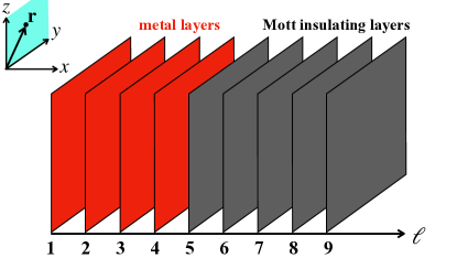
Figure 1: Schematic representation of the slab geometry in the case of 9 layers, 4 of which are metallic, in red, and the rest Mott insulating, in grey. Layers are stacked along the $x$-axis, while a site in each layer is identified by the vector $\mathbf{r}$ in the $y$-$z$ plane.

$$\mathcal{H} =\sum_{\ell=1}^{N}\,\sum_{\mathbf{k}\sigma}\,\epsilon_{\mathbf{k}}\,c^{\dagger}_{\ell\mathbf{k}\sigma}\,c^{\phantom{\dagger}}_{\ell\mathbf{k}\sigma}$$ (1)

$$\quad-t\,\sum_{\ell=1}^{N-1}\,\sum_{\mathbf{k}\sigma}\,\big{(}c^{\dagger}_{\ell+1\mathbf{k}\sigma}\,c^{\phantom{\dagger}}_{\ell\mathbf{k}\sigma}+H.c.\big{)}$$

$$\qquad+\sum_{\ell=1}^{N}\,\sum_{\mathbf{r}}\bigg{\{}\frac{U_{\ell}}{2}\,\big{(}n_{\ell\mathbf{r}}-1\big{)}^{2}-\delta\mu\,n_{\ell\mathbf{r}}\bigg{\}}\,,$$

where the lattice sites are identified by an intralayer coordinate $\mathbf{r}$ and a layer index $\ell=1,\dots,N$, and thus $n_{\ell\mathbf{r}}$ is the on-site occupation number, while the non-interacting intra-layer dispersion $\epsilon_{\mathbf{k}}=-2t\,(\cos k_{y}+\cos k_{z})$, with $\mathbf{k}$ the momentum in the $y$-$z$ plane. Hereafter, we take $t=1$ as energy unit. We remark that $\delta\mu$ in Eq. (1) parametrizes the deviation with respect to the p-h symmetric case, $\delta\mu=0$, while the physical chemical potential is in reality $\mu=U/2+\delta\mu$.
As mentioned in the introduction, we study the system by means of the Gutzwiller (both standard and ghost) approximation [35, 32]. The Gutzwiller variational wavefunction $\ket{\Psi}$ consists of an uncorrelated variational Slater determinant $\ket{\Psi_{*}}$, defined in a (possibly enlarged) auxiliary Hilbert space, which is projected by a linear operator $\mathcal{P}_{G}$ onto the physical Hilbert space. The conventional Gutzwiller wavefunction [39, 40] corresponds to the case in which the dimensions of the physical and auxiliary Hilbert spaces coincide, while, if the auxiliary Hilbert space is larger than the physical one, we talk about the ghost-Gutzwiller wavefunction [32]. The inclusion of additional auxiliary fermions extends the variational freedom and gives access to high-energy spectral features such as the Hubbard bands [32].
For the case of the Hamiltonian in Eq. (1) the variational wavefunction reads:

$$\ket{\Psi} =\mathcal{P}_{G}\ket{\Psi_{*}}\,,$$ (2)

$$\mathcal{P}_{G} =\prod_{\mathbf{r},\ell}\Bigg{\{}\sum_{\gamma,\Gamma}\,\lambda_{\gamma,\Gamma}(\ell)\ket{\mathbf{r},\ell;\gamma}\bra{\mathbf{r},\ell;\Gamma}\Bigg{\}}\,.$$

The states $\Gamma$ are local Fock states of the auxiliary fermions, whose annihilation operators we denote as $d^{\phantom{\dagger}}_{\ell\mathbf{r}\alpha\sigma}$, where $\alpha=1,\dots,N_{aux}$ span the auxiliary spinful orbitals. On the contrary, the set $\gamma$ includes the local physical Fock states.
In Eq. (2) we have assumed translational invariance within each layer, so that our variational parameters depend only on the $\ell$ coordinate. This also implies that the variational wavefunction Eq. (2) cannot develop the antiferromagnetic order parameter that characterizes the actual ground state of Eq. (1) at finite on-site repulsion. Such restriction into a subspace of the whole Hilbert space, which does not include the expected ground state in the specific example, is easy to implement in the variational approach.
Following [43], we can associate the parameters $\lambda_{\gamma,\Gamma}(\mathbf{r},\ell)$ to the components of a wavefunction that describes an impurity coupled to $N_{aux}$ baths. In the slab geometry, we need an impurity wavefunction $\ket{\phi(\ell)}$ for each layer. Using the Gutzwiller approximation, specified in Appendix A, we can write the variational energy as:

$$E[\Psi]=\bra{\Psi_{*}}\mathcal{H}_{*}\ket{\Psi_{*}}+\mathcal{A}\sum_{\ell}\,\bra{\phi(\ell)}\mathcal{H}_{loc}(\ell)\ket{\phi(\ell)}\,,$$ (3)

with $\mathcal{A}$ the number of sites within each layer,

$$\mathcal{H}_{*}=\sum_{\mathbf{k}\ell\ell^{\prime}\sigma}\,\sum_{\alpha\beta}\,d^{\dagger}_{\ell\mathbf{k}\alpha\sigma}\;R_{\alpha\sigma}^{\dagger}(\ell)\,t_{\ell\ell^{\prime}}(\mathbf{k})\,R_{\beta\sigma}(\ell^{\prime})\;d^{\phantom{\dagger}}_{\ell^{\prime}\mathbf{k}\beta\sigma}\,,$$ (4)

where $t_{\ell\ell^{\prime}}(\mathbf{k})={\epsilon}(\mathbf{k})\,\delta_{\ell\ell^{\prime}}-t\,\sum_{p=\pm 1}\,\delta_{\ell^{\prime},\ell+p}$, and

$$\mathcal{H}_{loc}(\ell)=\frac{U_{\ell}}{2}\big{(}n_{\ell}-1\big{)}^{2}-\delta\mu\,n_{\ell}\,,$$ (5)

with $n_{\ell}$ the occupation number of the impurity level. The vector ${\bm{R}}(\ell)$ with components $R_{\alpha\sigma}(\ell)$ in Eq. (4), defined in Eq. (34) of the Appendix A, see also [44], looks like a wavefunction renormalisation,

$$c^{\phantom{\dagger}}_{\ell\mathbf{k}\sigma}\to\sum_{\alpha}\,R_{\alpha\sigma}(\ell)\,d^{\phantom{\dagger}}_{\ell\mathbf{k}\alpha\sigma}\,,$$ (6)

suggesting that $d^{\phantom{\dagger}}_{\ell\mathbf{k}\alpha\sigma}$ can be identified with the quasiparticle Fermi operators.
Using the impurity formulation, we can minimize self-consistently [32] the energy in Eq. (3). In particular, the Slater determinant and the impurity wavefunctions are respectively the ground states of a quasiparticle Hamiltonian $\mathcal{H}^{qp}$, and of the impurity Hamiltonians $\mathcal{H}_{imp}(\ell)$, with expressions:

$$\mathcal{H}^{qp} =\mathcal{H}_{*}-\sum_{\mathbf{k}\ell\sigma}\,\sum_{\alpha\beta}d^{\dagger}_{\ell\mathbf{k}\alpha\sigma}\,\lambda_{\alpha\sigma,\beta\sigma}(\ell)\,d^{\phantom{\dagger}}_{\ell\mathbf{k}\beta\sigma}$$ (7)

$$=\sum_{\mathbf{k}\sigma}\,\mathcal{H}^{qp}_{\mathbf{k}\sigma}\,,$$

and

$$\mathcal{H}_{imp}(\ell) =\mathcal{H}_{loc}(\ell)+\sum_{\alpha\sigma}\,V_{\alpha\sigma}\,\big{(}d^{\dagger}_{\ell\alpha\sigma}\,c^{\phantom{\dagger}}_{\ell\sigma}+H.c.\big{)}$$ (8)

$$\qquad-\sum_{\alpha\beta\sigma}\,d^{\dagger}_{\ell\alpha\sigma}\,\lambda^{c}_{\alpha\sigma,\beta\sigma}(\ell)\,d^{\phantom{\dagger}}_{\ell\beta\sigma}\,.$$

The self-consistency condition is expressed in terms of the one-body reduced density matrices of the impurity model and of the quasi-particle Hamiltonian:

$$\bra{\phi(\ell)}d^{\phantom{\dagger}}_{\ell\alpha\sigma}\,d^{\dagger}_{\ell\beta\sigma}\ket{\phi(\ell)}=\bra{\Psi_{*}}d^{\dagger}_{\ell\mathbf{r}\beta\sigma}\,d^{\phantom{\dagger}}_{\ell\mathbf{r}\alpha\sigma}\ket{\Psi_{*}}\,.$$ (9)

The Hamiltonians Eq. (7) and Eq. (8) depend on a set of Lagrange multipliers $\lambda^{c}_{\alpha\sigma,\beta\sigma}(\ell)$, $\lambda_{\alpha\sigma,\beta\sigma}(\ell)$ and $V_{\alpha\sigma}(\ell)$, whose expressions are given in Appendix A; more details about the derivation and implementation of the Gutzwiller equations can be found, e.g., in [44, 32, 48]. The parameter $V_{\alpha\sigma}(\ell)$ is the hybridisation between the impurity and the baths, while $\lambda^{c}_{\alpha\sigma,\beta\sigma}(\ell)$ and $\lambda_{\alpha\sigma,\beta\sigma}(\ell)$ are one-body potentials for the bath levels and the quasiparticles, respectively. It is worth emphasising that the physical chemical potential $\mu=U/2+\delta\mu$ translates into the energy level of the impurity, see Eq. (5). Through the energy minimization and the self-consistency equation (9), $\mu$ plays a role in determining the local potential $\lambda_{\alpha\sigma,\beta\sigma}(\ell)$ of the quasiparticle Hamiltonian in Eq. (4), and thus the position of the quasiparticle bands.
Through the knowledge of the quasiparticle Hamiltonian, we can derive an approximate expression for the Green’s function matrix for each layer,

$$G(\omega,\ell,\mathbf{k})=\bm{R}^{\dagger}(\ell)\,\Bigg{(}\frac{1}{\omega+i0^{+}-\mathcal{H}^{qp}_{\mathbf{k}\sigma}}\Bigg{)}_{\ell\ell}\bm{R}(\ell)\,,$$ (10)

which allows defining an approximate self-energy $\Sigma(\omega,\ell,\mathbf{k})$ and a layer-dependent quasiparticle residue:

$$Z(\ell,\mathbf{k})=\left(1-\frac{\partial\Sigma(\omega,\ell,\mathbf{k})}{\partial\omega}{\bigg{|}_{\omega=0}}\right)^{-1}~.$$ (11)

Other local observables can be obtained through the impurity wavefunction. In particular, we will be interested in the electron density per layer given by:

$$n_{\ell}=\sum_{\sigma}\,\bra{\phi(\ell)}c^{\dagger}_{\ell\sigma}\,c^{\phantom{\dagger}}_{\ell\sigma}\ket{\phi(\ell)}\,.$$ (12)

II Wetting critical behaviour in the standard Gutzwiller approximation

Using the variational ansatz in Eq. (2) with $N_{aux}=1$, thus the standard Gutzwiller wavefunction, we can study the fate of the Kondo-like proximity effect away from p-h symmetry. In the standard Gut, just as in DMFT, the Mott transition away from particle-hole symmetry becomes first-order. One may wonder how such change of character in the transition affects the proximity effect observed in [33, 35]. It is known that approaching a first-order phase transition one can still find a surface critical phenomenon, the wetting transition [54]. It was conjectured in [55], using an effective spin model for the Mott transition, that the Kondo proximity effect becomes an example of total wetting [56] when the Mott transition is discontinuous.

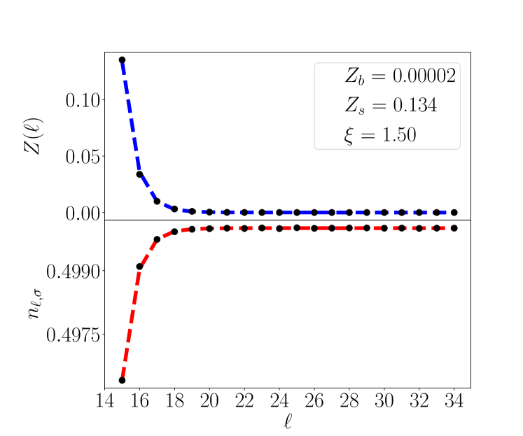
Figure 2: Spatial profile of the quasiparticle residue and electron density per spin across the layers. The last metallic layer is placed at $\ell=14$. The Hubbard repulsion in the metal layers is $U=2$ and in the insulating ones $U=16.828$, and $\delta\mu=-0.9$. The dashed line in the first panel is obtained by the fit, instead in the dashed line in the second panel is obtained through 42. The legend shows the parameter obtained by the fit, where $Z_{s}=R_{s}^{2}$ and $Z_{b}=R_{b}^{2}$ are the value of the metallicity in the first insulating layer and deep in the bulk.

We quantitatively address this question by simulating a metal-Mott interface away from p-h symmetry. More specifically, we study a system of 100 layers where 15 layers are metallic with $U=2$, the value that we use here and in the next section. In Fig. 2 we plot the layer-dependent quasiparticle residue and the electron density per spin starting from the last metallic layer and for $\delta\mu=-0.9$, see Eq. (1). Differently from the p-h symmetric case, the proximity effect is shown also in the electron density, which is not anymore constrained by p-h symmetry. We fit the layer dependent wavefunction renormalisation through the expression:

$$R(\ell) =R_{b}+\big{(}R_{s}-R_{b}\big{)}\,\text{e}^{(\ell-\ell_{*})/\xi}\;,$$ (13)

where $\ell_{*}$ is the index of the first insulating layer and $\xi$ the correlation length. From equation LABEL:fitting_formulas we can obtain the quasiparticle residue, which in standard Gutzwiller is just $Z(\ell)=R(\ell)^{2}$. Instead, the functional form of the density can be deduced, near criticality, by LABEL:fitting_formulas through equation 42 in appendix B.

For $\delta\mu=-0.9$, the first-order Mott transition occurs at ${U_{c}\approx 16.3}$, and $\xi$ diverges as $1/\sqrt{|U-U_{c}|}$ approaching the transition, a typical mean-field exponent. To further confirm the critical properties of the wetting layer, we rescale both the layer coordinate and $Z(\ell)$ as discussed in [33]. Indeed, all data for different values of $U$ collapse on the same curve, as shown in Fig. 3, supporting the wetting critical behaviour, see also Appendix B.

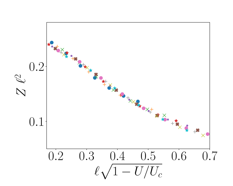
Figure 3: Scaling plot for the quasiparticle residue at $\delta\mu=-0.9$ close to the critical point confirming the mean field exponent $\nu=1/2$.

III Ghost Gutzwiller results

We can readily extend the results of the previous section to the gGut approximation. In the bulk case and for the single band Hubbard model, it has been shown [32] that already with $N_{aux}=3$ one can obtain the Hubbard bands and have a quantitative description of the Mott transition in excellent agreement with the DMFT solution.
We find that moving away from p-h symmetry the transition within gGut remains second-order, even upon increasing the number of auxiliary fermions, as discussed in section IV. We are therefore back to the surface critical behaviour discussed in [33, 35].

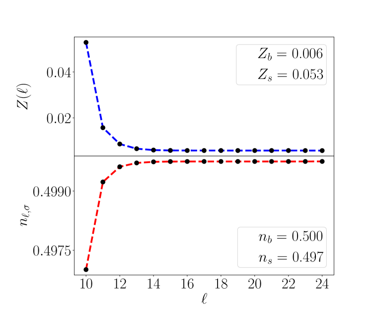
Figure 4: Behaviour of the gGut quasiparticle residue and electron density per spin at $\delta\mu=-0.5$, using $U=14.385$ in the insulating layers. The last metallic layer is $\ell=9$. In the legends are reported the quasiparticle residue and the density in the bulk ($Z_{b}$, $n_{b}$) and in the first insulating layer ($Z_{s}$,$n_{s}$).

We study systems up to 30 layers with $N_{aux}=3$ and find a clear proximity effect both in the quasiparticle residue and the electron density, as shown in Fig. 4.

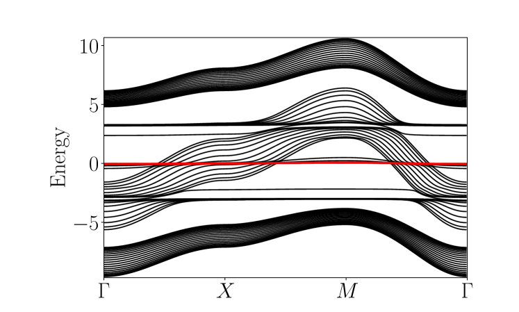
Figure 5: Bands of the quasiparticle Hamiltonian for a slab with 10 metallic layers and 20 Mott insulating ones, at $\delta\mu=-0.5$ and $U=15$ in the insulating layers.

Besides uncovering, as before, the critical behaviour, we can now examine how the presence of the metallic leads affects the quasiparticles in the insulating layers. In Fig. 5, we show the quasiparticle bands along high-symmetry paths of the two-dimensional Brillouin zone, corresponding to the $y$-$z$ plane, in the case with 10 metallic layers out of 30. We observe the following qualitative structure of the figure: some bands cross zero energy, corresponding to the metallic layers, and the others accumulate to form lower and upper Hubbard bands. In particular, a feature that we always find is a set of flat bands pinned at zero energy. We shall thoroughly discuss these zero-energy modes in the Sec. IV, but we anticipate here that they essentially describe spinons, i.e., gapless spin-1/2 neutral excitations. What is remarkable in Fig. 5 is that the spinon band does not shift rigidly with $\delta\mu$ in Eq. (1), as the Hubbard bands instead do, but remains pinned at zero energy, consistently with the spinons being neutral quasiparticles and thus unaffected by the chemical potential.
The spinons thus offer a very simple interpretation of the Kondo proximity effect: at the interface with the metal the spinon reacquires charge and gets promoted into a Kondo resonance narrowly peaked at zero energy. More precisely, the flat band hybridizes with the last metallic layer like in heavy fermion systems, leading to a very narrow band and the opening of small hybrization gaps. To motivate this claim we plot in figure 6 the layer character of the low energy bands of figure 5, showing how the first insulating layer contribute to the dispersive bands.

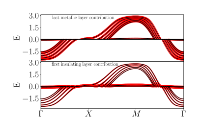
Figure 6: Layer resolved low energy bands of figure 5, the red circles increase in size the more the layer contribute each. Top panel: contribution of the last metallic layer. Bottom panel: contribution of the first insulating layer. The insulating layer contributes to the dispersive bands showing an hybridization between the spinons and metallic bands.

For completeness, in Fig. 7 we plot the layer-resolved spectral function $\mathcal{A}(\omega,\ell)=-\text{Im}\,G(\omega,\ell)/\pi$ for a slab made of five metallic and five insulatinglayers that further highlights the layer evolution of the Kondo peak. We have thus shown that the zero-energy quasiparticle excitations inside the paramagnetic Mott insulator, a simple version of quantum spin liquid, appear at metallic interfaces in the form of a heavy-fermion proximity effect.

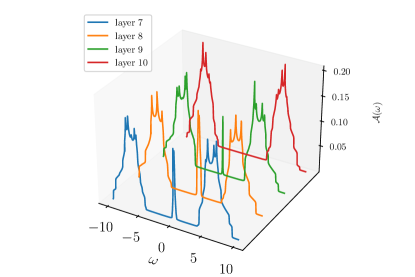
Figure 7: Layer resolved spectral function for $\delta\mu=0.5$ and $U=14.316$ showing how the Kondo peak, always centred at zero frequency, disappears moving away from the interface.

IV Origin of the spinon mode

In this section, we highlight by simple analytical calculations the role played by the zero-energy quasiparticles in the variational optimization, and show that they possess all prerequisites for being legitimately regarded as spinons. Consistently with the slab geometry in Fig. 1, we consider a bulk system on a cubic lattice with periodic boundary conditions.
We start by showing that in gGut the Mott transition is second order also away from p-h symmetry, unlike in Gut or DMFT. In Fig. 8 we show the evolution of the energy, average density per spin and quasiparticle residue, first upon increasing $U$ from the weakly correlated metal (blue solid lines), and then decreasing it from the insulating side (red dashed lines). We observe a metal-insulator coexistence, but, differently from DMFT away from p-h symmetry, the energy does not show any discontinuity in the slope as expected at a first order phase transition. Rather, the behaviour in Fig. 8 resembles the DMFT one at p-h symmetry [34], where there is metal-insulator coexistence but the metal spinodal point coincides with the value of $U$ at which the two energies cross, hence the accidental second-order transition. We mention that a similar disagreement between gGut and DMFT was observed in [38] studying the Mott transition in presence of a magnetic field, which is predicted continuous in gGut and discontinuous in DMFT. Another feature of the bulk gGut solution, in common with the previous slab geometry, is that the quasiparticle bands include dispersing and p-h asymmetric lower and upper Hubbard bands, as well as a flat band pinned at zero energy in the Mott phase that reacquires a narrow dispersion in the correlated metal, see Fig. 9.

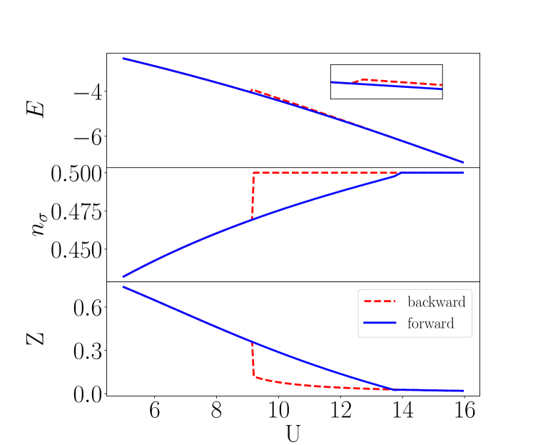
Figure 8: Ground state energy, quasiparticle residue, and density per spin as a function of $U$ in the cubic lattice Hubbard model at $\delta\mu=-1$.

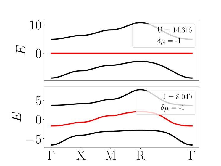
Figure 9: Bands of the quasiparticle Hamiltonian drawn along high-symmetry paths in the Brillouin zone of a cubic lattice for $\delta\mu=-1$. The top panel refers to $U=14.316$ in the Mott insulating phase, while the bottom panel to $U=8.040$ in the correlated metal with preformed Hubbard bands.

To enlighten the role of the zero-energy quasiparticles, we here elaborate on the arguments presented in [38], see also [57]. Specifically, we consider the embedded impurity model with $N_{aux}=3$, sketched in Fig. 10. This is representative of all models with $N_{aux}$ odd, while the case of even $N_{aux}$ will be discussed later. The impurity level is on the right, in blue, shifted up in energy by $-\delta\mu$, with $\delta\mu<0$ in the figure. In the Mott insulator, $U$ overwhelms by far $\delta\mu$ so that the impurity wants to be half-filled, in the figure with a spin-up electron. The positive-energy and negative-energy bath levels, in red, correspond, respectively, to the lower (LHB) and upper (UHB) Hubbard bands, and are hybridised with the impurity by $V_{\text{LHB}}$ and $V_{\text{UHB}}$. The bath level in between, in black, is instead not hybridised with the impurity [32]. At order zero in $V_{\text{LHB}}$ and $V_{\text{UHB}}$, the LHB is full and the UHB empty, as in the figure. However, because of the finite hybridisation, the actual ground state of the impurity+LHB+UHB model, in cyan in Fig. 10, includes other configurations, for instance the impurity empty and one electron on the UHB. We remark that, to maximise the energy gain of the hybridisation, it is preferable that the LHB and UHB are symmetrically located with respect to the impurity level, thus both shifted by $-\delta\mu$, as in the figure.
We denote as $\ket{\Psi_{\sigma}}$ the actual ground state of the impurity+LHB+UHB model, where $\sigma$, $\uparrow$ in the figure, is the $z$-component of the total spin, which is 1/2 in the ground state. One may naïvely argue that the decoupled bath level is fully irrelevant and can be in any configuration, singly occupied, empty or doubly occupied. This is not true however, since Eq. (9) connects the single-particle reduced density matrix of the bath levels with the local single-particle density matrix of the quasiparticles, which, in turn, affects the expectation value of $\mathcal{H}_{*}$ in Eq. (3). One can readily convince oneself that the lowest variational energy is obtained with the decoupled bath level singly-occupied and coupled in a spin-singlet configuration with the impurity+LHU+UHB or, in other words, the wavefunction

$$\ket{\phi} =\frac{\displaystyle\;1\;}{\displaystyle\;\sqrt{2}\;}\,\big{(}\ket{\psi_{\uparrow}}\ket{\Psi_{\downarrow}}-\ket{\psi_{\downarrow}}\ket{\Psi_{\uparrow}}\big{)}\,.$$ (14)

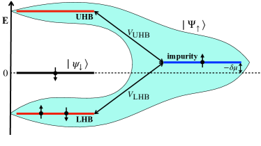
Figure 10: Schematic representation of the effective impurity model in the Mott insulator.

Indeed, let us denote the Fock states of a single level as $\gamma=0$, the empty state, $\gamma=\sigma$, the state with a spin-$\sigma$ electron, and $\gamma=2$, the doubly occupied one, and the Fock states of the impurity+LHB+UHB as $\ket{\gamma_{imp},\gamma_{\text{LHB}},\gamma_{UHB}}$. For large $U$, we can safely assume the trial wavefunction

$$\ket{\Psi_{\sigma}}=\cos\theta\ket{\sigma,2,0}+\frac{\displaystyle\;\sin\theta\;}{\displaystyle\;\sqrt{2}\;}\,\big{(}\ket{0,2,\sigma}+\ket{2,\sigma,0}\big{)}\,,$$ (15)

with $\theta\simeq 0$. Using the spin-singlet configuration in Eq. (14), we find that the occupation numbers of LHB and UHB are spin-independent are read

$$n_{\text{LHB}\sigma} =1-\frac{\displaystyle\;1\;}{\displaystyle\;4\;}\,\sin^{2}\theta\,, n_{\text{UHB}\sigma} =\frac{\displaystyle\;1\;}{\displaystyle\;4\;}\,\sin^{2}\theta\,,$$ (16)

while the impurity is half-filled. We note that Eq. (9) entails that the quasiparticle local density matrix is the p-h transform of the impurity bath one, thus that the impurity LHB and UHB transform, respectively, into the quasiparticle UHB and LHB. Since, for $a=\text{LHB},\text{UHB}$,

$$\bra{\phi}d^{\dagger}_{a\sigma}\,c^{\phantom{\dagger}}_{\sigma}\ket{\phi} =\frac{\displaystyle\;\sin\theta\,\cos\theta\;}{\displaystyle\;2\sqrt{2}\;}\;,$$ (17)

and $n_{a\sigma}(1-n_{a\sigma})=\sin^{2}\theta/4$ are independent of $a$, the wavefunction renormalisation factors are as well, and read [32]

$$R_{a\sigma} =\frac{\displaystyle\;\bra{\phi}d^{\dagger}_{a\sigma}\,c^{\phantom{\dagger}}_{\sigma}\ket{\phi}\;}{\displaystyle\;\sqrt{n_{a\sigma}\,\big{(}1-n_{a\sigma}\big{)}}\;}$$ (18)

$$=\frac{\displaystyle\;2\;}{\displaystyle\;\sin\theta\;}\;\frac{\displaystyle\;\sin\theta\,\cos\theta\;}{\displaystyle\;2\sqrt{2}\;}\simeq\frac{\displaystyle\;1\;}{\displaystyle\;\sqrt{2}\;}\,.$$

The quasiparticle Hamiltonian Eq. (7) is therefore

$$\mathcal{H}^{qp} =\frac{\displaystyle\;1\;}{\displaystyle\;2\;}\,\sum_{\mathbf{k}\sigma}\,\sum_{a,b=\text{LHB},\text{HUB}}{\epsilon}(\mathbf{k})\,d^{\dagger}_{\mathbf{k}a\sigma}\,d^{\phantom{\dagger}}_{\mathbf{k}b\sigma}$$ (19)

$$\qquad-\lambda\,\sum_{\mathbf{k}}\,\big{(}n_{\mathbf{k}\text{LHB}}-n_{\mathbf{k}\text{UHB}}\big{)}$$

$$=\mathcal{H}_{*}-\lambda\,\sum_{\mathbf{k}}\,\big{(}n_{\mathbf{k}\text{LHB}}-n_{\mathbf{k}\text{UHB}}\big{)}\,,$$

plus the flat zero-energy band that, because of Eq. (9) and Eq. (14), is half-filled with equal number of spin up and down quasiparticles. The Hamiltonian in Eq. (19) describes two bands with dispersion

$${\epsilon}_{\mp}(\mathbf{k}) =\frac{\displaystyle\;1\;}{\displaystyle\;2\;}\,\bigg{(}{\epsilon}(\mathbf{k})\mp\sqrt{{\epsilon}(\mathbf{k})^{2}+4\lambda^{2}\;}\,\bigg{)}\,,$$ (20)

and corresponding eigenoperators

$$d^{\phantom{\dagger}}_{\mathbf{k}\,-\,\sigma} =\cos\theta_{\mathbf{k}}\,d^{\phantom{\dagger}}_{\mathbf{k}\text{LHB}\sigma}+\sin\theta_{\mathbf{k}}\,d^{\phantom{\dagger}}_{\mathbf{k}\text{UHB}\sigma}\,,$$ (21)

$$d^{\phantom{\dagger}}_{\mathbf{k}\,+\,\sigma} =-\sin\theta_{\mathbf{k}}\,d^{\phantom{\dagger}}_{\mathbf{k}\text{LHB}\sigma}+\cos\theta_{\mathbf{k}}\,d^{\phantom{\dagger}}_{\mathbf{k}\text{UHB}\sigma}\,,$$

with $\tan 2\theta_{\mathbf{k}}={\epsilon}(\mathbf{k})/2\lambda$. The parameter $\lambda$ in Eq. (19) is a Lagrange multiplier that enforces the self-consistency condition in Eq. (9), namely, that the LHB is almost full and the HUB almost empty. This requires $\lambda\gg t$, thus ${\epsilon}_{-}(\mathbf{k})<0$ and ${\epsilon}_{+}(\mathbf{k})>0$ separated by a gap $2\lambda$, and the ground state $\ket{\Psi_{*}}$ obtained by filling the lowest-energy band. Specifically, the self-consistency Eq. (9) together with Eq. (16) imply, through Eq. (21), that

$$\frac{\displaystyle\;1\;}{\displaystyle\;V\;}\sum_{\mathbf{k}}\,\bra{\Psi_{*}}n_{\mathbf{k}\text{LHB}}\ket{\Psi_{*}} \simeq 2-\frac{\displaystyle\;3t^{2}\;}{\displaystyle\;4\lambda^{2}\;}=2-\frac{\displaystyle\;\sin^{2}\theta\;}{\displaystyle\;2\;}\,,$$ (22)

$$\frac{\displaystyle\;1\;}{\displaystyle\;V\;}\sum_{\mathbf{k}}\,\bra{\Psi_{*}}n_{\mathbf{k}\text{UHB}}\ket{\Psi_{*}} \simeq\frac{\displaystyle\;3t^{2}\;}{\displaystyle\;4\lambda^{2}\;}=\frac{\displaystyle\;\sin^{2}\theta\;}{\displaystyle\;2\;}\,.$$

It follows that $3t^{2}/2\lambda^{2}=\sin^{2}\theta$ and that the variational energy per site is

$$E =\frac{\displaystyle\;1\;}{\displaystyle\;V\;}\,\bra{\Psi_{*}}\mathcal{H}_{*}\ket{\Psi_{*}}+\frac{\displaystyle\;U\;}{\displaystyle\;2\;}\,\bra{\phi}(n-1)^{2}\ket{\phi}$$ (23)

$$\simeq-\frac{\displaystyle\;3t^{2}\;}{\displaystyle\;\lambda\;}+\frac{\displaystyle\;U\;}{\displaystyle\;2\;}\,\sin^{2}\theta=-\frac{\displaystyle\;3t^{2}\;}{\displaystyle\;\lambda\;}+\frac{\displaystyle\;U\;}{\displaystyle\;2\;}\;\frac{\displaystyle\;3t^{2}\;}{\displaystyle\;2\lambda^{2}\;}\,,$$

with minimum at $\lambda=U/2$ and value $E=-3t^{2}/U$. We recall that the half-filled Hubbard model at very large $U$ maps onto a spin-1/2 Heisenberg model

$$H_{\text{Heis}} =J\,\sum_{<ij>}\,\bigg{(}{\bm{S}}_{i}\cdot{\bm{S}}_{j}-\frac{\displaystyle\;1\;}{\displaystyle\;4\;}\bigg{)}\,,$$ (24)

where $J=4t^{2}/U$. We realise that on a cubic lattice the large-$U$ gGut variational energy per site, $E=-3t^{2}/U$, actually $E=-zt^{2}/2U$ for generic lattices with coordination number $z$, reproduces the second term in parenthesis. This represents a big achievement with respect to the standard Gut, which yields a vanishing variational energy [36], and is consistent with the fact that gGut is strictly variational for lattices with infinite coordination, where the term ${\bm{S}}_{i}\cdot{\bm{S}}_{j}$ does not contribute unless breaking the spin $SU(2)$.
If we instead use as starting point of the optimization process the spin-triplet state, e.g., $\ket{\psi_{\uparrow}}\ket{\Psi_{\uparrow}}$, rather than the spin-singlet one in Eq. (14), or the configurations in which the decoupled bath level is empty or doubly occupied, and repeat the previous calculations, we find at large $U$ the same solution as in standard Gut. This, as mentioned above, results in a higher variational energy. The same occurs if the number of auxiliary orbitals, i.e., of bath levels, is $N_{aux}=2$. More generally, the variational solution in the Mott insulator with even $N_{aux}=2M$ coincides with that of $N_{aux}=2M-1$. In other words, the self-consistency condition Eq. (9) effectively provides a strong spin entanglement [38] between the impurity+LHU+UHB and the decoupled bath level, which is forced to lie at zero energy, thus yielding the zero-energy quasiparticle flat-band that, we argue, hosts the spinons.
To support this conjecture, let us study a gGut variational wavefunction with finite magnetisation $m$ per site. Instead of Eq. (14), see Eq. (15), we use as trial wavefunction of the impurity model

$$\ket{\phi} =\cos\theta\,\cos\phi\ket{\psi_{\downarrow}}\ket{\uparrow,2,0}$$ (25)

$$\qquad-\cos\theta\,\sin\phi\ket{\psi_{\uparrow}}\ket{\downarrow,2,0}$$

$$\qquad+\frac{\displaystyle\;\sin\theta\;}{\displaystyle\;2\;}\ket{\psi_{\downarrow}}\big{(}\ket{0,2\uparrow}+\ket{2,\uparrow,0}\big{)}\,,$$

$$\qquad-\frac{\displaystyle\;\sin\theta\;}{\displaystyle\;2\;}\ket{\psi_{\uparrow}}\big{(}\ket{0,2\downarrow}+\ket{2,\downarrow,0}\big{)}\,,$$

which allows for a finite impurity magnetisation that corresponds to the physical one $m$, thus ${n_{\uparrow}-n_{\downarrow}=\cos^{2}2\phi\,\cos^{2}\theta=m}$. We note that the magnetisation of the decoupled bath level coincides with $-m$, which shows that the physical spin is entirely carried by the zero-energy states in the quasiparticle Hamiltonian, whose magnetisation is the p-h transform of the decoupled bath level, thus precisely $m$. Indeed, the choice in Eq. (25) is intentionally done with that purpose, We have confirmed that it reproduces the numerically optimized solution. Correspondingly, the occupation numbers of the LHB and UHB are the same as in Eq. (16), i.e., spin independent. What changes are the expectation values in Eq. (17), which now read

$$\bra{\phi}d^{\dagger}_{\text{UHB}\uparrow}\,c^{\phantom{\dagger}}_{\uparrow}\ket{\phi} =\bra{\phi}d^{\dagger}_{\text{LHB}\downarrow}\,c^{\phantom{\dagger}}_{\downarrow}\ket{\phi}$$ (26)

$$=\cos\phi\;\frac{\displaystyle\;\sin\theta\cos\theta\;}{\displaystyle\;2\;}\;,$$

$$\bra{\phi}d^{\dagger}_{\text{LHB}\uparrow}\,c^{\phantom{\dagger}}_{\uparrow}\ket{\phi} =\bra{\phi}d^{\dagger}_{\text{UHB}\downarrow}\,c^{\phantom{\dagger}}_{\downarrow}\ket{\phi}$$

$$=\sin\phi\;\frac{\displaystyle\;\sin\theta\cos\theta\;}{\displaystyle\;2\;}\;,$$

resulting in the following wavefunction renormalisation factors

$$R_{\text{UHB}\uparrow} =R_{\text{LHB}\downarrow}\simeq\cos\phi\,,$$ (27)

$$R_{\text{LHB}\uparrow} =R_{\text{UHB}\downarrow}\simeq\sin\phi\,.$$

The consequence, as one can readily derive following the former calculations at $m=0$, is a reduction of

$$\bra{\Psi_{*}}\mathcal{H}_{*}\ket{\Psi_{*}}\simeq-\frac{\displaystyle\;3t^{2}\;}{\displaystyle\;\lambda\;}\,\sin^{2}2\phi\,,$$ (28)

and a modified self-consistency condition

$$\frac{\displaystyle\;3t^{2}\;}{\displaystyle\;2\lambda^{2}\;} =\frac{\displaystyle\;\sin^{2}\theta\;}{\displaystyle\;\sin^{2}2\phi\;}\;,$$ (29)

both of which reduce to the previous ones when $\phi=\pi/4$. The variational energy per site is therefore

$$E =-\frac{\displaystyle\;3t^{2}\;}{\displaystyle\;\lambda\;}\,\sin^{2}2\phi+\frac{\displaystyle\;U\;}{\displaystyle\;2\;}\,\sin^{2}2\theta$$ (30)

$$=-3t^{2}\,\sin^{2}2\phi\,\bigg{(}\frac{\displaystyle\;1\;}{\displaystyle\;\lambda\;}-\frac{\displaystyle\;U\;}{\displaystyle\;4\lambda^{2}\;}\bigg{)}\,,$$

with the constraint

$$m =\cos^{2}2\phi\,\cos^{2}\theta=\cos^{2}2\phi\,\bigg{(}1-\frac{\displaystyle\;3t^{2}\;}{\displaystyle\;2\lambda^{2}\;}\,\sin^{2}2\phi\bigg{)}$$ (31)

$$\xrightarrow[\lambda\gg t]{}\cos^{2}2\phi\,,$$

from which we find that the optimal $\lambda=U/2$, as before, and

$$E(m) =-\frac{\displaystyle\;3t^{2}\;}{\displaystyle\;U\;}\,\big{(}1-m^{2}\big{)}\,.$$ (32)

We note that Eq. (32) corresponds precisely to the expectation value per site of the Heisenberg Hamiltonian in Eq. (24) over a state with average spin polarization $\langle S^{z}_{i}\rangle=m/2$ in the limit of infinite coordination-number. In other words, in this limit the variational gGut wavefunction reproduces the exact ground state energy and it does so in a very physical way: the spin polarization is carried just by the quasiparticles of the flat band, justifying our interpretation of them as spinons, whereas the dispersive Hubbard bands remain unpolarized.

We further observe that, even though the spinon band is flat in the quasiparticle Hamiltonian, the variational energy in Eq. (32) is instead compatible with a non-zero dispersion and a finite spinon density-of-states at zero energy. The reason lies in the fact that the spinon and Hubbard bands are not truly independent of each other. Indeed, the spinon polarization does affect the Hubbard bands through (27), and, in turn, the expectation value $\bra{\Psi_{*}}\mathcal{H}_{*}\ket{\Psi_{*}}$. This behaviour is similar to the outcome of conventional Hartree-Fock plus random-phase approximation, and suggests that the inclusion of quantum fluctuations, as done for the Gut using the time-dependent variational principle [44], may explicitly unveil the coupling between the Hubbard bands and the spinon one. In that case, a finite spinon dispersion should appear upon integrating out the high-energy Hubbard bands. Moreover, the finite spinon density-of-states consistent with Eq. (32) suggests that the spinons do have a well-defined Fermi-surface.

V Conclusions

We have shown that the ghost Gutzwiller approximation is able to describe a genuine paramagnetic Mott insulator that hosts neutral spin-1/2 quasiparticles, possibly with their own Fermi surface, the sought-after Anderson’s spinons. Moreover, we have demonstrated that these spinons can be revealed by a proximity effect at the interface between the paramagnetic Mott insulator and a metal. Indeed, the spinons near the interface regain the electron charge and get promoted into bona fide quasiparticles with a narrow dispersion in the directions parallel to the interface that decreases exponentially moving inside the bulk of the Mott insulator. This behavior resembles more a heavy-fermion proximity effect rather than a Kondo-like one that was advocated to interpret the DMFT results [33].
Lastly, we have shown that when the system is allowed to have a finite magnetization $m$, the quadratic energy raise with $m$ is compatible with the spinons having a finite density of state hence a finite dispersion in the Brillouin zone, not accessible at $m=0$.
To unveil the precise form of the spinon dispersion one needs to include quantum fluctuations on top of the variational solution, a work that is currently underway.

Appendix A Gutzwiller variational equations

In this section, we show the gGut equations in the case of a metal-Mott insulator interface. We hereafter impose just the spin-$U(1)$ symmetry corresponding to rotations around the spin $z$axis.
To optimize the wavefunction in 2 we use the Gutzwiller approximation, namely, we use results in the infinite coordination limit and apply them also to finite coordination lattices. We can analytically calculate the expressions of all expectation values over the variational Gutzwiller wavefunction, if we further impose the so-called Gutzwiller constraints [41, 42, 43, 44], which, in the impurity model formulation, read:

$$\braket{\phi(\ell)|\phi(\ell)} =1\,,$$ (33)

$$\bra{\phi(\ell)}d^{\phantom{\dagger}}_{\ell\alpha\sigma}\,d^{\dagger}_{\ell\alpha\sigma}\ket{\phi(\ell)} =\bra{\Psi_{*}}d^{\dagger}_{\ell\bm{r}\beta\sigma}\,d^{\phantom{\dagger}}_{\ell\bm{r}\alpha\sigma}\ket{\Psi_{*}}$$

$$\equiv\Delta_{\alpha\sigma,\beta\sigma}(\ell)\,,$$

where $\Delta_{\alpha\sigma,\beta\sigma}(\ell)$ define a matrix $\hat{\Delta}_{\sigma}(\ell)$. More specifically, the minimization of the energy 3, after imposing Eq. (33) and within the Gutzwiller approximation can be done algebraically by solving the following system of equations:

$$\mathcal{H}_{qp}\ket{\psi_{*}} =E_{qp}\ket{\psi_{*}}~,$$ (34)

$$\bigg{(}\sqrt{\hat{\Delta}_{\sigma}(\ell)\big{(}1-\hat{\Delta}(\ell)_{\sigma}\big{)}\,}\,\bm{V}_{\sigma}(\ell)\bigg{)}_{\alpha} =\sum_{\mathbf{k},\ell^{\prime},\beta}R_{\beta\sigma}(\ell^{\prime})\,\bra{\Psi_{*}}d^{\dagger}_{\ell\mathbf{k}\alpha\sigma}\,d_{\ell^{\prime}\mathbf{k}\beta\sigma}\ket{\Psi_{*}}\,t_{\ell\ell^{\prime}}(\mathbf{k})\,,$$

$$\hat{\lambda}_{\sigma}(\ell) =-\hat{\lambda}^{c}_{\sigma}(\ell)+\frac{\partial}{\partial\hat{\Delta}_{\sigma}(\ell)}\,\bigg{(}\bm{R}_{\sigma}(\ell)\cdot\sqrt{\hat{\Delta}_{\sigma}(\ell)\big{(}1-\hat{\Delta}(\ell)_{\sigma}\big{)}\,}\,\bm{V}_{\sigma}(\ell)+H.c.\bigg{)}\,,$$

$$\mathcal{H}_{imp}(\ell)\ket{\phi(\ell)} =E_{imp}(\ell)\ket{\phi(\ell)}\,,$$

$$\bra{\phi(\ell)}d^{\phantom{\dagger}}_{\ell\alpha\sigma}\,d^{\dagger}_{\ell\alpha\sigma}\ket{\phi(\ell)} =\bra{\Psi_{*}}d^{\dagger}_{\ell\bm{r}\beta\sigma}\,d^{\phantom{\dagger}}_{\ell\bm{r}\alpha\sigma}\ket{\Psi_{*}}=\Delta_{\alpha\sigma,\beta\sigma}(\ell)$$

$$R_{\alpha\sigma}(\ell) =\sum_{\beta}\bigg{(}\sqrt{\hat{\Delta}_{\sigma}(\ell)\big{(}1-\hat{\Delta}(\ell)_{\sigma}\big{)}\,}\,\bigg{)}^{-1}_{\alpha,\beta}\,\bra{\phi(\ell)}c^{\dagger}_{\ell\sigma}\,d^{\phantom{\dagger}}_{\ell\beta\sigma}\ket{\phi(\ell)}\,,$$

where

$$t_{\ell\ell^{\prime}}(\mathbf{k}) =\delta_{\ell\ell^{\prime}}\,{\epsilon}(\mathbf{k})-t\,\big{(}\delta_{\ell^{\prime},\ell+1}+\delta_{\ell^{\prime},\ell-1}\big{)}\,,$$ (35)

$\bm{R}_{\sigma}(\ell)$ and $\bm{V}_{\sigma}(\ell)$ are vectors with components $R_{\alpha\sigma}(\ell)$ and $V_{\alpha\sigma}(\ell)$, respectively, while $\hat{\lambda}_{\sigma}(\ell)$ and $\hat{\lambda}^{c}_{\sigma}(\ell)$ matrices with elements $\lambda_{\alpha\sigma,\beta\sigma}(\ell)$ and $\lambda^{c}_{\alpha\sigma,\beta\sigma}(\ell)$, respectively. The solution of Eq. (34) can be obtained self-consistently starting from a guess for $\bm{R}_{\sigma}(\ell)$ and $\hat{\lambda}_{\sigma}(\ell)$ and iterating the procedure till every equation is satisfied up to the desired accuracy.

Appendix B continuum description for the wetting critical behaviour

In the case of the Gut the Mott transition is first order but we still have a surface critical behaviour, as shown in the main text. In this case, we can find a continuum description to extract the critical behaviour, as done in [35] at p-h symmetry. We write the impurity wavefunction as

$$\ket{\phi(\ell)} =\phi_{0}(\ell)\,\ket{0,2}+\phi_{2}(\ell)\,\ket{2,0}$$ (36)

$$\qquad+\sum_{\sigma}\,\sigma\,\phi_{\sigma}(\ell)\ket{\sigma,-\sigma}\,,$$

where $\ket{\gamma_{imp},\gamma_{bath}}$ is a Fock state of the impurity plus the single bath level. Hereafter, we assume spin-$SU(2)$ symmetry, thus $\phi_{\sigma}(\ell)=\phi_{1}(\ell)$ independent of spin. For the standard Gutzwiller ansatz, we can write the energy functional per site as:

$$E =\frac{\displaystyle\;1\;}{\displaystyle\;N\;}\,\sum_{\ell}\,\bigg{\{}\frac{U_{\ell}}{2}\,\big{(}\phi_{0}(\ell)^{2}+\phi_{2}(\ell)^{2}\big{)}-\delta\mu\,\delta(\ell)\bigg{\}}$$ (37)

$$\qquad+\frac{\displaystyle\;1\;}{\displaystyle\;N\;}\sum_{\ell}\,R^{2}_{\sigma}(\ell)\,{\epsilon}_{\ell}$$

$$\qquad+\frac{\displaystyle\;1\;}{\displaystyle\;N\;}\sum_{\ell}\,\sum_{p=\pm 1}\,\,R_{\sigma}(\ell)\,t_{\ell\ell+p}\,R_{\sigma}(\ell+p)\,,$$

where $N$ is the number of layers and

$${\epsilon}_{\ell} =\frac{\displaystyle\;1\;}{\displaystyle\;\mathcal{A}\;}\,\sum_{\mathbf{k}\sigma}\,\bra{\Psi_{*}}c^{\dagger}_{\ell\mathbf{k}\sigma}\,{\epsilon}(\mathbf{k})\,c^{\phantom{\dagger}}_{\ell\mathbf{k}\sigma}\ket{\Psi_{*}}\,,$$ (38)

$$t_{\ell\ell^{\prime}} =-\frac{\displaystyle\;t\;}{\displaystyle\;\mathcal{A}\;}\,\sum_{\mathbf{k}\sigma}\,\bra{\Psi_{*}}c^{\dagger}_{\ell\mathbf{k}\sigma}\,c^{\phantom{\dagger}}_{\ell^{\prime}\mathbf{k}\sigma}\ket{\Psi_{*}}\,.$$

The Gutzwiller constraints and the equation for $R_{\sigma}(\ell)=R(\ell)$ read:

$$1 =\phi_{0}(\ell)^{2}+\phi_{2}(\ell)^{2}+2\,\phi_{1}(\ell)^{2}\,,$$ (39)

$$n(\ell) =1-\delta(\ell)=2\phi_{2}(\ell)^{2}+2\phi_{1}(\ell)^{2}\,,$$

$$R(\ell)^{2} =\frac{\displaystyle\;4\;}{\displaystyle\;1-\delta(\ell)^{2}\;}\big{(}\phi_{2}(\ell)\,\phi_{1}(\ell)+\phi_{0}(\ell)\,\phi_{1}(\ell)\big{)}^{2}\,.$$

We can choose to express the energy functional using $R(\ell)$ and the doping $\delta(\ell)$ as independent variables, in particular,

$$\phi_{0}(\ell)^{2}+\phi_{2}(\ell)^{2} =\frac{1}{2}\Bigg{(}1-\sqrt{\big{(}1-R(\ell)^{2}\big{)}\big{(}1-\delta(\ell)^{2}\big{)}\,}+\frac{\delta(\ell)^{2}}{\;1-\sqrt{\big{(}1-R(\ell)^{2}\big{)}\big{(}1-\delta(\ell)^{2}\big{)}\,}\;}\Bigg{)}$$ (40)

$$\simeq\frac{1}{2}\Bigg{(}1-\sqrt{1-R(\ell)^{2}\,}+\frac{\delta(\ell)^{2}}{2}\;\frac{\;1+R(\ell)^{2}+\sqrt{1-R(\ell)^{2}\,}\;}{\;1-\sqrt{1-R(\ell)^{2}\,}\;}\,\Bigg{)}\,.$$

Where the last equation is valid in the limit of small doping.
Near the critical point, the quantities in Eq. (38) do not depend appreciably on $\ell$, ${\epsilon}_{\ell}\simeq-{\epsilon}_{\parallel}$ and $t_{\ell\ell\pm 1}\simeq-{\epsilon}_{\perp}/2$, so that, in the continuum limit $\ell\to x$, with continuous $x$, the energy functional reads

$$E =\int{\it dx}\Bigg{\{}\frac{U(x)}{2}\,\Big{[}\phi_{0}(x)^{2}+\phi_{2}(x)^{2}\Big{]}-\epsilon\,R(x)^{2}$$ (41)

$$\qquad\qquad\qquad\quad\;\;+\frac{{\epsilon}_{\perp}}{2}\,\left(\frac{\partial R(x)}{\partial x}\right)^{2}-\delta\mu\,\delta(x)\Bigg{\}}\,,$$

where ${\epsilon}={\epsilon}_{\parallel}+{\epsilon}_{\perp}$, and $\phi_{0}(x)^{2}+\phi_{2}(x)^{2}$ is given by Eq. (40). Solving the Euler-Lagrange equations we can express $\delta(x)$ as a function of R(x):

$$\delta(x)=\frac{4\delta\mu}{U(x)}\frac{1-\sqrt{1-R(x)^{2}}}{1+R(x)^{2}+\sqrt{1-R(x)^{2}}}~.$$ (42)

The solution for $R(x)$ can be found deep in the Mott insulator, where $U(x)=U$ is constant and $R(x)$ and $\delta(x)$ are small. We find:

$$R(x) \simeq\text{e}^{-x/\xi}\;, \delta(x) \simeq\text{sign}(\delta\mu)\,R(x)^{2}$$ (43)

with the correlation length given by

$$\frac{\displaystyle\;1\;}{\displaystyle\;\xi^{2}\;} =\frac{\displaystyle\;1\;}{\displaystyle\;{\epsilon}_{\perp}\;}\,\bigg{(}\frac{\displaystyle\;U\;}{\displaystyle\;4\;}-2{\epsilon}-\frac{\displaystyle\;\delta\mu^{2}\;}{\displaystyle\;U\;}\bigg{)}\,.$$ (44)

We note that $\xi$ diverges at a critical $U=U_{c}$ which shifts to higher values at $\delta\mu\not=0$, as expected.

References

- Savary and Balents [2016] L. Savary and L. Balents, Quantum spin liquids: a review, Reports on Progress in Physics 80, 016502 (2016).
- Broholm et al. [2020] C. Broholm, R. J. Cava, S. A. Kivelson, D. G. Nocera, M. R. Norman, and T. Senthil, Quantum spin liquids, Science 367, eaay0668 (2020), https://www.science.org/doi/pdf/10.1126/science.aay0668 .
- Wen [2013] X.-G. Wen, Topological order: From long-range entangled quantum matter to a unified origin of light and electrons, International Scholarly Research Notices 2013, 198710 (2013), https://onlinelibrary.wiley.com/doi/pdf/10.1155/2013/198710 .
- Sachdev [2018] S. Sachdev, Topological order, emergent gauge fields, and fermi surface reconstruction, Reports on Progress in Physics 82, 014001 (2018).
- Sachdev [2023] S. Sachdev, Quantum Phases of Matter (Cambridge University Press, 2023).
- Anderson [1987] P. W. Anderson, The Resonating Valence Bond State in La2CuO4 and Superconductivity, Science 235, 1196 (1987), https://www.science.org/doi/pdf/10.1126/science.235.4793.1196 .
- Anderson et al. [1987] P. W. Anderson, G. Baskaran, Z. Zou, and T. Hsu, Resonating–valence-bond theory of phase transitions and superconductivity in -based compounds, Phys. Rev. Lett. 58, 2790 (1987).
- Kivelson et al. [1987] S. A. Kivelson, D. S. Rokhsar, and J. P. Sethna, Topology of the resonating valence-bond state: Solitons and high- superconductivity, Phys. Rev. B 35, 8865 (1987).
- Lee et al. [2006] P. A. Lee, N. Nagaosa, and X.-G. Wen, Doping a Mott insulator: Physics of high-temperature superconductivity, Rev. Mod. Phys. 78, 17 (2006).
- Read and Sachdev [1989] N. Read and S. Sachdev, Some features of the phase diagram of the square lattice SU(N) antiferromagnet, Nuclear Physics B 316, 609 (1989).
- Read and Sachdev [1990] N. Read and S. Sachdev, Spin-Peierls, valence-bond solid, and Néel ground states of low-dimensional quantum antiferromagnets, Phys. Rev. B 42, 4568 (1990).
- Hermele et al. [2004] M. Hermele, T. Senthil, M. P. A. Fisher, P. A. Lee, N. Nagaosa, and X.-G. Wen, Stability of spin liquids in two dimensions, Phys. Rev. B 70, 214437 (2004).
- Yang and Li [2023] J. Yang and T. Li, Instability of the (1) spin liquid with a large spinon Fermi surface in the Heisenberg-ring exchange model on the triangular lattice, Phys. Rev. B 108, 235105 (2023).
- Seifert et al. [2024] U. F. P. Seifert, J. Willsher, M. Drescher, F. Pollmann, and J. Knolle, Spin-Peierls instability of the U(1) Dirac spin liquid, Nature Communications 15, 7110 (2024).
- Patel and Trivedi [2019] N. D. Patel and N. Trivedi, Magnetic field-induced intermediate quantum spin liquid with a spinon Fermi surface, Proceedings of the National Academy of Sciences 116, 12199 (2019), https://www.pnas.org/doi/pdf/10.1073/pnas.1821406116 .
- Coldea et al. [2001] R. Coldea, D. A. Tennant, A. M. Tsvelik, and Z. Tylczynski, Experimental Realization of a 2D Fractional Quantum Spin Liquid, Phys. Rev. Lett. 86, 1335 (2001).
- Coldea et al. [2003] R. Coldea, D. A. Tennant, and Z. Tylczynski, Extended scattering continua characteristic of spin fractionalization in the two-dimensional frustrated quantum magnet observed by neutron scattering, Phys. Rev. B 68, 134424 (2003).
- Yamashita et al. [2008] S. Yamashita, Y. Nakazawa, M. Oguni, Y. Oshima, H. Nojiri, Y. Shimizu, K. Miyagawa, and K. Kanoda, Thermodynamic properties of a spin-1/2 spin-liquid state in a -type organic salt, Nature Physics 4, 459 (2008).
- Yamashita et al. [2009] M. Yamashita, N. Nakata, Y. Kasahara, T. Sasaki, N. Yoneyama, N. Kobayashi, S. Fujimoto, T. Shibauchi, and Y. Matsuda, Thermal-transport measurements in a quantum spin-liquid state of the frustrated triangular magnet -(BEDT-TTF)2Cu2(CN)3, Nature Physics 5, 44 (2009).
- Yamashita et al. [2010] M. Yamashita, N. Nakata, Y. Senshu, M. Nagata, H. M. Yamamoto, R. Kato, T. Shibauchi, and Y. Matsuda, Highly Mobile Gapless Excitations in a Two-Dimensional Candidate Quantum Spin Liquid, Science 328, 1246 (2010), https://www.science.org/doi/pdf/10.1126/science.1188200 .
- Yamashita et al. [2011] S. Yamashita, T. Yamamoto, Y. Nakazawa, M. Tamura, and R. Kato, Gapless spin liquid of an organic triangular compound evidenced by thermodynamic measurements, Nature Communications 2, 275 (2011).
- Ribak et al. [2017] A. Ribak, I. Silber, C. Baines, K. Chashka, Z. Salman, Y. Dagan, and A. Kanigel, Gapless excitations in the ground state of , Phys. Rev. B 96, 195131 (2017).
- Yu et al. [2017] Y. J. Yu, Y. Xu, L. P. He, M. Kratochvilova, Y. Y. Huang, J. M. Ni, L. Wang, S.-W. Cheong, J.-G. Park, and S. Y. Li, Heat transport study of the spin liquid candidate , Phys. Rev. B 96, 081111 (2017).
- Gomilšek et al. [2019] M. Gomilšek, R. Žitko, M. Klanjšek, M. Pregelj, C. Baines, Y. Li, Q. M. Zhang, and A. Zorko, Kondo screening in a charge-insulating spinon metal, Nature Physics 15, 754 (2019).
- Chen et al. [2022] Y. Chen, W.-Y. He, W. Ruan, J. Hwang, S. Tang, R. L. Lee, M. Wu, T. Zhu, C. Zhang, H. Ryu, F. Wang, S. G. Louie, Z.-X. Shen, S.-K. Mo, P. A. Lee, and M. F. Crommie, Evidence for a spinon Kondo effect in cobalt atoms on single-layer 1T-TaSe2, Nature Physics 18, 1335 (2022).
- Zhang et al. [2024] Q. Zhang, W.-Y. He, Y. Zhang, Y. Chen, L. Jia, Y. Hou, H. Ji, H. Yang, T. Zhang, L. Liu, H.-J. Gao, T. A. Jung, and Y. Wang, Quantum spin liquid signatures in monolayer 1T-NbSe2, Nature Communications 15, 2336 (2024).
- Norman and Micklitz [2009] M. R. Norman and T. Micklitz, How to Measure a Spinon Fermi Surface, Phys. Rev. Lett. 102, 067204 (2009).
- Kishony and Berg [2021] G. Kishony and E. Berg, Converting electrons into emergent fermions at a superconductor–Kitaev spin liquid interface, Phys. Rev. B 104, 235118 (2021).
- Wagner et al. [2023] N. Wagner, L. Crippa, A. Amaricci, P. Hansmann, M. Klett, E. J. König, T. Schäfer, D. D. Sante, J. Cano, A. J. Millis, A. Georges, and G. Sangiovanni, Mott insulators with boundary zeros, Nature Communications 14, 7531 (2023).
- Wagner et al. [2024] N. Wagner, D. Guerci, A. J. Millis, and G. Sangiovanni, Edge Zeros and Boundary Spinons in Topological Mott Insulators, Phys. Rev. Lett. 133, 126504 (2024).
- Peri et al. [2024] V. Peri, S. Ilani, P. A. Lee, and G. Refael, Probing quantum spin liquids with a quantum twisting microscope, Phys. Rev. B 109, 035127 (2024).
- Lanatà et al. [2017] N. Lanatà, T.-H. Lee, Y.-X. Yao, and V. Dobrosavljević, Emergent Bloch excitations in Mott matter, Phys. Rev. B 96, 195126 (2017).
- Helmes et al. [2008] R. W. Helmes, T. A. Costi, and A. Rosch, Kondo Proximity Effect: How Does a Metal Penetrate into a Mott Insulator?, Phys. Rev. Lett. 101, 066802 (2008).
- Georges et al. [1996] A. Georges, G. Kotliar, W. Krauth, and M. J. Rozenberg, Dynamical mean-field theory of strongly correlated fermion systems and the limit of infinite dimensions, Rev. Mod. Phys. 68, 13 (1996).
- Borghi et al. [2010] G. Borghi, M. Fabrizio, and E. Tosatti, Strongly correlated metal interfaces in the Gutzwiller approximation, Phys. Rev. B 81, 115134 (2010).
- Brinkman and Rice [1970] W. F. Brinkman and T. M. Rice, Application of Gutzwiller’s Variational Method to the Metal-Insulator Transition, Phys. Rev. B 2, 4302 (1970).
- Bauer and Hewson [2007] J. Bauer and A. C. Hewson, Field-dependent quasiparticles in the infinite-dimensional Hubbard model, Phys. Rev. B 76, 035118 (2007).
- Guerci et al. [2019] D. Guerci, M. Capone, and M. Fabrizio, Exciton Mott transition revisited, Phys. Rev. Mater. 3, 054605 (2019).
- Gutzwiller [1963] M. C. Gutzwiller, Effect of correlation on the ferromagnetism of transition metals, Phys. Rev. Lett. 10, 159 (1963).
- Gutzwiller [1965] M. C. Gutzwiller, Correlation of electrons in a narrow band, Phys. Rev. 137, A1726 (1965).
- Bünemann et al. [1998] J. Bünemann, W. Weber, and F. Gebhard, Multiband Gutzwiller wave functions for general on-site interactions, Phys. Rev. B 57, 6896 (1998).
- Fabrizio [2007] M. Fabrizio, Gutzwiller description of non-magnetic Mott insulators: Dimer lattice model, Phys. Rev. B 76, 165110 (2007).
- Lanatà et al. [2015] N. Lanatà, Y. Yao, C.-Z. Wang, K.-M. Ho, and G. Kotliar, Phase Diagram and Electronic Structure of Praseodymium and Plutonium, Phys. Rev. X 5, 011008 (2015).
- Fabrizio [2017] M. Fabrizio, Quantum fluctuations beyond the Gutzwiller approximation, Phys. Rev. B 95, 075156 (2017).
- Lee and Yee [2017] J. Lee and C.-H. Yee, Interfaces in coexisting metals and mott insulators, Phys. Rev. B 95, 205126 (2017).
- Frank et al. [2021] M. S. Frank, T.-H. Lee, G. Bhattacharyya, P. K. H. Tsang, V. L. Quito, V. Dobrosavljević, O. Christiansen, and N. Lanatà, Quantum embedding description of the Anderson lattice model with the ghost Gutzwiller approximation, Phys. Rev. B 104, L081103 (2021).
- Lanatà [2022] N. Lanatà, Operatorial formulation of the ghost rotationally invariant slave-boson theory, Phys. Rev. B 105, 045111 (2022).
- Mejuto-Zaera and Fabrizio [2023] C. Mejuto-Zaera and M. Fabrizio, Efficient computational screening of strongly correlated materials: Multiorbital phenomenology within the ghost Gutzwiller approximation, Phys. Rev. B 107, 235150 (2023).
- Guerci et al. [2023] D. Guerci, M. Capone, and N. Lanatà, Time-dependent ghost Gutzwiller nonequilibrium dynamics, Phys. Rev. Res. 5, L032023 (2023).
- Lee et al. [2023a] T.-H. Lee, C. Melnick, R. Adler, N. Lanatà, and G. Kotliar, Accuracy of ghost-rotationally-invariant slave-boson theory for multiorbital Hubbard models and realistic materials, Phys. Rev. B 108, 245147 (2023a).
- Lee et al. [2023b] T.-H. Lee, N. Lanatà, and G. Kotliar, Accuracy of ghost rotationally invariant slave-boson and dynamical mean field theory as a function of the impurity-model bath size, Phys. Rev. B 107, L121104 (2023b).
- Mejuto-Zaera [2024] C. Mejuto-Zaera, Quantum embedding for molecules using auxiliary particles – the ghost gutzwiller ansatz, Faraday Discuss. , Advance Article (2024).
- Lee et al. [2024] T.-H. Lee, C. Melnick, R. Adler, X. Sun, Y. Yao, N. Lanatà, and G. Kotliar, Charge self-consistent density functional theory plus ghost rotationally invariant slave-boson theory for correlated materials, Phys. Rev. B 110, 115126 (2024).
- Lipowsky [1982] R. Lipowsky, Critical surface phenomena at first-order bulk transitions, Phys. Rev. Lett. 49, 1575 (1982).
- Del Re et al. [2016] L. Del Re, M. Fabrizio, and E. Tosatti, Nonequilibrium and nonhomogeneous phenomena around a first-order quantum phase transition, Phys. Rev. B 93, 125131 (2016).
- de Gennes [1985] P. G. de Gennes, Wetting: statics and dynamics, Rev. Mod. Phys. 57, 827 (1985).
- Guerci [2019] D. Guerci, Beyond simple variational approach for strongly correlated electron systems, Ph.D. thesis, International School for Advanced Stusies, SISSA (2019).