PolSAM: Polarimetric Scattering Mechanism Informed Segment Anything Model
Abstract
PolSAR data presents unique challenges due to its rich and complex characteristics. Existing data representations, such as complex-valued data, polarimetric features, and amplitude images, are widely used. However, these formats often face issues related to usability, interpretability, and data integrity. While most feature extraction networks for PolSAR attempt to address these issues, they are typically small in size, which limits their ability to effectively extract features. To overcome these limitations, we introduce the large, powerful Segment Anything Model (SAM), which excels in feature extraction and prompt-based segmentation. However, SAM’s application to PolSAR is hindered by modality differences and limited integration of domain-specific knowledge. To address these challenges, we propose the Polarimetric Scattering Mechanism-Informed SAM (PolSAM), which incorporates physical scattering characteristics and a novel prompt generation strategy to enhance segmentation performance with high data efficiency. Our approach includes a new data processing pipeline that utilizes polarimetric decomposition and semantic correlations to generate Microwave Vision Data (MVD) products, which are lightweight, physically interpretable, and information-dense. We extend the basic SAM architecture with two key contributions: The Feature-Level Fusion Prompt (FFP) module merges visual tokens from the pseudo-colored SAR image and its associated MVD, enriching them with supplementary information. When combined with a dedicated adapter, it addresses modality incompatibility in the frozen SAM encoder. Additionally, we propose the Semantic-Level Fusion Prompt (SFP) module, a progressive mechanism that leverages semantic information within MVD to generate sparse and dense prompt embeddings, refining segmentation details. Experimental evaluation on the newly constructed PhySAR-Seg datasets shows that PolSAM outperforms existing SAM-based models (without MVD) and other multimodal fusion methods (with MVD). The proposed MVD enhances segmentation results by reducing data storage and inference time, outperforming other polarimetric feature representations. The source code and data will be publicly available at https://github.com/XAI4SAR/PolSAM.
Index Terms:
PolSAR terrain segmentation, segment anything model, physical scattering characteristic, prompt-based fusion learning.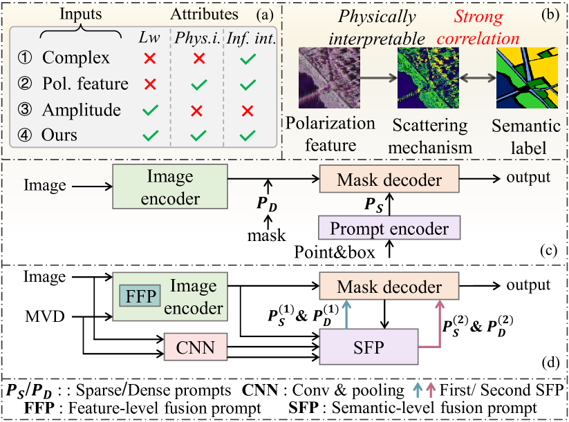
I Introduction
Polarimetric Synthetic Aperture Radar (PolSAR) provides rich polarization features, enabling detailed terrain and ground target representation for applications like land-cover segmentation with enhanced accuracy and feature discrimination [1, 2]. Recently, deep learning-based methods for PolSAR image segmentation have gained traction, typically reformatting PolSAR data into specific input types and designing tailored neural networks to extract both image and polarimetric features [3, 4, 5, 6]. Common representations include complex-valued inputs [7], model-based polarimetric features [8, 9, 6], and amplitude images [10], processed using architectures like complex-valued neural networks (CVNNs) [11, 12], convolutional neural networks (CNNs) [3, 6, 4], Transformers [13], and graph neural networks (GNNs) [14, 15]. However, these input formats face challenges in usability, interpretability, and data integrity, while these models are relatively small, limiting their representational capacity.
As illustrated in Fig. 1(a), complex-valued inputs retain the complete information of PolSAR data but require significantly high storage capacity. Furthermore, their processing necessitates the use of specialized CVNNs, which introduces additional computational complexity and weakens interpretability. This constraint also limits the applicability of existing large-scale vision models, as they are typically designed to handle real-valued data, making the integration of complex-valued inputs more challenging. Model-based polarimetric features enhance the interpretability of complex-valued PolSAR data, allowing for effective integration with popular deep learning architectures such as CNNs, Transformers, and GNNs, however, these features are also high-dimensional. The most widely used format is the 8-bit quantized amplitude PolSAR image, aligned with photographic conventions for compatibility with existing deep learning models. Nevertheless, this approach sacrifices the rich polarimetric features, leading to significant information loss. Investigating a user-friendly input format for PolSAR data that retains integrated polarimetric information is vital in deep learning applications.
In PolSAR image segmentation, the challenges discussed above are further intensified by the limited availability of data. This limitation is particularly pronounced in networks with fewer parameters, as they often fail to extract sufficient information from the input data. A common solution is to transfer knowledge from pre-trained models [16], but the high dimensionality of polarimetric features often makes them incompatible with standard image representations [17]. Although CVNNs have twice the number of parameters compared to traditional real-valued networks, the lack of effective pre-trained models limits their utility. In data-scarce scenarios, CVNNs often struggle to converge, further undermining their practical applicability [18, 19]. While various advanced architectures have been proposed to mitigate these challenges, the inherent limitations of small network sizes hinder their ability to effectively extract relevant features. Additionally, the diversity of PolSAR datasets, variations in scattering mechanisms, and differences in imaging conditions complicate the development of models capable of delivering robust performance across diverse scenarios [6].
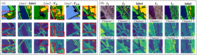
To address these challenges, this work focuses on designing an efficient input format for PolSAR data that integrates Pauli pseudo-colored images with inherent scattering properties of PolSAR, preserving the core polarimetric features crucial for analysis. Previous studies [13, 20] have demonstrated the critical role of scattering mechanisms in PolSAR analysis. As shown in Fig. 1(b), we optimize the scattering properties into a compact image format, reducing storage requirements while providing intuitive physical interpretability. Moreover, specific scattering patterns basically correspond to particular land cover categories, highlighting a strong correlation with semantic label information. With this foundation, we aim to create a generalized segmentation framework for PolSAR image that leverages the robust capabilities of existing large vision models. This approach seeks to bridge the gap between the unique characteristics of PolSAR data and the good generalization ability of advanced large vision models, enabling broader applications and improved usability for non-expert users.
Building on these insights, we introduce the Segment Anything Model (SAM) [21], as shown in Fig. 1(c). First, SAM leverages its large-scale architecture and robust data processing capabilities to achieve efficient and precise segmentation across diverse image content, making it a promising pre-trained foundation model for PolSAR applications. Second, SAM’s prompt-based segmentation mechanism effectively incorporates high-level external prompts, guiding the model to focus on relevant features. This capability is particularly well-suited for compact, high-level scattering mechanism data, providing semantic guidance to enhance segmentation accuracy.
Overall, we propose the Polarimetric Scattering Mechanism-Informed SAM (PolSAM). We first introduce a novel data product, Microwave Vision Data (MVD), which represents compact scattering mechanism classifications. Based on the above description, MVD is lightweight, physically interpretable, and information-dense. Then, to integrate physical scattering properties into SAM, we use two key modules, as shown in Fig. 1(d). The Feature-Level Fusion Prompt (FFP) module first merges patch embeddings from the Pauli decomposition-based pseudo-colored image and MVD, enhancing their interaction before feeding into the SAM encoder. Dedicated adapters in each encoder layer address modality incompatibility in the frozen SAM encoder, fostering feature complementarity. The Semantic-Level Fusion Prompt (SFP) module, second, refines semantic guidance for segmentation through a two-stage process. First, it integrates input features with encoder outputs; then, it aligns the fused representations with high-level semantic prompts, boosting segmentation performance.
Our contributions are as follows:
-
1.
We propose a novel processing pipeline for PolSAR data, focusing on generating user-friendly, physically interpretable, and information-dense MVD products. These lightweight data products effectively leverage the strong correlation between scattering mechanisms and semantics to assist in terrain segmentation of PolSAR data.
-
2.
We propose PolSAM, a SAM-based PolSAR segmentation method that combines PolSAR domain-specific knowledge with SAM’s strengths to improve efficiency and accuracy. PolSAM includes FFP, which fuses Pauli pseudo-colored images and MVD embeddings for better feature complementarity, and SFP, which uses a two-level design to refine semantic prompts through enhanced input and high-level semantic feature interaction.
-
3.
Experiments on two newly constructed PhySAR-Seg datasets confirm that PolSAM outperforms existing SAM-based models and multimodal fusion methods. The sparse and dense prompts generated by our approach capture essential semantic relevance, delivering precise guidance for segmentation tasks. Additionally, the integration of MVD reduces data storage requirements, offering a more efficient alternative to conventional polarimetric representations.
II Related Works
II-A Deep learning based PolSAR image analysis
Deep learning techniques have become essential in PolSAR image analysis, leveraging their advanced information processing capabilities to improve segmentation performance [3, 4, 5, 6]. Currently, widely used methods include CNNs or Transformer-based architectures, graph neural networks (GNNs), and complex-valued neural networks (CVNNs). The inputs processed by these methods can be broadly classified into three categories: complex-valued data, model-based polarimetric features, and simple amplitude data.
As shown in Fig. 1(a), ”✓” denotes an affirmative indicator, ”✕” denotes a negative indicator. Complex-valued data is mainly processed using CVNNs [7, 11, 12]. Clearly, this approach satisfies information integrity (Inf. int.), but it requires high storage and computational resources, making it not lightweight (Lw), while also lacking physical interpretability (Phys. i.). Polarimetric features (Pol. feature), which mainly include Pauli decomposition-based features [8, 22], polarization coherence matrix [9, 23, 24, 17], polarization covariance matrix [6, 25], and scattering features extracted from traditional polarization decomposition methods such as Cloude-Pottier, H/A/Alpha decomposition, Freeman-Durden three-component decomposition, and Yamaguchi four-component decomposition, provide physically interpretable and relatively rich information. These features enhance the ability of deep learning models to interpret PolSAR data [26, 27, 28] . However, they are remain high-dimensional, resulting in high storage and computational costs, making them not lightweight. In comparison, amplitude data, typically represented as 8-bit quantized grayscale images or pseudo-colored images visualized using different polarization modes (HH, HV, VH), is lightweight but suffers from significant information loss and lacks physical interpretability [10]. In summary, these methods face challenges in simultaneously achieving lightweight representation, physical interpretability, and information richness.
Polarimetric features and amplitude data formats can both be processed using networks such as CNNs, Transformers, and GNNs. CNNs and Transformers aim to capture fundamental structural and texture details by enhancing polarization feature representation through advanced techniques [3, 6, 4, 29, 13, 24]. GNNs optimize spatial relationships in PolSAR images by modeling complex spatial dependencies and integrating multi-scale information [30, 27, 31]. Although CNN-based methods effectively utilize polarization features and GNNs capture spatial correlations, these networks often require task-specific designs and training from scratch, limiting their scalability and generalization compared to more general models. Additionally, their computational efficiency still needs improvement.
It is worth noting that existing deep learning models do not directly process the classification results of scattering mechanisms but instead focus on scattering features extracted by traditional decomposition methods. The MVD product we propose represents the classification results of scattering mechanisms, providing higher-level physical information that not only offers better physical interpretability but also has a strong correlation with semantic information. As shown in Fig. 1(a), ours, which combines MVD with Pauli pseudo-colored images, achieves a lightweight, user-friendly representation while preserving physical interpretability and information integrity.
II-B SAM Implementation in Segmentation
The SAM model has demonstrated considerable success in segmentation tasks, primarily due to its large model size, which enables powerful feature extraction and broad applicability. Additionally, its flexible prompt-based segmentation mechanism allows it to effectively handle external high-level prompt information [32, 33, 34, 35]. This versatility has driven adoption across diverse domains, including natural images [33, 32, 36], medical imaging [34, 35, 37, 38, 39], and remote sensing [40, 41, 42, 43]. In medical imaging and remote sensing, where modality differences necessitate tailored approaches, researchers have adapted SAM with specialized adapter techniques [34, 41, 10]. Further refinements, such as integrating text prompts within segmentation modules, have also enhanced its performance [37]. For natural images, innovations explore the use of a multi-modal encoder that combines visual and linguistic information to generate prompt embeddings [44], while PA-SAM [45] introduces a prompt-driven adapter to enhance SAM’s mask quality by refining sparse and dense prompt features. Altogether, these adaptations highlight SAM’s capacity for domain-specific adjustments, extending its applications across diverse image types.
PolSAR data’s scattering mechanism classification results are high-level compared to polarimetric and scattering features, and SAM’s strengths are well-suited to address the challenges we previously outlined. However, despite many of the above methods effectively adjusting SAM, it still faces challenges when applied to PolSAR images, mainly due to modality differences and the inability to integrate domain-specific knowledge. For this, our model introduces two specialized prompt learning modules: one enhances feature complementarity through early-stage fusion of SAR and MVD embeddings, while the other generates precise sparse and dense prompts through a two-level fusion of features and semantic context, effectively guiding the decoder in the segmentation process.
III PhySAR-Seg Dataset
Current PolSAR datasets either rely on quantized amplitude images and pseudo-colored polarization feature images, which lack rich scattering characteristics and physical interpretability, or store complex information, leading to high storage demands. To address these challenges, we propose a novel PolSAR image processing pipeline for constructing the PhySAR-Seg dataset. This dataset is designed to preserve the physical scattering mechanisms in PolSAR images, ensuring both physical interpretability and information integrity, while providing user-friendly, storage-efficient data with strong correlation to meaningful semantic information.
The main innovation in this pipeline is the construction of Microwave Vision Data (MVD), which is defined as a novel representation of PolSAR data. It reflects physical interpretability scattering mechanism and its visual attributes for intuitive understanding. MVD offers several advantages over traditional PolSAR image datasets. First, MVD offers lightweight storage, ensuring high efficiency for large-scale data processing, making it user-friendly. Second, it is both visually and physically interpretable, offering an intuitive visualization of electromagnetic features and a representation of scattering mechanisms with distinct physical meaning. By combining MVD with Pauli pseudo-colored images, we create a more comprehensive dataset. These attributes enhance the efficiency of the PhySAR-Seg dataset, offering deeper insights into both object and terrain characteristics. Details of the processing pipeline and dataset are provided below.
III-A PhySAR-Seg Dataset Processing Pipeline
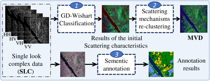
The dataset processing pipeline involves three key steps: (1) Polarimetric decomposition and unsupervised GD-Wishart classification of PolSAR images; (2) MVD generation by re-clustering the physical scattering mechanisms based on semantic correlations; and (3) Manual annotation. Fig. 2 illustrates the entire process, using the PhySAR-Seg-1 dataset as an example.
In the first step, the pseudo-colored image is generated from the original single look complex (SLC) data through the Pauli decomposition algorithm, where three components are extracted and assigned to the RGB channels, respectively [46]. Then, the SLC data is processed using the GD-Wishart classification algorithm [47], yielding initial clustering results. The targets are categorized into three classes: odd-bounce, double-bounce, and volume. Notably, in practical experiments, double-bounce scattering is relatively rare, represented by only one class, while the other categories are further divided into five sub-classes each.
To make MVD more closely aligned with semantic information, we re-cluster the scattering classes. Without altering the primary scattering mechanism categories, we re-group the sub-classes within each category based on their semantic correlations. Apart from the three fundamental scattering types, the dataset may include mixed classes and an ’others’ category. The ’others’ category often contains pixels that lack fixed scattering characteristics, typically appearing at boundaries. We then color the classes based on the final clustering results, visualize the data, and save it. This process allows us to generate MVD, which offers a compact yet informative representation of physical scattering mechanisms. MVD efficiently supports large-scale data processing while providing a clear and intuitive visualization of the electromagnetic properties of objects and terrain. By preserving the physical meaning of these scattering mechanisms, MVD not only optimizes storage and processing but also enhances the clear physical interpretability of the dataset for further analysis.
III-B Datasets Description
Based on the Dataset Processing Pipeline outlined above, we constructed two PhySAR-Seg datasets, each comprising pairs of pseudo-colored and MVD images. These datasets are lightweight, physical interpretable, with scattering mechanisms that have clear physical meanings and exhibit certain correlations with semantic information. Their comprehensive representation capabilities provide a solid foundation for evaluating our proposed method, ensuring that the segmentation model can be effectively trained and assessed on diverse and meaningful data.
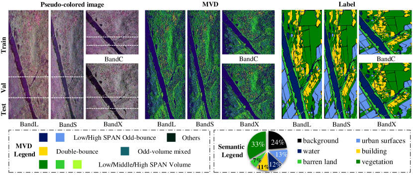
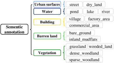
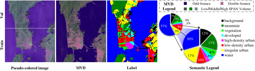
The PhySAR-Seg-1 dataset is sourced from [48]. For our experiments, we use the L, S, C, and X bands, all covering the same geographic region. The L, S, and C bands have a resolution of 0.5 m, while the X band has a resolution of 1.0 m. Fig. 3 provides an overview of the dataset, showcasing the pseudo-colored images, MVD, and label maps, along with both the MVD and semantic legends. In the MVD legend, colors within the same hue represent consistent scattering types, with lighter shades corresponding to higher SPAN values. The semantic legend displays the proportions of the five final terrain classes, clearly illustrating their distribution across the dataset. Initially, the dataset contains 14 land cover types, which we merge into five categories: urban surfaces, water, buildings, barren land, and vegetation, as shown in Fig. 4. A brief note is that we calculate the MVD for each of the four bands. Upon comparison, the X band shows the best performance. Since all bands cover the same region and capture similar scattering mechanisms, we register the X-band MVD to the other three bands to generate the final result. The segmented dataset comprises 2,866 image pairs of pseudo-colored MVD, each with 512 512 pixels. We divide the data from each band into training, validation, and test sets in a 6:2:2 ratio, following the dashed lines shown in Fig. 3. This approach ensures that data from the same geographic region in different bands is allocated to the same set, preventing any overlap between the training, validation, and test sets.
The PhySAR-Seg-2 dataset is sourced from [49] and is based on spaceborne C-band data. We also obtain MVD according to the method in Fig. 2, and labels are obtained through manual annotation, resulting in a total of seven categories excluding the background. Fig. 5 provides an overview of the dataset, including pseudo-colored images, MVD, and their corresponding semantic labels. Due to the limited number of samples in the dataset, we only partition the data into a training set and a validation set in a 6:4 ratio, as indicated by the dashed line in the figure. Given the substantial presence of water in the dataset, we strategically remove pure water samples from the segmented 512 512 images to maintain a balance among categories. After this adjustment, 1,110 images remain, with 668 allocated to the training set and 442 to the validation set. The semantic legend clearly indicates the category distribution before and after processing.
IV The Proposed Method
IV-A Revisiting SAM
The SAM introduces an innovative prompt-based architecture for diverse segmentation tasks. It consists of three main components: the image encoder (), the prompt encoder (), and the mask decoder (). The image encoder extracts high-dimensional feature maps from the input image, which serve as the foundation of SAM’s segmentation capability. The prompt encoder plays a key role by accepting flexible inputs, such as sparse prompts (, e.g., points or bounding boxes), dense prompts (, e.g., masks), and text. These prompts guide the model to focus on specific regions of interest and are transformed into embeddings that integrate with the image features. Finally, the mask decoder fuses both the sparse and dense embeddings with the image features to produce the final segmentation mask. This approach enables SAM to handle diverse segmentation challenges effectively without task-specific fine-tuning. It is a versatile and robust solution for a wide range of scenarios. This can be mathematically represented as follows:
| (1) | ||||
where represents the input image, is the image feature map extracted by the image encoder. , represent the sparse prompt embeddings and dense prompt embeddings. is the final segmentation mask produced by the mask decoder.
Building on the success of SAM in the segmentation field, we adopt its image encoder and mask decoder as the backbone of our segmentation network, keeping the encoder frozen. Inspired by SAM’s prompt-based mechanism, which relies on geometric prompts such as points, boxes, or masks, we propose a novel approach that autonomously generates semantic prompts. By incorporating domain-specific cues, our method produces both sparse and dense semantic prompts, enabling the model to effectively leverage task-specific and data-specific information for enhanced segmentation performance. The detailed structure is described below.
IV-B PolSAM Overview
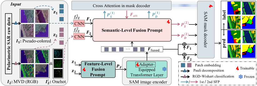
The overview of our proposed PolSAM is illustrated in Fig. 6. We adopt the SAM image encoder () and mask decoder (), keeping their original structures unchanged. Pseudo-colored images offer rich texture details and strong visual representation, while MVD captures scattering mechanisms and conveys semantic information. To effectively exploit and integrate these data-specific features, we propose the Feature-Level Fusion Prompt (FFP) module, placed before the image encoder to fuse features from both inputs for a more comprehensive representation. Additionally, to address data modality incompatibility and better adapt the encoder to PolSAR data, we introduce trainable adapter modules into each layer of the frozen image encoder, enhancing feature representation and segmentation performance.
To provide effective semantic prompts to the decoder, we designed a progressive Semantic-Level Fusion Prompt (SFP) module. Each level targets different aspects of key information, enabling nuanced semantic integration. The process is described by the following equations:
| (2) | ||||
where, and represent the FFP and SFP modules, respectively. denote the pseudo-colored image, and represent MVD in RGB and one-hot form respectively. In the following sections, we will analyze each module in details.
IV-C Feature-Level Fusion Prompt
The design of FFP follows the concept proposed in [50], where a lightweight module with convolutions is inserted into the beginning of the image encoder. In this context, the pseudo-colored image and MVD image are denoted as and , respectively, with their corresponding patch embeddings represented by and . Given the distinct characteristics of these two inputs, is closely related to local details and texture in the image, while reflects the scattering mechanism, which is more related to semantic information. Therefore, enhancing the spatial resolution of is essential to emphasize local details, whereas undergoes direct dimensionality reduction to retain its global semantic features.
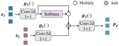
Specifically, as shown in Fig. 7, FFP first takes and as input and performs dimension reduction using 11 convolutions to obtain the latent features for each input. The latent features of are then processed with a Softmax activation across spatial dimensions to emphasize important regions, followed by a multiplication operation to enhance those areas. Subsequently, the fusion features are projected back to their original dimension using 11 convolutions, yielding the initial fusion prompt at the feature level. Here, we use , , and to represent the three convolution layers. Therefore, the fusion prompt can be derived as:
| (3) | ||||
IV-D Adapter-Equipped Image Encoder
The previous is then added by and to input to the pre-trained image encoder. The encoder backbone is frozen during training and we apply the adapter technology proposed in [34] within each layer of the image encoder to adapt the feature extraction. In this way, the fusion prompt and the adapters are learned to satisfy the complementarity of different inputs by fine-tuning only a few parameters. Thus, we can detail the acquisition of as presented in Equation (2):
| (4) |
IV-E Semantic-Level Fusion Prompt
Inspired by SAM’s promptable mechanism, we propose a novel SFP module. This module automatically generates sparse and dense prompt embeddings to provide semantic guidance for segmentation. The SFP module features a two-level progressive structure aimed at optimizing feature integration and enhancing semantic representation. This design ensures a balanced extraction of unique and complementary information from different inputs, leading to a refined understanding that enriches the segmentation process. By progressively refining feature interactions, the SFP module significantly improves the model’s ability to generate precise and contextually aware segmentation results.
First, the pseudo-colored images are processed using a basic convolutional block and two pooling layers to obtain the feature embedding , which is represented by , as shown in Fig. 6. Considering the strong correlation between MVD and semantic labels, for MVD, we directly adopt the CNN network from the SAM prompt encoder used for processing mask prompts. This layer sequentially downsamples the input through three convolution layers, with intermediate normalization and activation functions, reducing the input channels and mapping the final output to the target embedding dimension. To ensure that the semantic prompts are not affected by color encoding, we directly use the one-hot form of the MVD, denoted as . We then obtain the feature embedding , represented by . The features and have the same dimension as . The above can be denoted as:
| (5) |
The proposed SFP is a progressive process, with two levels implemented using a shared module. To clarify, we denote them as SFP-1 and SFP-2. As shown in Fig. 6, each level of the SFP module receives three inputs, denoted as . The inputs of the SFP-1 are the single input embedding and , together with the fused feature from encoder . It outputs the initial sparse and dense prompt . Then, to make the semantic prompts more specific, SFP-2 combines the single-input features and the fusion features in an additive manner, and interacts with the semantic features after the mask decoder attention layer to generate the final sparse and dense prompt , and . The process can be denoted as:
| (6) | ||||
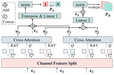
The details of SFP is shown in Fig. 8. Given three arbitrary inputs of , the channel feature split is applied to obtain two feature groups with identical dimensions of , denoted as , , respectively. It is realized by a linear layer to increase the dimension from to . By exchanging the query and value, two groups of enhanced features can be obtained with cross-attention modules, denoted as and , with the dimension of . Then, the sparse prompt and dense prompt are generated separately with the following operations:
| (7) | ||||
where , , and denote the normalization, concatenation, and dimension transformation, respectively. The linear mappings and aim to map the dimension from to , from to , respectively.
From the above descriptions, we can find that SFP module aims to fuse different inputs interactively so that the information is enriched to a certain extent. The two cross-attention modules consider different inputs as the query to obtain the attention weight for feature enhancement. In the SFP-1, , , and are corresponding to , , and . To this end, and demonstrate that the fusion features for segmentation() is enhanced by the single-input features, while and indicate the remarkable single-input features concerned by fusion information. The initial sparse and dense semantic prompts pass through the cross-attention module in the mask decoder to output , which represents high-level semantic features. To this end, in the SFP-2, , and , indicates the result of the mutual enhancement between the fusion information and high-level semantic features.
The significance of the SFP module lies in its ability to enhance feature representation through interactive fusion, progressively refining semantic prompts. This ensures that critical details from each input are preserved while enriching the overall feature space. Furthermore, the mutual enhancement between fused information and high-level semantic features further refines the model’s understanding of feature semantics, leading to improved segmentation results.
| Models | IoU Per Category (%) | Overall Metrics (%) | |||||||
|---|---|---|---|---|---|---|---|---|---|
| BK | Urban surfaces | Water | Building | Barren land | Vegetation | mAcc | mF1 score | mIoU | |
| HQ-SAM[36] | 22.05 | 4.92 | 10.76 | 1.05 | 1.01 | 27.34 | 31.49 | 25.70 | 11.19 |
| SAM-LST[35] | 32.26 | 60.20 | 79.60 | 57.80 | 54.73 | 66.14 | 72.72 | 72.70 | 58.45 |
| Personalize-SAM[32] | 44.65 | 65.12 | 83.99 | 60.93 | 73.29 | 69.8 | 78.26 | 79.39 | 66.30 |
| Mobile-SAM[33] | 22.91 | 52.09 | 77.28 | 42.85 | 44.24 | 55.62 | 64.18 | 64.84 | 49.17 |
| RSAM-Seg[41] | 49.55 | 69.32 | 85.63 | 66.15 | 74.60 | 73.23 | 81.18 | 81.67 | 69.75 |
| PolSAM(w/o MVD) | 51.22 | 69.64 | 86.45 | 68.98 | 78.52 | 76.21 | 82.62 | 83.37 | 71.84 |
| \hdashlineMMSFormer[51] | 46.19 | 68.79 | 85.14 | 63.35 | 67.57 | 72.64 | 79.52 | 80.03 | 67.28 |
| SFAF-MA[52] | 54.29 | 73.03 | 87.56 | 69.41 | 77.07 | 76.99 | 83.67 | 84.33 | 73.06 |
| GMNet[53] | 45.41 | 65.11 | 50.03 | 53.05 | 65.16 | 70.74 | 75.96 | 75.62 | 58.25 |
| CMX[54] | 36.52 | 65.07 | 46.87 | 63.58 | 64.5 | 60.18 | 69.15 | 73.24 | 56.12 |
| LSNet[55] | 28.87 | 59.83 | 79.45 | 53.69 | 47.04 | 57.07 | 67.55 | 72.76 | 54.49 |
| PolSAM(w/ MVD) | 55.44 | 73.97 | 87.97 | 69.62 | 78.66 | 75.65 | 83.70 | 84.71 | 73.55 |
| Models | IoU Per Category (%) | Overall Metrics (%) | |||||||||
|---|---|---|---|---|---|---|---|---|---|---|---|
| BK | Montain | Vegetation | Developed | I-urban | H-urban | L-urban | Water | mAcc | mF1 score | mIoU | |
| HQ-SAM[36] | 7.91 | 15.89 | 0.77 | 0.11 | 0.00 | 6.88 | 7.98 | 44.71 | 29.69 | 21.88 | 10.53 |
| SAM-LST[35] | 29.22 | 78.26 | 18.27 | 15.55 | 27.44 | 32.67 | 47.75 | 93.38 | 74.19 | 58.29 | 42.82 |
| Personalize-SAM[32] | 28.61 | 65.63 | 14.68 | 5.74 | 1.74 | 32.06 | 47.06 | 94.62 | 70.24 | 50.39 | 36.27 |
| Mobile-SAM[33] | 28.86 | 68.54 | 13.18 | 5.91 | 1.98 | 33.98 | 50.74 | 93.87 | 70.76 | 49.07 | 37.13 |
| RSAM-Seg[41] | 28.11 | 73.45 | 12.47 | 11.24 | 17.99 | 33.32 | 35.64 | 94.58 | 68.59 | 56.38 | 38.35 |
| PolSAM(w/o MVD) | 35.00 | 77.15 | 21.07 | 16.27 | 34.16 | 35.08 | 50.91 | 92.76 | 74.31 | 59.03 | 45.30 |
| \hdashlineMMSFormer[51] | 30.84 | 72.00 | 14.28 | 8.60 | 0.00 | 37.93 | 44.60 | 93.80 | 72.24 | 51.51 | 37.75 |
| SFAF-MA[52] | 32.78 | 81.39 | 17.74 | 12.39 | 5.82 | 33.28 | 52.62 | 94.54 | 74.49 | 52.69 | 41.32 |
| GMNet[53] | 31.75 | 82.73 | 24.75 | 16.17 | 11.08 | 36.39 | 55.23 | 95.22 | 77.31 | 60.92 | 44.17 |
| CMX[54] | 29.21 | 73.12 | 14.20 | 22.02 | 2.14 | 36.93 | 41.32 | 94.90 | 69.75 | 53.84 | 39.23 |
| LSNet[55] | 27.70 | 75.36 | 18.31 | 0.12 | 19.93 | 29.06 | 46.14 | 94.06 | 70.68 | 53.11 | 38.83 |
| PolSAM(w/ MVD) | 34.83 | 75.88 | 22.63 | 18.13 | 30.76 | 42.43 | 54.57 | 93.31 | 76.47 | 61.40 | 46.55 |
IV-F Loss Function
The feature embedding of single and fused inputs are then added together as the input of mask decoder, as well as the sparse and dense semantic prompt. Finally, the segmentation result can be obtained as:
| (8) |
Based on extensive experimental comparisons, we use the cross-entropy loss function for the PhySAR-Seg-1 dataset, which is defined as:
| (9) |
where , are the true label and predicted probability for class , and is the number of samples.
For PhySAR-Seg-2 dataset, where the class distribution is more unbalanced, we adopt the focal loss function to calculate the loss. The weight for each category is the inverse of its proportion in the dataset, enhancing the model’s focus on harder-to-classify, less frequent categories. The focal loss is given by:
| (10) |
where is the weight for class (with being the proportion of class ), is the focusing parameter to down-weight easy examples, is the true label, and is the predicted probability for class .
V Experiments and Discussions
This section proceeds as follows: a description of the experimental configuration, results analysis and discussion, including metric comparisons and the interpretation of visualization outcomes. Subsequent detailed analyses are presented, encompassing the ablation studies on module design, an evaluation of the effectiveness of semantic prompts along with a hyperparameter analysis of sparse semantic prompts, and discussions on the effectiveness of MVD.
V-A Experimental Settings
Implementation Details. The pre-trained ViT-B model in SAM is applied as our encoder backbone. And we load the pre-trained parameters of prompt encoder and mask decoder. The framework is trained with AdamW optimizer, where the hyperparameters of and are set to 0.9 and 0.999, respectively. The batch size and the epoch number are set to 12 and 350, respectively. The starting learning rate is set to 0.001. Warming-up is applied at the beginning of the 4% training process, and then the learning rate undergoes exponential decay with a factor of 0.9 as the number of epochs increases. The experiments are carried out with a single NVIDIA 4090Ti GPU.
Evaluation Metrics. Following existing methods, we apply three common overall metrics to evaluate the results of the semantic segmentation, including mean pixel accuracy (mAcc), mean F1 score (mF1 score), and mean intersection over union (mIoU). Additionally, for each class, we use the IoU as the evaluation metric.
V-B Comparison With State-of-the-art Methods
The results of PolSAM are compared with ten state-of-the-art (SOTA) image segmentation methods for each dataset. We use only the pseudo-colored images as input, denoted as PolSAM (w/o MVD), in comparison with five SAM-based methods, including those using optical [36, 35, 33, 32] and remote sensing images [41], since the original SAM is designed to accept only a single input. In addition, as our method utilizes two inputs, we also compare it with five multimodal fusion algorithms [51, 52, 53, 54, 55]. The comparison results are reported in Table I and Table II. The following is a detailed description of the results of the experiment.
Evaluation Metrics. For PhySAR-Seg-1 dataset, as shown in Table I, PolSAM outperforms other advanced SAM-based methods designed for both natural images and remote sensing data. Specifically, our method PolSAM(w/o MVD) surpasses the best-performing method, RSAM-Seg [41], with improvements of 1.44% in mAcc, 1.7% in mF1 score, and 2.09% in mIoU. Furthermore, when compared with other multimodal fusion approaches, PolSAM demonstrates significant superiority, achieving SOTA performance.
For PhySAR-Seg-2 dataset, as shown in Table II, the SAM-LST method [35] achieves the best performance among the SAM-based approaches, with an mIoU of 42.82%. In comparison, the proposed PolSAM (w/o MVD) achieves 45.30%, showing an improvement of 2.48%. Since the SAR data is significantly different from natural and optical remote sensing images, existing SAM-based models struggle to achieve optimal performance. When compared to multimodal fusion methods, PolSAM achieves a 0.48% higher mF1 score and a 2.38% improvement in mIoU over the GMNet approach [53], demonstrating its effectiveness in handling diverse data inputs.
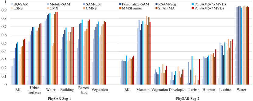
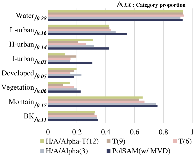
Additionally, the metrics for each category of the two datasets are visualized in Fig. 9, providing a clear comparison of the results. The blue bars represent our PolSAM(w/o MVD) method, corresponding to the blue-themed SAM-based approaches, while the red bars indicate our PolSAM(w/ MVD) method, aligned with the red-themed multimodal methods. Our methods demonstrate three key strengths. First, both PolSAM (w/ MVD) and PolSAM (w/o MVD) consistently outperform other methods across most categories. Second, PolSAM (w/ MVD) generally delivers better overall performance than PolSAM (w/o MVD), highlighting the advantage of incorporating MVD. Finally, for the PhySAR-Seg-1 dataset, our method achieves the best results across nearly every category. For the PhySAR-Seg-2 dataset, particularly in the urban class where double-bounce scattering is dominant but the class proportion is small, our method demonstrates significant improvements compared to other approaches. This indicates that, even in challenging scenarios, effectively leveraging MVD information can substantially enhance segmentation accuracy.
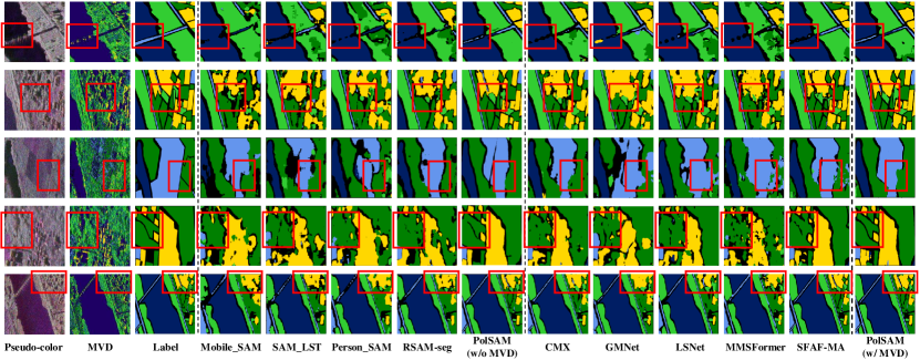
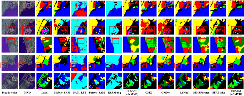
Visualization. Fig. 10 showcases the visualization of segmentation outcomes for the PhySAR-Seg-1 dataset, comparing SAM-based and multimodal fusion-based methods. Similarly, Fig. 11 presents the segmentation result visualizations for the PhySAR-Seg-2 dataset. It can be seen that PolSAM has obtained the most refined segmentation results among those methods. Note that the MVD image provides distinct physical properties of terrain, which depict high-level semantic information better than pseudo-colored images. On the contrary, the pseudo-colored image contains richer texture information than MVD. The multi-input complementarities in feature and semantic level are clearly reflected. The proposed PolSAM can explicitly leverage the semantic information with the fusion prompt, which is used to hint the decoder for better segmentation.
Through a comparison of the red-boxed details in the figure, PolSAM demonstrates a strong capability in capturing edge information between different terrain classes in segmentation results. LSNet [55], which incorporates edge constraints to preserve boundary information during training, outperforms several comparative methods that do not utilize such constraints. However, given the inherent limitations of PolSAR data, including speckle noise and indistinct edges in certain terrain classes, its results remain somewhat unsatisfactory. In contrast, our method achieves better results by more effectively leveraging semantic information to guide the segmentation process, leading to clearer edges and improved overall accuracy.
| Data | Encoder | Decoder | PhySAR-Seg-1(%) | PhySAR-Seg-2(%) | ||||||||
|---|---|---|---|---|---|---|---|---|---|---|---|---|
| MVD | Adapter | FFP | SFP-1 | SFP-2 | mAcc | mF1 score | mIoU | mAcc | mF1 score | mIoU | ||
| Baseline | ✗ | ✗ | ✗ | ✗ | ✗ | ✗ | 70.83 | 71.42 | 56.49 | 63.48 | 43.29 | 32.05 |
| M1 | \usym1F5F8 | ✗ | ✗ | \usym1F5F8 | \usym1F5F8 | \usym1F5F8 | 72.83 | 73.96 | 59.55 | 70.77 | 55.38 | 41.00 |
| M2 | \usym1F5F8 | ✗ | \usym1F5F8 | \usym1F5F8 | \usym1F5F8 | \usym1F5F8 | 75.41 | 76.51 | 62.76 | 74.63 | 57.21 | 43.20 |
| M3 | \usym1F5F8 | \usym1F5F8 | ✗ | \usym1F5F8 | \usym1F5F8 | \usym1F5F8 | 82.37 | 83.44 | 71.33 | 74.94 | 59.78 | 45.38 |
| M4 | \usym1F5F8 | \usym1F5F8 | \usym1F5F8 | ✗ | ✗ | ✗ | 80.64 | 81.71 | 69.58 | 72.26 | 53.38 | 40.62 |
| M5 | \usym1F5F8 | \usym1F5F8 | \usym1F5F8 | \usym1F5F8 | \usym1F5F8 | ✗ | 81.24 | 82.30 | 70.10 | 73.17 | 57.77 | 41.61 |
| PolSAM(w/o MVD) | ✗ | \usym1F5F8 | \usym1F5F8 | \usym1F5F8 | \usym1F5F8 | \usym1F5F8 | 82.62 | 83.37 | 71.84 | 73.69 | 59.69 | 45.30 |
| PolSAM(w/ MVD) | \usym1F5F8 | \usym1F5F8 | \usym1F5F8 | \usym1F5F8 | \usym1F5F8 | \usym1F5F8 | 83.70 | 84.71 | 73.55 | 76.47 | 61.40 | 46.55 |
V-C Ablation Studies on Module Design
We perform comprehensive module ablation studies on both datasets to assess the efficacy of the modules. As shown in Table III, we first define the baseline model as the original SAM that takes the pseudo-colored SAR image as the input and only train the mask decoder part. The following models, M1 to M5, all take two inputs. Compared to our method PolSAM (w/ MVD), M2, M3, and M1 are designed to validate the effectiveness of the adapter, FFP, and their combined impact, respectively. It can be seen that the adapter in the PolSAM encoder has a significant influence of the model performance, and the proposed FFP can also improve the result to a certain extent. The effectiveness of the proposed progressive SFP can be verified by comparing the performance of M4. The implementation of the SFP module enhances the overall performance of the model, as evidenced by the results. Compared to M4, our method enhances performance by 3.97% on the PhySAR-Seg-1 dataset, while on the PhySAR-Seg-2 dataset, the enhancement is 5.93%.
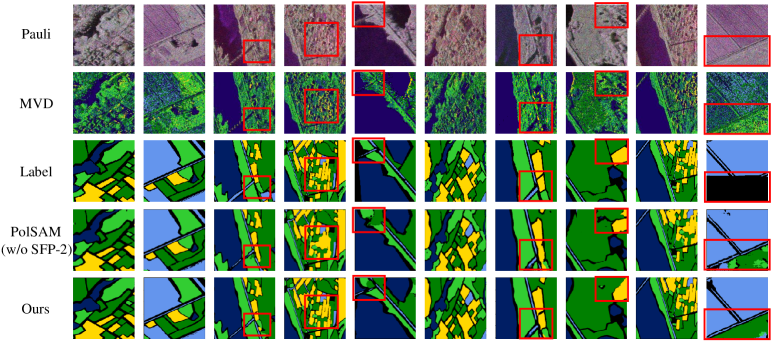
To validate the effectiveness of the progressive design of the SFP module, we conducted an additional ablation study on SFP-2, referred to as M5. The visualization results on the PhySAR-Seg-1 dataset are presented in Fig. 12. Our method, PolSAM (w/ MVD), which integrates SFP-2, significantly outperforms the version without SFP-2, especially in the details highlighted by the red box. It is important to note that the labels in the last column of images are incomplete; however, our results still accurately predict the same semantic categories as the original images. This indicates that the progressive design effectively enhances the interaction between multi-input features and high-level semantic features, enriching the semantic information embedded in the fusion prompt.
To further demonstrate the validity of our proposed method, we conducted an ablation study on the MVD. In the PolSAM (w/o MVD) experiment, we replaced the MVD with pseudo-colored images. Despite this modification, PolSAM (w/o MVD) still shows significant improvements over the baseline, achieving mIoU increases of 15.35% on the PhySAR-Seg-1 dataset and 8.64% on the PhySAR-Seg-2 dataset, illustrating the soundness of our overall model design. However, when compared to PolSAM (w/ MVD), PolSAM (w/o MVD) falls short. PolSAM (w/ MVD) achieves even greater mIoU increases of 17.06% on PhySAR-Seg-1 and 9.89% on PhySAR-Seg-2 compared to the baseline, highlighting that the MVD, representing the scattering mechanism, provides valuable multidimensional information that enhances segmentation performance, particularly in capturing details.
V-D Discussions on Semantic prompt
The Effectiveness of Semantic Prompts. To verify the effectiveness of the proposed SFP, we analyze the learned ultimate sparse and dense prompt embeddings at the semantic level on the PhySAR-Seg-1 dataset, namely and , where denotes the number of sparse prompts. These embeddings reflect semantic prompts associated with class information and mask information, respectively. To better illustrate the semantic prompt, the dense prompt embedding is averaged along the channel dimension, yielding for visualization. As shown in the second row of Fig. 13(a), clearly highlights the semantic map corresponding to the annotated mask. Additionally, we multiply the sparse prompt embedding by the dense prompt embedding and average along the channel dimension to obtain the class-aware dense prompt visualization map . Notably, the class-aware prompt reveals more discriminative semantics, as illustrated in the third row of Fig. 13(a).
In our experiments, the number of sparse prompt is set to the number of semantic class. Consequently, we visualize class-specific fusion prompt maps denoted as in Fig. 13(b) for discussion. It can be observed that the class-specific fusion prompt map shows significant correlation with each class. The results illustrate the explicit semantic meanings of the learned fusion prompt, which play an important role to guide the decoder to learn the segmentation result.
| No. of SP | mAcc | mF1 score | mIoU |
|---|---|---|---|
| 3 | 83.40 | 84.07 | 72.68 |
| 6(classes) | 83.70 | 84.71 | 73.55 |
| 2 * 6 | 82.34 | 83.12 | 71.42 |
| 4 * 6 | 83.43 | 84.29 | 73.01 |
| 10 * 6 | 83.07 | 83.78 | 72.25 |
| 20 * 6 | 83.37 | 84.28 | 73.06 |
Sparse Prompt Parameter Selection. Note that the number of sparse prompts reflects the degree of semantic correlation. Consequently, we conducted ablation experiments to analyze its impact on model performance. As shown in Table IV, we explored six different values of , each being a multiple of the number of categories in the dataset. This experiment was performed on the PhySAR-Seg-1 dataset, where the model achieved the best performance when , which matches the number of classes. However, when was increased significantly to 10 or 20 times the number of categories, the network’s parameter count grew, but the performance metrics did not consistently improve. This indicates that an excessively large leads to parameter redundancy, while a value of smaller than the number of classes can cause semantic confusion. Therefore, we infer that the sparse prompt is closely linked to semantic information, enabling the semantic-level fusion prompt to align semantically during training, which ultimately enhances segmentation results.
| Metrics | Inputs: H/A/Alpha()[56] T[57] | |||||
|---|---|---|---|---|---|---|
| (%) | None | H/A/ | T(6) | T(9) | H/A/_T | MVD |
| BK | 29.53 | 33.93 | 33.74 | 32.20 | 32.68 | 34.83 |
| Montain | 64.25 | 74.96 | 66.87 | 63.28 | 65.59 | 75.88 |
| Vegetation | 13.23 | 19.90 | 17.81 | 10.34 | 15.02 | 22.63 |
| Developed | 9.21 | 23.12 | 15.48 | 18.21 | 19.73 | 18.13 |
| I-urban | 0.01 | 15.12 | 15.57 | 19.66 | 11.93 | 30.76 |
| H-urban | 18.98 | 31.68 | 26.21 | 20.56 | 31.30 | 42.43 |
| L-urban | 30.65 | 46.83 | 43.43 | 42.59 | 42.36 | 54.57 |
| Water | 90.51 | 91.81 | 94.15 | 93.55 | 93.74 | 93.31 |
| \hdashlinemAcc | 63.48 | 72.81 | 69.29 | 65.11 | 69.51 | 76.47 |
| mF1 score | 43.29 | 57.34 | 56.02 | 51.59 | 52.82 | 61.40 |
| mIoU | 32.05 | 42.25 | 39.14 | 37.53 | 39.05 | 46.55 |
| \hdashlineFPS | 26.63 | 22.42 | 12.81 | 7.20 | 5.68 | 18.74 |
| Memory(GB) | - | 6.49 | 12.99 | 19.46 | 25.9 | 0.049 |
V-E Discussions on Effectiveness of MVD.
Utilizing MVD offers two notable benefits. Initially, the complex information is transformed into a compact format through a series of processing stages. This process allows the data to visually represent the scattering mechanism, effectively conveying the physical information in a way that is intuitively understandable for humans, while also being highly correlated with semantic information. Additionally, MVD requires only a small amount of memory, significantly reducing the storage needed for complex data and improving efficiency in data loading and preprocessing for neural networks.
To validate the effectiveness of MVD, we conducted experiments comparing different polarimetric decomposition features as substitutes for MVD in the PolSAM. The results, shown in Table V, evaluate the performance of four feature combinations, primarily based on the H/A/Alpha decomposition method [56] and the polarization coherence matrix (). We compared the performance metrics, frame per second (FPS), and data memory usage against these alternative decomposition methods.
The H/A/Alpha decomposition method [56] is used to analyse scattering mechanisms in PolSAR data. The entropy (H) and alpha angle () are calculated using the eigenvalues and eigenvectors of the coherency matrix. This allows for the characterisation of surface, double-bounce, and volume. The entropy (H) is calculated using the formula [], where represents the probabilities associated with the eigenvalues. The alpha angle () is calculated using the formula [], where represents the corresponding scattering mechanism angles. This technique offers the benefit of offering a comprehensive explanation of scattering mechanisms, but it may be restricted by its susceptibility to noise and the assumption of simplistic scattering models, which may not accurately represent more complex ground features.
The polarization coherence matrix is derived from the Pauli scattering vector under the reciprocity condition and represents the fully polarimetric information in PolSAR imaging [57]. The matrix is given by:
where is the Pauli scattering vector and is its conjugate transpose. The elements are the entries (i, j) of the matrix , and denotes the rescattered return of the horizontal transmitting and vertical receiving polarizations. The polarization coherence matrix is a symmetric matrix, meaning its upper triangular elements can fully represent its polarimetric features. As a result, the decomposition of yields nine components: , , and (the diagonal elements representing the power in each polarization channel), , (the real and imaginary parts of the cross-polarization components), , (additional cross-polarization components), and , (remaining cross-polarization components).
The real parts of these upper triangular elements form the six-channel T(6) dataset, as shown in the third column of Table V. The full set of real and imaginary components together constitute the nine-channel T(9) dataset, represented in the fourth column. Additionally, the H/A/Alpha_T(12) approach in the fifth column combines the three channels from the H/A/Alpha decomposition with the nine-channel data from the decomposition, resulting in a comprehensive twelve-channel dataset.
The comparison results in the table first demonstrate the effectiveness of the PolSAM architecture, as all four methods incorporating different polarimetric information show improvements over the baseline, confirming the validity of the model. Furthermore, when comparing these methods to our approach using MVD, the advantages of incorporating MVD become even more evident. Our MVD approach, compared to the second-best method, H/A/Alpha decomposition, shows clear improvements in evaluation metrics, with increases of 3.66% in mAcc, 4.06% in mean F1 score, and 4.3% in mIoU. These results clearly demonstrate that integrating MVD further enhances segmentation performance, highlighting the added value it brings to the PolSAM architecture.
To further evaluate the effectiveness of our method, we conducted a detailed analysis of IoU metrics for each class in the PhySAR-Seg-2 dataset. The results, presented in Table V and visualized in Fig. 14, show that our method using MVD achieves the best results across most classes, particularly for the urban class, which is characterized by double-bounce scattering and has the lowest overall proportion in the dataset.
For loading a batch of 668 image pairs, our method reduces the loading time by 16.52 seconds, 57.11 seconds, and 82.07 seconds compared to the T(6), T(9), and H/A/Alpha_T(12) approaches, respectively. In terms of data storage, MVD occupies only 49 MB of memory, representing just 0.755%, 0.377%, 0.252%, and 0.189% of the capacity utilized by the other four methods. These results highlight the clear advantages of MVD, making it a highly efficient and effective option for polarimetric data processing.
VI Conclusion
In this study, we proposed PolSAM, a novel segmentation framework designed for PolSAR image analysis. PolSAM utilizes the Microwave Vision Data (MVD) representation, which encodes scattering characteristics into a lightweight and interpretable format, offering both visual and physical insights. By integrating features from pseudo-colored SAR images and MVD, PolSAM effectively combines complementary information to guide the segmentation process. The framework incorporates a FFP module for the initial integration of features, supported by an adapter to align representation spaces and address feature differences. Additionally, the SFP module refines segmentation through multi-level feature interactions, enabling the effective incorporation of semantic and physical scattering characteristics. Together, these components enable PolSAM to achieve efficient and accurate segmentation while maintaining high interpretability.
In the future, we aim to explore more robust methods to enhance the adaptability of large models to SAR data for improved utilization efficiency. Additionally, considering the rich physical scattering characteristics inherent in PolSAR data, we will investigate approaches to further enhance segmentation results for PolSAR images.
References
- [1] Z. Tirandaz, G. Akbarizadeh, and H. Kaabi, “Polsar image segmentation based on feature extraction and data compression using weighted neighborhood filter bank and hidden markov random field-expectation maximization,” Measurement, vol. 153, p. 107432, 2020.
- [2] Z. Wang, X. Zeng, Z. Yan, J. Kang, and X. Sun, “Air-polsar-seg: A large-scale data set for terrain segmentation in complex-scene polsar images,” IEEE J. Sel. Top. Appl. Earth Observ. Remote Sens., vol. 15, pp. 3830–3841, 2022.
- [3] X. Liu, L. Jiao, X. Tang, Q. Sun, and D. Zhang, “Polarimetric convolutional network for polsar image classification,” IEEE Trans. Geosci. Remote Sens., vol. 57, no. 5, pp. 3040–3054, 2018.
- [4] L. Zhang, S. Zhang, B. Zou, and H. Dong, “Unsupervised deep representation learning and few-shot classification of polsar images,” IEEE Trans. Geosci. Remote Sens., vol. 60, pp. 1–16, 2020.
- [5] R. Qin, X. Fu, and P. Lang, “Polsar image classification based on low-frequency and contour subbands-driven polarimetric senet,” IEEE J. Sel. Top. Appl. Earth Observ. Remote Sens., vol. 13, pp. 4760–4773, 2020.
- [6] M. Ghanbari, L. Xu, and D. A. Clausi, “Local and global spatial information for land cover semisupervised classification of complex polarimetric sar data,” IEEE J. Sel. Top. Appl. Earth Observ. Remote Sens., vol. 16, pp. 3892–3904, 2023.
- [7] L. Li, L. Ma, L. Jiao, F. Liu, Q. Sun, and J. Zhao, “Complex contourlet-cnn for polarimetric sar image classification,” Pattern Recognition, vol. 100, p. 107110, 2020.
- [8] O. Antropov, Y. Rauste, H. Astola, J. Praks, T. Häme, and M. T. Hallikainen, “Land cover and soil type mapping from spaceborne polsar data at l-band with probabilistic neural network,” IEEE Trans. Geosci. Remote Sens., vol. 52, no. 9, pp. 5256–5270, 2013.
- [9] H. Shen, L. Lin, J. Li, Q. Yuan, and L. Zhao, “A residual convolutional neural network for polarimetric sar image super-resolution,” ISPRS J. Photogramm. Remote Sens., vol. 161, pp. 90–108, 2020.
- [10] X. Pu, H. Jia, L. Zheng, F. Wang, and F. Xu, “Classwise-sam-adapter: Parameter efficient fine-tuning adapts segment anything to sar domain for semantic segmentation,” arXiv preprint arXiv:2401.02326, 2024.
- [11] L. Yu, Z. Zeng, A. Liu, X. Xie, H. Wang, F. Xu, and W. Hong, “A lightweight complex-valued deeplabv3+ for semantic segmentation of polsar image,” IEEE J. Sel. Top. Appl. Earth Observ. Remote Sens., vol. 15, pp. 930–943, 2022.
- [12] Z. Kuang, H. Bi, F. Li, C. Xu, and J. Sun, “Polarimetry-inspired contrastive learning for class-imbalanced polsar image classification,” IEEE Trans. Geosci. Remote Sens., 2024.
- [13] W. Hua, Q. Hou, X. Jin, L. Liu, N. Sun, and Z. Meng, “A feature fusion network for polsar image classification based on physical features and deep features,” IEEE Geosci. Remote Sens. Lett., 2024.
- [14] H. Dong, L. Zhang, and B. Zou, “Exploring vision transformers for polarimetric sar image classification,” IEEE Trans. Geosci. Remote Sens., vol. 60, pp. 1–15, 2021.
- [15] A. Jamali, S. K. Roy, A. Bhattacharya, and P. Ghamisi, “Local window attention transformer for polarimetric sar image classification,” IEEE Geosci. Remote Sens. Lett., vol. 20, pp. 1–5, 2023.
- [16] W. Wu, H. Li, X. Li, H. Guo, and L. Zhang, “Polsar image semantic segmentation based on deep transfer learning—realizing smooth classification with small training sets,” IEEE Geosci. Remote Sens. Lett., vol. 16, no. 6, pp. 977–981, 2019.
- [17] Z. Fang, G. Zhang, Q. Dai, B. Xue, and P. Wang, “Hybrid attention-based encoder–decoder fully convolutional network for polsar image classification,” Remote Sens., vol. 15, no. 2, p. 526, 2023.
- [18] X. Zeng, Z. Wang, K. Feng, X. Gao, and X. Sun, “Ts-shes: Terrain segmentation in complex-valued polsar images via scattering harmonization and explicit supervision,” IEEE Trans. Geosci. Remote Sens., vol. 60, pp. 1–20, 2022.
- [19] X. Zeng, Z. Wang, Y. Wang, X. Rong, P. Guo, X. Gao, and X. Sun, “Semipscn: Polarization semantic constraint network for semi-supervised segmentation in large-scale and complex-valued polsar images,” IEEE Trans. Geosci. Remote Sens., 2023.
- [20] Z. Huang, X. Yao, Y. Liu, C. O. Dumitru, M. Datcu, and J. Han, “Physically explainable cnn for sar image classification,” ISPRS J. Photogramm. Remote Sens., vol. 190, pp. 25–37, 2022.
- [21] A. Kirillov, E. Mintun, N. Ravi, H. Mao, C. Rolland, L. Gustafson, T. Xiao, S. Whitehead, A. C. Berg, W.-Y. Lo et al., “Segment anything,” in Int. Conf. Comput. Vis., 2023, pp. 4015–4026.
- [22] J. Sun, S. Yang, X. Gao, D. Ou, Z. Tian, J. Wu, and M. Wang, “Masa-segnet: A semantic segmentation network for polsar images,” Remote Sens., vol. 15, no. 14, p. 3662, 2023.
- [23] G. Gao, Q. Bai, C. Zhang, L. Zhang, and L. Yao, “Dualistic cascade convolutional neural network dedicated to fully polsar image ship detection,” ISPRS J. Photogramm. Remote Sens., vol. 202, pp. 663–681, 2023.
- [24] Q. Zhang, C. He, B. He, and M. Tong, “Learning scattering similarity and texture-based attention with convolutional neural networks for polsar image classification,” IEEE Trans. Geosci. Remote Sens., vol. 61, pp. 1–19, 2023.
- [25] D. Xiang, H. Ding, X. Sun, J. Cheng, C. Hu, and Y. Su, “Polsar image registration combining siamese multiscale attention network and joint filter,” IEEE Trans. Geosci. Remote Sens., 2024.
- [26] D. Xiao, Z. Wang, Y. Wu, X. Gao, and X. Sun, “Terrain segmentation in polarimetric sar images using dual-attention fusion network,” IEEE Geosci. Remote Sens. Lett., vol. 19, pp. 1–5, 2020.
- [27] J. Shi, T. He, S. Ji, M. Nie, and H. Jin, “Cnn-improved superpixel-to-pixel fuzzy graph convolution network for polsar image classification,” IEEE Trans. Geosci. Remote Sens., 2023.
- [28] J. Ge, H. Zhang, L. Xu, C. Sun, H. Duan, Z. Guo, and C. Wang, “A physically interpretable rice field extraction model for polsar imagery,” Remote Sens., vol. 15, no. 4, p. 974, 2023.
- [29] S. Hochstuhl, N. Pfeffer, A. Thiele, H. Hammer, and S. Hinz, “Your input matters—comparing real-valued polsar data representations for cnn-based segmentation,” Remote Sens., vol. 15, no. 24, p. 5738, 2023.
- [30] J. Geng, R. Wang, and W. Jiang, “Polarimetric sar image classification based on feature enhanced superpixel hypergraph neural network,” IEEE Trans. Geosci. Remote Sens., vol. 60, pp. 1–12, 2022.
- [31] R. Wang, Y. Nie, and J. Geng, “Multiscale superpixel-guided weighted graph convolutional network for polarimetric sar image classification,” IEEE J. Sel. Top. Appl. Earth Observ. Remote Sens., 2024.
- [32] R. Zhang, Z. Jiang, Z. Guo, S. Yan, J. Pan, X. Ma, H. Dong, P. Gao, and H. Li, “Personalize segment anything model with one shot,” arXiv preprint arXiv:2305.03048, 2023.
- [33] C. Zhang, D. Han, Y. Qiao, J. U. Kim, S.-H. Bae, S. Lee, and C. S. Hong, “Faster segment anything: Towards lightweight sam for mobile applications,” arXiv preprint arXiv:2306.14289, 2023.
- [34] J. Wu, R. Fu, H. Fang, Y. Liu, Z. Wang, Y. Xu, Y. Jin, and T. Arbel, “Medical sam adapter: Adapting segment anything model for medical image segmentation,” arXiv preprint arXiv:2304.12620, 2023.
- [35] S. Chai, R. K. Jain, S. Teng, J. Liu, Y. Li, T. Tateyama, and Y.-w. Chen, “Ladder fine-tuning approach for sam integrating complementary network,” arXiv preprint arXiv:2306.12737, 2023.
- [36] L. Ke, M. Ye, M. Danelljan, Y.-W. Tai, C.-K. Tang, F. Yu et al., “Segment anything in high quality,” Adv. Neural Inform. Process. Syst., vol. 36, 2024.
- [37] W. Yue, J. Zhang, K. Hu, Q. Wu, Z. Ge, Y. Xia, J. Luo, and Z. Wang, “Part to whole: Collaborative prompting for surgical instrument segmentation,” arXiv preprint arXiv:2312.14481, 2023.
- [38] W. Yue, J. Zhang, K. Hu, Y. Xia, J. Luo, and Z. Wang, “Surgicalsam: Efficient class promptable surgical instrument segmentation,” in AAAI Conf. Art. Intell., vol. 38, 2024, pp. 6890–6898.
- [39] Q. Xu, J. Li, X. He, Z. Liu, Z. Chen, W. Duan, C. Li, M. M. He, F. B. Tesema, W. P. Cheah et al., “Esp-medsam: Efficient self-prompting sam for universal domain-generalized medical image segmentation,” arXiv preprint arXiv:2407.14153, 2024.
- [40] K. Chen, C. Liu, H. Chen, H. Zhang, W. Li, Z. Zou, and Z. Shi, “Rsprompter: Learning to prompt for remote sensing instance segmentation based on visual foundation model,” IEEE Trans. Geosci. Remote Sens., 2024.
- [41] J. Zhang, X. Yang, R. Jiang, W. Shao, and L. Zhang, “Rsam-seg: A sam-based approach with prior knowledge integration for remote sensing image semantic segmentation,” arXiv preprint arXiv:2402.19004, 2024.
- [42] Z. Yan, J. Li, X. Li, R. Zhou, W. Zhang, Y. Feng, W. Diao, K. Fu, and X. Sun, “Ringmo-sam: A foundation model for segment anything in multimodal remote-sensing images,” IEEE Trans. Geosci. Remote Sens., vol. 61, pp. 1–16, 2023.
- [43] L. Zheng, X. Pu, and F. Xu, “Tuning a sam-based model with multi-cognitive visual adapter to remote sensing instance segmentation,” arXiv preprint arXiv:2408.08576, 2024.
- [44] Y. Zhang, T. Cheng, R. Hu, H. Liu, L. Ran, X. Chen, W. Liu, X. Wang et al., “Evf-sam: Early vision-language fusion for text-prompted segment anything model,” arXiv preprint arXiv:2406.20076, 2024.
- [45] Z. Xie, B. Guan, W. Jiang, M. Yi, Y. Ding, H. Lu, and L. Zhang, “Pa-sam: Prompt adapter sam for high-quality image segmentation,” arXiv preprint arXiv:2401.13051, 2024.
- [46] Z. Huang, M. Datcu, Z. Pan, X. Qiu, and B. Lei, “Hdec-tfa: An unsupervised learning approach for discovering physical scattering properties of single-polarized sar image,” IEEE Trans. Geosci. Remote Sens., vol. 59, no. 4, pp. 3054–3071, 2021.
- [47] D. Ratha, A. Bhattacharya, and A. C. Frery, “Unsupervised classification of polsar data using a scattering similarity measure derived from a geodesic distance,” IEEE Geosci. Remote Sens. Lett., vol. 15, no. 1, pp. 151–155, 2017.
- [48] J. Yan, Q. Xiaolan, P. Jie, S. Songtao, W. Zezhong, W. Wei, and Y. Hong, “Mpolsar-1.0: Multidimensional sar multiband fully polarized fine classification dataset,” 雷达学报, vol. 13, no. 3, pp. 525–538, 2024.
- [49] Gaofen-3, “Gaofen-3 (gf3) full (quad) polarimetric sample datasets,” 2019, accessed: Feb. 3, 2019. [Online]. Available: https://www.ietr.fr/GF3/
- [50] M. Jia, L. Tang, B.-C. Chen, C. Cardie, S. Belongie, B. Hariharan, and S.-N. Lim, “Visual prompt tuning,” in Eur. Conf. Comput. Vis. Springer, 2022, pp. 709–727.
- [51] M. K. Reza, A. Prater-Bennette, and M. S. Asif, “Mmsformer: Multimodal transformer for material and semantic segmentation,” IEEE Open J. Signal Process., 2024.
- [52] X. He, M. Wang, T. Liu, L. Zhao, and Y. Yue, “Sfaf-ma: Spatial feature aggregation and fusion with modality adaptation for rgb-thermal semantic segmentation,” IEEE Trans. Instrum. Meas., 2023.
- [53] W. Zhou, J. Liu, J. Lei, L. Yu, and J.-N. Hwang, “Gmnet: Graded-feature multilabel-learning network for rgb-thermal urban scene semantic segmentation,” IEEE Trans. Image Process., vol. 30, pp. 7790–7802, 2021.
- [54] J. Zhang, H. Liu, K. Yang, X. Hu, R. Liu, and R. Stiefelhagen, “Cmx: Cross-modal fusion for rgb-x semantic segmentation with transformers,” IEEE Trans. Intell. Transp. Syst., 2023.
- [55] W. Zhou, Y. Zhu, J. Lei, R. Yang, and L. Yu, “Lsnet: Lightweight spatial boosting network for detecting salient objects in rgb-thermal images,” IEEE Trans. Image Process., vol. 32, pp. 1329–1340, 2023.
- [56] S. R. Cloude and E. Pottier, “An entropy based classification scheme for land applications of polarimetric sar,” IEEE Trans. Geosci. Remote Sens., vol. 35, no. 1, pp. 68–78, 1997.
- [57] S.-W. Chen and C.-S. Tao, “Polsar image classification using polarimetric-feature-driven deep convolutional neural network,” IEEE Geosci. Remote Sens. Lett., vol. 15, no. 4, pp. 627–631, 2018.
![[Uncaptioned image]](/html/2412.12737/assets/x15.png) |
Yuqing Wang is currently working toward the Ph.D. degree in the School of Automation, Northwestern Polytechnical University, Xi’an, China. Her research interests include computer vision, synthetic aperture radar (SAR) image interpretation, and multimodal image fusion. |
![[Uncaptioned image]](/html/2412.12737/assets/x16.png) |
Zhongling Huang (huangzhongling@nwpu.edu.cn) received her B.Sc. degree in electronic information science and technology from Beijing Normal University, Beijing, China, in 2015, and her Ph.D. degree from the University of Chinese Academy of Sciences (UCAS) and the Aerospace Information Research Institute, Chinese Academy of Sciences, Beijing, China, in 2020. She served as a visiting scholar in the German Aerospace Center during 2018–2019, funded by UCAS. She is currently working in the Brain and Artificial Intelligence Lab, School of Automation, Northwestern Polytechnical University, Xi’an 710072, China. Her research interests include explainable deep learning for synthetic aperture radar (SAR), SAR image interpretation, deep learning, and remote sensing data mining. |
![[Uncaptioned image]](/html/2412.12737/assets/x17.png) |
Shuxin Yang is currently a master’s student at Northwestern Polytechnical University in Xi’an, Shanxi. His research direction is SAR image target detection in computer vision. |
![[Uncaptioned image]](/html/2412.12737/assets/x18.png) |
Hao Tang is an Assistant Professor at Peking University, China. Previously, he held postdoctoral positions at both CMU, USA, and ETH Zürich, Switzerland. He earned a master’s degree from Peking University, China, and a Ph.D. from the University of Trento, Italy. He was a visiting Ph.D. student at the University of Oxford, UK, and an intern at IIAI, UAE. His research interests include AIGC, AI4Science, machine learning, computer vision, embodied AI, and their applications to scientific domains. |
![[Uncaptioned image]](/html/2412.12737/assets/x19.png) |
Xiaolan Qiu (Senior Member, IEEE) received the B.S. degree in electronic engineering and information science from the University of Science and Technology of China, Hefei, China, in 2004, and the Ph.D. degree in signal and information processing from the Graduate University of Chinese Academy of Sciences, Beijing, China, in 2009. She is with the National Key Laboratory of Microwave Imaging Technology, Chinese Academy of Sciences, Beijing 100090, China, and also with the Aerospace Information Research Institute, Chinese Academy of Sciences, Beijing 100094, China. Her research interests include synthetic aperture radar (SAR) imaging, SAR simulation, and SAR 3-D reconstruction. |
![[Uncaptioned image]](/html/2412.12737/assets/x20.png) |
Junwei Han (Fellow, IEEE) is currently a Professor in the School of Automation, Northwestern Polytechnical University. His research interests include computer vision, pattern recognition, remote sensing image analysis, and brain imaging analysis. He has published more than 70 papers in top journals such as IEEE TPAMI, TNNLS, IJCV, and more than 30 papers in top conferences such as CVPR, ICCV, MICCAI, and IJCAI. He is an Associate Editor for several journals such as IEEE TNNLS and IEEE TMM. |
![[Uncaptioned image]](/html/2412.12737/assets/x21.png) |
Dingwen Zhang (Member, IEEE) received the Ph.D. degree from Northwestern Polytechnical University, Xi’an, China, in 2018. He is a Professor with the School of Automation, Northwestern Polytechnical University. From 2015 to 2017, he was a Visiting Scholar with the Robotic Institute, Carnegie Mellon University, Pittsburgh, PA, USA. His research interests include computer vision and multimedia processing, especially on saliency detection and weakly supervised learning. |