Runtime Analysis for Multi-Objective Evolutionary Algorithms in Unbounded Integer Spaces
Abstract
Randomized search heuristics have been applied successfully to a plethora of problems. This success is complemented by a large body of theoretical results. Unfortunately, the vast majority of these results regard problems with binary or continuous decision variables – the theoretical analysis of randomized search heuristics for unbounded integer domains is almost nonexistent. To resolve this shortcoming, we start the runtime analysis of multi-objective evolutionary algorithms, which are among the most successful randomized search heuristics, for unbounded integer search spaces. We analyze single- and full-dimensional mutation operators with three different mutation strengths, namely changes by plus/minus one (unit strength), random changes following a law with exponential tails, and random changes following a power-law. The performance guarantees we prove on a recently proposed natural benchmark problem suggest that unit mutation strengths can be slow when the initial solutions are far from the Pareto front. When setting the expected change right (depending on the benchmark parameter and the distance of the initial solutions), the mutation strength with exponential tails yields the best runtime guarantees in our results – however, with a wrong choice of this expectation, the performance guarantees quickly become highly uninteresting. With power-law mutation, which is an essentially parameter-less mutation operator, we obtain good results uniformly over all problem parameters and starting points. We complement our mathematical findings with experimental results that suggest that our bounds are not always tight. Most prominently, our experiments indicate that power-law mutation outperforms the one with exponential tails even when the latter uses a near-optimal parametrization. Hence, we suggest to favor power-law mutation for unknown problems in integer spaces.
Introduction
For more than thirty years, the mathematical runtime analysis of randomized search heuristics has supported the design and analysis of these important algorithms, both in single- and in multi-objective optimization (Neumann and Witt 2010; Auger and Doerr 2011; Jansen 2013; Zhou, Yu, and Qian 2019; Doerr and Neumann 2020). While in practice heuristics are successfully employed for all types of decision variables, the mathematical analysis is mostly concentrated on binary or continuous variables. Discrete spaces with more than two variable values are considered far more infrequently. Theoretical works include runtime analyses for evolutionary algorithms, ant-colony optimizers, and estimation-of-distribution algorithms on categorical variables, e.g., Scharnow, Tinnefeld, and Wegener (2004); Baswana et al. (2009); Sudholt and Thyssen (2012); Doerr, Happ, and Klein (2012); Ben Jedidia, Doerr, and Krejca (2024); Adak and Witt (2024). The theoretical research for cardinal variables was started by Doerr, Johannsen, and Schmidt (2011); Doerr and Pohl (2012); Kötzing, Lissovoi, and Witt (2015) with analyses how the EA optimizes multi-valued linear functions. Doerr, Doerr, and Kötzing (2018, 2019) showed that for multi-valued variables larger mutation rates can be advantageous. Submodular functions with multi-valued discrete domain were studied by Qian et al. (2018a, b). We are only aware of two analyses for search spaces consisting of unbounded integer variables. The first is (Rudolph 2023), which is a single-objective analysis of subproblems of a multi-objective problem. The second is (Harder et al. 2024), which considers a single-objective problem and shows the benefit of larger mutation rates. We are not aware of any true multi-objective works with multi-valued variables, despite considerable recent theoretical research on multi-objective heuristics (Zheng, Liu, and Doerr 2022; Dang et al. 2023; Cerf et al. 2023; Do et al. 2023; Dinot et al. 2023; Zheng and Doerr 2024; Zheng et al. 2024; Bian et al. 2024; Ren et al. 2024).
Since multi-objective optimization is an area where heuristics, in particular, evolutionary algorithms, are intensively used and with great success (see, e.g., the famous NSGA-II algorithm (Deb et al. 2002) with more than citations on Google Scholar), we start in this work the mathematical runtime analysis for truly multi-objective optimization problems in unbounded integer search spaces. For the benchmark problems proposed by Rudolph (2023), we analyze the performance of the simple evolutionary multi-objective optimizer (SEMO) (Laumanns et al. 2002) and the Global SEMO (GSEMO) (Giel 2003), the two most prominent evolutionary algorithms in the runtime analysis of multi-objective evolutionary algorithms. Our objective is to understand, via theoretical means, what are suitable mutation operators for unbounded integer domains. We propose three natural operators, changing variables (i) by plus or minus one (unit mutation strength), (ii) by a random value drawn from a symmetric distribution with exponential tails, and (iii) by a random value drawn from a symmetric power-law distribution.
We conduct an extensive mathematical runtime analysis for these two algorithms with the three mutation operators (with general parameters, where applicable) on the benchmark with general width parameter of the Pareto front for a general initial solution . Our results, presented in more detail later in this work when all ingredients are made precise, indicate the following. All algorithm variants can compute the full Pareto front of our benchmark problem in reasonable time. The unit mutation strength, not surprisingly can lead to a slow progress towards the Pareto front when the initial solution is far, but it also results in a slow exploration of the Pareto front after having reached it. The performance with the exponential-tail mutation strength depends heavily on the variance parameter (which is essentially the reciprocal of the expected absolute change). With an optimal choice of , depending on the benchmark parameter and the starting solution , this operator leads to the best performance guarantee among our results. However, our runtime guarantees strongly depend on the relation of , , and ; hence a suboptimal choice of can quickly lead to very weak performance guarantees. The power-law mutation strength is a good one-size-fits-all solution. Being an essentially parameter-less operator, it achieves a good performance uniformly over all values of and , clearly beating the unit mutation strength for larger instances or distances of the starting solution from the Pareto front.
We complement our theoretical results by an empirical analysis, aimed to understand how tight our guarantees are. We observe that the best-possible parameter regime for the exponential-tail mutation is within the range of our mathematical findings. However, surprisingly, the exponential-tail mutation is not able to outperform the power-law mutation, even with a near-optimal parametrization of the former. This suggests that our bounds for the power-law mutation are not tight. In fact, our experiments indicate that the actual expected runtime for this operator in the considered setting is linear in the size of the Pareto front, whereas our guarantees bound it by a polynomial with an exponent between and , depending on the parametrization of the operator. We speculate that the actual linear runtime is a result of the complex population dynamics, which, to the best of our knowledge, have not been studied in the detail necessary for an improvement in any theoretical study of the (G)SEMO algorithms.
Overall, our work shows that standard heuristics with appropriate mutations can deal well with certain multi-objective problems with unbounded integer decision variables. We strongly suggest the parameter-less power-law operator, as it has shown the best performance empirically and also has a uniformly good performance guarantee in a wide range of situations in our theoretical findings.
Our proofs can be found in the appendix.
Preliminaries
The natural numbers include . For , let , define , and let .
Given , we call a -objective function, which we aim to minimize. We call a point an individual, and the objective value of . For and , let denote the -th component of , and let denote the -th component of .
The objective values of a -objective function follow a weak partial order, denoted by . For all , we say that weakly dominates () if and only if for all , we have . We say that strictly dominates () if and only if at least one of these inequalities is strict. We extend this notation to individuals, where a dominance holds if and only if it holds for the respective objective values.
We consider the minimization of , that is, we are interested in -minimal images. The set of all objective values that are not strictly dominated, that is, the set , is the Pareto front of . Furthermore, the individuals that are mapped to the Pareto front, that is, the set , is the Pareto set of .
Algorithmic Framework
We consider the framework of evolutionary multi-objective minimization (Algorithm 1), aimed at finding the Pareto front of a given -objective function. The algorithm acts iteratively and maintains a multi-set of individuals (the population) that are not strictly dominated by any of the so-far found individuals. In each iteration, the algorithm creates a new individual from a random individual from the population by applying an operation known as mutation. Afterward, all individuals weakly dominated by are removed from the population, and is added if it is not strictly dominated by any of the remaining individuals in the population.
Mutation.
We consider single- and full-dimensional mutation. Either acts on a parent , requires a distribution on (the mutation strength; see also Runtime Analysis), and returns an offspring .
Single-dimensional mutation chooses a single component as well as an independent sample and then sets . All other components remain unchanged, that is, for all , it holds that . Algorithm 1 with single-dimensional mutation results in the SEMO algorithm (Laumanns et al. 2002). Full-dimensional mutation does the following independently for each component of : With probability , draw an independent sample , and set . With the remaining probability, set . Hence, in expectation, exactly one component of is changed, while any number of components may be changed. Algorithm 1 with full-dimensional mutation results in the global SEMO (GSEMO) (Giel 2003).
Runtime.
The runtime of Algorithm 1 is the (random) number of function evaluations until the objective values of the population contain the Pareto front. We do not re-evaluate individuals, but equal individuals are separately evaluated. That is, the initial individual is evaluated once, and the algorithm evaluates exactly one solution (namely ) each iteration. Hence, the runtime is plus the number of iterations until the Pareto front is covered.
Benchmark Problem
We consider the following bi-objective benchmark function, introduced by Rudolph (2023). Given a parameter , the function is defined as
This function aims at minimizing the distance to two target points, which is the same idea present in similar benchmarks (OneMax and OneMinMax (Giel and Lehre 2010)) that are used as initial problems for related settings.
The Pareto set and front of satisfy (Rudolph 2023)
We note that , as this value plays a crucial role in our analyses (Runtime Analysis).
Useful Properties of the Benchmark Problem
We study useful properties of , partially in the context of Algorithm 1. Throughout this section, we assume that and that . When we consider an instance of Algorithm 1, we allow for arbitrary mutation.
Lemma 1 shows when a solution whose first coordinate is not in is comparable (w.r.t. ) to any other point.
Lemma 1.
Let and such that . Then .
Similarly, let and such that . Then .
Lemma 1 implies that the population has at most one solution with its first component at most and at most one with its first component at least , formalized below.
Lemma 2.
Let . Then and .
Lemma 3 shows that the algorithm contains at most one solution per -value in .
Lemma 3.
Let , and let . Then .
The bounds on the population size from Lemmas 2 and 3 imply the following bound on the overall population size.
Lemma 4.
Let . Then .
Lemma 5 shows that the dominance of two points implies an order with respect to the L1-norm of the two points.
Lemma 5.
Let . If , then .
Lemma 5 implies that the minimum L1-norm of the population of the algorithm cannot increase over time. The following lemma formalizes this property. It is the main driving force of our theoretical analyses in Runtime Analysis.
Lemma 6.
Let , and let be such that . Moreover, assume for the offspring that . Then .
Optimization Dynamics
The lemmas above show that the dynamics of Algorithm 1 on are restricted to individuals with their first component in as well as at most two individuals with their first component at most or at least , respectively. Since Lemma 5 shows that the L1-norm of such individuals cannot increase, their distance to the Pareto cannot increase either. Thus, if improvements occur, the population eventually covers the entire Pareto front.
Runtime Analysis
We analyze the expected runtime of Algorithm 1 instantiated as the SEMO and as the GSEMO (Algorithmic Framework) when optimizing function (Benchmark Problem). We assume for implicitly that and that .
We consider three different mutation strengths, each characterized by a law over : the uniform law over , a law with an exponential tail, and a power-law.
Although the mutation strength greatly affects the expected runtime of the algorithm, our analyses follow the same general outline. Each analysis is split into two phases. The first phase considers the time until the algorithm contains the all-s vector, which is part of the Pareto front of . The second phase considers the remaining time until the objective values of the population contain . The total runtime bound is then the sum of the bounds of both phases.
For the first phase, we use that the minimum L1-distance of the population to the all-s vector never increases (Lemma 6). Formally, we define a potential function that measures this distance, and we utilize tools introduced below for deriving the expected runtime for this phase.
Throughout our analyses, we use that the population consists by Lemma 4 of at most individuals. This results in a probability of at least for choosing a specific individual for mutation and, thus, in an expected time of for making such a choice. In addition, the probability to change exactly one component of a solution is for both algorithms in the order of . Combining this with the choice for a specific individual yields an overall waiting time of about , which all of our results have in common.
The speed of each phase is heavily determined by the mutation strength, leading to different analyses.
Mathematical Tools
Variable drift theorems translate information about the expected progress of a random process into bounds on expected hitting times. This concept was independently developed by Mitavskiy et al. (2009) and Johannsen (2010). The following variant is from Doerr et al. (2020, Theorem 6).
Theorem 7 (Discrete variable drift, upper bound).
Let be a sequence of random variables in , and let be the random variable that denotes the earliest point in time such that . Suppose that there exists a monotonically increasing function such that holds for all . Then
Additive drift is a simplification of variable drift to the case that the expected progress of a random process is bounded by a constant value. It dates back to a theorem by He and Yao (He and Yao 2004). The following simplified version is from Kötzing and Krejca (2019, Theorem ).
Theorem 8 (Additive drift, unbounded search space).
Let be random variables over , and let . Furthermore, suppose that there is some value such that for all holds that . Then .
Unit-Step Mutation
Unit-step mutation uses the uniform law over . When modifying the value of an individual , then is increased by with probability and else decreased by .
Our main result for unit-step mutation is Theorem 9, showing that the expected runtime of the SEMO and the GSEMO scales linearly in the L1-norm of the initial solution (plus ), and linearly in the dimension and the radius of the Pareto front of . The linear scaling in is due to waiting to make progress, as discussed at the start of Runtime Analysis. The linear scaling in is due to the first phase, as the mutation changes a component by only and needs to cover a distance of . Then, since the mutation changes a component only by , an additional time linear in is required for covering the entire Pareto front.
Theorem 9.
Consider the SEMO or the GSEMO with unit-step mutation optimizing , given . Let . Then for the SEMO, and for the GSEMO.
The following lemma bounds the expected time of the first phase. In each iteration, we have the same probability to improve the solution that is closest in L1-distance to the all-s vector, resulting in a linear bound in the distance .
Lemma 10.
Let . Then for the SEMO, and for the GSEMO.
The next lemma bounds the expected time of the second phase. Since the mutation only changes components by , starting from the all-s vector, the Pareto front is covered in a linear fashion, expanding to either side. Hence, the resulting time is linear in the size of the Pareto front () as well as in the inverse of the probability to choose a specific individual and mutate it correctly (in the order of ).
Lemma 11.
Let be a (possibly random) iteration such that contains the individual , and let . Then for the SEMO, and for the GSEMO.
Exponential-Tail Mutation
Exponential-tail mutation utilizes a symmetric law with exponential tails, parameterized by a value . For a random variable following this law, for all holds
| (1) |
We call this law a bilateral geometric law (Rudolph 1994).
Our main result for exponential-tail mutation is Theorem 12, which is clearly separated into the two phases of our analysis. Besides the common factor of from making progress, as discussed at the beginning of this section, the expected runtime strongly depends on the mutation parameter . We discuss the two terms in the following in detail.
Theorem 12.
Let be constant. Consider the SEMO or the GSEMO with exponential-tail mutation with optimizing , given . Let . Then there is a sufficiently large constant such that for both the SEMO and the GSEMO holds that
Our analysis is based on the following elementary result about the bilateral geometric law.
Lemma 13.
Let be a bilateral geometric random variable with parameter . Let , and let be the random variable defined by , if , and otherwise. Then . Especially, for all constants , there is a constant such that for all and all , we have
We utilize Lemma 13 in our proofs by estimating by how much a component of an individual chosen for mutation is improved. Since certain changes can be too large, we consider such progress to be . All other values are acceptable. Hence, we consider overall only a subset of values of the bilateral geometric law, which is well reflected in the lemma.
We now tend to the analysis of Theorem 12. The first phase is separated into two regimes, depending on how close the minimum L1-distance of the population is to the all-s vector. If this distance is at least in the order of , the expected distance covered by a successful mutation is in the order of , leading to the term (in addition to the factor of from the waiting time for an improving mutation). Once the population gets closer than to the all-s vector, the progress is slowed down and essentially driven by unit changes, resulting in the term .
Lemma 14.
The expected runtime of the second phase depends on how compares to . We split the runtime into two parts. The first part concerns covering a subset of the Pareto front that chooses individuals that are roughly apart, resulting in about intervals of roughly equal size. If , then we consider the entire Pareto front as a single interval.
The second part concerns covering all intervals. Since uncovered points in each interval are at most apart by about , we wait for such a rate to be chosen. This can happen for any interval, leading to independent trials. We then use a Chernoff-like concentration bound that provides us with a runtime bound that holds with high probability. Via a restart argument, this bound is turned into an expectation. The concentration bound yields the logarithmic factors.
Lemma 15.
Assume that at some time , the population of the algorithm contains the solution . Let the additional number of iterations until the Pareto front is computed. Then there is a sufficiently large constant such that
Power-Law Mutation
Power-law mutation utilizes a symmetric power-law, parameterized by the power-law exponent and defined via the Riemann zeta function . For a random variable following this law, it holds for all that
This operator, introduced by (Doerr et al. 2017), was shown to be provably beneficial in various settings (Friedrich, Quinzan, and Wagner 2018; Corus, Oliveto, and Yazdani 2021; Antipov, Buzdalov, and Doerr 2022; Dang et al. 2022; Doerr and Qu 2023; Doerr and Rajabi 2023; Doerr, Krejca, and Vu 2024; Krejca and Witt 2024).
Our main result for power-law mutation is Theorem 16. Similar to the result for mutation strengths with exponential tails (Theorem 12), the expected runtimes of both phases are well separated. We explain the details for each phase below.
Theorem 16.
Consider the SEMO or the GSEMO with power-law mutation with constant optimizing , given . Let . Then for both the SEMO and the GSEMO, it holds that
We make use of the following theorem, which estimates sums of monotone functions via a definite integral. This is useful, as our analyses involve many possible values for how to improve a specific individual. These cases lead to sums over of powers of , as the values follow a power-law. Integrating such a polynomial is easier than determining the exact value of the discrete sum. The theorem below shows that we make almost no error when considering the integral.
Theorem 17 ((Cormen et al. 2001, Inequality (A.12))).
Let be a monotonically non-increasing function, and let with . Then
We now consider Theorem 16. The expected runtime of the first phase, besides the factor , is of order . Ignoring the factor , this is because the algorithm makes an improvement of size with probability and has up to about choices for an improvement. This leads to an expected improvement of per component of . Integrating this expression results in an overall expected improvement of order . By the variable drift theorem (Theorem 7), estimating the sum via an integral, this translates to an overall runtime of order .
Lemma 18.
Let . Then
The second phase advances in several steps. In each step, the number of points covered on the Pareto front of roughly doubles and is spread evenly across the Pareto front. If the maximum distance of consecutively uncovered points is , the probability to create a new point is at least . At the beginning, since we assume that we only have a single point on the Pareto front, is in the order of , and the probability to choose the correct point and mutate it correctly is in the order . Hence, the waiting time for the first step is in the order of , which dominates the remaining time, as the each additional point on the Pareto front increases the chance of creating a new one. Since the length of the Pareto front is not a power of , our result below has two terms. The first one bounds the time that the doubling procedure above covers at least half of the Pareto front. The second term bounds the time to cover the remaining points.
Lemma 19.
Let be a (possibly random) iteration such that contains the individual , and let . Then
Empirical Analysis
| 1st hit | cover | total | |||||
|---|---|---|---|---|---|---|---|
| U | 510 006 | 25 | 342 916 | 44 | 852 922 | 11 | |
| \hdashlineE | 5 | 73 034 | 8 | 23 115 | 31 | 96 148 | 10 |
| 10 | 25 288 | 9 | 18 346 | 25 | 43 634 | 11 | |
| 20 | 9 028 | 8 | 15 050 | 22 | 24 078 | 14 | |
| 50 | 2 810 | 11 | 15 237 | 18 | 18 048 | 16 | |
| 100 | 1 604 | 34 | 18 401 | 24 | 20 004 | 23 | |
| 200 | 1 613 | 63 | 24 295 | 20 | 25 908 | 20 | |
| 500 | 3 544 | 104 | 43 693 | 20 | 47 236 | 23 | |
| \hdashlineP | 1 301 | 47 | 14 263 | 16 | 15 565 | 15 | |
We aim to assess how far our theoretical upper bounds are from actual, empirical values. We also aim to understand whether the exponential-tail law actually has a parametrization that is favorable to the power-law mutation, as suggested by our theoretical results. To this end, we first discuss what runtime behavior we expect, based on our theoretical bounds. Then we explain our experimental setup and discuss and present our findings. For the sake of simplicity, we only consider the GSEMO here, as it is the more general algorithm, although benchmark is simple enough such that the SEMO would also be sufficient. We note that when optimizing , the expected runtime of the GESMO should be worse by a factor of at most compared to the SEMO. Our code is publicly available (Doerr, Krejca, and Rudolph 2024).
Similar to our discussion at the start of Runtime Analysis, we split the run of the GSEMO into two phases: The first phase counts the number of function evaluations until the population contains an individual on the Pareto front for the first time. The second phase counts the remaining number of function evaluations until the Pareto front is covered.
Theoretical considerations.
In order to compare our theoretical results easily, we assume that the L1-norm of the initial point is in the order of the parameter of benchmark . Furthermore, we assume that the problem size is constant, as we consider small values for in our experiments, due to the search space being unbounded in any case. Then the expected runtime for unit-step mutation (Theorem 9) is in the order of . For exponential-tail mutation with parameter (Theorem 12), it is in the order of . Last, for power-law mutation with power-law exponent (Theorem 16), it is in the order of . We see that choosing minimizes the maximum expression for the runtime of the exponential-tail mutation, resulting in a runtime bound in the order of . For this setting, the exponential-tail mutation is fastest and has a quasi-linear runtime. It is followed by the runtime of power-law mutation, which is a polynomial with degree of , which is between and . Last, we have the unit-step mutation with a quadratic runtime.
Experimental setup.
We aim to recreate a setting as described above, placing an emphasis on both phases though, as we do not know how tight our theoretical bounds actually are. To this end, we choose and . Furthermore, we choose , which is generally a good choice (Doerr et al. 2017). Our choice for is based on all of our results holding for any value of , and a smaller choice of lets us run more experiments. Nonetheless, we note that we consider larger values of in the appendix, and the observations are qualitatively the same as they are for , just with an even clearer distinction between the different mutation operators.
We consider two different scenarios: The first scenario aims to determine a good value for the exponential-tail mutation. To this end, we choose as well as , which covers a broad, quickly increasing, thus diverse, range of values for .
For each parameter combination of each scenario, we log the number of function evaluations of independent runs, always for both phases, even for identical parameter values.
The second scenario observes the runtime behavior of all three mutation operators with respect to , given a good value for determined by scenario . We choose .
First scenario.
Table 1 depicts our results. For unit step-mutation, we see that it is by far the worst operator for either phase. For exponential-tail mutation, we see that the choice of has an apparently convex impact on the runtime for both phases, with the minimum taken over different values of . This conforms mostly with our theoretical insights, where a too small value of takes needlessly long (like in the case of unit steps), but a too large value of requires too wait long for actually useful values to appear. While we expected the choice to be best, it is actually . This is mostly due to our theoretical considerations ignoring constant factors and due to the term in the runtime being multiplicative in one case and additive in the other.
More surprisingly, the mean runtime of the power-law mutation for either of the two phases is better than the mean of the exponential-tail distribution for any of our choices of . This suggests that our runtime estimates are not tight.
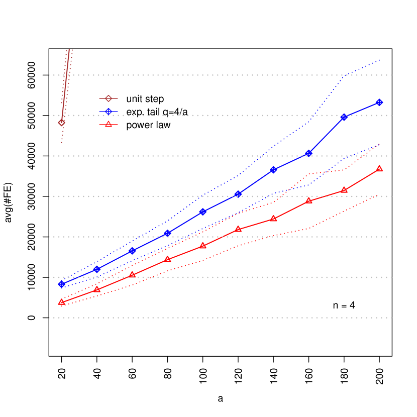
Second scenario.
Given the results from the first scenario, we fix here. We now range from to in steps of . Our results are depicted in Figure 1.
We see that the runtime for exponential-tail mutation is essentially linear, which is what we expected. However, we also see that the runtime for power-law mutation is roughly linear, which is far better than our theoretical bounds.
One explanation for this discrepancy is that our theoretical analyses always assume that the algorithm’s population is maximal, that is, it contains individuals. This assumption seems to be too pessimistic, given preliminary empirical results. In phase , if a mutation performs a larger change to an individual, this new individual is likely to strictly dominate multiple solutions in the current population, thus reducing the population size. This potentially speeds up the first phase. In phase , for similar reasons, the initial population can be small and only grows large once almost the entire Pareto front is covered. Working with smaller populations in between can reduce the runtime of the second phase.
Conclusion
In this work, we initiated the runtime analysis of multi-objective evolutionary algorithms for unbounded integer spaces. To this end, we considered variants of the well-known SEMO and GSEMO algorithms. For each algorithm, we analyzed three different distributions of their mutation strengths. We derived runtime guarantees for a simple bi-objective problem with Pareto front of size . Our theoretical results show a complex parameter landscape, depending on the different characteristics of the problem – namely, the problem size and – and of the algorithm – namely, the mutation strength.
For all reasonable problem parameter choices, the unit-step mutation is the worst update strength, since the progress in each dimension is always bounded by the lowest possible value. The comparison of the other two mutation strengths is more delicate. Our theoretical results suggest that the exponential-tail mutation can outperform the power-law mutation if its parameter is chosen carefully with respect to the problem parameters. However, in our experiments the power-law mutation always gave results superior to the exponential-tail mutation using a tuned parameter. Moreover, our experiments indicate a linear total runtime for both the exponential-tail and the power-law mutation (for certain parameter settings), which is a better runtime behavior for the power-law algorithm than what our upper bounds guarantee. We speculate this is a consequence of our pessimistic assumption of the algorithms’ population size always being maximum. However, we note that, to the best of our knowledge, this is how essentially any theoretical consideration of the (G)SEMO up to date operates, for example (Bian, Qian, and Tang 2018; Doerr and Zheng 2021; Dang et al. 2023). Overall, our empirical analysis indicates that either our theoretical guarantees are not tight for the power-law algorithm or that the asymptotic effects are only witnessed for larger problem sizes, noting that our empirical observations seem to hold even more clearly for larger values of . In any case, as both our theoretical and empirical results indicate that the power-law mutation has the best expected runtime for a wide range of problem parameters and starting points, and it does not require a careful parameter choice, our general recommendation is to prefer this algorithm for the optimization of problems with unbounded integer variables and no further problem-specific knowledge.
An interesting next step is to analyze whether our theoretical bounds are tight. We speculate that a more careful study of the algorithms’ population dynamics is required. Theoretical analyses of this level of detail have not been conducted for the (G)SEMO so far. Hence, more refined analysis techniques than the state of the art seem to be necessary.
Another interesting direction is to prove lower bounds for our considered settings. Such analyses can shed more light onto certain behavioral aspects of the algorithms, and they require a deeper understanding of the dynamics of the population size. Thus, they are challenging to derive but can lead to insights that suggest how to improve our upper bounds.
In addition, it would be interesting to analyze other multi-objective evolutionary algorithms, e.g., the very prominent NSGA-II (Deb et al. 2002) as well as the NSGA-III (Deb and Jain 2014), SPEA2 (Zitzler, Laumanns, and Thiele 2001), and the SMS-EMOA (Beume, Naujoks, and Emmerich 2007). Moreover, these algorithms have a more complex procedure of updating their population in comparison to that of the (G)SEMO. This can further prove more challenging. However, a comparison to other multi-objective algorithms would greatly improve our current theoretical knowledge of the unbounded integer domain.
Acknowledgments
This research benefited from the support of the FMJH Program Gaspard Monge for optimization and operations research and their interactions with data science.
References
- Adak and Witt (2024) Adak, S.; and Witt, C. 2024. Runtime analysis of a multi-valued compact genetic algorithm on generalized OneMax. In Parallel Problem Solving from Nature, PPSN 2024, Proceedings, Part III, 53–69.
- Antipov, Buzdalov, and Doerr (2022) Antipov, D.; Buzdalov, M.; and Doerr, B. 2022. Fast mutation in crossover-based algorithms. Algorithmica, 84: 1724–1761.
- Auger and Doerr (2011) Auger, A.; and Doerr, B., eds. 2011. Theory of Randomized Search Heuristics. World Scientific Publishing.
- Baswana et al. (2009) Baswana, S.; Biswas, S.; Doerr, B.; Friedrich, T.; Kurur, P. P.; and Neumann, F. 2009. Computing single source shortest paths using single-objective fitness. In Foundations of Genetic Algorithms, FOGA 2009, 59–66. ACM.
- Ben Jedidia, Doerr, and Krejca (2024) Ben Jedidia, F.; Doerr, B.; and Krejca, M. S. 2024. Estimation-of-distribution algorithms for multi-valued decision variables. Theoretical Computer Science, 1003: 114622.
- Beume, Naujoks, and Emmerich (2007) Beume, N.; Naujoks, B.; and Emmerich, M. 2007. SMS-EMOA: Multiobjective selection based on dominated hypervolume. European Journal of Operational Research, 181: 1653–1669.
- Bian, Qian, and Tang (2018) Bian, C.; Qian, C.; and Tang, K. 2018. A general approach to running time analysis of multi-objective evolutionary algorithms. In International Joint Conference on Artificial Intelligence, IJCAI 2018, 1405–1411. IJCAI.
- Bian et al. (2024) Bian, C.; Ren, S.; Li, M.; and Qian, C. 2024. An archive can bring provable speed-ups in multi-objective evolutionary algorithms. In International Joint Conference on Artificial Intelligence, IJCAI 2024, 6905–6913. ijcai.org.
- Cerf et al. (2023) Cerf, S.; Doerr, B.; Hebras, B.; Kahane, J.; and Wietheger, S. 2023. The first proven performance guarantees for the Non-Dominated Sorting Genetic Algorithm II (NSGA-II) on a combinatorial optimization problem. In International Joint Conference on Artificial Intelligence, IJCAI 2023, 5522–5530. ijcai.org.
- Cormen et al. (2001) Cormen, T. H.; Leiserson, C. E.; Rivest, R. L.; and Stein, C. 2001. Introduction to Algorithms. The MIT Press, 2 edition.
- Corus, Oliveto, and Yazdani (2021) Corus, D.; Oliveto, P. S.; and Yazdani, D. 2021. Fast immune system-inspired hypermutation operators for combinatorial optimization. IEEE Transactions on Evolutionary Computation, 25: 956–970.
- Dang et al. (2022) Dang, D.; Eremeev, A. V.; Lehre, P. K.; and Qin, X. 2022. Fast non-elitist evolutionary algorithms with power-law ranking selection. In Genetic and Evolutionary Computation Conference, GECCO 2022, 1372–1380. ACM.
- Dang et al. (2023) Dang, D.-C.; Opris, A.; Salehi, B.; and Sudholt, D. 2023. A proof that using crossover can guarantee exponential speed-ups in evolutionary multi-objective optimisation. In Conference on Artificial Intelligence, AAAI 2023, 12390–12398. AAAI Press.
- Deb and Jain (2014) Deb, K.; and Jain, H. 2014. An Evolutionary Many-Objective Optimization Algorithm Using Reference-Point-Based Nondominated Sorting Approach, Part I: Solving Problems With Box Constraints. IEEE Transactions on Evolutionary Computation, 18: 577–601.
- Deb et al. (2002) Deb, K.; Pratap, A.; Agarwal, S.; and Meyarivan, T. 2002. A fast and elitist multiobjective genetic algorithm: NSGA-II. IEEE Transactions on Evolutionary Computation, 6: 182–197.
- Dinot et al. (2023) Dinot, M.; Doerr, B.; Hennebelle, U.; and Will, S. 2023. Runtime analyses of multi-objective evolutionary algorithms in the presence of noise. In International Joint Conference on Artificial Intelligence, IJCAI 2023, 5549–5557. ijcai.org.
- Do et al. (2023) Do, A. V.; Neumann, A.; Neumann, F.; and Sutton, A. M. 2023. Rigorous runtime analysis of MOEA/D for solving multi-objective minimum weight base problems. In Advances in Neural Information Processing Systems, NeurIPS 2023.
- Doerr (2019) Doerr, B. 2019. Analyzing randomized search heuristics via stochastic domination. Theoretical Computer Science, 773: 115–137.
- Doerr (2020) Doerr, B. 2020. Probabilistic tools for the analysis of randomized optimization heuristics. In Doerr, B.; and Neumann, F., eds., Theory of Evolutionary Computation: Recent Developments in Discrete Optimization, 1–87. Springer. Also available at https://arxiv.org/abs/1801.06733.
- Doerr and Doerr (2018) Doerr, B.; and Doerr, C. 2018. Optimal static and self-adjusting parameter choices for the genetic algorithm. Algorithmica, 80: 1658–1709.
- Doerr, Doerr, and Kötzing (2018) Doerr, B.; Doerr, C.; and Kötzing, T. 2018. Static and self-adjusting mutation strengths for multi-valued decision variables. Algorithmica, 80: 1732–1768.
- Doerr, Doerr, and Kötzing (2019) Doerr, B.; Doerr, C.; and Kötzing, T. 2019. Solving problems with unknown solution length at almost no extra cost. Algorithmica, 81: 703–748.
- Doerr, Doerr, and Yang (2020) Doerr, B.; Doerr, C.; and Yang, J. 2020. Optimal parameter choices via precise black-box analysis. Theoretical Computer Science, 801: 1–34.
- Doerr, Happ, and Klein (2012) Doerr, B.; Happ, E.; and Klein, C. 2012. Crossover can provably be useful in evolutionary computation. Theoretical Computer Science, 425: 17–33.
- Doerr, Johannsen, and Schmidt (2011) Doerr, B.; Johannsen, D.; and Schmidt, M. 2011. Runtime analysis of the (1+1) evolutionary algorithm on strings over finite alphabets. In Foundations of Genetic Algorithms, FOGA 2011, 119–126. ACM.
- Doerr, Krejca, and Rudolph (2024) Doerr, B.; Krejca, M. S.; and Rudolph, G. 2024. Runtime Analysis for Multi-Objective Evolutionary Algorithms in Unbounded Integer Spaces (Code). Zenodo. https://zenodo.org/records/14506854.
- Doerr, Krejca, and Vu (2024) Doerr, B.; Krejca, M. S.; and Vu, N. 2024. Superior genetic algorithms for the target set selection problem based on power-law parameter choices and simple greedy heuristics. In Genetic and Evolutionary Computation Conference, GECCO 2024. ACM.
- Doerr et al. (2017) Doerr, B.; Le, H. P.; Makhmara, R.; and Nguyen, T. D. 2017. Fast genetic algorithms. In Genetic and Evolutionary Computation Conference, GECCO 2017, 777–784. ACM.
- Doerr and Neumann (2020) Doerr, B.; and Neumann, F., eds. 2020. Theory of Evolutionary Computation—Recent Developments in Discrete Optimization. Springer. Also available at http://www.lix.polytechnique.fr/Labo/Benjamin.Doerr/doerr˙neumann˙book.html.
- Doerr and Pohl (2012) Doerr, B.; and Pohl, S. 2012. Run-time analysis of the (1+1) evolutionary algorithm optimizing linear functions over a finite alphabet. In Genetic and Evolutionary Computation Conference, GECCO 2012, 1317–1324. ACM.
- Doerr and Qu (2023) Doerr, B.; and Qu, Z. 2023. A first runtime analysis of the NSGA-II on a multimodal problem. IEEE Transactions on Evolutionary Computation, 27: 1288–1297.
- Doerr and Rajabi (2023) Doerr, B.; and Rajabi, A. 2023. Stagnation detection meets fast mutation. Theoretical Computer Science, 946: 113670.
- Doerr and Zheng (2021) Doerr, B.; and Zheng, W. 2021. Theoretical analyses of multi-objective evolutionary algorithms on multi-modal objectives. In Conference on Artificial Intelligence, AAAI 2021, 12293–12301. AAAI Press.
- Friedrich, Quinzan, and Wagner (2018) Friedrich, T.; Quinzan, F.; and Wagner, M. 2018. Escaping large deceptive basins of attraction with heavy-tailed mutation operators. In Genetic and Evolutionary Computation Conference, GECCO 2018, 293–300. ACM.
- Giel (2003) Giel, O. 2003. Expected runtimes of a simple multi-objective evolutionary algorithm. In Congress on Evolutionary Computation, CEC 2003, 1918–1925. IEEE.
- Giel and Lehre (2010) Giel, O.; and Lehre, P. K. 2010. On the effect of populations in evolutionary multi-objective optimisation. Evolutionary Computation, 18: 335–356.
- Harder et al. (2024) Harder, J. G.; Kötzing, T.; Li, X.; Radhakrishnan, A.; and Ruff, J. 2024. Run Time Bounds for Integer-Valued OneMax Functions. In Genetic and Evolutionary Computation Conference, GECCO 2024, 1569–1577. ACM.
- He and Yao (2004) He, J.; and Yao, X. 2004. A study of drift analysis for estimating computation time of evolutionary algorithms. Natural Computing, 3: 21–35.
- Jansen (2013) Jansen, T. 2013. Analyzing Evolutionary Algorithms – The Computer Science Perspective. Springer.
- Johannsen (2010) Johannsen, D. 2010. Random Combinatorial Structures and Randomized Search Heuristics. Ph.D. thesis, Universität des Saarlandes.
- Kötzing and Krejca (2019) Kötzing, T.; and Krejca, M. S. 2019. First-hitting times under drift. Theoretical Computer Science, 796: 51–69.
- Kötzing, Lissovoi, and Witt (2015) Kötzing, T.; Lissovoi, A.; and Witt, C. 2015. (1+1) EA on Generalized Dynamic OneMax. In Foundations of Genetic Algorithms, FOGA 2015, 40–51. ACM.
- Krejca and Witt (2024) Krejca, M. S.; and Witt, C. 2024. A flexible evolutionary algorithm with dynamic mutation rate archive. In Genetic and Evolutionary Computation Conference, GECCO 2024, 1578–1586. ACM.
- Laumanns et al. (2002) Laumanns, M.; Thiele, L.; Zitzler, E.; Welzl, E.; and Deb, K. 2002. Running time analysis of multi-objective evolutionary algorithms on a simple discrete optimization problem. In Parallel Problem Solving from Nature, PPSN 2002, 44–53. Springer.
- Mitavskiy, Rowe, and Cannings (2009) Mitavskiy, B.; Rowe, J. E.; and Cannings, C. 2009. Theoretical analysis of local search strategies to optimize network communication subject to preserving the total number of links. International Journal on Intelligent Computing and Cybernetics, 2: 243–284.
- Neumann and Witt (2010) Neumann, F.; and Witt, C. 2010. Bioinspired Computation in Combinatorial Optimization – Algorithms and Their Computational Complexity. Springer.
- Qian et al. (2018a) Qian, C.; Shi, J.; Tang, K.; and Zhou, Z. 2018a. Constrained monotone -submodular function maximization using multiobjective evolutionary algorithms with theoretical guarantee. IEEE Transactions on Evolutionary Computation, 22: 595–608.
- Qian et al. (2018b) Qian, C.; Zhang, Y.; Tang, K.; and Yao, X. 2018b. On multiset selection with size constraints. In Conference on Artificial Intelligence, AAAI 2018, 1395–1402. AAAI Press.
- Ren et al. (2024) Ren, S.; Bian, C.; Li, M.; and Qian, C. 2024. A first running time analysis of the Strength Pareto Evolutionary Algorithm 2 (SPEA2). In Parallel Problem Solving from Nature, PPSN 2024, Part III, 295–312. Springer.
- Rudolph (1994) Rudolph, G. 1994. An evolutionary algorithm for integer programming. In Parallel Problem Solving from Nature, PPSN 1994, 139–148.
- Rudolph (2023) Rudolph, G. 2023. Runtime analysis of (1+1)-EA on a biobjective test function in unbounded integer search space. In IEEE Symposium Series on Computational Intelligence, SSCI 2023, 1380–1385. IEEE.
- Scharnow, Tinnefeld, and Wegener (2004) Scharnow, J.; Tinnefeld, K.; and Wegener, I. 2004. The analysis of evolutionary algorithms on sorting and shortest paths problems. Journal of Mathematical Modelling and Algorithms, 3: 349–366.
- Sudholt and Thyssen (2012) Sudholt, D.; and Thyssen, C. 2012. A simple ant colony optimizer for stochastic shortest path problems. Algorithmica, 64: 643–672.
- Zheng and Doerr (2024) Zheng, W.; and Doerr, B. 2024. Runtime analysis of the SMS-EMOA for many-objective optimization. In Conference on Artificial Intelligence, AAAI 2024, 20874–20882. AAAI Press.
- Zheng et al. (2024) Zheng, W.; Li, M.; Deng, R.; and Doerr, B. 2024. How to use the Metropolis algorithm for multi-objective optimization? In Conference on Artificial Intelligence, AAAI 2024, 20883–20891. AAAI Press.
- Zheng, Liu, and Doerr (2022) Zheng, W.; Liu, Y.; and Doerr, B. 2022. A first mathematical runtime analysis of the Non-Dominated Sorting Genetic Algorithm II (NSGA-II). In Conference on Artificial Intelligence, AAAI 2022, 10408–10416. AAAI Press.
- Zhou, Yu, and Qian (2019) Zhou, Z.-H.; Yu, Y.; and Qian, C. 2019. Evolutionary Learning: Advances in Theories and Algorithms. Springer.
- Zitzler, Laumanns, and Thiele (2001) Zitzler, E.; Laumanns, M.; and Thiele, L. 2001. SPEA2: Improving the strength Pareto evolutionary algorithm. TIK report, 103.
Appendix
The section titles here share the same names as in the submission.
Useful Properties of the Benchmark Problem
Proof of Lemma 1.
We begin by showing the first claim. To this end, note that by the triangle inequality and by , we have , which is equivalent to . Furthermore, as by assumption, it holds that . Combining these two statements yields .
Moreover, note that for any , by the definition of , it holds that . Using this as well as the assumption and the inequality from the previous paragraph yields that , proving the first claim.
For the second claim, note that, by the definition of , for all , it holds that . Hence, , and the first claim yields , that is, and thus . ∎
Proof of Lemma 2.
By the definition of the algorithms, only contains incomparable solutions. By Lemma 1, any two solutions from are comparable, and so are any from . ∎
Proof of Lemma 3.
For , the claim follows from Lemma 2. For and for all with , it holds that as well and thus as well as . Consequently, and are comparable. Since, by the definition of the algorithms, only contains incomparable solutions, it follows that contains at most one solution from . ∎
Proof of Lemma 4.
Proof of Lemma 5.
We prove this statement by contradiction. Hence, assume that . By the definition of and the assumption , it follows that
| (2) | ||||
Furthermore, by the assumption , it follows that
| (3) | ||||
Combining equations (2) and (3), canceling , and rearranging some terms yields
We show that this system of inequalities is infeasible, resulting in the contradiction that concludes the proof. Recall that . First, if , then the first inequality simplifies to , which is a contradiction, since, by the triangle inequality, it holds that . Last, if , then the second inequality simplifies to , which is also a contradiction, again by the triangle inequality, concluding the proof. ∎
Unit-Step Mutation
Proof of Lemma 10.
For both algorithms, we aim to apply the additive drift theorem (Theorem 8) to the process that considers the smallest L1-distance of an individual in the population to the all-s vector , that is, we consider . Note that . We consider the natural filtration of . Note that is adapted to this filtration. Furthermore, for the following, let and assume that is true.
For either algorithm, by Lemma 6, cannot increase. Hence, it suffices to consider the cases in which decreases. For to decrease, it is sufficient that the algorithm chooses the individual that is closest to and changes exactly one of the values that is not yet. For both algorithms, by Lemma 4, choosing the correct individual has a probability of at least . Still for both algorithms, the probability that the mutation chooses one of the positions that need to be improved and chooses the correct direction for improvement is at least . For the GSEMO only, we furthermore consider the event that the mutation does not change any of the other probabilities, which occurs with probability at least . All of these probabilities are mutually independent. Hence, for the SEMO, we get , and for the GSEMO . Applying the additive drift theorem, noting that , which implies that , concludes the proof. ∎
Proof of Lemma 11.
For either algorithm, we aim to apply the additive drift theorem (Theorem 8) to the random process that measures the difference of the size of the current Pareto front to the size of the maximum-cardinality Pareto front of . In other words, we consider , noting that , as contains at least the all-s vector, which is in . Furthermore, note that . We consider the filtration that is the smallest possible containing the natural filtration of , of , and of , noting that is adapted to this filtration. Last, in the following, let , and assume that is true.
Note that cannot increase, as points on the global Pareto front are never removed, due to the definition of the algorithms.
For either algorithm, since we assume that , due to our assumption on , there is at least one point in that is not in . We consider one such point that is closest to a point in . Note that such a point is in distance in the first component, as all other components are . In order for either algorithm to add this point to its current population, the algorithm needs to pick an individual from closest to , the independent probability of which is at least , due to Lemma 4. Afterward, the mutation needs to choose to change the first position in the correct way. For either algorithm, the independent probability to do so is . Last, only for the GSEMO, no other position must be changed during mutation, which occurs independently with probability . Overall, for the SEMO, we get , and for the GSEMO . Applying the additive drift theorem, using the bound on given at the beginning of the proof, and taking the conditional expected value of the result with respect to and completes the proof. ∎
Exponential-Tail Mutation
Our analysis makes use of the following lemma.
Lemma 20.
For and , it holds that
Proof of Lemma 20.
As well known, . Differentiation w.r.t. on both sides leads to
proving the first equation.
For the second equation, we use the first one and get
proving the second equation. ∎
Proof of Lemma 13.
Let temporarily to ease notation. Using the first equation from Lemma 20 and multiplying with yields
Replacing finally delivers the desired result for .
As for the bounds, first note that is monotonically decreasing on so that for . Using the (strong) Weierstrass product inequality we get and finally
Assume so that . Insertion of all bounds yields
with .
Now assume , so that . In order to get the bound we must show that is bounded from below by a constant independent from and . Note that, regardless how we choose , the value of must be at least . If we fix and increase then since . Thus, with we choose the lowest admissible value for and hence also the smallest value of , namely , which is monotonically increasing in as can be seen from the derivative. As a consequence, we get the smallest value for the limit : . Putting all together, we obtain
where the right-hand side is constant. ∎
Proof of Lemma 14.
For any population , let . For any iteration , let be the population of the SEMO or GSEMO at the start of some iteration . In the following, we analyze the effect of one iteration. Hence fix any time and any outcome of the population (hence we condition on in the following).
We estimate the expected progress (the drift) . Let with minimal. By Lemma 6 we know that if , then in the -th iteration an individual was generated with . Consequently, we have with probability one. By Lemma 4, we have . Consequently, with probability at least , the parent chosen in this iteration equals . Conditional also on this event, we estimate the drift by regarding separately two cases. To this aim, let be the constant which exists according to Lemma 13.
Case 1: If there is an such that , then with probability at least (SEMO) or (GSEMO) exactly the -th component of is changed in the mutation. If this happens, by Lemma 13, the resulting offspring satisfies . Consequently, in this first case we have regardless of whether the SEMO or GSEMO is used.
Case 2: If for all , then we argue as follows. We only regard the progress made from mutating a single position. If this position is , then by Lemma 13 again, the expected progress is at least . The probability that exactly the -th position is mutated, is again at least (SEMO) or (GSEMO). Consequently, we have . By the classic inequality relating the arithmetic and the quadratic mean (a special case of the Cauchy–Schwarz inequality), we have .
Putting all together, including the probability of selecting as parent, we have
Since is the first time that , we can apply the variable drift theorem (Theorem 7) to the process and obtain
where we used that . ∎
Proof of Lemma 15.
Let . Let . For , let and . Let . Then . For , let . Then .
Our proof strategy is to first analyze the time until for each there is at least one such that and then analyze the time until all are contained in the population. We note that all elements of the are Pareto optima, and the unique ones with their objective value, so once such a solution is contained in the population of the (G)SEMO, it will stay there forever.
For the first part, consider and a time such that , , and . Note that . We estimate the probability that . Let . By symmetry, we can assume, without loss of generality, that . By construction, there is a , determined by the position of in , such that . Consequently, if is selected as parent for the mutation operation, if only the first component of is modified, and this by increasing it by between and , then the offspring is contained in . By Lemma 4, the probability of this event is at least , where is such that a bilateral geometric random variable with parameter satisfies for all . Recalling that , we note that for all considered, so is a feasible choice (note that here we used that for all ). Consequently, the expected time until is the reciprocal of this probability, that is, . Since we start with , using the above argument times (for suitable values of and ), we see that the expected to have for all is .
We now analyze how the population fills up the blocks , . Note that we can assume that as otherwise we are done already. We first regard an arbitrary fixed block , . Assume that at some time , this block contains at least one individual from . Fixing such an initial situation, we analyze the time until the population contains . Let be some individual in the current population and in and let be an element of not contained in the current population. For both the SEMO and the GSEMO, the probability that a mutation operation with as parent mutates into is at least ; here denotes a bilateral geometric random variable with parameter and the last estimate uses again that for all . As this bound is independent of and , a simple union bound over the choices of and the choices of , with the lower bound of for picking a particular as parent, yields that with probability at least
this iteration increases the number of individuals in from to . This estimate is valid for any state of the population as long as there are exactly individuals in . Consequently, the time to go from to individuals is stochastically dominated (see, e.g., (Doerr 2019) for some background on stochastic domination) by a geometric random variable with success rate , and the time to go from our arbitrary initial state with at least one individual in to a state with fully contained in the population is stochastically dominated by the sum of independent geometric random variables with success rates , , that is, .
We note that for , we have , whereas for , we have . Let be two independent random variables, each being the independent sum of geometric random variables with success rates . Then . We note that the , fulfill the assumptions of the Chernoff bound for geometric random variables proven in (Doerr and Doerr 2018, Lemma 4) (which is Theorem 1.10.35 in (Doerr 2020)). Consequently,
for all and . Using a simple union bound, we derive
Let . Then a union bound over the shows that with probability at least , all are contained in the population after time steps. Repeating this argument, we see that after an expected number of iterations, all are contained in the population, that is, the population contains the Pareto set.
Putting the two phases together, we see that
where the last estimate follows from noting, via a case distinction, that . ∎
Power-Law Mutation
Proof of Lemma 18.
We consider the smallest distance of the population to , that is, we consider where, for all , we have . Note that is the first point in time such that . We aim to apply the variable drift theorem (Theorem 7) to .
To this end, consider an iteration such that . By Lemma 6, the minimum L1-norm in the population cannot increase. Hence, using the notation of Algorithm 1, we consider the case that we choose such that and that the offspring is such that . Let denote the event that we choose such an . By Lemma 4, the probability of is at least .
We first consider the drift in component of . SEMO chooses to mutate (only) this position independently with probability at least , and GSEMO does so with probability at least . Afterward, with probability , the change by the mutation has the correct sign such that moves toward . Any change by results in an improvement by in component . Applying Theorem 17, the expected change in component is then at least
| (4) | ||||
Since the expected progress in the L1-norm is the sum of the progresses over the components, we obtain
We derive a lower bound for the right-hand side. Since , the function is concave, and since we consider a sum of such concave functions, the sum is also concave. A concave function takes its minimum at the border of a bounded set. Hence, this expression is minimized if a single component has all the mass, that is, if there is an such that . Thus,
We further bound this expression from below by a case distinction.
If , then , and thus . As and , this results in
For , we consider only the sum in equation (4) for , resulting in
Since the drift is monotonically non-decreasing in , we apply the variable drift theorem (Theorem 7). To this end, we apply a case distinction with respect to whether , we account for the probability of derived at the beginning of the proof, and we apply Theorem 17. We obtain
Removing the term and noting that concludes the proof. ∎
Proof of Lemma 19.
If , then . Hence, we assume in the following that . We consider several steps until at least a half of is covered. Afterward, we consider one more stage such that is fully covered.
For step with , consider a partition of into consecutive intervals of roughly equal size and such that at least of them contain at least one individual in the current population (called hit). Formally, let , noting that is never integer and that . We consider the partitioning of into . Step ends once all intervals are hit. Note that due to the assumption about , the constraints for step are satisfied in iteration .
Consider step . Each interval has a size of at most . Since we halve the intervals from the previous step (or the entire interval if ), each interval that is not hit yet is neighboring at least one interval that is already hit. Hence, in the worst case, in order to create any individual in an unhit interval, a distance of at least needs to be overcome from the neighboring interval that contains an individual. Each point in an unhit interval (of which there are at least ) is a possible target in order to hit the interval.
The previous discussion implies that in order to hit an unhit interval , the following sequence of events is sufficient. First, choose a parent from a hit neighbor, which has, by Lemma 4, a probability of at least , and then mutate the first component of the parent, which happens for the SEMO with probability at least and for the GSEMO with probability at least . Afterward, the mutation needs to adjust the first component into the correct direction, which happens with probability . Since all of these decisions are independent, this results in a probability of at least for choosing a specific parent and mutating it into a direction such that it can hit . We call this chain of events . Such an individual can be mutated in at least ways in its first component, needing to hit a distance of at least . Conditional on , we bound the probability that the mutation results in an offspring that hits from below. To this end, we use Theorem 17, that , as is not integer, and that , as . We obtain
Overall, accounting for the probability of , the probability that a mutation covers is at least
The probability that interval is not covered within iterations is at most . Hence, the probability to cover all uncovered intervals within iterations is, by Bernoulli’s inequality, at least . By a restart argument, step lasts in expectation at most iterations.
Summing over all steps from to , we get that the total expected length of all steps. To this end, we use the notation as well as Lemma 20. We an upper bound of
Afterward, at least half of is covered.
We continue with the last stage. Let denote the number of solutions from that are still not in the population. Note that by the previous sequence of steps, each such solution not in the population has at least one neighbor in the population in distance . Hence, the probability to add a new solution to the population is at least . The expected time until a new solution is added is the multiplicative inverse of this probability. Hence, the total expected time of the last stage is bounded from above by
The proof is concluded by noting that is bounded from above by the estimate of the two sums above. ∎
Empirical Analysis
We follow the same experimental setup as in the main paper but for the values of . For the initial solution, we choose and all of the other components of as .
First scenario.
Our results are depicted in Table 2. The results are qualitatively comparable to those in Table 1. That is, the step size of is best in terms of total runtime for the exponential-tail mutation. For , the relative difference between and is very small, which is why we choose for consistency reasons with also for for the second scenario.
The runtime of the power-law mutation for either of the two phases we consider is better than any of those of the exponential-tail mutation. Unit-step mutation performs by far the worst.
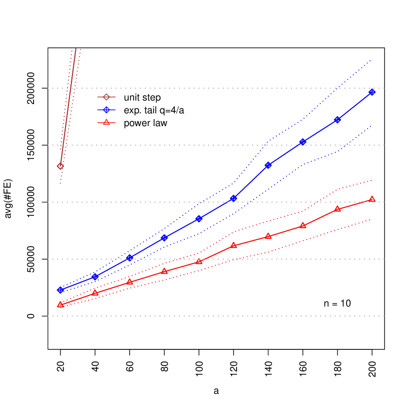
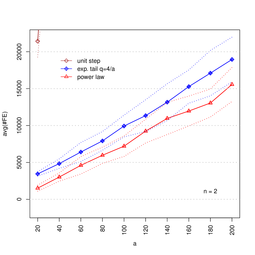
Second scenario.
Our results are depicted in Figure 2. As in our results for (Figure 1), unit-step mutation performs by far the worst, with exponential-tail and power-law mutation performing both roughly linearly. The separation between exponential-tail mutation and power-law mutation becomes more distinct with increasing values of , to the extent where the standard deviations do not intersect anymore for . This indicates a clear advantage of the power-law mutation for increasing values of .
| 1st hit | cover | total | |||||
|---|---|---|---|---|---|---|---|
| U | 850 395 | 31 | 995 144 | 34 | 1 845 539 | 13 | |
| \hdashlineE | 5 | 164 192 | 11 | 607 63 | 33 | 224 955 | 10 |
| 10 | 56 364 | 10 | 43 821 | 22 | 100 185 | 10 | |
| 20 | 21 782 | 10 | 38 192 | 15 | 59 974 | 11 | |
| 50 | 10 701 | 29 | 40 518 | 17 | 51 219 | 16 | |
| 100 | 13 813 | 47 | 48 918 | 17 | 62 731 | 18 | |
| 200 | 21 745 | 50 | 65 441 | 18 | 87 186 | 23 | |
| 500 | 48 866 | 54 | 113 862 | 17 | 162 728 | 22 | |
| \hdashlineP | 2 678 | 38 | 34 075 | 18 | 36 753 | 17 | |
| 1st hit | cover | total | |||||
|---|---|---|---|---|---|---|---|
| U | 1 792 117 | 31 | 2 467 353 | 36 | 4 259 470 | 12 | |
| \hdashlineE | 5 | 458 488 | 8 | 167 105 | 32 | 625 593 | 10 |
| 10 | 162 492 | 8 | 113 735 | 20 | 276 227 | 9 | |
| 20 | 77 547 | 12 | 108 167 | 16 | 185 715 | 9 | |
| 50 | 74 820 | 18 | 123 049 | 22 | 197 869 | 17 | |
| 100 | 113 681 | 21 | 139 902 | 17 | 253 583 | 13 | |
| 200 | 186 919 | 25 | 183 954 | 15 | 370 872 | 16 | |
| 500 | 379 859 | 32 | 321 510 | 11 | 701 369 | 18 | |
| \hdashlineP | 8 516 | 35 | 93 739 | 17 | 102 255 | 17 | |