Soft and Constrained Hypertree Width

Abstract.

Hypertree decompositions provide a way to evaluate Conjunctive Queries (CQs) in polynomial time, where the exponent of this polynomial is determined by the width of the decomposition. In theory, the goal of efficient CQ evaluation therefore has to be a minimisation of the width. However, in practical settings, it turns out that there are also other properties of a decomposition that influence the performance of query evaluation. It is therefore of interest to restrict the computation of decompositions by constraints and to guide this computation by preferences. To this end, we propose a novel framework based on candidate tree decompositions, which allows us to introduce soft hypertree width (shw). This width measure is a relaxation of hypertree width (hw); it is never greater than hw and, in some cases, shw may actually be lower than hw. Most importantly, shw preserves the tractability of deciding if a given CQ is below some fixed bound, while offering more algorithmic flexibility. In particular, it provides a natural way to incorporate preferences and constraints into the computation of decompositions. A prototype implementation and preliminary experiments confirm that this novel framework can indeed have a practical impact on query evaluation.

1. Introduction

Since their introduction nearly 25 years ago, hypertree decompositions (HDs) and hypertree width ($\mathit{hw}$) have emerged as a cornerstone in the landscape of database research. Their enduring relevance lies in their remarkable ability to balance theoretical elegance with practical applicability. Hypertree width generalises $\alpha$-acyclicity, a foundational concept for the efficient evaluation of conjunctive queries (CQs) (DBLP:conf/vldb/Yannakakis81, ). Indeed, CQs of bounded hypertree width can be evaluated in polynomial time. Crucially, determining whether a CQ has $\mathit{hw}\leq k$ for fixed $k\geq 1$ and, if so, constructing an HD of width $\leq k$ can also be achieved in polynomial time (GLS, ).

Over the decades, hypertree width has inspired the development of generalised hypertree width ($\mathit{ghw}$) (ghw3, ) and fractional hypertree width ($\mathit{fhw}$) (fhw, ), each extending the boundaries of tractable CQ evaluation. These generalisations induce larger classes of tractable CQs. Notably, the hierarchy

$$\mathit{fhw}(q)\leq\mathit{ghw}(q)\leq\mathit{hw}(q)$$

holds for any CQ q, with the respective width measure determining the exponent of the polynomial bound on the query evaluation time. Consequently, practitioners naturally gravitate towards width measures that promise the smallest possible decomposition widths. Despite this motivation, HDs and $\mathit{hw}$ retain a crucial distinction: $\mathit{hw}$ is, to date, the most general width measure for it can be decided in polynomial time (GLS, ) if the width of a given query is below some fixed bound $k$. By contrast, generalised and fractional hypertree width, while often yielding smaller width values, suffer from computational intractability in their exact determination (ghw3, ; JACM, ). In this work, we introduce a novel width notion—soft hypertree width ($\mathit{shw}$) – that overcomes this trade-off by retaining polynomial-time decidability while potentially reducing widths compared to $\mathit{hw}$.

But this is only a first step towards a larger goal. Query evaluation based on decomposition methods works via a transformation of a given CQ with low width into an acyclic CQ by computing “local” joins for the bags at each node of the decomposition. The acyclic CQ is then evaluated by Yannakakis’ algorithm (DBLP:conf/vldb/Yannakakis81, ). From a theoretical perspective, the complexity of this approach solely depends on the width, while the actual cost of the local joins and the size of the relations produced by these joins is ignored. To remedy this short-coming, Scarcello et al. (DBLP:journals/jcss/ScarcelloGL07, ) introduced weighted HDs to incorporate costs into HDs. More precisely, among the HDs with minimal width, they aimed at an HD that minimises the cost of the local joins needed to transform the CQ into an acyclic one and the cost of the (semi-)joins required by Yannakakis’ algorithm. Promising first empirical results were obtained with this approach.

However, there is more to decomposition-based query optimisation than minimising the width. For instance, $\mathit{hw}=2$ means that we have to compute joins of two relations to transform the given query into an acyclic one. Regarding width, it makes no difference if the join is a Cartesian product of two completely unrelated relations or a comparatively cheap join along a foreign key relationship. This phenomenon is, in fact, confirmed by Scarcello et al. (DBLP:journals/jcss/ScarcelloGL07, ) when they report on decompositions with higher width but lower cost in their experimental results. Apart from the pure join costs at individual nodes or between neighbouring nodes in the decomposition, there may be yet other reasons why a decomposition with slightly higher width should be preferred. For instance, in a distributed environment, it makes a huge difference, if the required joins and semi-joins are between relations on the same server or on different servers. In other words, apart from incorporating costs of the joins at a node and between neighbouring nodes in the HD, a more general approach that considers constraints and preferences is called for.

In this work, we propose a novel framework based on the notion of candidate tree decompositions (CTDs) from (JACM, ). A CTD is a tree decomposition (TD) whose bags have to be chosen from a specified set of vertex sets (= the candidate bags). One can then reduce the problem of finding a particular decomposition (in particular, generalised or fractional hypertree decomposition) for given CQ $q$ to the problem of finding a CTD for an appropriately defined set of candidate bags. In (JACM, ), this idea was used (by specifying appropriate sets of candidate bags) to identify tractable fragments of deciding, for given CQ $q$ and fixed $k$, if $\mathit{ghw}(H)\leq k$ or $\mathit{fhw}(H)\leq k$ holds. However, as was observed in (JACM, ), it is unclear how the idea of CTDs could be applied to $\mathit{hw}$-computation, where parent/child relationships between nodes in a decomposition are critical.

We will overcome this problem by introducing a relaxed notion of HDs and $\mathit{hw}$, which we will refer to as soft HDs and soft $\mathit{hw}$ ($\mathit{shw}$). The crux of this approach will be a relaxation of the so-called “special condition” of HDs (formal definitions of all concepts mentioned in the introduction will be given in Section 2): it will be restrictive enough to guarantee a polynomial upper bound on the number of candidate bags and relaxed enough to make the approach oblivious of any parent/child relationships of nodes in the decomposition. We thus create a novel framework based on CTDs, that paves the way for several improvements over the original approach based on HDs and $\mathit{hw}$, while retaining the crucial tractability of deciding, for fixed $k$, if the width is $\leq k$ and, if so, computing a decomposition of the desired width.

First of all, $\mathit{shw}$ constitutes an improvement in terms of the width, i.e., it is never greater than $\mathit{hw}$ and there exist CQs $q$ with strictly smaller $\mathit{shw}$ then $\mathit{hw}$. The definition of soft HDs and soft $\mathit{hw}$ lends itself to a natural generalisation by specifying rules for extending a given set of candidate bags in a controlled manner. We thus define a whole hierarchy of width measures $(\mathit{shw}^{i})_{i\geq 0}$ with $\mathit{shw}^{0}=\mathit{shw}$. Moreover, will prove that $\mathit{shw}^{\infty}=\mathit{ghw}$ holds. In other words, we extend the above mentioned hierarchy of width measures to the following extended hierarchy:

$$\mathit{fhw}(q)\leq\mathit{ghw}(q)=\mathit{shw}^{\infty}(q)\leq\mathit{shw}^{i}(q)\leq\mathit{shw}^{0}(q)=\mathit{shw}(q)\leq\mathit{hw}(q),$$

which holds for every CQ $q$. Basing our new width notion $\mathit{shw}$ on CTDs gives us a lot of computational flexibility. In particular, in (JACM, ), a straightforward algorithm was presented for computing a CTD for a given set of candidate bags. We will show how various types of constraints (such as disallowing Cartesian products) and preferences (which includes the minimisation of costs functions in (DBLP:journals/jcss/ScarcelloGL07, ) as an important special case) can be incorporated into the computation of CTDs without destroying the polynomial time complexity. We emphasise that even though our focus in this work is on soft HDs and $\mathit{shw}$, the incorporation of constraints and preferences into the CTD computation equally applies to any other use of CTDs – such as the above mentioned computation of generalised and fractional hypertree decomposition in certain settings proposed in (JACM, ). We have also carried out first experimental results with a prototype implementation of our approach. In short, basing query evaluation on soft HDs and incorporating constraints and preferences into their construction may indeed lead to significant performance gains. Moreover the computation of soft HDs in a bottom-up fashion via CTDs instead of the top-down construction (DBLP:journals/jea/FischlGLP21, ; detk, ) or parallel computation of HDs (tods, ) is in the order of milliseconds and does not create a new bottleneck.

Contributions

In summary, our main contributions are as follows:

• We introduce a new type of decompositions plus associated width measure for CQs – namely soft hypertree decompositions and soft hypertree width. We show that this new width measure $\mathit{shw}$ retains the tractability of $\mathit{hw}$, it can never get greater than $\mathit{hw}$ but, in some cases, it may get smaller. Moreover. we generalise $\mathit{shw}$ to a whole hierarchy $(\mathit{shw}^{i})_{i\geq 0}$ of width measures that interpolates the space between $\mathit{hw}$ and $\mathit{ghw}$.

• The introduction of our new width measures is made possible by dropping the “special condition” of HDs. This allows us the use of candidate TDs, which brings a lot of computational flexibility. We make use of this added flexibility by incorporating constraints and preferences in a principled manner into the computation of decompositions. These ideas of extending the computation of decompositions is not restricted to $\mathit{shw}$ but is equally beneficial to $\mathit{ghw}$ and $\mathit{fhw}$ computation.

• We have implemented our framework. Preliminary experiments with our prototype implementation have produced promising results. In particular, the use of soft HDs and the incorporation of constraints and preferences into the computation of such decompositions may indeed lead to a significant performance gain in query evaluation.

Structure

The rest of this paper is structured as follows: After recalling some basic definitions and results on hypergraphs in Section 2 we revisit the notion of candidate tree decompositions from (JACM, ) in Section 3. In Section 4, we introduce the new notion of soft hypertree width $\mathit{shw}$, which is then iterated to $\mathit{shw}^{i}$ in Section 5. The integration of preferences and constraints into soft hypertree decompositions is discussed in Section 6 and first experimental results with these decompositions are reported in Section 7. Further details are provided in the appendix.

2. Preliminaries

Conjunctive queries (CQs) are first-order formulas whose only connectives are existential quantification and conjunction, i.e., $\forall,\vee$, and $\neg$ are disallowed. Likewise, Constraint Satisfaction Problems (CSPs) are given in this form. Hypergraphs have proved to be a useful abstraction of CQs and CSPs. Recall that a hypergraph $H$ is a pair $(V(H),E(H))$ where $V(H)$ is called the set of vertices and $E(H)\subseteq 2^{V(H)}$ is the set of (hyper)edges. Then the hypergraph $H(\phi)$ corresponding to a CQ or CSP given by a logical formula $\phi$ has as vertices the variables occurring in $\phi$. Moreover, every collection of variables jointly occurring in an atom of $\phi$ forms an edge in $H(\phi)$. From now on, we will mainly talk about hypergraphs with the understanding that all results equally apply to CQs and CSPs.

We write $I(v)$ for the set $\{e\in E(H)\mid v\in e\}$ of edges incident to vertex $v$. W.l.o.g., we assume that hypergraphs have no isolated vertices, i.e., every $v\in V(H)$ is in some edge. A set of vertices $U\subseteq V(H)$ induces the induced subhypergraph $H[U]$ with vertices $U$ and edges $\{e\cap U\mid e\in E(H)\}\setminus\emptyset$.

Let $H$ be a hypergraph and let $S\subseteq V(H)$. We say that two vertices $u,v$ are $[S]$-connected if they are not in $S$ and there is a path from $u$ to $v$ without any vertices of $S$. Two edges $e,f$ are $[S]$-connected if there are $[S]$-connected vertices $u\in e,v\in f$. An $[S]$-component is a maximal set of pairwise $[S]$-connected edges. For a set of edges $\lambda\subseteq E(H)$, we will simply speak of $[\lambda]$-components in place of $[\bigcup\lambda]$-components .

A tree decomposition (TD) of hypergraph $H$ is a tuple $(T,B)$ where $T$ is a tree and $B:V(T)\to 2^{V(H)}$ such that the following hold:

1. for every $e\in E(H)$, there is a node $u$ in $T$ such that $e\subseteq B(u)$,

2. and for every $v\in V(H)$, $\{u\in V(T)\mid v\in B(u)\}$ induces a non-empty subtree of $T$.

The latter condition is referred to as the connectedness condition. We sometimes assume that a tree decomposition is rooted. In this case we write $T_{u}$ for $u\in V(T)$ to refer to the subtree rooted at $u$. For subtree $T^{\prime}$ of $T$, we write $B(T^{\prime})$ for $\bigcup_{u\in V(T^{\prime})}B(u)$.

A generalised hypertree decomposition (GHD) of a hypergraph $H$ is a triple $(T,\lambda,B)$, such that $(T,B)$ is a tree decomposition and $\lambda\colon V(T)\rightarrow 2^{E(H)}$ satisfies $B(u)\subseteq\bigcup\lambda(u)$ for every $u\in V(T)$. That is, every $\lambda(u)$ is an edge cover of $B(u)$. A hypertree decomposition (HD) of a hypergraph $H$ is a GHD $(T,\lambda,B)$, where the $T$ is rooted and the so-called special condition holds, i.e., for every $u\in V(T)$, we have $B(T_{u})\cap\bigcup\lambda(u)\subseteq B(u)$. Actually, in the literature on (generalised) hypertree decompositions, it is more common to use $\chi$ instead of $B$. Moreover, rather than explicitly stating $B$, $\chi$, and $\lambda$ as functions, they are usually considered as labels – writing $B_{u},\lambda_{u}$, and $\chi_{u}$ rather than $B(u)$, $\chi(u)$, and $\lambda(u)$, and referring to them as $B$-, $\chi$-, and $\lambda$-label of node $u$.

3. Revisiting Candidate Tree Decompositions

We recall the candidate tree decomposition problem CandidateTD introduced in (JACM, ). To that end we will be interested in tree decompositions of a specific structure.

Definition 0.

A rooted tree decomposition $(T,B)$ is in component normal form (CompNF), if for each node $u\in V(T)$, and for each child $c$ of $u$, there is exactly one $[B(u)]$-edge component $C_{c}$ such that $B(T_{c})=\bigcup C_{c}\cup(B(u)\cap B(c))$. That is, each subtree “corresponds” to one $[B(u)]$-edge component plus the interface $B(u)\cap B(c)$ from the parent node $u$ into this component.

In the CandidateTD problem, we are given a hypergraph $H$ and a set $\mathbf{S}\subseteq 2^{V(H)}$ (= the set of candidate bags), and we have to decide whether there exists a CompNF tree decomposition $(T,B)$ of $H$, such that, for every node $u\in T$, we have $B(u)\in\mathbf{S}$. That is, whether a CompNF TD of $H$ can be formed using only candidate bags. We refer to such a TD as candidate tree decomposition (CTD).

1

2

3

input: Hypergraph $H$ and a set $\mathbf{S}\subseteq 2^{V(H)}$.

output: “Accept”, if there is a CompNF CTD for $\mathbf{S}$ “Reject”, otherwise.

4

5$blocks=$ all blocks headed by any $S\in\mathbf{S}\cup\{\emptyset\}$

6 foreach $(B,C)\in blocks$ do

7    if $C=\emptyset$ then  $basis(B,C)\leftarrow\emptyset$

8    else  $basis(B,C)\leftarrow\bot$ /* a block is satisfied iff its basis is not $\bot$ */

9   

10repeat

11    foreach $(B,C)\in blocks$ that are not satisfied do

12       foreach $X\in\mathbf{S}\setminus\{B\}$ do

13          if $X$ is a basis of $(B,C)$ then

14             $basis(B,C)\leftarrow X$

15            

16until no blocks changed

17if $basis(\emptyset,V(H))\neq\bot$ then

18    return Accept

19   

20return Reject

Algorithm 1 CompNF Candidate Tree Decomposition of $\mathbf{S}$

It was also shown in (JACM, ) that the problem of deciding whether a hypergraph has width $\leq k$ for various notions of decompositions can be reduced to the CandidateTD problem by an appropriate choice of the set $S$ of candidate bags. For instance, if $\mathbf{S}$ consists of the subsets of ${V(H)}$ of size at most $k+1$, then the CandidateTD problem equals checking $\mathit{tw}\leq k$; if $\mathbf{S}$ consists of sets of the form $\bigcup\lambda$ for arbitrary set $\lambda$ of at most $k$ edges of $H$, then it checks $\mathit{ghw}\leq k$. It has been shown in (JACM, ) that the CandidateTD problem is decidable in polynomial time (w.r.t. the combined size of $H$ and $\mathbf{S}$). Consequently, the CTD framework was used successfully in (JACM, ) to prove tractability results for certain kinds of decomposition problems by reducing them to the CandidateTD problem for a polynomially bounded set of candidate bags. For instance, tractability of deciding $\mathit{ghw}(H)\leq k$ and $\mathit{fhw}(H)\leq k$ for fixed $k$ (that latter denoting “fractional hypertree width” introduced in (fhw, )) for sets of hypergraphs with bounded multiple intersection has been proven in this fashion (JACM, ; DBLP:conf/mfcs/GottlobLPR20, ).

We further recall important details from (JACM, ) that will be relevant in the rest of the paper. We call a pair $(B,C)$ of disjoint subsets of $V(H)$ a block if $C$ is a maximal set of $[B]$-connected vertices of $H$ or $C=\emptyset$. We say that $(B,C)$ is headed by $B$. For two blocks $(B,C)$ and $(X,Y)$ define $(X,Y)\leq(B,C)$ if $X\cup Y\subseteq B\cup C$ and $Y\subseteq C$. A block $(B,C)$ corresponds to the subproblem of whether there exists a ComNF decomposition of $H[B\cup C]$, where the root has bag $B$. If such a decomposition exists, then we call a block satisfied. Note that if $C=\emptyset$, the block is trivially satisfied. For a block $(B,C)$ and $X\subseteq V(H)$ with $X\neq B$, we say that $X$ is a basis of $(B,C)$ if the following conditions hold:

1. Let $(X,Y_{1}),\dots,(X,Y_{\ell})$ be all the blocks headed by $X$ with $(X,Y_{i})\leq(B,C)$. Then $C\subseteq X\cup\bigcup_{i=1}^{\ell}Y_{i}$.

2. For each $e\in E(H)$ such that $e\cap C\neq\emptyset$, $e\subseteq X\cup\bigcup_{i=1}^{\ell}Y_{i}$.

3. For each $i\in[\ell]$, the block $(X,Y_{i})$ is satisfied.

To simplify later presentation, we recall the algorithm for deciding CandidateTD by Gottlob et al. (JACM, ) in a slightly adapted form in Algorithm 1. The algorithm iteratively marks satisfied blocks through bottom-up dynamic programming. Termination on Line 1 means that there is a decomposition for the full hypergraph (which can also be seen as $(\emptyset,V(H))$ being satisfied). The polynomial time upper bound follows from the observation that a depth $d$ CTD will be found after $d$ steps of the algorithm. Since a CompNF TD can have depth at most $|V(H)|$, the outer loop runs at most a linear number of times, each clearly only requiring polynomial time in $H$ and $\mathbf{S}$.

4. Soft Hypertree Width

So far, it is not known whether there is a set of candidate bags $\mathbf{S}_{H,k}$ for a hypergraph $H$ such that there is a CTD for $\mathbf{S}_{H,k}$ if and only if $\mathit{hw}(H)\leq k$. However, in (tods, ), it was shown that there always exists a HD of minimal width such that all bags of nodes $c$ with parents $p$ are of the form $B_{c}=\left(\bigcup\lambda_{c}\right)\cap\left(\bigcup C_{p}\right)$ where $C_{p}$ is a $[\lambda_{p}]$-component of $H$. In principle, this gives us a concrete way to enumerate a sufficient list of candidate bags. The number of all such bags is clearly polynomial in $H$: there are at most $|E(H)|^{k+1}$ sets of at most $k$ edges, and each of them cannot split $H$ into more than $|E(H)|$ components. The only point that is unclear when enumerating such a list of candidate bags, is how to decide beforehand whether two sets of edges $\lambda_{c},\lambda_{p}$ are in a parent/child relationship (and if so, which role they take). However, we observe that the parent/child roles are irrelevant for the polynomial bound on the number of candidate bags. Hence, we may drop this restriction and instead simply consider all such combinations induced by any two sets of at most $k$ edges. Concretely, this leads us to the following definitions.

Definition 0 (The set $\mathsf{Soft}_{H,k}$).

For hypergraph $H$, we define $\mathsf{Soft}_{H,k}$ as the set that contains all sets of the form

(1) $$B=\left(\bigcup\lambda_{1}\right)\cap\left(\bigcup C\right)$$

where $C$ is a $[\lambda_{2}]$-edge component of $H$ and $\lambda_{1},\lambda_{2}$ are sets of at most $k$ edges of $H$.

Definition 0 (Soft Hypertree Width).

A soft hypertree decomposition of width $k$ for hypergraph $H$ is a candidate tree decomposition for $\mathsf{Soft}_{H,k}$. The soft hypertree width ($\mathit{shw}$) of hypergraph $H$ is the minimal $k$ for which there exists a soft hypertree decomposition of $H$.

This measure naturally generalises the notion of hypertree width in a way that remains tractable to check (for fixed $k$), but removes the need for the special condition.

Theorem 3.

Let $k\geq 1$. Deciding, for given hypergraph $H$, whether $\mathit{shw}(H)\leq k$ holds, is feasible in polynomial time in the size of $H$. The problem even lies in the highly parallelisable class LogCFL.

Proof Sketch.

In (GLS, ), it is shown that checking if $\mathit{hw}(H)\leq k$ holds for fixed $k\geq 1$ is in LogCFL. The key part of the proof is the construction of an alternating Turing machine (ATM) that runs in Logspace and Ptime. The ATM constructs an HD in a top-down fashion. In the existential steps, one guesses a $\lambda$-label of the next node in the HD. Given the label $\lambda_{c}$ of the current node and the label $\lambda_{p}$ of its parent node, one can compute the set of $[\lambda_{c}]$-components that lie inside a $[\lambda_{p}]$-component. In the following universal step, the ATM has to check recursively if all these $\lambda_{c}$-components admit an HD of width $\leq k$.

This ATM can be easily adapted to an ATM for checking if $\mathit{shw}(H)\leq k$ holds. The main difference is, that rather than guessing the label $\lambda_{c}$ of the current node (i.e., a collection of at most $k$ edges), we now simply guess an element from $\mathsf{Soft}_{H,k}$ as the bag $B_{c}$ of the current node. The universal step is then again a recursive check for all components of $B_{c}$ that lie inside a $[B_{p}]$-component, if they admit a candidate TD of width $\leq k$. The crucial observation is that we only need Logspace to represent the bags $B\in\mathit{shw}(H)$, because every such bag is uniquely determined by the label $\lambda_{c}$ and a $[\lambda_{p}]$-component. Clearly, $\lambda_{c}$ can be represented by up to $k$ (pointers to) edges in $E(H)$, and a $[\lambda_{p}]$-component can be represented by up to $k+1$ (pointers to) edges in $E(H)$, i.e., up to $k$ edges in $\lambda_{p}$ plus 1 edge from the $[\lambda_{p}]$-component. Clearly, the latter uniquely identifies a component, since no edge can be contained in 2 components. ∎

The main argument in the proof of Theorem 3 was that the ATM for checking $\mathit{hw}(H)\leq k$ can be easily adapted to an algorithm for checking $\mathit{shw}(H)\leq k$. Actually, the straightforward adaptation of existing $\mathit{hw}$-algorithms to $\mathit{shw}$-algorithms is by no means restricted to the rather theoretical ATM of (GLS, ). Also the det-k-dedcomp algorithm presented in (detk, ) and the new-det-k-decomp algorithm used in (DBLP:journals/jea/FischlGLP21, ) for creating the HyperBench benchmark are readily turned into an $\mathit{shw}$-algorithm. We just need to replace the search for $\lambda$-labels of edges from $E(H)$ by a search for bags from $\mathsf{Soft}_{H,k}$. Note that the parallel algorithm log-k-decomp from (tods, ) (which “guesses” pairs of $\lambda$-labels for parent and child nodes and has to keep track of the orientation of each subtree of the HD to be constructed) becomes unnecessarily complex for $\mathit{shw}$-computation, where we do not need to check the special condition. Hence, we may ignore the parent/child-relationships and, in particular, the orientation of subtrees. Instead, we may follow the philosophy of the much simpler BalancedGo algorithm in (DBLP:journals/constraints/GottlobOP22, ) for $\mathit{ghw}$-computation. That is, rather than putting all bags according to Definition 1 into $\mathsf{Soft}_{H,k}$, we first only put balanced separators (i.e., $\lambda_{1}$-labels that give rise to components containing at most half of the original edges) there. Then we actually compute the components and recursively determine balanced separators for the resulting “subproblems”, etc. As with BalancedGo, we thus end up with a recursive procedure whose recursion depth is logarithmically bounded. In Section 6, we will extend the CTD-framework by constraints and preferences. It will turn out that we can thus also capture the opt-k-decomp approach from (DBLP:journals/jcss/ScarcelloGL07, ), that integrates a cost function into the computation of HDs. To conclude, the key techniques for modern decomposition algorithms are also applicable to $\mathit{shw}$-computation. Additionally, just as with other popular hypergraph width measures, it is possible to relate $\mathit{shw}$ to a (extended) variant of the Robber and Marshals game, which we present in Section A.1.

In the remainder of this section, we study the relationship between $\mathit{shw}(H)$ and $\mathit{hw}(H)$. We get the following result:

Theorem 4.

For every hypergraph $H$, the relationship $\mathit{ghw}(H)\leq\mathit{shw}(H)\leq\mathit{hw}(H)$ holds. Moreover, there exist hypergraphs $H$ with $\mathit{shw}(H)<\mathit{hw}(H)$.

Proof.

By (tods, ), if $\mathit{hw}(H)=k$, then there exists a hypertree decomposition of width $k$ such that every bag is of the form from Equation 1. That is, for every HD $(T,\lambda,\chi)$, we immediately get a candidate TD $(T,\chi)$ for $\mathsf{Soft}_{H,k}$. Hence, $\mathit{shw}(H)\leq\mathit{hw}(H)$. Furthermore, every bag in $\mathsf{Soft}_{H,k}$ is subset of a union of $k$ edges, hence $\rho(B)\leq k$ for any $B$ from Equation 1. Thus also $\mathit{ghw}(H)\leq\mathit{shw}(H)$. In the example below, we will present a hypergraph $H$ with $\mathit{shw}(H)<\mathit{hw}(H)$. ∎

We now present a hypergraph $H$ with $\mathit{shw}(H)=2$ and $\mathit{hw}(H)=3$

(a) Hypergraph $H_{2}$ with $\mathit{ghw}(H_{2})=\mathit{shw}(H_{2})=2$ and $\mathit{hw}(H_{2})=3$. Some edges are coloured for visual clarity.

(b) A soft hypertree decomposition of $H_{2}$ with width 2.

Figure 1. (a) A hypergraph $H_{2}$ and (b) its soft hypertree decomposition.

Example 0.

Let us revisit the hypergraph $H_{2}$ from (DBLP:journals/ejc/AdlerGG07, ), which was presented there to show that $\mathit{ghw}$ can be strictly smaller than $\mathit{hw}$. The hypergraph is shown in Figure 1(a). It consists of the edges $\{1,8\},\{3,4\},\{1,2,a\},\{4,5,a\},\{6,7,a\},\{2,3,b\},\{5,6,b\},\{7,8,b\}$ and no isolated vertices. It is shown in (DBLP:journals/ejc/AdlerGG07, ) that $\mathit{ghw}(H_{2})=2$ and $\mathit{hw}(H_{2})=3$. We now show that also $\mathit{shw}(H_{2})=2$ holds.

A candidate tree decomposition for $\mathsf{Soft}_{H_{2},2}$ is shown in Figure 1(b). Let us check that $\mathsf{Soft}_{H_{2},2}$ contains all the bags in the decomposition. The bags $\{1,2,7,8,a,b\}$ and $\{2,3,4,5,a,b\}$ are the union of 2 edges and thus clearly in the set. The bag $\{2,6,7,a,b\}$ is induced by $\lambda_{2}=\{\{3,4\},\{2,3,b\}\}$. There is only one $[\lambda_{2}]$ component $C$, which contains all edges of $E(H)\setminus\lambda_{2}$. Hence, $\bigcup C$ contains all vertices in $V(H)\setminus\{3\}$. We thus get the bag $\{2,6,7,a,b\}$ as $\big{(}\bigcup\lambda_{1}\big{)}\cap\big{(}\bigcup C\big{)}$ with $\lambda_{1}=\{\{2,3,b\},\{6,7,a\}\}$. The remaining bag $\{2,5,6,a,b\}$ is obtained similarly from $\lambda_{2}=\{\{1,8\},\{1,2,a\}\}$ which yields a single component $C$ with $\bigcup C=H(H)\setminus\{1\}$. We thus get the bag $\{2,5,6,a,b\}$ as $\big{(}\bigcup\lambda_{1}\big{)}\cap\big{(}\bigcup C\big{)}$ with $\lambda_{1}=\{\{1,2,a\},\{5,6,b\}\}$.

We have chosen the hypergraph $H_{2}$ above, since it has been the standard (and only) example in the literature of a hypergraph with $\mathit{ghw}=2$ and $\mathit{hw}=3$. It illustrates that the relaxation to $\mathit{shw}$ introduces useful new candidate bags. A more elaborate hypergraph (from (adlermarshals, )) with $\mathit{ghw}(H)=\mathit{shw}(H)=3$ and $\mathit{hw}(H)=4$ is provided in Section A.2. In (adlermarshals, ), that example was generalised to a family of hypergraphs $(H_{n})_{n\geq 3}$ to prove that the gap between $\mathit{mw}$ and $\mathit{hw}$ can become arbitrarily big. We leave as an open question for future work if this also applies to the gap between $\mathit{shw}$ and $\mathit{hw}$. However, in the next section, we will introduce a natural iteration of $\mathit{shw}$ to get a whole hierarchy $(\mathit{shw}^{i})_{i\geq 0}$ of width notions with $\mathit{shw}^{0}=\mathit{shw}$ and $\mathit{shw}^{\infty}=\mathit{ghw}$. We will then adapt the proof from (adlermarshals, ) to show that also the gap between $\mathit{shw}^{1}$ and $\mathit{hw}$ can become arbitrarily big.

5. Even Softer Hypertree Width

In Definition 1, we have introduced a formalism to define a collection $\mathsf{Soft}_{H,k}$ of bags that one could use in TDs towards the definition of a soft hypertree width of hypergraph $H$. We now show how this process could be iterated in a natural way to get “softer and softer” notions of hypertree width. The key idea is to extend, for a given hypergraph $H$, the set $E(H)$ of edges by subedges that one could possibly use in a $\lambda$-label of a soft HD to produce the desired $\chi$-labels as $\chi=\bigcup\lambda$. It will turn out that we thus get a kind of interpolation between $\mathit{shw}$ and $\mathit{ghw}$.

We first introduce the following useful notation:

Definition 0.

Let $A,B$ be two sets of sets. We write $A\mathop{\raisebox{0.86108pt}{\ooalign{$\bigcap$\cr\hskip 1.13809pt\raisebox{-0.56905pt}{${\times}$}}}}B$ as shorthand for the set of all pairwise intersections of sets from $A$ with sets from $B$, i.e.:

$$A\mathop{\raisebox{0.86108pt}{\ooalign{$\bigcap$\cr\hskip 1.13809pt\raisebox{-0.56905pt}{${\times}$}}}}B:=\{\,a\cap b\mid a\in A,b\in B\,\}$$

We now define an iterative process of obtaining sets $E^{(i)}$ of subedges of the edges in $E(H)$ and the corresponding collection $\mathsf{Soft}_{H,k}^{i}$ of bags in TDs that one can construct with these subedges.

Definition 0.

Consider a hypergraph $H$. For $i\geq 0$, we define sets $E^{(i)}$ and $\mathsf{Soft}_{H,k}^{i}$ as follows: For $i=0$, we set $E^{(0)}=E(H)$ and $\mathsf{Soft}_{H,k}^{0}=\mathsf{Soft}_{H,k}$ as defined in Definition 1. For $i>0$, we set $E^{(i)}=E^{(i-1)}\mathop{\raisebox{0.86108pt}{\ooalign{$\bigcap$\cr\hskip 1.13809pt\raisebox{-0.56905pt}{${\times}$}}}}\mathsf{Soft}_{H,k}^{i-1}$ and we define $\mathsf{Soft}_{H,k}^{i}$ as the set that contains all sets of the form

$$B=\left(\bigcup\lambda_{1}\right)\cap\left(\bigcup C\right)$$

where $C$ is a $[\lambda_{2}]$-component of $H$, $\lambda_{1}$ is a set of at most $k$ elements of $E^{(i)}$, and $\lambda_{2}$ is a set of at most $k$ elements of $E(H)$.

We can then extend Definition 2 as follows: A soft hypertree decomposition of order $i$ of width $k$ of $H$ is a candidate tree decomposition for $\mathsf{Soft}_{H,k}^{i}$. Moreover, the soft hypertree width of order $i$ of $H$ (denoted $\mathit{shw}^{i}(H)$) is the minimal $k$, such that there exists a soft hypertree decomposition of order $i$ of width $k$ of $H$.

Intuitively, $E^{(i)}$ represents all the “interesting” subedges of the edges in $E(H)$ relative to the possible bags in $\mathsf{Soft}_{H,k}^{i-1}$, i.e., every element $B\in\mathsf{Soft}_{H,k}^{i-1}$ can be obtained as $B=e^{\prime}_{1}\cup\dots\cup e^{\prime}_{\ell}$ with $\ell\leq k$ and $e^{\prime}_{j}\in E^{(i)}$ for every $j$. In this way, we can iteratively refine the set of considered bags in a targeted way to arrive at an interpolation of $\mathit{ghw}$. This idea will be made precise in Theorem 7 below. First, we establish certain monotonicity properties of $E^{(i)}$ and $\mathsf{Soft}_{H,k}^{i}$.

Lemma 3.

Let $H$ be a hypergraph and $i\geq 0$. Moreover, let $E^{(i)}$ and $\mathsf{Soft}_{H,k}^{i}$ be defined according to Definition 2. Then the following subset relationships hold:

$$E^{(i)}\subseteq E^{(i+1)},\quad E^{(i)}\subseteq\mathsf{Soft}_{H,k}^{i},\quad\text{and }\quad\mathsf{Soft}_{H,k}^{i}\subseteq\mathsf{Soft}_{H,k}^{i+1}$$

Proof.

We first prove $E^{(i)}\subseteq\mathsf{Soft}_{H,k}^{i}$. Indeed, let $e^{\prime}$ be an arbitrary edge in $E^{(i)}$. Now pick $\lambda_{1}=\{e^{\prime}\}$ and $\lambda_{2}=\emptyset$. Hence, in particular, $C=E(H)$ itself is the only $[\lambda_{2}]$-component in $E(H)$. We thus get $e^{\prime}=B$ with $B=\left(\bigcup\lambda_{1}\right)\cap\left(\bigcup C\right)$ and, therefore, $e^{\prime}\in\mathsf{Soft}_{H,k}^{i}$.

From this, the inclusion $E^{(i)}\subseteq E^{(i+1)}$ follows easily. Indeed, by Definition 2, we have $E^{(i+1)}=E^{(i)}\mathop{\raisebox{0.86108pt}{\ooalign{$\bigcap$\cr\hskip 1.13809pt\raisebox{-0.56905pt}{${\times}$}}}}\mathsf{Soft}_{H,k}^{i}$. Now let $e^{\prime}$ be an arbitrary edge in $E^{(i)}$. By $E^{(i)}\subseteq\mathsf{Soft}_{H,k}^{i}$, we conclude that $e^{\prime}\in\mathsf{Soft}_{H,k}^{i}$ and therefore, also $e^{\prime}=e^{\prime}\cap e^{\prime}\in E^{(i)}\mathop{\raisebox{0.86108pt}{\ooalign{$\bigcap$\cr\hskip 1.13809pt\raisebox{-0.56905pt}{${\times}$}}}}\mathsf{Soft}_{H,k}^{i}=E^{(i+1)}$ holds.

Finally, consider an arbitrary element $B\in\mathsf{Soft}_{H,k}^{i}$, i.e., $B$ is of the form $B=\left(\bigcup\lambda_{1}\right)\cap\left(\bigcup C\right)$, where $C$ is a $[\lambda_{2}]$-component of $H$, $\lambda_{1}$ is a set of at most $k$ elements of $E^{(i)}$, and $\lambda_{2}$ is a set of at most $k$ elements of $E(H)$. From $E^{(i)}\subseteq E^{(i+1)}$, it follows that $\lambda_{1}$ can also be considered as a set of at most $k$ elements of $E^{(i+1)}$. Hence, $B$ is also contained in $\mathsf{Soft}_{H,k}^{i+1}$. ∎

Now that we have seen that $\mathsf{Soft}_{H,k}^{i+1}$ extends $\mathsf{Soft}_{H,k}^{i}$, a natural next question is, how expensive is it to get from $\mathsf{Soft}_{H,k}^{i}$ to $\mathsf{Soft}_{H,k}^{i+1}$. In particular, by how much does $\mathsf{Soft}_{H,k}^{i+1}$ increase compared to $\mathsf{Soft}_{H,k}^{i}$. The following lemma establishes a polynomial bound, if we consider $k$ as fixed.

Lemma 4.

Let $H$ be a hypergraph and $i\geq 0$ and $k\geq 1$. Then we have:

$$|\mathsf{Soft}_{H,k}^{i+1}|\leq|\mathsf{Soft}_{H,k}^{i}|^{4k+6}.$$

Proof.

By Lemma 3, $E^{(i)}\subseteq\mathsf{Soft}_{H,k}^{i}$ holds and, by Definition 2, we have $E^{(i+1)}=E^{(i)}\mathop{\raisebox{0.86108pt}{\ooalign{$\bigcap$\cr\hskip 1.13809pt\raisebox{-0.56905pt}{${\times}$}}}}\mathsf{Soft}_{H,k}^{i}$. Hence, $E^{(i+1)}=E^{(i)}\mathop{\raisebox{0.86108pt}{\ooalign{$\bigcap$\cr\hskip 1.13809pt\raisebox{-0.56905pt}{${\times}$}}}}\mathsf{Soft}_{H,k}^{i}\subseteq\mathsf{Soft}_{H,k}^{i}\mathop{\raisebox{0.86108pt}{\ooalign{$\bigcap$\cr\hskip 1.13809pt\raisebox{-0.56905pt}{${\times}$}}}}\mathsf{Soft}_{H,k}^{i}$ and, therefore, $|E^{(i+1)}|\leq|\mathsf{Soft}_{H,k}^{i}|^{2}$. According to Definition 2, $\mathsf{Soft}_{H,k}^{i+1}$ contains all edges of the form $B=\left(\bigcup\lambda_{1}\right)\cap\left(\bigcup C\right)$, where $C$ is a $[\lambda_{2}]$-component of $H$, $\lambda_{1}$ is a set of at most $k$ elements of $E^{(i+1)}$, and $\lambda_{2}$ is a set of at most $k$ elements of $E(H)$. Hence, there are at most $|E^{(i+1)}|^{k+1}$ possible choices for $\lambda_{1}$, at most $|E(H)|^{k+1}$ many possible choices for $\lambda_{2}$, and at most $|E(H)|$ possible choices of a $[\lambda_{2}]$-component for given $\lambda_{2}$. In total, using the monotonicity of $E^{(i)}$ and, hence, the relationship $E(H)\subseteq E^{(i+1)}$, we thus get $|\mathsf{Soft}_{H,k}^{i+1}|\leq|E^{(i+1)}|^{2k+3}$. Together with $|E^{(i+1)}|\leq|\mathsf{Soft}_{H,k}^{i}|^{2}$, we get the desired inequality $|\mathsf{Soft}_{H,k}^{i+1}|\leq(|\mathsf{Soft}_{H,k}^{i}|)^{4k+6}$. ∎

The following result on the complexity of recognizing low $\mathit{shw}^{i}(H)$ is an immediate consequence.

Theorem 5.

Let $i$ and $k$ be fixed positive integers. Then, given a hypergraph $H$, it can be decided in polynomial time, if $\mathit{shw}^{i}(H)\leq k$ holds.

Proof.

It follows from Lemma 4, that we can compute $\mathsf{Soft}_{H,k}^{i}$ in polynomial time (for fixed $i,k$). Hence, by the tractability of the CandidateTD problem recalled in Section 3, deciding $\mathit{shw}^{i}(H)\leq k$ is then also feasible in polynomial time. ∎

Finally, we show that $\mathit{shw}^{i}(H)$ converges towards $\mathit{ghw}(H)$. To this end, we first show that, for given hypergraph $H$, $\big{(}\mathsf{Soft}_{H,k}^{i}\big{)}_{i\geq 0}$ and, therefore, also $\big{(}\mathit{shw}^{i}(H)\big{)}_{i\geq 0}$, converges towards a fixpoint. In a second step, we then show that, for $\mathit{shw}^{i}(H)$, this fixpoint is actually $\mathit{ghw}(H)$.

Lemma 6.

Let $H$ be a hypergraph, let $n=\max(|V(H)|,|E(H)|)$, and let $k$ be a positive integer. Then there exists an $\alpha\leq 3n$, such that

$$\mathsf{Soft}_{H,k}^{\alpha}=\mathsf{Soft}_{H,k}^{\infty}$$

Proof Sketch.

The crucial property to be proved is that, for every $i\geq 0$, the elements in $E^{(i)}$ can be represented in the form

$$e\cap\Big{(}\big{[}\bigcap_{e_{1}\in E_{1}}e_{1}\cap\bigcap_{C_{1}\in\mathcal{C}_{1}}\big{(}\bigcup C_{1}\big{)}\big{]}\cup\dots\cup\big{[}\bigcap_{e_{m}\in E_{m}}e_{m}\cap\bigcap_{C_{m}\in\mathcal{C}_{m}}\big{(}\bigcup C_{1}\big{)}\big{]}\Big{)}$$

for some $m\geq 0$, where $e\in E(H)$, $E_{1},\dots,E_{m}\subseteq E(H)$, and $\mathcal{C}$ is a set of sets of edges, such that every element $C\in\mathcal{C}$ is a $[\lambda]$-component, where $\lambda$ is a set of at most $k$ edges from $E(H)$. We can then show that (i) after at most $n$ iterations of defining $E^{(i+1)}$ from $E^{(i)}$, no new subedges of $e$ resulting from the intersection of an edge $e$ with $\bigcap_{e_{j}\in E_{j}}e_{j}$ for a subset $E_{j}\subseteq E(H)$ is generated, (ii) after another $n$ iterations, no new unions of such subedges are generated and (iii) after yet another $n$ iterations, the intersections with components $\bigcup C_{j}$ do not lead to new subedges of $e$ any more. ∎

Theorem 7.

For every hypergraph $H$, we have $\mathit{shw}^{\infty}(H)=\mathit{ghw}(H)$

Proof Sketch.

The proof starts from a GHD of $H$ and argues that, after sufficiently many iterations of defining $E^{(i+1)}$ from $E^{(i)}$, all bags $\chi_{u}$ of the GHD are available as candidate bags. To this end, we make use of the following property from (JACM, ), Lemma 5.12: Let $e\in\lambda_{u}$ with $e\not\subseteq\chi_{u}$ for some node $u$ of the GHD and let $u^{\prime}$ be a node with $e\subseteq\chi_{u^{\prime}}$. Moreover, let $u=u_{0},\dots,u_{\ell}=u^{\prime}$ be the path from $u$ to $u^{\prime}$ in the GHD. Then the following property holds: $e\cap\chi_{u}=e\cap\big{(}\bigcap_{j=1}^{\ell}\bigcup\lambda_{u_{j}}\big{)}$.

The proof of the theorem then comes down to showing that all these subedges of edges $e\in E(H)$ are contained in $E^{(p)}$, where $p$ is the maximal length of paths in the GHD. ∎

We thus get yet another bound on the number of iterations required for soft-HDs to bring $\mathit{shw}^{d}$ down to $\mathit{ghw}$.

Corollary 8.

Let $H$ be a hypergraph with $\mathit{ghw}(H)=k$ and suppose that there exists a width $k$ GHD of $H$ whose depth is bounded by $d^{\prime}$. Then $\mathit{shw}^{d}(H)=\mathit{ghw}(H)$ with $d\leq 2d^{\prime}$ holds.

In (adlermarshals, ) it was shown that the gap between $\mathit{mw}$ and $\mathit{hw}$ can become arbitrarily big. By adapting that proof, we can show that also the gap between $\mathit{shw}^{1}$ and $\mathit{hw}$ can become arbitrarily big. The details are worked out in Appendix B.3.

Theorem 9.

There exists a family of hypergraphs $(H_{n})_{n\geq 3}$ satisfying $\mathit{shw}^{1}(H_{n})+n\leq\mathit{hw}(H_{n})$.

6. Constrained Hypertree Decompositions

Although hypertree decompositions and their generalisations have long been a central tool in identifying the asymptotic worst-case complexity of CQ evaluation, practical applications often demand more than simply a decomposition of low width. While width is the only relevant factor for the typically considered complexity upper bounds, structural properties of the decomposition can critically influence computational efficiency in practice.

Example 0.

Consider the query $q=R(w,x)\land S(x,y)\land T(y,z)\land U(z,w)$, forming a 4-cycle. This query has multiple HDs of minimal width, but many of them are highly problematic for practical query evaluation. Some example computations resulting from various HDs of minimal width are illustrated below in (b)-(d).

(a) Graph of $q$

(b) $D_{1}$

(c) $D_{2}$

(d) $D_{3}$

Yannakakis’ algorithm for decompositions $D_{1}$ and $D_{3}$ requires the computation of a Cartesian product (by covering $w,x,y,z$ with two disjoint edges) of size $|T|\cdot|R|$ and $|S|\cdot|U|$, respectively. Under common practical circumstances, the joins $S\bowtie T$ and $R\bowtie U$ are much more efficient to compute.

This issue is one of the simplest cases that highlights the necessity of imposing additional structural constraints on decompositions. By integrating such constraints, we can align decompositions more closely with practical considerations beyond worst-case complexity guarantees. We thus initiate the study of constrained decompositions. Specifically, for a constraint $\mathcal{C}$ and width measure $0pt$, we study $\mathcal{C}$-$0pt(H)$, the least 0ptover all decompositions that satisfy the constraint $\mathcal{C}$. In the first place, we thus study constrained $\mathit{shw}$. But we emphasise that the results in this section apply to any notion of decomposition and width that can be computed via CTDs.

To guide the following presentation, we first identify various interesting examples of constraints for a TD $(T,B)$, that we believe might find use in applications:

Connected covers:

As motivated in Example 1, applications for query evaluation would want to avoid Cartesian products in the reduction to an acyclic query. This motivates constraint $\mathsf{ConCov}$, that holds exactly for those CTDs where every bag $B_{u}$ has an edge cover $\lambda_{u}$ of size $|\lambda_{u}|\leq k$, such that the edges in $\lambda_{u}$ form a connected subhypergraph.

Shallow Cyclicity:

The constraint $\mathsf{ShallowCyc}_{d}$ is satisfied by a CTD, if for every node $u$ at depth greater than $d$, the bag $B_{u}$ can be covered by a single edge of the hypergraph. In other words, if a CQ is cyclic, we can’t avoid bags that require an edge cover of size $\geq 2$, but we want to restrict the occurrence of such bags to a small upper part of the decomposition.

Partition Clustering:

In distributed scenarios, where relations are partitioned across the network, query evaluation using a decomposition would benefit substantially from being able to evaluate entire subtrees of the CTD at a single partition. We can enforce this through a constraint of the following form: Let $\rho:E(H)\to\mathit{Partitions}$ label each edge of the hypergraph with a partition. The constraint $\mathsf{PartClust}$ holds in a CTD $(T,B)$, if there exists a function $f:V(T)\to\mathit{Partitions}$ such, that for every node $u$ in $T$, we have:

1. $B_{u}$ has a candidate cover using edges with label $f(u)$.

2. For every $p\in\mathit{Partitions}$, the set of nodes $u$ with $f(u)=p$ induces a subtree of $T$.

Introducing such constraints can, of course, increase the width. For example, for the 5-cycle $C_{5}$, it is easy to verify that $\mathsf{ConCov}$-$\mathit{ghw}(C_{5})=\mathsf{ConCov}$-$\mathit{shw}(C_{5})=\mathsf{ConCov}$-$\mathit{hw}(C_{5})=3$ even though $\mathit{hw}(C_{5})=2$. However, in practice, adherence to such constraints can still be beneficial. In the $C_{5}$ example, the decomposition of width 2 forces a Cartesian product in the evaluation and is likely to be infeasible even on moderately sized data. Yet using a $\mathsf{ConCov}$ decomposition of width 3 might even outperform a typical query plan of two-way joins executed by a standard relational DBMS.

6.1. Tractable Constrained Decompositions

Here, we are interested in the question of when it is tractable to find decompositions satisfying certain constraints. The bottom-up process of Algorithm 1 iteratively builds tree-decompositions for some induced subhypergraph of $H$ (recall that a satisfied block $(B,C)$ corresponds to a TD for $H[B\cup C]$). We will refer to such tree decompositions as partial tree decompositions of $H$.

A subtree constraint $\mathcal{C}$ (or, simply, a constraint) is a Boolean property of partial tree decompositions a given hypergraph $H$. We write $\mathcal{T}\models\mathcal{C}$ to say that the constraint holds true on the partial tree decomposition $\mathcal{T}$. A tree decomposition $(T,B)$ of $H$ satisfies $\mathcal{C}$ if $T_{u}\models\mathcal{C}$ for every node the partial tree decomposition induced by $T_{u}$.

1

5

6

$\qquad\vdots$

7

8repeat

9    foreach $(B,C)\in blocks$ do

10       foreach $X\in\mathbf{S}\setminus\{B\}$ do

11          if $X$ is a basis of $(B,C)$ then

12             $D_{new}\leftarrow Decomp(B,C,X)$

13             if $D_{new}\models\mathcal{C}$ and $(basis(B,C)=\bot$ or $D_{new}<Decomp(B,C,basis(B,C))$ then  $basis(B,C)\leftarrow X$

14            

15until no blocks changed

$\qquad\vdots$

Algorithm 2 $(\mathcal{C},\leq)$-Candidate Tree Decomposition of $\mathbf{S}$

However, deciding the existence of a tree decomposition satisfying $\mathcal{C}$ might require the prohibitively expensive enumeration of all possible decompositions for a given set of candidate bags. To establish tractability for a large number of constraints, we additionally consider total orderings of partial tree decompositions (toptds) $\leq$. A tree decomposition $(T,B)$ is minimal w.r.t. $\leq$, if for every node $u$, there is no partial tree decomposition $(T_{u}^{\prime},B^{\prime})$ of $H[B(T_{u})]$ with $(T_{u}^{\prime},B^{\prime})<(T_{u},B)$.

An appropriate combination of subtree constraints $\mathcal{C}$ and toptds can simplify the search for decompositions that satisfy $\mathcal{C}$. Formally, we say that a subtree constraint $\mathcal{C}$ is preference complete if there exists a toptd $\leq_{\mathcal{C}}$ such that: if there exists a TD for which $\mathcal{C}$ holds, then $\mathcal{C}$ holds for all minimal (w.r.t. $\leq_{\mathcal{C}})$ TDs. Subtree constraints – even with the additional condition of preference completeness – still include a wide range of constraints. For example, all three example constraints mentioned above are preference complete. Informally, for shallow cyclicity, those partial TDs that become acyclic from lower depth are preferred. For partition clustering, we prefer the root node of the partial TD to be in the same partition as one of the children over introducing a new partition.

However, efficient search for constrained decompositions is not the only use of toptds. Using the same algorithmic framework, one can see them as a way to order decompositions by preference as long as the respective toptds $\leq$ is monotone: that is, a partial tree decomposition $(T,B)$ is minimal only if for each child $c$ of the root, $(T_{c},B)$ is minimal. A typical example for monotone toptds are cost functions for the estimated cost to evaluate a database query corresponding to the respective subtree. The cost of solving a query with a tree decomposition is made up of the costs for the individual subqueries of the child subtrees, plus some estimated cost of combining them, monotonicity is a natural simplifying assumption for this setting. For instance, consider an ordering of partial subtrees $\leq_{cost}$ that orders partial decompositions by such a cost estimate. In combination with the constraint $\mathsf{ConCov}$, $(\mathsf{ConCov},\leq_{cost})$ forms a preference complete subtree constraint, such that a satisfying TD is a minimal cost tree decomposition where every bag has a connected edge cover of size at most $k$. Thus, optimisation of tree decompositions for monotone toptds is simply a special case of preference complete subtree constraints.

Our main goal in introducing the above concepts is the general study of the complexity of incorporating constraints into the computation of CTDs. We define the $(\mathcal{C},\leq)$-CandidateTD problem as the problem of deciding for given hypergraph $H$ and set $S$ of candidate bags whether there exists a CompNF CTD that satisfies $\mathcal{C}$ and is minimal for $\leq$. We want to identify tractable fragments of $(\mathcal{C},\leq_{\mathcal{C}})$-CandidateTD. Let us call a constraint and toptds tractable if one can decide in polynomial time w.r.t. the size of the original hypergraph $H$ and the set $S$ of candidate bags both, whether $\mathcal{C}$ holds for a partial tree decomposition of $H$, and whether $(T^{\prime},B^{\prime})<_{\mathcal{C}}(T,B)$ holds for partial tree decompositions of $H$.

Theorem 2.

Let $\mathcal{C},\leq$ be a tractable constraint and toptds. Then $(\mathcal{C},\leq)$-CandidateTD $\in\mathsf{PTIME}$.

Proof Sketch.

We obtain a polynomial time algorithm for $(\mathcal{C},\leq)$-CandidateTD by modifying the main loop of Algorithm 1 as shown in Algorithm 2 (everything outside of the repeat loop remains unchanged). For a block $(B,C)$ with basis $X$ in Algorithm 2, the basis property of every block induces a (unique) tree decomposition for $B\cup C$, denoted as $Decomp(B,C,X)$. Where Algorithm 1 used dynamic programming to simply check for a possible way to satisfy the root block $(\emptyset,V(H))$. We instead use dynamic programming to find the preferred way, that is a basis that induces a $\leq$-minimal partial tree decomposition, to satisfy blocks. It is straightforward to verify the correctness of Algorithm 2. The polynomial time upper bound follows directly from the bound for Algorithm 1 and our tractability assumptions on $(\mathcal{C},\leq_{\mathcal{C}})$. ∎

Our analysis here brings us back to one of the initially raised benefits of soft hypertree width: algorithmic flexibility. Our analysis, and Theorem 2 in particular, applies to any setting where a width measure can be effectively expressed in terms of CompNF candidate tree decompositions.

Corollary 3.

Let $\mathcal{C}$ be a tractable, preference complete subtree constraint, let $k,i$ be non-negative integers. Deciding $\mathcal{C}$-$\mathit{shw}^{i}(H)\leq k$ is feasible in polynomial time.

Using CTDs, Gottlob et al. (JACM, ; DBLP:conf/mfcs/GottlobLPR20, ) identified large fragments for which checking $\mathit{ghw}\leq k$ or $\mathit{fhw}\leq k$ is tractable. Hence, results analogous to Corollary 3 follow immediately also for tractable fragments of generalised and fractional hypertree decompositions.

6.2. Constraints in Other Approaches for Computing Decompositions

Bag-level constraints such as $\mathsf{ConCov}$ are simple to enforce with existing combinatorial algorithms such as det-k-decomp (detk, ) and new-det-k-decomp (DBLP:journals/jea/FischlGLP21, ). These algorithms try to construct an HD in a top-down manner by combining up to $k$ edges into $\lambda$-labels. Enforcing the $\mathsf{ConCov}$ is trivial in this case. However, with more global constraints such as $\mathsf{PartClust}$, it is unclear how to adapt these algorithms while retaining tractability. Also the incorporation of a cost function is not obvious. These algorithms critically rely on caching for pairs of a bag $B$ and vertex set $C$, whether there is an HD of $H[C]$ rooted at $B$. With constraints that apply to a larger portion of the decomposition, the caching mechanism no longer works. Other prominent algorithms are also not suitable for this analysis: log-k-decomp (tods, ) is the fastest current algorithm for HD computation in practice, even though in theory only quasi-polynomial. It applies a divide-and-conquer strategy that keeps splitting the hypergraph to be decomposed into smaller pieces until the base case is reached. But it never analyses larger portions of the decomposition. The HtdSMT solver by Schidler and Szeider (DBLP:conf/alenex/SchidlerS20, ; DBLP:journals/ai/SchidlerS23, ) searches for a decomposition of minimal width by making use of an SMT solver. However, it is unclear how to state constraints over these encodings. Furthermore, due to the reliance on SAT/SMT solvers, the method is not suited to a theoretical analysis of tractable constrained decomposition methods.

The algorithm that comes closest to our algorithm for constructing a constrained decomposition is the opt-k-decomp algorithm from (DBLP:journals/jcss/ScarcelloGL07, ). It introduces the notion of “weighted HDs” and aims at constructing an HD of minimal cost among all HDs up to a given width. The cost of an HD is defined by a function that assigns a cost to each node and each edge in the HD. The natural cost function assigns the cost of the join computation of the relations in $\lambda_{u}$ to each node $u$ and the cost of the (semi-)join between the bags at a node and its parent node to the corresponding edge. We also consider this type of cost function (and the goal to minimise the cost) as an important special case of a preference relation in our framework. However, our CTD-based construction of constrained decomposition allows for a greater variety of preferences and constraints, and the simplicity of Algorithm 2 facilitates a straightforward complexity analysis. Moreover, opt-k-decomp has been specifically designed for HDs. This is in contrast to our framework, which guarantees tractability for any combination of decompositions with tractable, preference complete subtree constraints as long as the set of candidate sets is polynomially bounded. As mentioned above, this is, for instance, the case for the tractable fragments of generalised and fractional HDs identified in (JACM, ; DBLP:conf/mfcs/GottlobLPR20, ).

7. Experiments

While the focus of this paper is primarily on the theory of tractable decompositions of hypergraphs, the ultimate motivation of this work is drawn from applications to database query evaluation. We therefore include a focused experimental analysis of the practical effect of constraints and optimisation on candidate tree decompositions. The aim of our experiments is to gain insights into the effects of constraints and costs on candidate tree decompositions in practical settings. We perform experiments with cyclic queries over standard benchmarks (TPC-DS (DBLP:conf/sigmod/PossSKL02, ), LSQB (DBLP:conf/sigmod/MhedhbiLKWS21, ) as well as a queries over the Hetionet Biomedical Knowledge Graph (hetionet, ) from a recent cardinality estimation benchmark (DBLP:journals/pvldb/BirlerKN24, ). In all experiments, we first compute candidate tree decompositions as in Algorithm 2 for the candidate bags as in Definition 1, i.e., we compute constrained soft hypertree decompositions. We then build on a recent line of research on rewriting the execution of Yannakakis’ algorithm in standard SQL (DBLP:journals/corr/abs-2303-02723, ; bohm2024rewrite, ), to execute Yannakakis’ algorithm for these decompositions on standard relational DBMSs. Details on our prototype implementation for these experiments are given in Appendix C. Our experimental setup is described in full detail in LABEL:app:expdetails. We note that a related analysis specifically for hypertree width was performed in the past by Scarcello et al. (DBLP:journals/jcss/ScarcelloGL07, ).

Figure 3. Performance over a $\mathsf{ConCov}$-$\mathit{shw}$ 2 TPC-DS query using PostgreSQL as a backend.

Figure 4. Performance over two $\mathsf{ConCov}$-$\mathit{shw}$ 2 Hetionet queries using PostgreSQL as a backend.

Results

We study the effect of optimising candidate tree decompositions that adhere to the $\mathsf{ConCov}$ constraint over two cost functions. The first cost function is based on estimated costs of joins and semi-joins by the DBMS (PostgreSQL) itself, the second is derived from the actual cardinalities of relations and joins (refer to Section C.2 for full definitions). The results of these experiments are summarised in Section 7. These findings indicate that while certain decompositions can cut the execution time by more than half, others can be nearly ten times slower. This stark variation underscores the critical need for informed selection strategies when deploying decompositions for real-world database workloads. A second dimension of interest is the efficacy of the cost function. A priori, we expect the costs derived directly from the DBMS cost estimates to provide the stronger correlation between cost and time. However, we observe that the cost estimates of the DBMS are sometimes very unreliable, especially when it comes to cyclic queries. Clearly,this makes it even harder to find good decompositions, as a cost function would ideally be based on good estimates. The comparison of cost functions in Section 7 highlights this issue. There, we use as cost function the actual cardinalities as a proxy for good DBMS estimates. We see that the cost thus assigned to decompositions indeed neatly corresponds to query performance, whereas the cost using DBMS estimates inversely correlate to query performance.

To expand our analysis, we also tested two graph queries over Hetionet, as seen in Figure 4. We report on the 10 cheapest decompositions of width 2. On these queries, both cost functions perform very similarly; we report costs based on DBMS estimates here. We still see a noticeable difference between decompositions, but more importantly, all of them are multiple times faster than the standard execution of the query in PostgreSQL. It turns out that connected covers alone are critical. In the right-most chart of Figure 4, we show the average time of executing the queries for 10 randomly chosen decompositions of width 2 with and without the $\mathsf{ConCov}$ constraint enforced. It turns out that, in these cases, the constraint alone is already sufficient to achieve significant improvements over standard execution in relational DBMSs.

Our implementation computes candidate tree decompositions closely following Algorithm 2. We find that the set of candidate bags in real world queries is very small, especially compared to the theoretical bounds on the set $\mathsf{Soft}_{H,k}$. The TPC-DS query from Section 7 has only 9 elements in $\mathsf{Soft}_{H,2}$ (one of which does not satisfy $\mathsf{ConCov}$). The two queries in Figure 4 both have 25 candidate bags, 16 of which satisfy $\mathsf{ConCov}$. Accordingly, it takes only a few milliseconds to enumerate all decompositions ranked by cost in these examples. We report full details of our experiments for these queries, as well as a number of additional experiments on further queries in LABEL:app:expdetails.

8. Conclusion

In this work, we have introduced the concept of soft hypertree decompositions (soft HDs) and the associated measure of soft hypertree width ($\mathit{shw}$). Despite avoiding the special condition of HDs, we retained the tractability of deciding whether a given CQ has width at most k. At the same time, $\mathit{shw}$ is never greater than $\mathit{hw}$ and it may allow for strictly smaller widths. Most importantly, it provides more algorithmic flexibility. Building on the framework of candidate tree decompositions (CTDs), we have demonstrated how to incorporate diverse constraints and preferences into the decomposition process, enabling more specialised decompositions that take application-specific concerns beyond width into account. We have additionally performed an experimental evaluation that confirms that this approach can yield significant performance gains in practice, without introducing new computational bottlenecks. Taken together, these contributions enhance our understanding of tractable CQ evaluation and offer a more flexible and principled foundation for a wide range of future research in database query optimization and related applications.

On a purely theoretical level, we additionally introduce a hierarchy of refinements of $\mathit{shw}$ that still yields tractable width measures for every fixed step on the hierarchy. In particular, we show that $\mathit{ghw}$ emerges as the limit of this hierarchy. We believe that this interpolation of $\mathit{ghw}$ contributes to a better understanding of hypergraph decompositions and opens up a number of intriguing theoretical questions. A yet unexplored facet of this hierarchy is that Lemma 6 can possibly be strengthened to bound $\alpha$ more tightly with respect to structural properties of hypergraphs. Moreover, by Section B.2 and previous results (DBLP:journals/ejc/AdlerGG07, ) we have that

$$\mathit{ghw}(H)=\mathit{shw}^{\infty}(H)\leq\cdots\leq\mathit{shw}^{i+1}(H)\leq\mathit{shw}^{i}(H)\leq\cdots\leq\mathit{shw}^{0}(H)\leq\mathit{hw}(H)\leq 3\cdot\mathit{ghw}(H)+1.$$

The natural question then is whether these bounds can be tightened for steps in the hierarchy.

Appendix A Further Details on Section 4

A.1. Institutional Robber and Marshals Games

Many important hypergraph width measures admit characterisations in form of games. Robertson and Seymour characterised treewidth in terms of Robber and Cops Games as well as in terms of a version of the game that is restricted to so-called monotone moves (seymour1993graph, ). Gottlob et al. (GLS, ) introduced Robber and Marshals Games and showed that their monotone version characterised hypertree width. Adler (adlermarshals, ) showed that without the restriction to monotone moves, the Robber and Marshals Game provides a lower-bound for generalised hypertree width. In this section we further extend Robber and Marshals Games to Institutional Robber and Marshals Games (IRMGs) and relate soft hypertree width to IRMGs. Our presentation loosely follows the presentation of Gottlob et al. (DBLP:conf/pods/GottlobLS01, ).

For a positive integer $k$ and hypergraph $H$, the $k$-Institutional Robber and Marshals Game ($k$IRMG) on $H$ is played by three players $\textbf{I},\textbf{II}$, and III. Player I plays $k$ administrators, II plays $k$ marshals, and III plays the robber. The administrators and marshals move on the edges of $H$, and together attempt to catch the robber. The robber moves on vertices of $H$, trying to evade the marshals. Players I and II aim to catch the robber, by having marshals on the edge that the robber moved to. However, marshals are only allowed to catch the robber when they are in an (edge) component designated by the administrators. That is, the difference to the classic Robber and Marshals Games comes from this additional interplay between administrators and marshals.

More formally, a game position is a 4-tuple $p=(A,C,M,r)$, where $A,M\subseteq E(H)$ are sets of at most $k$ administrators and marshals, respectively), $C$ is an $[A]$-edge component and $r\in V(H)$ is the position of the robber. The effectively marshalled space is the set $\eta_{p}:=\left(\bigcup C\right)\cap\left(\bigcup M\right)$. We call $p$ a capture position if $r\in\eta_{p}$. If $p$ is a capture position, then it has escape space $\emptyset$. Otherwise, the escape space of $p$ is the $[\eta_{p}]$-component that contains $r$.

The initial position is $(\emptyset,E(H),\emptyset,v)$, where $v$ is an arbitrary vertex. In every turn, the position $p=(A,C,M,r)$ is updated to a new position $(A^{\prime},C^{\prime},M^{\prime},r^{\prime})$ as follows:

1. I picks up to $k$ edges $A^{\prime}$ to place administrators on and designates an $[A^{\prime}]$-edge component $C^{\prime}$ as the administrated component.

2. II picks up to $k$ edges $M^{\prime}$ to place marshals on.

3. III moves the robber from $r$ to any $[\eta_{p}\cap\bigcup M^{\prime}\cap\bigcup C^{\prime}]$-connected vertex $r^{\prime}$.

Formally it is simpler to think of I and II as one player that makes both of their moves, we refer to this combined player as $\textbf{I}+\textbf{II}$. Players I and II win together when a capture position is reached (and thus also the combined player $\textbf{I}+\textbf{II}$ wins in this situation). Player III wins the game if a capture position is never reached.

It is clear from the definition of III’s possible moves that the only relevant matter with respect to whether the robber can win, is the escape space the robber is in. It will therefore be convenient to represent positions compactly simply as $(A,C,M,\varepsilon)$ where $\varepsilon$ is an escape space. A strategy (for $\textbf{I}+\textbf{II}$) is a function $\sigma$ that takes a compact position $p=(A,C,M,\varepsilon)$ as input and returns new sets $(A^{\prime},C^{\prime},M^{\prime})with$ $A^{\prime},M^{\prime}\subseteq E(H)$ representing the placement of the $k$ administrators and the $k$ marshals, respectively; and $C^{\prime}$ is an $[A^{\prime}]$-edge component.

A game tree $T$ of strategy $\sigma$ is a rooted tree where the nodes are labelled by compact positions. The label of the root is $(\emptyset,E(H),\emptyset,V(H))$. Let $p=(A,C,M,\varepsilon)$ be the label of a non-leaf node $n$ of $T$. Let $(A^{\prime},C^{\prime},M^{\prime})=\sigma(A,C,M,\varepsilon)$. For every $[\bigcup M^{\prime}\cap\bigcup C^{\prime}]$-component $\varepsilon^{\prime}$ is $[\eta_{p}]$-connected to $\varepsilon$, $n$ has a child with label $(A^{\prime},C^{\prime},M^{\prime},\varepsilon^{\prime})$. If no such component exists, then $n$ has a single child with label $(A^{\prime},C^{\prime},M^{\prime},\emptyset)$. All nodes labelled with capture configurations are leafs. We call a strategy monotone, if in its game tree, the escape space of a node label is always a subset of the escape space of the parent label. A winning strategy (for I +II) is a strategy for which the game tree is finite.

We are now ready to define the institutional robber and marshal width $\mathit{irmw}(H)$ of a hypergraph as the least $k$ such that there is a winning strategy in the $k$ IRMG. Analogously, the monotone institutional robber and marshal width $mon\text{-}\mathit{irmw}(H)$ of a hypergraph as the least $k$ such that there is a monotone winning strategy in the $k$ IRMG.

Theorem 1.

For every hypergraph $H$ mon-$\mathit{irmw}$ (H) ≤$\mathit{shw}$ (H).

Proof Sketch.

Consider a CompNF tree decomposition $(T,B)$ with bags from $\mathsf{Soft}_{H,k}$. Let $r$ be the root of the decomposition. We show that the decomposition induces a (monotone) winning strategy for I +II in the $k$ IRMG.

In their first move, the administrators and marshals play $A,C,M$ such that $A=\lambda_{2}$, $M=\lambda_{1}$, $C=C$ in the expression Equation 1 that gives $B=B_{r}$. That is we have $\eta_{p}=B_{r}$ at the corresponding positions $p$. The robber will then be in some $[\eta_{p}]$-vertex component $\varepsilon$.

For each possible escape space $\varepsilon$ of the robber, there is a child node $c$ of the root of the tree decomposition that corresponds to a $[B_{r}]$-edge component $C$ such that $\bigcup C\supseteq\varepsilon$. By CompNF there is a one-to-one mapping of such components to children (in the root). Since the possible escape spaces are vertex components of the same separator, they are necessarily included in exactly one such edge component. That is the positions after the first move are of the form $p=(A,C,M,\varepsilon)$ where $B_{r}=\eta_{p}$ and $\varepsilon$ is subset of exactly one $B(T_{c})$ where $c$ is a child of $r$.

In terms of strategy, the administrators and marshals then continue to play according to the corresponding child node $c$ of the position. Again choosing their positions according to the construction of the bag $B_{c}$ by Equation 1. Play in this form continues as above. The only additional consideration beyond the root node is, that there might be additional $[B_{u}]$-components that do not match a subtree of $u$, namely those that occur only above $u$ in the decomposition. However, these are not reachable from the corresponding escape space since this would require the robber to move through the interface between $u$ and its parent, which is exactly what is not allowed in the definition of III’s moves.

It also follows that the strategy is monotone. If the escape space were to gain some vertex $v$ from some position $p$ to successor $p^{\prime}$, then this would violate the assumption of CompNF (or connectedness) on the original tree decomposition: recall from above that the escape space is the corresponding vertex component of the edge component associated with the TD node. So if $v$ is not in the escape space for $p$, then it is either not in the associated component $C_{p}$, or it is in $B_{p}$ itself. The second would mean we are actually in a capture position as $\eta_{p}=B_{p}$ (and thus have no children). Hence, $v\not inC_{p}$. As discussed above, the robber cannot escape this component when we play according to our strategy, and thus they can never reach $v$. ∎

For the hypergraph in Figure 1(a), it has been shown that there is a winning strategy for 2 marshals in the Robber and Marshals game (not the institutional variant), but a monotone strategy requires 3 marshals to win (corresponding to $\mathit{hw}$ 3 of the hypergraph). It is then somewhat surprising that 2 marshals are enough for a monotone winning strategy of the IRMG. The intuition here is difficult, but on a technical level, the administrators let each marshal focus on a specific part of an edge, rather than always blocking the full edge. The non-monotonicity of the 2 marshal strategy for Figure 1(a) comes from the fact that the marshals have to block too much initially, and then when moving to the next position, they have to give up part of what was blocked before in order to progress. In the institutional variant, the direction by the administration helps (possibly ironically) to avoid blocking too much initially.

Concretely, we illustrate this in Figure 5(b) where we show a full game tree for the example from Figure 1. We see that the escape space never increases along child relationships. In contrast, playing only the corresponding Robber and Marshals game with 2 marshals would not be monotone. The initial move of the marshals (guided by the decomposition in Figure 1) would also play the covering edges $\{2,3,b\},\{6,7,a\}$ of the root bag for the marshals. But the escape space then is only $\{4,5\}$. In the next move in that branch, the marshals would occupy $\{1,2,a\},\{5,6,b\}$. But this lets the robber reach $3$, and the escape space becomes $\{3,4\}$, breaking monotonicity.

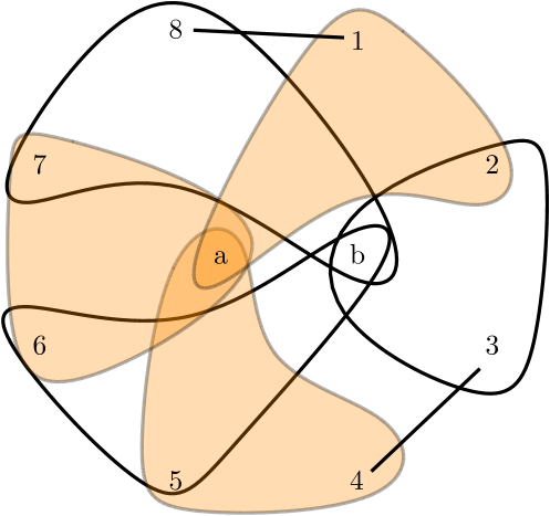
(a) Hypergraph $H_{2}$ with $\mathit{ghw}(H_{2})=\mathit{shw}(H_{2})=2$ and $\mathit{hw}(H_{2})=3$. Some edges are coloured for visual clarity.

(b) The game tree corresponding to the decomposition in Figure 1(a).

Figure 5. Illustration of why monotone strategies for the IRMG can be as powerful as monotone strategies for the Robber and Marshals Game.

A.2. SHW vs. HW

Figure 6. The hypergraph $H_{3}$ (some edges omitted) with $ghw(H_{3})=\mathit{shw}(H_{3})=3$ and $\mathit{hw}(H_{3})=4$ (adapted from (adlermarshals, )).

We now present an example of a hypergraph with $\mathit{shw}=3$ and $\mathit{hw}=4$. To this end, We consider the hypergraph $H_{3}$ adapted from (adlermarshals, ), defined as follows. Let $G=\{g_{11},g_{12},g_{21},g_{22}\}$, $H=\{h_{11},h_{12},h_{21},h_{22}\}$, and $V=\{0,1,2,3,4,0^{\prime},1^{\prime},2^{\prime},3^{\prime},4^{\prime}\}$. The vertices of $H_{3}$ are the set $H\cup G\cup V$. The edges of $H_{3}$ are

$$E(H_{3})= \{\{w,v\}\mid w\in G\cup H,v\in V\}\,\cup\{\{2,4\},\{2^{\prime},4^{\prime}\}\}\,\cup$$

$$\{\{0,1\},\{1,2\},\{0,3\},\{2,3\}\}\,\cup$$

$$\{\{0^{\prime},1^{\prime}\},\{1^{\prime},2^{\prime}\},\{0^{\prime},3^{\prime}\},\{2^{\prime},3^{\prime}\}\}\,\cup$$

$$\{\{g_{11},g_{12},h_{11},h_{12},4^{\prime}\},\{g_{21},g_{22},h_{21},h_{22},3\},$$

$$\phantom{\{}\{g_{11},g_{21},h_{11},h_{21},4\},\{g_{12},g_{22},h_{12},h_{22},3^{\prime}\}\}$$

The hypergraph is shown in Figure 6 with the edges $\{\{w,v\}\mid w\in G\cup H,v\in V\}$ omitted. We have $\mathit{ghw}(H_{3})=3$ and $\mathit{hw}(H_{3})=4$. We now show that indeed also $\mathit{shw}(H_{3})=3$. A witnessing decomposition is given in Figure 7. Note that, strictly speaking, only $\mathit{mw}(H_{3})=3$ is shown in (adlermarshals, ) and, in general, $\mathit{mw}$ is only a lower bound on $\mathit{ghw}$. However, it is easy to verify that $\mathit{ghw}(H_{3})=3$ holds by inspecting the winning strategy for 3 marshals in (adlermarshals, ). Moreover, the $\mathit{ghw}$-result is, of course, implicit when we show $\mathit{shw}(H_{3})=3$ next. Actually, the bags in the decomposition given in Figure 7 are precisely the $\chi$-labels one would choose in a GHD of width $3$. And the $\lambda$-labels are obtained from the (non-monotone) winning strategy for 3 marshals in (adlermarshals, ).

To prove $\mathit{shw}(H_{3})=3$, it remains to verify that all the bags in Figure 7 are contained in $\mathsf{Soft}_{H_{3},3}$. We see that $G\cup H$ are in all the bags and we, therefore, focus on the remaining part of the bags in our discussion. For the root, this is $\{3,0^{\prime},0\}$. Here, the natural cover $\lambda_{1}$ consists of the two large horizontal edges in Figure 6 together with the edge $\{0,0^{\prime}\}$. The union $\bigcup\lambda_{1}$ contains the additional vertex $4^{\prime}$. As $\lambda_{2}$ of Equation 1 we use the same two large edges plus $\{4^{\prime},2^{\prime}\}$. As above, there is only one $[\lambda_{2}]$-edge component, which contains all vertices but $4^{\prime}$. Note that, in contrast to the previous example, $4^{\prime}$ in fact has high degree, but all of the edges that touch $4^{\prime}$ are inside the separator.

Except for the bag $G\cup H\cup\{2,4\}$, the bags always miss either vertex $4$ or $4^{\prime}$ from the “natural” covers, and the arguments are analogous to the ones above for the root bag. For the remaining bag, we consider the cover $\lambda_{1}$ consisting of the two vertical large edges plus the additional edge $\{2,4\}$. Thus, we have the problematic vertex $3^{\prime}$, which is contained in $\bigcup\lambda_{1}$ but not in the bag. Here, we observe a more complex scenario than before. As $\lambda_{2}$ take the two large horizontal edges plus $\{0^{\prime},1^{\prime}\}$. This splits $H_{3}$ into two $[\lambda_{2}]$-components: one with vertices $G\cup H\cup\{0^{\prime},0,1,2,3,4\}$ and another with vertices $G\cup H\cup\{1^{\prime},2^{\prime},3^{\prime},4^{\prime}\}$. The intersection of $\bigcup\lambda_{1}$ with the first complement will produce the desired bag.

Figure 7. A soft hypertree decomposition of $H_{3}$ with width 3.

Appendix B Further Details on Section 5

B.1. Proof of Lemma 6

Proof.

To avoid expressions of the form $\bigcap\bigcup$, we introduce the following notation: for a set $C$ of edges, we write $V(C)$ to denote the set of all vertices contained in $C$, i.e., $V(C)=\bigcup C$.

The proof proceeds in three steps.

Claim A. For every $i\geq 0$, the elements in $E^{(i)}$ can be represented in the form e ∩( [⋂_e_1 ∈E_1 e_1 ∩⋂_C_1 ∈C_1 V(C_1) ] ∪…∪[⋂_e_m ∈E_m e_m ∩⋂_C_m ∈C_m V(C_m) ] ) for some $m\geq 0$, where $e\in E(H)$, $E_{1},\dots,E_{m}\subseteq E(H)$, and $\mathcal{C}$ is a set of sets of edges, such that every element $C\in\mathcal{C}$ is a $[\lambda]$-component, where $\lambda$ is a set of at most $k$ edges from $E(H)$.

The claim is easily proved by induction on $i$. For the induction begin, we have $E^{(0)}=E(H)$ and every element $e\in E(H)$ clearly admits such a representation, namely by setting $m=0$. For the induction step, we use the induction hypothesis for the elements in $E^{(i)}$, expand the definition of the elements in $\mathsf{Soft}_{H,k}^{i}$ and $E^{(i+1)}$ according to Definition 2, and then simply apply distributivity of $\cup$ and $\cap$.

The above claim implicitly confirms that all elements contained in $E^{(i)}$ are either edges in $E(H)$ or subedges thereof. Let us now ignore for a while the sets $\mathcal{C}$ of sets of components in the above representation of elements in $E^{(i)}$. The next claims essentially state that after $n$ iterations, for the sets $E_{j}$ in the above representation, we may use any non-empty subset $E(H)$ and, after another $n$ iterations, no new elements (assuming all sets $\mathcal{C}_{j}$ to be empty) can be produced.

Claim B. Let $i\geq 0$. Then $E^{(i)}$ contains all possible vertex sets $S$ that can be represented as $S=\bigcap_{e^{\prime}\in E^{\prime}}e^{\prime}$ for some $E^{\prime}\subseteq E(H)$ with $|E^{\prime}|\leq i$.

Again, the claim is easily proved by induction on $i$. In the definition of $\mathsf{Soft}_{H,k}^{i}$, we always choose $\lambda_{1}$ as a singleton subset of $E(H)$ and $\lambda_{2}=\emptyset$. Hence, in particular, after $n$ iterations, we have all possible sets of the form $S=\bigcap_{e^{\prime}\in E^{\prime}}e^{\prime}$ for all possible subsets $E^{\prime}\subseteq E(H)$ at our disposal. This fact will be made use of in the proof of the next claim.

Claim C. Suppose that in the definition of $\mathsf{Soft}_{H,k}^{i}$ in Definition 2, we only allow $\lambda_{2}=\emptyset$, i.e., the only component we can thus construct is $C=E(H)$ and, therefore, $V(C)=V(H)$ holds. Then, for every $i\geq 2n$, we have $E^{(i)}=E^{(i+1)}$.

To prove the claim, we inspect the above representation of elements in $E^{(i)}$, but assuming $V(C)=V(H)$ for every $C$. That is, all elements are of the form e ∩( [⋂_e_1 ∈E_1 e_1 ] ∪…∪[⋂_e_m ∈E_m e_m ] ), for some $m\geq 0$. By Claim B, we know that from $i\geq n$ on, we may choose as set $E_{j}$ any subset of $E(H)$. It is easy to show, by induction on $i$, that we can produce any element of the form $e\cap\Big{(}\big{[}\bigcap_{e_{1}\in E_{1}}e_{1}\big{]}\cup\dots\cup\big{[}\bigcap_{e_{i}\in E_{i}}e_{i}\big{]}\Big{)}$ in $E^{(n+i)}$. Then, to prove Claim C, it suffices to show that choosing $i$ bigger than $n$ does not allow us to produce new subedgdes of $e$. To the contrary, assume that there exists $n^{\prime}>n$ and a set $e^{\prime}=e\cap\Big{(}\big{[}\bigcap_{e^{\prime}_{1}\in E^{\prime}_{1}}e^{\prime}_{1}\big{]}\cup\dots\cup\big{[}\bigcap_{e^{\prime}_{n^{\prime}}\in E^{\prime}_{n^{\prime}}}e^{\prime}_{n^{\prime}}\big{]}\Big{)}$ that cannot be represented as $e^{\prime}=e\cap\Big{(}\big{[}\bigcap_{e_{1}\in E_{1}}e_{1}\big{]}\cup\dots\cup\big{[}\bigcap_{e_{n}\in E_{n}}e_{n}\big{]}\Big{)}$. Moreover, assume that $n^{\prime}$ is minimal with this property. Then we derive a contradiction by inspecting the sequence $s_{1}=e\cap\Big{(}\big{[}\bigcap_{e^{\prime}_{1}\in E^{\prime}_{1}}e^{\prime}_{1}\big{]}\Big{)}$, $s_{2}=e\cap\Big{(}\big{[}\bigcap_{e^{\prime}_{1}\in E^{\prime}_{1}}e^{\prime}_{1}\big{]}\cup\big{[}\bigcap_{e^{\prime}_{2}\in E^{\prime}_{2}}e^{\prime}_{2}\big{]}\Big{)}$, …, $s_{n^{\prime}}=e\cap\Big{(}\big{[}\bigcap_{e^{\prime}_{1}\in E^{\prime}_{1}}e^{\prime}_{1}\big{]}\cup\dots\cup\big{[}\bigcap_{e^{\prime}_{n^{\prime}}\in E^{\prime}_{n^{\prime}}}e^{\prime}_{n^{\prime}}\big{]}\Big{)}$. Clearly, this sequence is monotonically increasing and all elements $s_{j}$ are subedges of $e$. By $n^{\prime}>n\geq|V(H)|$, the sequence cannot be strictly increasing. Hence, there exists $j$, with $s_{j}=s_{j-1}$. But then we can leave $\big{[}\bigcap_{e^{\prime}_{j}\in E^{\prime}_{j}}e^{\prime}_{j}\big{]}$ out from the representation $e^{\prime}=e\cap\Big{(}\big{[}\bigcap_{e^{\prime}_{1}\in E^{\prime}_{1}}e^{\prime}_{1}\big{]}\cup\dots\cup\big{[}\bigcap_{e^{\prime}_{n}\in E^{\prime}_{n}}e^{\prime}_{n}\big{]}\Big{)}$ and still get $e^{\prime}$. This contradicts the minimality of $n^{\prime}$.

Completion of the proof of the lemma. From Claim C it follows that after $2n$ iterations, any new elements can only be obtained via the intersections with sets of the form $\bigcap_{C\in\mathcal{C}}V(C)$, where $\mathcal{C}$ is a set of components. Recall that, according to Definition 2, components are only built w.r.t. sets $\lambda_{2}$ of sets of edges from $E(H)$. Hence, all possible components $C$ are available already in the first iteration. Hence, analogously to Claim B, we can show that after $n$ successive iterations, we can choose any sets $\mathcal{C}_{j}$ with $|\mathcal{C}_{j}|\leq i$ for constructing elements of the form e ∩( [⋂_e_1 ∈E_1 e_1 ∩⋂_C_1 ∈C_1 V(C_1) ] ∪…∪[⋂_e_m ∈E_m e_m ∩⋂_C_m ∈C_m V(C_m) ] ), in $E^{(2n+i)}$. In particular, in $E^{(3n)}$, we get any element of the above form for any possible choice of $\mathcal{C}_{j}$ with $|\mathcal{C}_{j}|\leq n$. Finally, analogously to Claim C, we can show that taking sets $\mathcal{C}_{j}$ with $|\mathcal{C}_{j}|>n$ cannot contribute any new element. Again, we make use of the fact that $n\geq|V(H)|$ and it only makes sense to add an element $C$ to $\mathcal{C}_{j}$ if the intersection with $V(C)$ allows us to delete another vertex from $e$. But we cannot delete more than $n$ vertices. ∎

B.2. Proof of Theorem 7

Proof.

Let $\mathcal{G}=(T,\lambda,\chi)$ be a GHD of width $\mathit{ghw}(H)$ of hypergraph $H$. For a node $u$ in $T$, we write $\lambda_{u}$ and $\chi_{u}$ to denote the $\lambda$-label and $\chi$-label at $u$. It suffices to show that, for some $m\geq 0$, the following property holds: for every node $u$ in $T$ and every $e\in E(H)$ with $e\in\lambda_{u}$, the subedge $e\cap\chi_{u}$ is contained in $E^{(m)}$. Clearly, if this is the case, then every bag $\chi_{u}$ is contained in $\mathsf{Soft}_{H,k}^{m}$, since we can define $\lambda_{1}$ by replacing every $e$ in $\lambda$ by $e\cap\chi_{u}$ and setting $\lambda_{2}=\emptyset$. Then $\mathcal{G}^{\prime}=(T,\chi)$ is a candidate TD of $\mathsf{Soft}_{H,k}^{m}$, and, therefore, we get $\mathit{ghw}(H)=\mathit{shw}^{m}(H)$.

To obtain such an $m$ with $(e\cap\chi_{u})\in E^{(m)}$ for every node $u$ in $T$ and edge $e\in\lambda_{u}$, we recall the following result from (JACM, ), Lemma 5.12: Let $e\in\lambda_{u}$ with $e\not\subseteq\chi_{u}$ for some node $u$ and let $u^{\prime}$ be a node with $e\subseteq\chi_{u^{\prime}}$ (such a node $u^{\prime}$ must exist in a GHD). Moreover, let $u=u_{0},\dots,u_{\ell}=u^{\prime}$ be the path from $u$ to $u^{\prime}$ in $T$. Then the following property holds: $e\cap\chi_{u}=e\cap\big{(}\bigcap_{j=1}^{\ell}\bigcup\lambda_{u_{j}}\big{)}$.

Clearly, for every $j$, the bag $\bigcup\lambda_{u_{j}}$ is in $\mathsf{Soft}_{H,k}$ and, therefore, the subedge $s_{j}=e\cap\bigcup\lambda_{u_{j}}$ of $e$ is in $E^{(1)}$. We claim that, for every $i\geq 1$, it holds that $\big{(}\bigcap_{j=1}^{i}s_{j}\big{)}$ is contained in $E^{(i)}$.

Proof of the claim. We proceed by induction on $i$. For $i=1$, the claim reduces to the property that $s_{1}=e\cap\bigcup\lambda_{u_{1}}$ is in $E^{(1)}$, which we have just established. Now suppose that the claim holds for arbitrary $i\geq 1$. We have to show that $\big{(}\bigcap_{j=1}^{i+1}s_{j}\big{)}$ is contained in $E^{(i+1)}$. On the one hand, we have that every $s_{j}=e\cap\bigcup\lambda_{u_{j}}$ is in $E^{(1)}$ and, therefore, also in $E^{(i)+1}$ and in $\mathsf{Soft}_{H,k}^{i+1}$. On the other hand, by the induction hypothesis, $\big{(}\bigcap_{j=1}^{i}s_{j}\big{)}$ is contained in $E^{(i)}$ and, therefore, also in $\mathsf{Soft}_{H,k}^{i}$. Hence, by Definition 2, $\big{(}\bigcap_{j=1}^{i+1}s_{j}\big{)}$ is contained in $E^{(i+1)}$.

We conclude that, for every node $u$ in $T$ and every edge $e\in\lambda_{u}$, the subedge $e\cap\chi_{u}$ = $e\cap\big{(}\bigcap_{j=1}^{\ell}\bigcup\lambda_{u_{j}}\big{)}$ of $e$ is contained in $\mathsf{Soft}_{H,k}^{p}$, where $p$ is the maximal length of paths in $T$. That is, we have $\chi_{u}=\bigcup\lambda^{\prime}_{u}$, where $\lambda^{\prime}_{u}$ is obtained by replacing every edge $e\in\lambda_{u}$ by the subedge $e\cap\chi_{u}$. Hence, $(T,\chi)$ is a candidate TD of $\mathsf{Soft}_{H,k}^{p}$ and, therefore, $\mathit{shw}^{p}(H)=\mathit{ghw}(H)$ ∎

B.3. Proof of Theorem 9

Proof.

Let $(H,\alpha,\beta)$ be the switch graph from Example $2$ of (adlermarshals, ). For convenience we recall the definition here. Let $n\geq 2$. Let $N_{1}$ be a punctured hypergraph with $\mathrm{mw}(N_{1})=\mathrm{mon\text{-}mw}(N_{1})>n$. Let $N_{2}$ be a disjoint copy of $N_{1}$. Let $(H,\alpha,\beta)$ be the switch graph with

$$V(H):=V(N_{1})\cupdot V(N_{2})\cupdot\{m^{\prime}\}\cupdot\{e_{1i}\mid i=1,\ldots,n+1\}\cupdot\{e_{2i}\mid i=1,\ldots,n+1\}.$$

and

(2) $$E(H):= E(N_{1})\cupdot E(N_{2})\cupdot\{\{e_{1i}\}\mid i=1,\ldots,n+1\}\cupdot\{\{e_{2i}\}\mid i=1,\ldots,n+1\}\cupdot\{\{m\}\}$$

(3) $$\cupdot\{\{e_{1i},n_{1}\}\mid i=1,\ldots,n+1,n_{1}\in V(N_{1})\}\cupdot\{\{e_{2i},n_{2}\}\mid i=1,\ldots,n+1mn_{2}\in V(N_{2})\}$$

(4) $$\cupdot\{\{m^{\prime},n\}\mid n\in V(N_{1})\cup V(N_{2})\}.$$

and

$$\alpha=\{\{e_{11}\},\ldots,\{e_{1,n+1}\},\{m^{\prime}\}\}\cup V(N_{2}),$$

$$\beta=\{\{e_{21}\},\ldots,\{e_{2,n+1}\},\{m^{\prime}\}\}\cup V(N_{1}).$$

Let $s:=|V(N_{1})|+(n+1)+1=|\alpha|=|\beta|$.

Let $H_{BOG}$ be the hypergraphs with $n$-machinists associated to $(H,\alpha,\beta)$ as in the proof of Theorem 4.2 in (adlermarshals, ). Let $E(N_{1})$ and $E(N_{2})$ be the sets of edges that are fully contained within $V(N_{1})$ and $V(N_{2})$, respectively. Furthermore, let $E^{+}(N_{1})=E(N_{1})\cup\{\{m^{\prime},n\}\mid n\in N_{1}\}$, and analogously for $E^{+}(N_{2})$. It is known that $\mathit{ghw}(H_{BOG})=s+1$ and $\mathit{hw}(H_{BOG})=s+n+1$ (adlermarshals, ).

We make a critical modification to the construction $H_{BOG}$. Add the new vertex $\star$, and the edges $\{\star,g\}$ for every $g\in B$. That is, $\star$ is adjacent exactly to the balloon vertices. We denote the result of this construction as $H_{BOG}^{\star}$. We will argue the following.

Theorem 1.

$$\mathit{shw}^{1}(H^{\star}_{BOG})=\mathit{ghw}(H_{BOG})\leq\mathit{hw}(H_{BOG})-n=\mathit{hw}(H_{BOG}^{\star})$$

The inequality is an implicit consequence of the construction for Theorem 4.2 in (adlermarshals, ) (and can be validated also through our argument). Furthermore $H_{BOG}$ is an induced subhypergraph of $H^{\star}_{BOG}$ (induced on all vertices but $\star$). It is easy to see that hypertreewidth is monotone over induced subhypergraphs, thus $\mathit{hw}(H_{BOG})\leq\mathit{hw}(H^{\star}_{BOG})$. To show the equality we explicitly give a (CompNF) tree decomposition for $H^{\star}_{BOG}$ using only bags from $\mathsf{Soft}^{1}_{H^{\star}_{BOG},s+1}$ in Figure 8. We verify this through a number of independent claims.

Claim. The TD from Figure 8 is a valid tree decomposition.

It is straightforward to check that every edge of $H^{\star}_{BOG}$ is covered. To cover the eyelet edges some care is required to maintain connectedness. Recall that the eyelet edges are for every $g\in B,h\in E(H)$ and $\ell\in[m]$ (where $m$ is an integer, unrelated to the vertex $m^{\prime}$ in the switch graph.) there are edges $\{g,p_{\ell}(g,h)\}$ and $h\cup\{p_{\ell}(g,h)\}$. Observe that the edges $E(H)$ can be partitioned into $E^{+}(N_{1})$, $E^{+}(N_{2})$ as well as the sets of edges connecting every $e_{1i}$ to all vertices in $N_{1}$ and $e_{2i}$ to all vertices in $N_{2}$. With this partition in mind one can then observe that the decomposition in Figure 8 satisfies the connectedness condition. $\blacktriangle$

Claim. $\{\star\}\cup B\in\mathsf{Soft}^{0}_{H^{\star}_{BOG},s+1}$.

Take as $\lambda_{2}$ in Equation 1 the edges $\{a_{1},\dots,a_{s}\}$. We have $\bigcup\lambda_{2}\supset B$ (cf., (adlermarshals, )). Then, $\star$ is not $[\lambda_{2}]$-connected to any other vertex. Hence there is a $[\lambda_{2}]$-component $C$ where $\bigcup C$ equals $\star$ plus all adjacent vertices to $\star$. By definition then $\bigcup C=\{star\}\cup B$. $\blacktriangle$

Claim. For every $i$, the subedges $a^{\prime}_{i}=\{g_{i1},\dots,g_{is}\}$ and $b^{\prime}_{j}=\{g_{1j},\dots,g_{sj}\}$ are in $E^{(1)}$.

We argue for $a^{\prime}_{i}$, the case for $b^{\prime}_{j}$ is symmetric. Recall from the construction of $H_{BOG}$ that there is an edge $a_{i}=\{g_{i1},\dots,g_{is}\}\cup\alpha_{i}$ for every $i\in[s]$. Thus $a_{i}\in E^{(0)}$, and from the previous claim $\{\star\}\cup B\in\mathsf{Soft}^{0}_{H^{\star}_{BOG},s+1}$. Hence $a^{\prime}_{i}\in E^{(0)}\mathop{\raisebox{0.86108pt}{\ooalign{$\bigcap$\cr\hskip 1.13809pt\raisebox{-0.56905pt}{${\times}$}}}}\mathsf{Soft}^{0}_{H^{\star}_{BOG},s+1}=E^{(1)}$ $\blacktriangle$

Claim. For every $i\in[n+1]$, $B\cup V(N_{2})$ is the union of $s$ edges in $E^{(1)}$. The same holds also for $B\cup V(N_{1})$.

The respective edges are $X=\{a^{\prime}_{1},\dots,a^{\prime}_{n+2},a_{n+3},\dots,a_{s}\}$. That is we take the subedges of $a_{i}$ for the first $n+2$ indexes, i.e., those indexes where $\alpha_{i}=e_{1i}$ or $\alpha_{i}=m$. The $\alpha$ for the rest of the indexes make up exactly the set $V(N_{1})$ by definition. In summary we have $\bigcup X=\left(\bigcup_{i=1}^{s}a_{i}\right)\setminus\{e_{11},\dots,e_{1,n+1},m^{\prime}\}=B\cup V(N_{2})$. For the case with $V(N_{1})$ make the same construction for the $b_{j}$ edges. $\blacktriangle$

Claim. The TD from Figure 8 uses only bags from $\mathsf{Soft}_{H^{\star}_{BOG},s+1}$.

There are 4 kinds of bags that are not simply unions of $s+1$ (even 2) edges. All are either of the form $X=V(N_{2})\cup B\cup\{v\}$ or, $Y=V(N_{1})\cup B\cup\{v\}$. From the previous claim it then follows immediately that these are in $\mathsf{Soft}_{H^{\star}_{BOG},s+1}$. $\blacktriangle$

Figure 8. A soft hypertree decomposition of width $s+1$ for $H^{\star}_{BOG}$. We note that the terms $\ell\in[m]$ refer to the number $m$ of eyelet vertices from the construction of $H_{BOG}$ in (adlermarshals, ). For consistency we minimised changes in the naming from the reference, despite the slightly confusing similarity to $m^{\prime}$ (also called $m$ in (adlermarshals, )), a vertex in the switch graphs that the construction is applied to.

The results in (adlermarshals, ) are stated in terms of games, in particular showing that the gap between marshall width $mw$ and monotone marshall width $mon$-$mw$ on $H_{BOG}$ is at least $n$. It has been considered folklore that this implies also that the gap between $\mathit{ghw}$ and $\mathit{hw}$ is at least $n$ on these gaps (and thus arbitrarily high in general). But to the best of our knowledge no proof of this is explicitly written down in the literature. The problem being, that while $mon$-$mw(H)=\mathit{hw}(H)$, the marshall width itself is not necessarily equal to $\mathit{ghw}$ but only a lower bound. We note that Figure 8 is also a generalised hypertree decomposition of width $s+1$, and also serves to fill in this small gap in the literature. ∎

Appendix C Further Details on the Implementation

This section is meant to give full technical details on the tools that we used and implemented to perform the experiments. It will also detail the cost functions, which extract statistics from the database to assign a cost estimate to a CTD, where a lower value indicates lower estimated runtime. As was mentioned in Section 7, our tools are based on existing work published in (bohm2024rewrite, ; DBLP:journals/corr/abs-2303-02723, ). Our source code is available anonymously: https://anonymous.4open.science/r/softhw-pods25.

C.1. Implementation Overview

Our system evaluates SQL queries over a database, but does so by way of first finding an optimal decomposition, then using the decomposition to produce a rewriting - a series of SQL queries which together produce the semantically equivalent result as the input query – and then runs this rewriting on the target DBMS. This procedure is meant to guide the DBMS by exploiting the structure present in the optimal decomposition. A graphical overview of the system is given in Figure 9. For simplicity, we assume here that only Postgres is used.

The system consists of two major components – a Python library providing an interface to the user, which handles the search for the best decompositions, and a Scala component which connects to the DBMS and makes use of Apache Calcite to parse the SQL query and extract its hypergraph structure, as well as extracing from the DBMS node cost information (which we will detail further below) and generate the rewritings.

The Python library – referred to as QueryRewriterPython – acts as a proxy to the DBMS, and is thus initialised like a standard DBMS connection. The library is capable of returning not just the optimal rewriting, but can provide the top-$n$ best rewritings, as reported on in LABEL:app:expdetails. As seen in Figure 9, on start up QueryRewriterPython starts QueryRewriterScala as a sub-process. QueryRewriterPython communicates with it via RPC calls using Py4J. QueryRewriterScala obtains the JDBC connection details from QueryRewriterPython, and connects to the DBMS using Apache Calcite, in order to be able to access the schema information required later. The input SQL query is then passed to QueryRewriterScala. Using Apache Calcite, and the schema information from the database, the input SQL query is parsed and converted into a logical query plan. After applying simple optimiser rules in order to obtain a convenient representation, the join structure of the plan is extracted and used to construct a hypergraph. Subtrees in the logical representation of the query, which are the inputs to joins, such as table scans followed by projection and filters, are kept track of, and form the hyperedges of this hypergraph. Later, when creating the rewriting, the corresponding SQL queries for these subtrees is used in the generation of the leaf node VIEW expressions. After retrieving the hypergraph, the QueryRewriterPython enumerates the possible covers, i.e., hypertree nodes, whose size is based on the width parameter $k$. The list of nodes is sent to the QueryRewriterScala, where the costs of each of these nodes are estimated. We will detail the two used cost functions in the next subsection. Once all the cost functions have been computed, the QueryRewriterPython follows an algorithm in the vein of Algorithm 2, in order to find the best or the top-$n$ best decompositions. Finally, the decompositions are passed to the QueryRewriterScala in order to generate the rewritings.

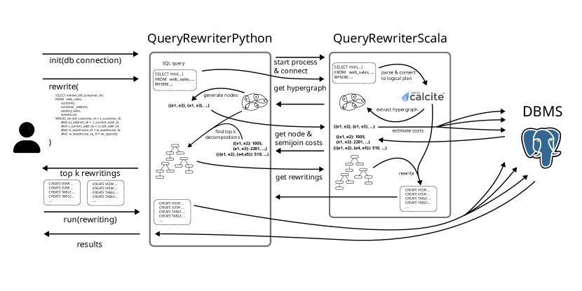
Figure 9. Overview of the components of the query rewriting system

C.2. Cost Functions for Section 7

In this section we provide full details for the cost functions implemented for our optimisation experiments in Section 7.

C.2.1. A Cost Function Based on DBMS-Estimates

To estimate the costs of the decompositions, we make use of Postgres’ cost estimates, as they are internally used by the system for finding a good query plan. Postgres estimates the costs of a query plan in abstract units based on assumptions about lower-level costs in the system, such as disk I/O, or CPU operations. By making use of EXPLAIN statements, it is possible to retrieve the total cost of a plan estimated by the DBMS.

When estimating the costs of bags in the decomposition, we construct the join query corresponding to the bag, and let Postgres estimate the cost of this query in an EXPLAIN statement.

(5) $$\mathit{cost}(u):=\begin{cases}C(\pi_{B_{u}}(R_{1}\bowtie R_{2}\bowtie\cdots\bowtie R_{n}))&\text{if }n>1\\ 0&\text{if }n=1\end{cases}$$

where $C(q)$ corresponds to the costs estimated by Postgres for the query $q$.

To estimate the costs of a subtree, we also consider the costs of computing the bottom-up semijoins. Because Postgres includes the costs of scanning the relations which are semijoined, and any joins inside the bags, in the total costs, we have to subtract these costs from the semijoin-costs. Due to noisy estimates, we have to avoid the total cost becoming negative, and thus set a minimum cost.

(6) $$\mathit{cost}(T_{p}):=\mathit{cost}(p)+\sum_{i=1}^{k}\left(\mathit{cost}(T_{c_{i}})+min(C(J_{p}\ltimes J_{c_{i}})-C(J_{p})-C(J_{c_{i}}),1)\right)$$

C.2.2. A Cost Function Based on Actual Cardinalities

Because we observe problematic unreliability of cost estimates from the DBMS, we also consider an idealised cost function, that is omniscient about bag sizes and uses these to estimate cost of individual operations. This has the weakness of not taking physical information, such as whether relations are already in memory (or even fit wholly in memory) or specific implementation behaviour (which we surprisingly observe to be highly relevant in our experiments). Nonetheless, we find it instructive to compare these costs to the estimate based cost function to correct for cases where estimates are wildly inaccurate.

First, the cost for bags. We will assume we know the cardinality of the bag (simulating a good query planner) and combine this with the size of the relations that make up the join. The idea is simple, to compute the join we need to at least scan every relation that makes up the join (that is, linear effort in the size of the relations). And then we also need to create the new relation, which takes effort linear in the size of the join result. We thus get for a node $u$ of a decomposition, whose bag is created by cover $R_{1},\dots,R_{n}$:

(7) $$\mathit{cost}(u):=\begin{cases}|J_{u}|+|\sum_{i=1}^{n}|R_{i}|\cdot\log|R_{i}|&\text{if }n>1\\ 0&\text{if }n=1\end{cases}$$

where $J_{u}=\pi_{B_{u}}(R_{1}\bowtie R_{2}\bowtie\cdots\bowtie R_{n})$, i.e., table for the node.

The cost for a subtree then builds on this together with some estimate of how effective the semi-joins from the subtrees will be. We will estimate this very simply, by seeing how many non primary-key attributes of the parent appear in a subtree. The point being that if something is a FK in the parent, we assume that every semi-join will do nothing. If something is not a PK/FK relationship in this direction, then we assume some multiplicative reduction in tuples for each such attribute. For every node $p$ in a rooted decomposition we thus define $\mathit{ReduceAttrs}(p)$ as the set containing every attribute $A$ in $B_{p}$, for which $A$ appears in a subtree rooted at a child of $p$, where it does not come from a relation where $A$ is the primary key.

With this in hand we then estimate the size of the node after the up-phase semi-joins have reached it:

(8) $$\mathit{ReducedSz(u)}:=\begin{cases}0&\text{if }ReducedSz(c)=0\text{ for any child $c$ of $u$}\\ \frac{|J_{u}|}{1+|\mathit{ReduceAttrs(u)}|}&\text{otherwise}\end{cases}$$

Importantly, if relation $C$ is empty, PostgreSQL never scans $U$ in the semi-join $U\ltimes C$, to capture this define the following for nodes $u$. ScanCost(u) := {