BA-BFL: Barycentric Aggregation for Bayesian Federated Learning

Abstract

In this work, we study the problem of aggregation in the context of Bayesian Federated Learning (BFL). Using an information geometric perspective, we interpret the BFL aggregation step as finding the barycenter of the trained posteriors for a pre-specified divergence metric. We study the barycenter problem for the parametric family of $\alpha$-divergences and, focusing on the standard case of independent and Gaussian distributed parameters, we recover the closed-form solution of the reverse Kullback–Leibler barycenter and develop the analytical form of the squared Wasserstein-2 barycenter. Considering a non-IID setup, where clients possess heterogeneous data, we analyze the performance of the developed algorithms against state-of-the-art (SOTA) Bayesian aggregation methods in terms of accuracy, uncertainty quantification (UQ), model calibration (MC), and fairness. Finally, we extend our analysis to the framework of Hybrid Bayesian Deep Learning (HBDL), where we study how the number of Bayesian layers in the architecture impacts the considered performance metrics. Our experimental results show that the proposed methodology presents comparable performance with the SOTA while offering a geometric interpretation of the aggregation phase.

1 Introduction

Federated Learning (FL) is considered a de facto standard in decentralized learning systems where strong privacy guarantees are required. As envisioned in [1], an FL system is comprised of a server, storing a global model, which interfaces with multiple clients, i.e., end-devices, possessing private data. FL schemes mainly operate in two phases: a learning phase, where each client trains its local model on the locally available data, and an aggregation phase, where the local models are sent to the server and “merged” according to a pre-determined rule. The two phases alternate iteratively, using the global model resulting from the previous iteration as updated local models in the current one.

Aggregation is a key operation for combining individual contributions into a global model while keeping data secure and being communication efficient. Although different aggregation techniques are proposed in the literature, e.g., [2], most known aggregation methods rely on variations of weighted averaging. For example, FedAVG [1] and FedProx [3] aggregate the local model through the weighted average of their parameters. The weights become an important design parameter, encoding auxiliary attributes such as the importance of the local models for the objective of the algorithm or proportionally to the volume of data held by each client.

One key challenge in FL, and generally in distributed learning systems, is the statistical heterogeneity of the involved clients. In most realistic scenarios, the datasets available to each end-user rarely satisfy the ideal IID conditions, showing heterogeneous properties, i.e., shifts, across the clients. Commonly observed shifts are surveyed in [4, 3], where five major models of heterogeneity are identified: label distribution skew, i.e., variance in the number of samples representative of a specific label across users (under or over-represented classes); feature distribution skew, i.e., features associated with a class label vary across users; concept drift, i.e., different clients have the same labels for different features; concept shift, i.e., different clients may have mismatched labels for the same samples; quantity skew, i.e., heterogeneity in the size of the datasets possessed by each client. Although compelling from the practical point of view, approaching all the listed non-idealities may not be feasible. Therefore, the vast majority of the literature considers only subsets of them [5, 6, 7].

Clients’ heterogeneity also raises other issues in the distributed architecture, such as the problem of algorithmic fairness. Algorithmic fairness refers to treating all individuals or groups impartially in decision-making, without bias or favoritism based on their innate or acquired characteristics [8, 9]. In the context of FL, models are trained on data from multiple sources, which may represent diverse populations. Neglecting the fairness aspects could potentially lead to introducing or reinforcing existing biases in the global model, leading to unfair treatment of certain groups. Multiple works focused their attention on fairness in FL algorithms, suggesting solutions such as Personalized FL. A taxonomy of Fairness-Aware FL approaches that encompass key phases in FL such as client selection, optimization, contribution assessment, and incentive distribution can be found in [10].

Building on the applicability of FL in real-world scenarios, uncertainty quantification (UQ) and model calibration (MC) are central qualities of reliable models. Nonetheless, these aspects have not been investigated thoroughly in the existing research around deterministic FL. A preliminary study on the topic, with specific application to healthcare, is provided in [11], through an overview of various UQ methods in the deterministic FL setting, later implemented also in [12]. We stress, however, that the surveyed techniques are mainly inspired by Bayesian-like solutions, such as Bayesian ensembles and Monte Carlo dropout.

Improving the reliability of models is where Bayesian Learning (BL) excels, as Bayesian methods allow for better quantification of the model uncertainty and calibration, rendering it a compelling solution for FL in the non-IID context. FedPPD [13] introduces an FL framework that incorporates UQ, where each client, in each round, estimates the posterior distribution over its parameters and the posterior predictive distribution (PPD). The PPD is then distilled into a single deep neural network and sent to the server. pFedBayes [14] and Fedpop [15] are also Bayesian approaches with a focus on UQ aspects, proposed in the context of personalized BFL. Nonetheless, we emphasize that many of the existing methods [13, 14, 16, 17] rely on variations of weighted averaging of the posteriors’ parameters.

Contributions

This work aims to introduce novel aggregation methodologies in the context of BFL leveraging barycentric aggregation (BA-BFL). Given a divergence metric, we interpret the aggregation process as a geometric problem, where the global model is identified as the barycenter of the local posteriors. In light of this perspective, we study the barycenter problem for the parametric family of $\alpha$-divergences for general distributions. Subsequently, considering the specific case of independent and Gaussian distributed posteriors, we recover the analytical barycenter solution for the reverse-Kullback-Leiber (RKL) divergence and derive a closed-form solution for the squared Wasserstein-2 ($\operatorname*{W_{2}^{2}}2$) barycenter, through which we define the RKLB and WB aggregation methodologies. We compare the performance of the proposed techniques against SOTA Bayesian aggregation methods in terms of accuracy and UQ scores within a heterogeneous setting. To address the gap identified in the BFL literature and following the analysis of Hybrid Bayesian Deep Learning (HBDL) envisioned in [18], we extend our study to analyze the performance impact of considering only a limited number of Bayesian layers on the different Bayesian aggregation techniques. Furthermore, this paper takes a step towards analyzing BFL aggregation methods, including the novel approach we propose, from a fairness perspective. To the best of our knowledge, this has not been addressed in the existing FL literature.

2 Background and Related Work

Federated Learning

An FL system [1] consists of a central server and $N$ clients, engaging in an iterative learning process involving server-client communication. For each communication round, the $k^{th}$ client trains its local model, parameterized by $\theta_{k}$, on its private data $\mathcal{D}_{k}$. Subsequently, the model parameters $\theta_{k}$ are sent to the server, which aggregates all the clients’ models to obtain the global model, later sent to the clients to refine their local models for the next communication round. By aggregating the local models of the clients, FL seeks to achieve a global model $\theta^{*}$ on $\mathcal{D}=\bigcup_{k=1}^{N}\mathcal{D}_{k}$, the aggregated dataset from all participating clients.

In general, an FL system considers objective functions of the form

$$\min_{{\theta}}F({\theta})=\sum_{k=1}^{N}w_{k}F_{k}({\theta})$$ (1)

where $F_{k}({\theta})=\mathbb{E}_{(x,y)\sim\mathcal{D}_{k}}[\mathcal{L}(\theta;(x,y)]$ is the local objective function of the $k^{th}$ client and $w_{k}$ is its associated weight such that $\sum_{k=1}^{N}w_{k}=1$. Minimizing $F_{k}(\theta)$ at each communication round gives rise locally to $\theta_{k}$.

Fairness

The topic of fairness intersects multiple domains, including social sciences, law, machine learning, and statistics, each leading to different perspectives and implicitly different definitions. [8] provides an overview of the most significant aspects of fairness in the context of ML and categorizes them into individual fairness, where the goal is to achieve comparable predictions for similar individuals, group fairness, ensuring that all groups receive equal treatment, and subgroup fairness, which aims to capture the most beneficial aspects of both group-based and individual-based approaches to fairness.

In FL, we consider not only the fairness of each individual ML model but also the fairness of the algorithm across different clients within the FL setting. To enhance clients’ engagement, it is important to ensure that the FL algorithm does not discriminate against certain clients. Thus, we regard fairness from a sociological point of view where the two main definitions are:

• Utilitarianism [19] is a notion of social science where as long as the overall performance of the whole society is optimal, we call the society to be fair. In FL, this results in looking at the average performance of all the users.

• Egalitarianism [20, 21] is a fairness rule aiming to maximize the worst-case performance.

In [22], the authors explored proportional fairness in FL and propose PropFair as a proportional fair FL algorithm, achieving a good balance between utilitarian and egalitarian fairness.

Hybrid Bayesian Deep Learning (HBDL)

Despite the remarkable results in terms of model performance, Deep Learning (DL) does not address crucial problems in realistic scenarios, such as reliability and UQ. In a recent position paper [23], the authors propose Bayesian Deep Learning (BDL) as a solution for the ethical, privacy, and safety challenges of modern DL. Acknowledging ongoing issues with BDL, e.g., the added complexity cost of performing BL on large-scale deep models, the authors envision the alternative framework of HBDL to maintain the efficiency and lower complexity of DL while retaining the reliability of BDL. HBDL is also discussed in [24] as Bayesian inference on the (n-)last layer(s) only. The idea behind this framework is to substitute part of the layers in a Bayesian deep model with deterministic layers, making them equivalent to the classical DL counterpart. The possibility of having only a partially Bayesian model allows for retaining UQ capabilities while reducing the complexity compared to a fully Bayesian model.

Bayesian Federated Learning

FL naturally inherits the issues of DL we discussed so far, as well as some of the highlighted solutions. BFL aims to integrate BDL strengths into FL. [25] presents a taxonomy of BFL, categorizing it following the Bayesian perspective into:

• Client-side BFL [26, 14, 27, 28, 16, 29, 30, 13], where Bayesian neural networks and Bayesian optimization are employed to train the local models.

• Server-side BFL [31, 32, 33, 34], where Bayesian techniques like Bayesian model ensembling or Bayesian posterior decomposition are used to aggregate the local models in order to obtain the global model.

Divergence metrics and Information Geometry

Dealing with the set of local posteriors generated by the clients, BFL requires a principled way to compare and aggregate the received distributions. The majority of the proposed solutions consider parameterized local statistical models, later aggregated through operations in the shared parameter space. However, following the solutions proposed in FL, these methods often assume an Euclidean structure in the parameter space, proposing aggregation relying on simple averaging of the local parameters, disregarding the implications on the underlying manifold to which the posterior probabilities belong.

Given a statistical manifold $\mathcal{M}$, a divergence $D:\mathcal{M}\times\mathcal{M}\to[0,+\infty)$ is a non-negative function expressing the degree of dissimilarity between two distributions on $\mathcal{M}$. Widely used in statistics and ML, some examples include:

• the parametric family of $\alpha$-divergences [35], defined for $\alpha\in\mathbb{R}\setminus\{0,1\}$ as

  $$D_{\alpha}(p\|q)\triangleq\frac{1}{\alpha(1-\alpha)}\left(1-\int p_{\nu}^{\alpha}q_{\nu}^{1-\alpha}d\nu\right),$$

  where $p_{\nu}=\frac{dp}{d\nu}$ and $q_{\nu}=\frac{dq}{d\nu}$ are the Radon-Nicodym derivatives w.r.t. a reference measure $\nu$. This parametric family includes several commonly used divergences, obtained for specific values of $\alpha$, e.g., for $\alpha=1/2$ we obtain the Hellinger distance $H(p||q)$, for $\alpha\to 1$ we have the KL divergence $D_{KL}(p||q)$, for $\alpha\to 0$ we obtain the RKL divergence $\operatorname*{D_{RKL}}(p||q)=D_{KL}(q||p)$.

• the squared Wasserstein-2 distance $\operatorname*{W_{2}^{2}}2$, introduced in [36] and defined as

  $$\operatorname*{W_{2}^{2}}2(p,q)\triangleq\min_{\pi\in\Pi}\mathbb{E}_{\pi}\left[||X-Y||^{2}\right],$$

  where $(X,Y)\sim\pi$ and $\Pi$ is the set of all distributions $\pi$ such that its marginal distributions are $p$ and $q$.

Information Geometry [37] studies the geometric properties that a divergence function induces on a manifold, allowing translation of operations naturally defined on a manifold, such as projections onto sets [38, 39], or identifying centers of mass of a set of points, i.e., barycenters [40, 41], to operations on the parameter space. We leverage this connection to derive aggregation methodologies for the local models in the parameter space as interpretable operations on the manifold.

3 Proposed Method

In this section, we present our main theoretical results. We start by formalizing the essential technical aspects of the Client-side BFL framework.

Client-Side BFL

The Bayesian view presents a different framework for FL. The goal is to estimate the posterior distribution of the global model’s parameters, $p(\theta^{*}|\mathcal{D})$, given the posterior distributions of local models $p(\theta_{k}|\mathcal{D}_{k})$.

Nevertheless, exact posterior inference is usually intractable, requiring the use of approximate inference methods instead. In this work, we consider Variational Inference [42, 43] to approximate the local posteriors given a common prior distribution $p(\theta)$ and the client likelihoods $p(\mathcal{D}_{k}|\theta_{k})$.

For a parametric family $\mathcal{Q}$, the optimization problem seeks to identify the distribution $q\in\mathcal{Q}$ that minimizes the KL divergence from the posterior distribution $p(\theta|\mathcal{D})$, i.e.,

$$\min_{q(\theta)\in\mathcal{Q}}\operatorname*{D_{KL}}(q(\theta)\|p(\theta|\mathcal{D}))$$ (2)

However, the minimization in (2) is not directly tractable and is commonly approached through the derivation of the Negative Evidence Lower BOund (NELBO) surrogate objective

$$\min_{q(\theta)\in\mathcal{Q}}-\mathbb{E}_{q(\theta)}[\log p(\mathcal{D}|\theta)]+\operatorname*{D_{KL}}(q(\theta)||p(\theta)).$$ (3)

The local models are trained by minimizing (3) to achieve their models’ posterior distributions $p(\theta_{k}|\mathcal{D}_{k}),~{}\forall k\in\{1,..,N\}$. The local posteriors are then aggregated in order to get the global model’s posterior $p(\theta^{*}|\mathcal{D})$. Given this setting, we now introduce our main assumptions regarding the common prior $p(\theta)$ and the parametric family $\mathcal{Q}$, which will stay valid throughout the rest of this paper.

Assumption 1.

For each client, we assume the prior distribution $p(\theta)$ to be a $d$-dimensional Gaussian with independent marginals, parameterized by a zero mean vector $\mathbf{0}_{d}$ and an identity covariance matrix $\mathbf{I}_{d}$.

Assumption 2.

(Mean-field Model) The parametric family $\mathcal{Q}$ is composed of $d$-dimensional Gaussian distributions with independent marginals, i.e., $\theta\sim\mathcal{N}(\mu,\Sigma)$, with mean $\mu\in\mathbb{R}^{d}$ and diagonal covariance $\Sigma=\operatorname*{diag}(\sigma^{2}_{1},\ldots,\sigma^{2}_{d})$.

Bayesian Aggregation as Posteriors Barycenter

The main novelty of this work stands in the introduction of Barycentric Aggregation for BFL (BA-BFL), an aggregation method inspired by the geometric properties of the manifold to which the local posteriors $\{p(\theta_{k}|\mathcal{D}_{k})\}_{k=1\ldots N}$ belong. Given a divergence metric $D$, we propose as a global model the barycenter $p^{*}_{D}$ of the set of clients’ posteriors, i.e., the distribution that minimizes the weighted divergence from a given set. The following problem formalizes this interpretation of the aggregation process.

Problem 1.

($D$-barycenter) Given a statistical manifold $\mathcal{M}$, a divergence function $D:\mathcal{M}\times\mathcal{M}\to[0,\infty)$, and a set of distributions $\mathcal{S}=\{p_{k}\}_{k=1\ldots N}\subseteq\mathcal{M}$ with associated normalized weights $\{w_{k}\}_{k=1\ldots N}$, i.e., $\sum_{k=1}^{N}w_{k}=1$, the barycenter $p^{*}_{D}$ of the set $\mathcal{S}$ is defined as:

$$p^{*}_{D}=\operatorname*{arg\,min}_{q\in\mathcal{M}}\sum_{k=1}^{N}w_{k}D(p_{k}||q).$$ (4)

We now study Problem 1 under various assumptions on the distribution set $\mathcal{S}$ and divergence metric $D$. First, we consider the generic case where $D=D_{\alpha}$, namely, it belongs to the family of $\alpha$-divergences, without any additional assumption on the set $\mathcal{S}$.

Theorem 1.

($\alpha$-barycenter) Let $D(p||q)=D_{\alpha}(p||q)$ with $\alpha\in\mathbb{R}\setminus\{0\}$. Then, the barycenter $p^{*}_{D_{\alpha}}$ in (4) is the following:

$$p^{*}_{D_{\alpha}}=\frac{\left(\sum_{k=1}^{N}w_{k}p_{k}^{\alpha}\right)^{\frac{1}{\alpha}}}{\bigints\left(\sum_{k=1}^{N}w_{k}p_{k}^{\alpha}\right)^{\frac{1}{\alpha}}d\nu}.$$ (5)

Additionally, for $\lim_{\alpha\to 0}D_{\alpha}(p||q)=D_{RKL}(p||q)$, the barycenter $p^{*}_{RKL}$ in (4) becomes:

$$p^{*}_{RKL}=\frac{\prod_{k=1}^{N}p_{k}^{w_{k}}}{\bigints\prod_{k=1}^{N}p_{k}^{w_{k}}d\nu}.$$ (6)

Proof.

Let the distribution $\hat{p}$ be defined as:

$$\hat{p}\triangleq c\cdot\left(\sum_{k=1}^{N}w_{k}p_{k}^{\alpha}\right)^{\frac{1}{\alpha}}\text{where}~{}c=\frac{1}{\bigints\left(\sum_{k=1}^{N}w_{k}p_{k}^{\alpha}\right)^{\frac{1}{\alpha}}d\nu}.$$

Then, the right-hand side of $\eqref{eq:barycenter1}$ can be expressed as:

$$\sum_{k=1}^{N} w_{k}D_{\alpha}(p_{k}||q)$$

$$=\sum_{k=1}^{N}w_{k}\left[\frac{1}{\alpha(1-\alpha)}\left(1-\int q^{1-\alpha}p_{k}^{\alpha}d\nu\right)\right]$$

$$=\frac{1}{\alpha(1-\alpha)}\left[1-\int q^{1-\alpha}\left(\sum_{k=1}^{N}w_{k}p_{k}^{\alpha}\right)d\nu\right]$$

$$=\frac{1}{\alpha(1-\alpha)}\left[1-\int q^{1-\alpha}\frac{\hat{p}^{\alpha}}{c^{\alpha}}d\nu\right]$$

$$=\frac{1}{\alpha(1-\alpha)}\left[1-\frac{1}{c^{\alpha}}+\frac{1}{c^{\alpha}}-\int q^{1-\alpha}\frac{\hat{p}^{\alpha}}{c^{\alpha}}d\nu\right]$$

$$=\frac{1-c^{-\alpha}}{\alpha(1-\alpha)}+\frac{c^{-\alpha}}{\alpha(1-\alpha)}\left[1-\int q^{1-\alpha}{\hat{p}^{\alpha}}d\nu\right]$$

$$=\frac{1-c^{-\alpha}}{\alpha(1-\alpha)}+c^{-\alpha}D_{\alpha}(\hat{p}||q).$$ (7)

Since (7) depends on $q$ only through the term $D_{\alpha}(\hat{p}||q)$, the minimum in $\eqref{eq:barycenter1}$ is attained by $q=\hat{p}$ due to the fundamental properties of divergence measures, i.e., $D(\hat{p}||q)\iff q=\hat{p}$, proving the first part of the theorem. The second part can be obtained following similar steps, and by considering that $\lim_{\alpha\to 0}D_{\alpha}(p||q)=\operatorname*{D_{RKL}}(p||q)$. This concludes the proof. ∎

We now focus on the case where all $p_{k}\in\mathcal{S}$ are $d$-dimensional Gaussian distributions, i.e., $p_{k}=\operatorname*{\mathcal{N}}(\mu_{k},\Sigma_{k})$, with mean $\mu_{k}$ and covariance matrix $\Sigma_{k}$. This setting derives from Assumption 2, where we assume that the parameters of each Bayesian layer are Gaussian distributed. For the same reasons, we are also interested in the cases where the resulting barycenter is itself Gaussian, to enforce that global and local models belong to the same family of distributions. Alas, this is not the case for the majority of $\alpha$-divergences, as discussed in the following remark.

Remark 1.

(On the $\alpha$-barycenter of a set of Gaussians) Given $\mathcal{S}=\{\operatorname*{\mathcal{N}}(\mu_{k},\Sigma_{k}\}_{k=1\ldots N}$, the barycenter distribution $p^{*}_{D_{\alpha}}$ in (5) is not Gaussian. In fact, $(p^{*}_{D_{\alpha}})^{\alpha}\propto\sum_{k=1}^{N}w_{k}p_{k}^{\alpha}$, showing that the resulting barycenter is related to the Gaussian mixture obtained from the weighted sum of the elements of $\mathcal{S}$. On the other hand, $p^{*}_{RKL}$ is still Gaussian since the Gaussian family is closed under the product operation and (6) is the normalized product of unnormalized Gaussians.

In light of the above technical remark, among the considered $\alpha$-divergences we focus exclusively on the case of $\alpha\to 0$, i.e., $p_{RKL}^{*}$, as the barycenter naturally belongs to the Gaussian family, leaving the study of other $\alpha$-divergences as future work. The following corollary specializes (6) for the Gaussian case.

Corollary 1.

(Gaussians $\operatorname*{D_{RKL}}$-barycenter) Let $\mathcal{S}=\{\operatorname*{\mathcal{N}}(\mu_{k},\Sigma_{k})\}_{k=1\ldots N}$ and let $D(p||q)=\operatorname*{D_{RKL}}(p||q)$. Then, the barycenter $p_{D}^{*}\equiv{p}_{RKL}^{*}$ in (4) is Gaussian, i.e, $p_{RKL}^{*}=\operatorname*{\mathcal{N}}(\mu_{RKL},\Sigma_{RKL})$, with parameters:

$$\Sigma_{RKL}=\left(\sum_{k=1}^{N}w_{k}\Sigma_{k}^{-1}\right)^{-1},~{}\mu_{RKL}=\Sigma_{RKL}\sum_{k=1}^{N}w_{k}\Sigma_{k}^{-1}\mu_{k}.$$ (8)

Proof.

This follows from evaluating (6) for the given $\mathcal{S}$. ∎

It should be remarked that the same result as in Corollary 1 was obtained in [44] using different methodologies.

Similarly to the $D_{RKL}$ divergence, the barycenter of a set of Gaussians in the Wasserstein-2 distance belongs to the same family. In the general setting, the parameters of the barycenter are obtained through a set of fixed-point equations [45]. However, to obtain analytic expressions, we consider only the case where the set of covariance matrices $\{\Sigma_{k}\}_{k=1\ldots N}$ is composed of diagonal matrices, i.e., $\Sigma_{k}=\operatorname*{diag}(\sigma^{2}_{k,1},\ldots,\sigma^{2}_{k,d})$. The following theorem reports the resulting closed-form expressions.

Theorem 2.

(Independent Gaussians for $\operatorname*{W_{2}^{2}}2$-barycenter) Let $\mathcal{S}=\{\operatorname*{\mathcal{N}}(\mu_{k},\Sigma_{k})\}_{k=1\ldots N}$ with $\Sigma_{k}=\operatorname*{diag}(\sigma^{2}_{k,1},\ldots,\sigma^{2}_{k,d})$ and let $D(p||q)=\operatorname*{W_{2}^{2}}2(p,q)$. Then, the barycenter $p_{D}^{*}\equiv{p}_{\operatorname*{W_{2}^{2}}2}^{*}$ in (4) is Gaussian, i.e, $p_{\operatorname*{W_{2}^{2}}2}^{*}=\operatorname*{\mathcal{N}}(\mu_{\operatorname*{W_{2}^{2}}2},\Sigma_{\operatorname*{W_{2}^{2}}2})$, with parameters:

$$\Sigma_{\operatorname*{W_{2}^{2}}2}=\left(\sum_{k=1}^{N}w_{k}\Sigma_{k}^{\frac{1}{2}}\right)^{2},\qquad\mu_{\operatorname*{W_{2}^{2}}2}=\sum_{k=1}^{N}w_{k}\mu_{k}.$$ (9)

Proof.

We start by showing that for the set $\mathcal{S}$, the barycenter $p_{\operatorname*{W_{2}^{2}}2}^{*}$ has necessarily a diagonal covariance matrix $\Sigma_{\operatorname*{W_{2}^{2}}2}$. Characterizing the local posteriors $\theta_{k}$ as $\theta_{k}=\mu_{k}+\hat{\theta}_{k}$ with $\hat{\theta}_{k}\sim\operatorname*{\mathcal{N}}(0,\Sigma_{k})$, (4) can be expressed as

$$\left(\mu_{\operatorname*{W_{2}^{2}}2},\Sigma_{\operatorname*{W_{2}^{2}}2}\right)=\operatorname*{arg\,min}_{\mu_{b},\Sigma_{b}}\sum_{k=1}^{N}w_{i}\left(||\mu-\mu_{k}||^{2}+\operatorname*{W_{2}^{2}}2(\hat{\theta_{b}},\hat{\theta}_{k})\right),$$

with $\hat{\theta_{b}}\sim\operatorname*{\mathcal{N}}(0,\Sigma_{b})$. Following [46, Proposition 3], we note that the distance $\operatorname*{W_{2}^{2}}2(\hat{\theta_{b}},\hat{\theta}_{k})$ is minimized if and only if $\Sigma_{b}$ and $\Sigma_{k}$ commute, i.e., $\Sigma_{b}\Sigma_{k}=\Sigma_{k}\Sigma_{b}$. Since the covariance matrices $\{\Sigma_{k}\}_{k=1,\ldots,N}$ are diagonal, and therefore pairwise commutative, the minimizing covariance matrix $\Sigma_{\operatorname*{W_{2}^{2}}2}$ necessarily commutes with $\Sigma_{k}$, $\forall k=1,\ldots,N$. Hence, $\Sigma_{\operatorname*{W_{2}^{2}}2}$ is a diagonal matrix.

As shown in [45], the fixed-point equations describing the parameters of the barycenter $p_{\operatorname*{W_{2}^{2}}2}^{*}$ are

$$\Sigma_{\operatorname*{W_{2}^{2}}2}=\sum_{k=1}^{N}w_{k}\left(\Sigma_{\operatorname*{W_{2}^{2}}2}^{\frac{1}{2}}\Sigma_{k}\Sigma_{\operatorname*{W_{2}^{2}}2}^{\frac{1}{2}}\right)^{\frac{1}{2}},\qquad\mu_{\operatorname*{W_{2}^{2}}2}=\sum_{k=1}^{N}w_{k}\mu_{k}.$$ (10)

Since $\forall k=1,\ldots,N$ $\Sigma_{\operatorname*{W_{2}^{2}}2}$ and $\Sigma_{k}$ commute, (10) can be simplified to

$$\Sigma_{\operatorname*{W_{2}^{2}}2}=\sum_{k=1}^{N}w_{k}\left(\Sigma_{k}\Sigma_{\operatorname*{W_{2}^{2}}2}\right)^{\frac{1}{2}}=\Sigma_{\operatorname*{W_{2}^{2}}2}^{\frac{1}{2}}\sum_{k=1}^{N}w_{k}\Sigma_{k}^{\frac{1}{2}}$$

$$\Rightarrow{}\Sigma_{\operatorname*{W_{2}^{2}}2}^{\frac{1}{2}}=\sum_{k=1}^{N}w_{k}\Sigma_{k}^{\frac{1}{2}},$$

which results in (2). This concludes the proof. ∎

In the sequel, we refer to the aggregation methods resulting from (8) and (9) with the acronyms RKLB and WB, respectively. Lastly, we comment on the applicability of the proposed methods in the contest of HBDL, where part of the model architecture is deterministic. In such setting, the posterior distribution $p(\theta_{k,i}|\mathcal{D})$ for the $i^{th}$ layer of the $k^{th}$ client is constrained to be a point-mass located at $\mu_{k,i}$, i.e., $p(\theta_{k,i}|\mathcal{D})=\delta_{(\theta_{k,i}=\mu_{k,i})}$ where $\delta_{x}$ is the Dirac distribution. We investigate the behavior of the proposed methods considering the posterior $p(\theta_{k,i}|\mathcal{D})=\operatorname*{\mathcal{N}}(\mu_{k,i},\epsilon)$ in the limit case of $\epsilon\to 0$. Both (8) and (9) can be shown to be well-defined in the limit, resulting in the barycenter distribution $p^{*}(\theta_{i}|\mathcal{D})=\delta_{\left(\theta_{i}=\sum_{k=1}^{N}w_{k}\mu_{k,i}\right)}$.

4 Experiments

We devote this section to the experimental investigation of the proposed BA-BFL. To this end, we conduct experimental studies on the FashionMNIST [47], CIFAR-10 [48], and SVHN [49] datasets, within a heterogeneous client setting. To compare the proposed methodologies, we consider the following baselines:

• for deterministic FL, FedAVG [1] aggregates the parameters of the clients’ models through arithmetic weighted average, i.e.,

  $$\theta^{*}=\sum_{k=1}^{N}w_{k}\theta_{k}$$

• for BFL, BFLAVG [16, 17] aggregates the clients’ posterior distributions using different possible statistical aggregation methods detailed below.

  • Empirical Arithmetic Aggregation (EAA):

    $$\mu_{EAA}=\sum_{k=1}^{N}w_{k}\mu_{k},\quad\sigma^{2}_{EAA}=\sum_{k=1}^{N}w_{k}\sigma^{2}_{k}.$$

  • Gaussian Arithmetic Aggregation (GAA):

    $$\mu_{GAA}=\sum_{k=1}^{N}w_{k}\mu_{k},\quad\sigma^{2}_{EAA}=\sum_{k=1}^{N}w_{k}^{2}\sigma^{2}_{k}.$$

  • Arithmetic Aggregation with Log Variance (AALV):

    $$\mu_{AALV}=\sum_{k=1}^{N}w_{k}\mu_{k},\quad\sigma_{AALV}^{2}=e^{\sum_{k=1}^{N}w_{k}\log\sigma_{k}^{2}}.$$

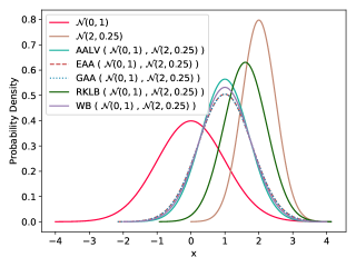
Figure 1: Comparison of statistical and geometric aggregations using univariate Gaussian distributions.

Fig. 1, presents a toy example of aggregation of two univariate Gaussian distributions, $p=\operatorname*{\mathcal{N}}(0,1)$ and $q=\operatorname*{\mathcal{N}}(2,0.25))$, with equal weights, $w_{p}=w_{q}=\tfrac{1}{2}$. This example illustrates the differences between the three statistical aggregation methods discussed above and the novel geometric aggregations RKLB and WB.

Metrics

To evaluate the performance of the considered FL algorithms in terms of accuracy, UQ, MC, and fairness, we employ the following metrics:

• Accuracy (Acc), which is employed to evaluate the performance of a classification model. In essence, accuracy provides a straightforward indication of how often the model makes correct predictions.

• Expected Calibration Error (ECE), which is a metric used to evaluate the calibration of probabilistic models, particularly in the context of classification tasks. Calibration refers to the alignment between predicted probabilities and actual outcomes. ECE provides a single scalar value summarizing the calibration of a model, the lower the ECE, the better calibrated the model is.

• Negative log likelihood (NLL), which is commonly used for optimizing neural networks in classification tasks. Additionally, NLL inherently involves probabilistic interpretations. A lower NLL indicates a better model fit, as it suggests that the model assigns higher probabilities to the true outcomes, implying a better uncertainty quantification.

• Average Accuracy ($\text{Acc}_{\text{avg}}$), which represents the average performance in a utilitarian view of fairness. It is formalized as:

  $$\text{Acc}_{\text{avg}}=\sum_{k=1}^{N}w_{k}\text{Acc}_{k}$$

  where $\text{Acc}_{k}$ is the accuracy of client $k$.

• Worst 10% Accuracies, which serves as a measure to evaluate the accuracy of the 10% worst performing clients, with an emphasis on egalitarian fairness.

Experimental Setup

In order to induce label shifts among the 10 clients participating in the FL scheme, we partition the samples of each label between the clients using a Dirichlet distribution as suggested in [50, 26, 51, 52, 53, 16]. Fig. 2 illustrates an example of such a split applied to the FashionMNIST dataset, where darker (resp. lighter) shades indicate higher (resp. lower) availability of data samples of the $i^{th}$ class at client $k$.

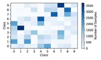
Figure 2: Example of a data split simulating the label shift.

We assign the aggregation weights to reflect the importance of each client in proportion to the volume of data locally owned, i.e., $w_{k}=\tfrac{|\mathcal{D}_{k}|}{|\mathcal{D}|}$ where $|\cdot|$ indicates the number of samples in the dataset.

The architecture of the global and local models consists of two convolutional layers and three fully connected layers. Following an HBDL approach, we implement the last $n=0,1,2,3$ layers as Bayesian fully connected layers, whereas the remaining layers are deterministic. In our comparative study, increasing $n$ allows measuring the impact of additional Bayesian layers on the UQ, MC, fairness, and the cost-effectiveness of the FL algorithm in time.

		FashionMNIST			CIFAR-10			SVHN
Nbl	Alg.	Acc $\uparrow$	ECE $\downarrow$	NLL $\downarrow$	Acc $\uparrow$	ECE $\downarrow$	NLL $\downarrow$	Acc $\uparrow$	ECE $\downarrow$	NLL $\downarrow$
0	FedAVG	87.88 $\operatorname*{{\scriptstyle\pm}}$ 0.79	9.42 $\operatorname*{{\scriptstyle\pm}}$ 0.62	0.76 $\operatorname*{{\scriptstyle\pm}}$ 0.04	61.63 $\operatorname*{{\scriptstyle\pm}}$ 3.11	12.17 $\operatorname*{{\scriptstyle\pm}}$ 2.21	1.18 $\operatorname*{{\scriptstyle\pm}}$ 0.11	86.06 $\operatorname*{{\scriptstyle\pm}}$ 0.45	10.56 $\operatorname*{{\scriptstyle\pm}}$ 0.46	1.01 $\operatorname*{{\scriptstyle\pm}}$ 0.06
1	AALV	88.22 $\operatorname*{{\scriptstyle\pm}}$ 0.34	8.59 $\operatorname*{{\scriptstyle\pm}}$ 0.27	0.67 $\operatorname*{{\scriptstyle\pm}}$ 0.02	63.42 $\operatorname*{{\scriptstyle\pm}}$ 3.02	8.63 $\operatorname*{{\scriptstyle\pm}}$ 1.37	1.09 $\operatorname*{{\scriptstyle\pm}}$ 0.09	86.52 $\operatorname*{{\scriptstyle\pm}}$ 0.29	8.67 $\operatorname*{{\scriptstyle\pm}}$ 0.45	0.81 $\operatorname*{{\scriptstyle\pm}}$ 0.05
	EAA	88.07 $\operatorname*{{\scriptstyle\pm}}$ 0.22	8.61 $\operatorname*{{\scriptstyle\pm}}$ 0.06	0.66 $\operatorname*{{\scriptstyle\pm}}$ 0.02	63.69 $\operatorname*{{\scriptstyle\pm}}$ 2.47	7.99 $\operatorname*{{\scriptstyle\pm}}$ 1.10	1.07 $\operatorname*{{\scriptstyle\pm}}$ 0.09	86.24 $\operatorname*{{\scriptstyle\pm}}$ 0.20	9.00 $\operatorname*{{\scriptstyle\pm}}$ 0.45	0.84 $\operatorname*{{\scriptstyle\pm}}$ 0.06
	GAA	88.15 $\operatorname*{{\scriptstyle\pm}}$ 0.31	8.49 $\operatorname*{{\scriptstyle\pm}}$ 0.25	0.66 $\operatorname*{{\scriptstyle\pm}}$ 0.01	63.66 $\operatorname*{{\scriptstyle\pm}}$ 2.22	8.49 $\operatorname*{{\scriptstyle\pm}}$ 2.06	1.08 $\operatorname*{{\scriptstyle\pm}}$ 0.09	86.36 $\operatorname*{{\scriptstyle\pm}}$ 0.28	8.73 $\operatorname*{{\scriptstyle\pm}}$ 0.44	0.82 $\operatorname*{{\scriptstyle\pm}}$ 0.06
	RKLB	88.07 $\operatorname*{{\scriptstyle\pm}}$ 0.36	8.61 $\operatorname*{{\scriptstyle\pm}}$ 0.20	0.67 $\operatorname*{{\scriptstyle\pm}}$ 0.01	63.37 $\operatorname*{{\scriptstyle\pm}}$ 2.62	8.21 $\operatorname*{{\scriptstyle\pm}}$ 1.31	1.08 $\operatorname*{{\scriptstyle\pm}}$ 0.09	86.26 $\operatorname*{{\scriptstyle\pm}}$ 0.26	8.80 $\operatorname*{{\scriptstyle\pm}}$ 0.32	0.82 $\operatorname*{{\scriptstyle\pm}}$ 0.04
	WB	88.34 $\operatorname*{{\scriptstyle\pm}}$ 0.30	8.39 $\operatorname*{{\scriptstyle\pm}}$ 0.29	0.67 $\operatorname*{{\scriptstyle\pm}}$ 0.02	63.91 $\operatorname*{{\scriptstyle\pm}}$ 2.64	8.62 $\operatorname*{{\scriptstyle\pm}}$ 1.63	1.08 $\operatorname*{{\scriptstyle\pm}}$ 0.09	86.55 $\operatorname*{{\scriptstyle\pm}}$ 0.37	8.66 $\operatorname*{{\scriptstyle\pm}}$ 0.56	0.82 $\operatorname*{{\scriptstyle\pm}}$ 0.06
2	AALV	87.62 $\operatorname*{{\scriptstyle\pm}}$ 0.45	7.93 $\operatorname*{{\scriptstyle\pm}}$ 0.23	0.60 $\operatorname*{{\scriptstyle\pm}}$ 0.01	65.03 $\operatorname*{{\scriptstyle\pm}}$ 2.92	7.07 $\operatorname*{{\scriptstyle\pm}}$ 1.62	1.03 $\operatorname*{{\scriptstyle\pm}}$ 0.09	85.46 $\operatorname*{{\scriptstyle\pm}}$ 0.10	7.66 $\operatorname*{{\scriptstyle\pm}}$ 0.53	0.77 $\operatorname*{{\scriptstyle\pm}}$ 0.04
	EAA	87.53 $\operatorname*{{\scriptstyle\pm}}$ 0.57	8.03 $\operatorname*{{\scriptstyle\pm}}$ 0.36	0.61 $\operatorname*{{\scriptstyle\pm}}$ 0.03	64.02 $\operatorname*{{\scriptstyle\pm}}$ 1.99	7.26 $\operatorname*{{\scriptstyle\pm}}$ 1.82	1.05 $\operatorname*{{\scriptstyle\pm}}$ 0.07	85.64 $\operatorname*{{\scriptstyle\pm}}$ 0.33	7.58 $\operatorname*{{\scriptstyle\pm}}$ 0.55	0.77 $\operatorname*{{\scriptstyle\pm}}$ 0.05
	GAA	87.82 $\operatorname*{{\scriptstyle\pm}}$ 0.64	7.68 $\operatorname*{{\scriptstyle\pm}}$ 0.44	0.60 $\operatorname*{{\scriptstyle\pm}}$ 0.03	64.59 $\operatorname*{{\scriptstyle\pm}}$ 3.51	7.65 $\operatorname*{{\scriptstyle\pm}}$ 2.40	1.04 $\operatorname*{{\scriptstyle\pm}}$ 0.12	85.54 $\operatorname*{{\scriptstyle\pm}}$ 0.44	7.63 $\operatorname*{{\scriptstyle\pm}}$ 0.70	0.77 $\operatorname*{{\scriptstyle\pm}}$ 0.04
	RKLB	87.59 $\operatorname*{{\scriptstyle\pm}}$ 0.57	8.01 $\operatorname*{{\scriptstyle\pm}}$ 0.38	0.63 $\operatorname*{{\scriptstyle\pm}}$ 0.03	65.20 $\operatorname*{{\scriptstyle\pm}}$ 3.99	6.87 $\operatorname*{{\scriptstyle\pm}}$ 2.33	1.01 $\operatorname*{{\scriptstyle\pm}}$ 0.11	85.57 $\operatorname*{{\scriptstyle\pm}}$ 0.45	7.64 $\operatorname*{{\scriptstyle\pm}}$ 0.79	0.77 $\operatorname*{{\scriptstyle\pm}}$ 0.05
	WB	87.69 $\operatorname*{{\scriptstyle\pm}}$ 0.74	7.96 $\operatorname*{{\scriptstyle\pm}}$ 0.60	0.62 $\operatorname*{{\scriptstyle\pm}}$ 0.03	64.74 $\operatorname*{{\scriptstyle\pm}}$ 3.29	7.39 $\operatorname*{{\scriptstyle\pm}}$ 2.22	1.03 $\operatorname*{{\scriptstyle\pm}}$ 0.10	85.57 $\operatorname*{{\scriptstyle\pm}}$ 0.51	7.65 $\operatorname*{{\scriptstyle\pm}}$ 0.60	0.76 $\operatorname*{{\scriptstyle\pm}}$ 0.05
3	AALV	88.07 $\operatorname*{{\scriptstyle\pm}}$ 0.58	5.55 $\operatorname*{{\scriptstyle\pm}}$ 0.56	0.45 $\operatorname*{{\scriptstyle\pm}}$ 0.03	63.71 $\operatorname*{{\scriptstyle\pm}}$ 3.63	4.89 $\operatorname*{{\scriptstyle\pm}}$ 1.34	1.01 $\operatorname*{{\scriptstyle\pm}}$ 0.09	86.15 $\operatorname*{{\scriptstyle\pm}}$ 0.80	2.62 $\operatorname*{{\scriptstyle\pm}}$ 0.62	0.53 $\operatorname*{{\scriptstyle\pm}}$ 0.04
	EAA	87.81 $\operatorname*{{\scriptstyle\pm}}$ 0.54	5.57 $\operatorname*{{\scriptstyle\pm}}$ 0.26	0.46 $\operatorname*{{\scriptstyle\pm}}$ 0.03	64.45 $\operatorname*{{\scriptstyle\pm}}$ 1.79	4.44 $\operatorname*{{\scriptstyle\pm}}$ 1.09	0.99 $\operatorname*{{\scriptstyle\pm}}$ 0.05	86.04 $\operatorname*{{\scriptstyle\pm}}$ 0.62	2.80 $\operatorname*{{\scriptstyle\pm}}$ 0.63	0.53 $\operatorname*{{\scriptstyle\pm}}$ 0.03
	GAA	88.02 $\operatorname*{{\scriptstyle\pm}}$ 0.55	5.42 $\operatorname*{{\scriptstyle\pm}}$ 0.28	0.45 $\operatorname*{{\scriptstyle\pm}}$ 0.03	64.40 $\operatorname*{{\scriptstyle\pm}}$ 2.30	4.13 $\operatorname*{{\scriptstyle\pm}}$ 0.71	0.99 $\operatorname*{{\scriptstyle\pm}}$ 0.06	86.27 $\operatorname*{{\scriptstyle\pm}}$ 1.02	2.69 $\operatorname*{{\scriptstyle\pm}}$ 0.72	0.53 $\operatorname*{{\scriptstyle\pm}}$ 0.05
	RKLB	87.77 $\operatorname*{{\scriptstyle\pm}}$ 0.80	5.75 $\operatorname*{{\scriptstyle\pm}}$ 0.40	0.46 $\operatorname*{{\scriptstyle\pm}}$ 0.03	64.55 $\operatorname*{{\scriptstyle\pm}}$ 2.97	4.55 $\operatorname*{{\scriptstyle\pm}}$ 0.83	1.00 $\operatorname*{{\scriptstyle\pm}}$ 0.08	86.53 $\operatorname*{{\scriptstyle\pm}}$ 1.03	2.76 $\operatorname*{{\scriptstyle\pm}}$ 0.84	0.52 $\operatorname*{{\scriptstyle\pm}}$ 0.05
	WB	87.54 $\operatorname*{{\scriptstyle\pm}}$ 0.54	5.77 $\operatorname*{{\scriptstyle\pm}}$ 0.23	0.46 $\operatorname*{{\scriptstyle\pm}}$ 0.03	64.30 $\operatorname*{{\scriptstyle\pm}}$ 2.55	4.12 $\operatorname*{{\scriptstyle\pm}}$ 1.18	1.00 $\operatorname*{{\scriptstyle\pm}}$ 0.07	85.99 $\operatorname*{{\scriptstyle\pm}}$ 0.68	2.91 $\operatorname*{{\scriptstyle\pm}}$ 0.58	0.54 $\operatorname*{{\scriptstyle\pm}}$ 0.03

Table 1: Accuracy, Model Calibration, and Uncertainty Quantification Results. The table compares the performance of the global models resulting of FedAVG, BFLAVG with different aggregation methods; AALV, EAA, GAA and BA-BFL with RKL barycenter (RKLB) and Wasserstein-2 barycenter (WB). The methods are grouped based on the number of Bayesian layers (Nbl) used in the models’ architecture. The evaluation is performed on three datasets (FashionMNIST, CIFAR-10, and SVHN) using the metrics of Accuracy (Acc), Expected Calibration Error (ECE), and Negative Log-Likelihood (NLL).

Overview of the Results

Table 1 shows that the compared aggregation methods using the same models’ architecture, i.e., the same number of Bayesian layers, yield similar scores, suggesting comparable performance across the evaluated metrics. Depending on the score and dataset, it is difficult to conclusively determine the best method.

The datasets used (FashionMNIST, SVHN, CIFAR-10) present different levels of difficulty. State-of-the-art results in heterogeneous settings indicate that the CIFAR-10 task is the most challenging, as evidenced by lower accuracy, higher ECE and NLL, and longer training times, compared to the tasks involving FashionMNIST and SVHN.

Comparing all the Bayesian algorithms discussed in this paper with FedAVG as the deterministic baseline, we observe that incorporating Bayesian methods significantly enhances UQ and MC, as evidenced by improvements in ECE and NLL. This performance is achieved while maintaining similar global accuracy on FashionMNIST and SVHN and outperforming FedAVG on CIFAR-10. This superior performance on CIFAR-10 can be attributed to the task’s increased difficulty in the heterogeneous setting, where Bayesian methods provide a noticeable advantage.

By examining the results in Table 1 and Figs. 3, 4, and 5, we observe some trends depending on the number of Bayesian layers present, allowing us to analyze various aspects, including UQ, MC, fairness, and cost-effectiveness:

• UQ and MC: Regardless of the Bayesian algorithm used, the trends reported in Fig. 3 indicate that incorporating a greater number of Bayesian layers into the local models improves both global MC and UQ while reducing the ECE and NLL scores.

  

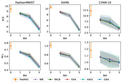
  Figure 3: Effect of Bayesian Layers on UQ and MC.

• Cost-effectiveness: Increasing the number of Bayesian layers offers the significant advantage of enhancing UQ and MC. However, this increased Bayesian complexity often comes at the cost of reduced time efficiency. As the number of Bayesian layers increases, the computational demand grows, leading to longer processing time per communication round, as demonstrated in Fig. 4. This trade-off between improved model reliability and increased complexity must be carefully considered in practical applications.

  

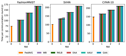
  Figure 4: Effect of Bayesian Layers on Cost-Effectiveness.

• Fairness: The observed trend in Fig. 5 indicates that incorporating more Bayesian layers tends to decrease the fairness of the algorithm between the different clients on the Fashion-MNIST and SVHN datasets, suggesting a trade-off between UQ and fairness. Conversely, on the CIFAR-10 dataset, which presents a more complex task as explained above, we observe an improvement in fairness with an increasing number of Bayesian layers. This may suggest that the relationship between Bayesian complexity and fairness is influenced by the nature of the dataset and task complexity. Notably, based on the results from our exploration of CIFAR-10 under the heterogeneous setting, we can assert that adopting a Bayesian approach for challenging tasks can enhance not only fairness, but also accuracy, UQ, and MC.

  

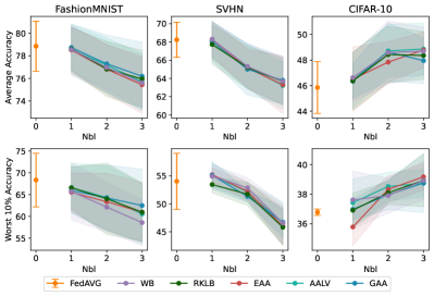
  Figure 5: Effect of Bayesian Layers on Fairness.

5 Conclusions

In this paper, we proposed BA-BFL, a novel geometric interpretation of barycenters as a solution to the BFL aggregation problem. Following this idea, we proposed two aggregation techniques based on the analytical results of Gaussian barycenters derived for two widely-used divergences, squared Wasserstein-2 distance and reverse KL divergence. We experimentally tested the proposed methods in a heterogeneous setting, showing performances similar to existing statistical aggregation methods. In the same setting, we also examined the impact of varying the number of Bayesian layers in an HBDL context on accuracy, uncertainty quantification, model calibration, cost-effectiveness, and fairness.

For future work, we envision several extensions to our study, including expanding the family of distributions to incorporate non-parametric distributions and investigating alternative divergences. Additionally, we aim to address the personalization problem within the context of barycentric aggregation in BFL.

References

- [1] Brendan McMahan, Eider Moore, Daniel Ramage, Seth Hampson, and Blaise Aguera y Arcas. Communication-efficient learning of deep networks from decentralized data. In Artificial intelligence and statistics, pages 1273–1282. PMLR, 2017.
- [2] Pian Qi, Diletta Chiaro, Antonella Guzzo, Michele Ianni, Giancarlo Fortino, and Francesco Piccialli. Model aggregation techniques in federated learning: A comprehensive survey. Future Generation Computer Systems, 2023.
- [3] Qinbin Li, Yiqun Diao, Quan Chen, and Bingsheng He. Federated learning on non-iid data silos: An experimental study. In 2022 IEEE 38th international conference on data engineering (ICDE), pages 965–978. IEEE, 2022.
- [4] Peter Kairouz, H Brendan McMahan, Brendan Avent, Aurélien Bellet, Mehdi Bennis, Arjun Nitin Bhagoji, Kallista Bonawitz, Zachary Charles, Graham Cormode, Rachel Cummings, et al. Advances and open problems in federated learning. Foundations and trends® in machine learning, 14(1–2):1–210, 2021.
- [5] Yuyang Deng, Mohammad Mahdi Kamani, and Mehrdad Mahdavi. Adaptive personalized federated learning. arXiv preprint arXiv:2003.13461, 2020.
- [6] Canh T Dinh, Nguyen Tran, and Josh Nguyen. Personalized federated learning with moreau envelopes. Advances in neural information processing systems, 33:21394–21405, 2020.
- [7] Alireza Fallah, Aryan Mokhtari, and Asuman Ozdaglar. Personalized federated learning: A meta-learning approach. arXiv preprint arXiv:2002.07948, 2020.
- [8] Ninareh Mehrabi, Fred Morstatter, Nripsuta Saxena, Kristina Lerman, and Aram Galstyan. A survey on bias and fairness in machine learning. ACM computing surveys (CSUR), 54(6):1–35, 2021.
- [9] Nripsuta Ani Saxena, Karen Huang, Evan DeFilippis, Goran Radanovic, David C Parkes, and Yang Liu. How do fairness definitions fare? examining public attitudes towards algorithmic definitions of fairness. In Proceedings of the 2019 AAAI/ACM Conference on AI, Ethics, and Society, pages 99–106, 2019.
- [10] Yuxin Shi, Han Yu, and Cyril Leung. Towards fairness-aware federated learning. IEEE Transactions on Neural Networks and Learning Systems, 2023.
- [11] Yuwei Zhang, Tong Xia, Abhirup Ghosh, and Cecilia Mascolo. Uncertainty quantification in federated learning for heterogeneous health data. In International Workshop on Federated Learning for Distributed Data Mining, 2023.
- [12] Nikolas Koutsoubis, Yasin Yilmaz, Ravi P Ramachandran, Matthew Schabath, and Ghulam Rasool. Privacy preserving federated learning in medical imaging with uncertainty estimation. arXiv preprint arXiv:2406.12815, 2024.
- [13] Shrey Bhatt, Aishwarya Gupta, and Piyush Rai. Federated learning with uncertainty via distilled predictive distributions. In Asian Conference on Machine Learning, pages 153–168. PMLR, 2024.
- [14] Xu Zhang, Yinchuan Li, Wenpeng Li, Kaiyang Guo, and Yunfeng Shao. Personalized federated learning via variational bayesian inference. In International Conference on Machine Learning, pages 26293–26310. PMLR, 2022.
- [15] Nikita Kotelevskii, Maxime Vono, Alain Durmus, and Eric Moulines. Fedpop: A bayesian approach for personalised federated learning. Advances in Neural Information Processing Systems, 35:8687–8701, 2022.
- [16] Atahan Ozer, Kadir Burak Buldu, Abdullah Akgül, and Gozde Unal. How to combine variational bayesian networks in federated learning. arXiv preprint arXiv:2206.10897, 2022.
- [17] John Fischer, Marko Orescanin, Justin Loomis, and Patrick McClure. Federated bayesian deep learning: The application of statistical aggregation methods to bayesian models. arXiv preprint arXiv:2403.15263, 2024.
- [18] Jiaming Zeng, Adam Lesnikowski, and Jose M Alvarez. The relevance of bayesian layer positioning to model uncertainty in deep bayesian active learning. arXiv preprint arXiv:1811.12535, 2018.
- [19] Eric Maskin. A theorem on utilitarianism. The Review of Economic Studies, 45(1):93–96, 1978.
- [20] John Rawls. Some reasons for the maximin criterion. The American Economic Review, 64(2):141–146, 1974.
- [21] John Rawls. A theory of justice. revised edition, 1999.
- [22] Guojun Zhang, Saber Malekmohammadi, Xi Chen, and Yaoliang Yu. Proportional fairness in federated learning. arXiv preprint arXiv:2202.01666, 2022.
- [23] Theodore Papamarkou, Maria Skoularidou, Konstantina Palla, Laurence Aitchison, Julyan Arbel, David Dunson, Maurizio Filippone, Vincent Fortuin, Philipp Hennig, Aliaksandr Hubin, et al. Position paper: Bayesian deep learning in the age of large-scale ai. arXiv preprint arXiv:2402.00809, 2024.
- [24] Laurent Valentin Jospin, Hamid Laga, Farid Boussaid, Wray Buntine, and Mohammed Bennamoun. Hands-on bayesian neural networks—a tutorial for deep learning users. IEEE Computational Intelligence Magazine, 17(2):29–48, 2022.
- [25] Longbing Cao, Hui Chen, Xuhui Fan, Joao Gama, Yew-Soon Ong, and Vipin Kumar. Bayesian federated learning: A survey. arXiv preprint arXiv:2304.13267, 2023.
- [26] Mikhail Yurochkin, Mayank Agarwal, Soumya Ghosh, Kristjan Greenewald, Nghia Hoang, and Yasaman Khazaeni. Bayesian nonparametric federated learning of neural networks. In International conference on machine learning, pages 7252–7261. PMLR, 2019.
- [27] Mahrokh Ghoddousi Boroujeni, Andreas Krause, and Giancarlo Ferrari Trecate. Personalized federated learning of probabilistic models: A pac-bayesian approach. arXiv preprint arXiv:2401.08351, 2024.
- [28] Junyi Zhu, Xingchen Ma, and Matthew B Blaschko. Confidence-aware personalized federated learning via variational expectation maximization. In Proceedings of the IEEE/CVF Conference on Computer Vision and Pattern Recognition, pages 24542–24551, 2023.
- [29] Liangxi Liu, Xi Jiang, Feng Zheng, Hong Chen, Guo-Jun Qi, Heng Huang, and Ling Shao. A bayesian federated learning framework with online laplace approximation. IEEE Transactions on Pattern Analysis and Machine Intelligence, 2023.
- [30] Mohsin Hasan, Guojun Zhang, Kaiyang Guo, Xi Chen, and Pascal Poupart. Calibrated one round federated learning with bayesian inference in the predictive space. In Proceedings of the AAAI conference on artificial intelligence, volume 38, pages 12313–12321, 2024.
- [31] Han Guo, Philip Greengard, Hongyi Wang, Andrew Gelman, Yoon Kim, and Eric P Xing. Federated learning as variational inference: A scalable expectation propagation approach. arXiv preprint arXiv:2302.04228, 2023.
- [32] Hong-You Chen and Wei-Lun Chao. Fedbe: Making bayesian model ensemble applicable to federated learning. arXiv preprint arXiv:2009.01974, 2020.
- [33] Maruan Al-Shedivat, Jennifer Gillenwater, Eric Xing, and Afshin Rostamizadeh. Federated learning via posterior averaging: A new perspective and practical algorithms. arXiv preprint arXiv:2010.05273, 2020.
- [34] Luca Corinzia, Ami Beuret, and Joachim M Buhmann. Variational federated multi-task learning. arXiv preprint arXiv:1906.06268, 2019.
- [35] N. Cressie and T. Read. Goodness-of-Fit Statistics for Discrete Multivariate Data. Springer: New York, NY, USA, 1988.
- [36] Matthias Gelbrich. On a formula for the l2 Wasserstein metric between measures on Euclidean and Hilbert spaces. Mathematische Nachrichten, 147(1):185–203, 1990.
- [37] Shun-ichi Amari. Information Geometry and its Applications, volume 194. Springer, 2016.
- [38] I. Csiszár. -Divergence Geometry of Probability Distributions and Minimization Problems. The Annals of Probability, 3(1):146 – 158, 1975.
- [39] I. Csiszar and F. Matus. Information projections revisited. IEEE Transactions on Information Theory, 49(6):1474–1490, 2003.
- [40] Frank Nielsen and Richard Nock. Sided and symmetrized bregman centroids. IEEE Transactions on Information Theory, 55(6):2882–2904, 2009.
- [41] Alessandro D’Ortenzio, Costanzo Manes, and Umut Orguner. Fixed-point iterative computation of gaussian barycenters for some dissimilarity measures. In 2022 International Conference on Computational Science and Computational Intelligence (CSCI), pages 1422–1428, 2022.
- [42] Michael I Jordan, Zoubin Ghahramani, Tommi S Jaakkola, and Lawrence K Saul. An introduction to variational methods for graphical models. Machine learning, 37:183–233, 1999.
- [43] David M Blei, Alp Kucukelbir, and Jon D McAuliffe. Variational inference: A review for statisticians. Journal of the American statistical Association, 112(518):859–877, 2017.
- [44] Giorgio Battistelli and Luigi Chisci. Kullback–leibler average, consensus on probability densities, and distributed state estimation with guaranteed stability. Automatica, 50(3):707–718, 2014.
- [45] Martial Agueh and Guillaume Carlier. Barycenters in the wasserstein space. SIAM Journal on Mathematical Analysis, 43(2):904–924, 2011.
- [46] Giuseppe Serra, Photios A. Stavrou, and Marios Kountouris. On the computation of the gaussian rate–distortion–perception function. IEEE Journal on Selected Areas in Information Theory, 5:314–330, 2024.
- [47] Han Xiao, Kashif Rasul, and Roland Vollgraf. Fashion-mnist: a novel image dataset for benchmarking machine learning algorithms. arXiv preprint arXiv:1708.07747, 2017.
- [48] Alex Krizhevsky. Learning multiple layers of features from tiny images. Technical report, 2009.
- [49] Yuval Netzer, Tao Wang, Adam Coates, Alessandro Bissacco, Baolin Wu, Andrew Y Ng, et al. Reading digits in natural images with unsupervised feature learning. In NIPS workshop on deep learning and unsupervised feature learning, volume 2011, page 4. Granada, 2011.
- [50] Qinbin Li, Bingsheng He, and Dawn Song. Practical one-shot federated learning for cross-silo setting. arXiv preprint arXiv:2010.01017, 2020.
- [51] Hongyi Wang, Mikhail Yurochkin, Yuekai Sun, Dimitris Papailiopoulos, and Yasaman Khazaeni. Federated learning with matched averaging. arXiv preprint arXiv:2002.06440, 2020.
- [52] Jianyu Wang, Qinghua Liu, Hao Liang, Gauri Joshi, and H Vincent Poor. Tackling the objective inconsistency problem in heterogeneous federated optimization. Advances in neural information processing systems, 33:7611–7623, 2020.
- [53] Tao Lin, Lingjing Kong, Sebastian U Stich, and Martin Jaggi. Ensemble distillation for robust model fusion in federated learning. Advances in Neural Information Processing Systems, 33:2351–2363, 2020.