A Mapper algorithm with implicit intervals and its optimization

Abstract

The Mapper algorithm is an essential tool for visualizing complex, high dimensional data in topology data analysis (TDA) and has been widely used in biomedical research. It outputs a combinatorial graph whose structure implies the shape of the data. However,the need for manual parameter tuning and fixed intervals, along with fixed overlapping ratios may impede the performance of the standard Mapper algorithm. Variants of the standard Mapper algorithms have been developed to address these limitations, yet most of them still require manual tuning of parameters. Additionally, many of these variants, including the standard version found in the literature, were built within a deterministic framework and overlooked the uncertainty inherent in the data. To relax these limitations, in this work, we introduce a novel framework that implicitly represents intervals through a hidden assignment matrix, enabling automatic parameter optimization via stochastic gradient descent. In this work, we develop a soft Mapper framework based on a Gaussian mixture model(GMM) for flexible and implicit interval construction. We further illustrate the robustness of the soft Mapper algorithm by introducing the Mapper graph mode as a point estimation for the output graph. Moreover, a stochastic gradient descent algorithm with a specific topological loss function is proposed for optimizing parameters in the model. Both simulation and application studies demonstrate its effectiveness in capturing the underlying topological structures. In addition, the application to an RNA expression dataset obtained from the Mount Sinai/JJ Peters VA Medical Center Brain Bank (MSBB) successfully identifies a distinct subgroup of Alzheimer’s Disease. The implementation of our method is available at https://github.com/FarmerTao/Implicit-interval-Mapper.git.

1 Introduction

The Mapper algorithm is a powerful tool in topology data analysis (TDA) used to explore the shape of datasets. Initially introduced for 3D object recognition (Singh et al., 2007), the Mapper algorithm has demonstrated remarkable efficiency in extracting topological information across various data types. Its application spans various areas, notably in biomedical research (Skaf and Laubenbacher, 2022). For example, it successfully identified new breast cancer subgroups with superior survival rates (Nicolau et al., 2011). In single cell RNA-Seq analysis, a Mapper-based algorithm was used to study unbiased temporal transcriptional regulation (Rizvi et al., 2017). The variants of Mapper algorithms were also used to uncover higher-order structures of complex phenomics data (Kamruzzaman et al., 2021). Moreover, many efforts have been made to integrate the Mapper algorithm with other machine learning techniques. For instance, Bodnar et al. (2021) enhanced the performance of a graph neural network by incorporating the Mapper algorithm as a pooling operation. When combined with autoencoders, the Mapper algorithm can be used as a robust classifier (Cyranka et al., 2019), remedying the shortcomings of traditional convolutional neural networks, such as susceptibility to gradient-based attacks. Recently, a visualization method called ShapeVis which was inspired by the Mapper algorithm was proposed to produce more concise topological structure than standard Mapper graph (Kumari et al., 2020). Besides advances of the Mapper algorithms in applications, there has been some new progress in theory. Carrière et al. (2018) analyzed the Mapper algorithm from statistical perspective and introduced a novel method for parameter selection. Other studies have explored the algorithm’s convergence to Reeb graphs (Brown et al., 2021), and examined its topological properties (Dey et al., 2017).

The standard Mapper algorithm generates a graph that captures the shape of the data by dividing the support of the filtered data into several overlapped intervals with a fixed length (Singh et al., 2007). The major limitations of the standard Mapper algorithm are the requirements of fixed length of intervals and overlapping rate. Many algorithms were proposed to address these limitations. For instance, F-Mapper (Bui et al., 2020) utilized the fuzzy clustering algorithm to allow flexible interval partitioning by introducing an additional threshold parameter to control the degree of overlap. However, the introduction of the parameter also increased the algorithm’s computational complexity. In a different vein, the ensemble version of Mapper was proposed by Kang and Lim (2021); Fitzpatrick et al. (2023), which can recover the topology of datasets without parameter tuning. However, this method has a significant high computational cost due to the execution of multiple instances of the Mapper algorithm. Differently, the Ball Mapper (Dłotko, 2019) directly constructed cover on a given dataset, avoiding the difficulty of choosing filter functions. Nevertheless, its construction process is somewhat arbitrary and could inadvertently introduce extra parameters, increasing computational complexity. The D-Mapper, as introduced by Tao and Ge (2024), developed a probabilistic framework to construct intervals of the projected data based on a mixture distribution. This approach offers flexibility in interval construction. Additionally, the Soft Mapper, proposed by Oulhaj et al. (2024), a smoother version of the standard Mapper algorithm. This algorithm focused on the optimization of filter functions by minimizing the topological loss.

In this study, our objective is to enhance the Mapper algorithm by incorporating a probability model that requires fewer parameter selections and enables flexible interval partitioning. Inspired by the D-Mapper (Tao and Ge, 2024), our approach utilizes a mixture distribution. Still, it implicitly represents intervals through a hidden assignment matrix, eliminating the need for the interval threshold $\alpha$. This framework optimizes the mixture distribution by integrating stochastic gradient descent, facilitating automatic parameter tuning. This research contributes three key innovations as follows. First, we introduce a novel framework for constructing Mapper graphs based on mixture models, enabling flexible and implicit interval definitions. Second, we consider the uncertainty in a Mapper graph and introduce a mode-based estimation for the Mapper graph. Finally, we develop a stochastic gradient descent algorithm to optimize these intervals, resulting in an improved Mapper graph.

In addition, the simulation results show that our method is comparable to the standard Mapper algorithm and is more robust. Our model is also applied to an RNA expression dataset obtained from the Mount Sinai/JJ Peters VA Medical Center Brain Bank (MSBB) (Wang et al., 2018) and successfully identifies a distinct subgroup of Alzheimer’s Disease.

2 Preliminary

2.1 Mapper algorithm

The Mapper algorithm has been widely used to output a graph of a given dataset to represent its topological structure (Dey et al., 2017), the output graph can be regarded as a discrete version of the Reeb graph. The core concept of the Mapper algorithm is as follows. First, it projects a given high-dimensional dataset into a lower-dimensional space. Then, it constructs a reasonable cover for the projected data and pulls back the original data points according to each interval and clustering. Finally, each cluster is treated as a node of the output graph, and an edge is added between two clusters if they share any data points.

Consider a dataset with $n$ data points, $\{\boldsymbol{x_{1}},\ldots,\boldsymbol{x_{n}}\}$, $\boldsymbol{x_{i}}\in\mathbb{R}^{d}$, $i=1,\ldots,n$. Let $\mathbb{X}_{n}$ be the support of this dataset. Denote $f(\cdot):\mathbb{X}^{n}\rightarrow\mathbb{R}^{m}$, $m<n$, a single-valued filter function, which maps each data point from $\mathbb{X}^{n}$ to a lower-dimensional space, $\mathbb{R}^{m}$ ($m\geq 1$). As in most of literature Bui et al. (2020); Kang and Lim (2021); Fitzpatrick et al. (2023), here $m$ is set to $1$. We use a simple example to illustrate the Mapper algorithm. The example dataset has a cross shape, as shown in Figure 1 (a). The Mapper algorithm first projects data onto a real line using a filter function, $f(\boldsymbol{x})=y,~\boldsymbol{x}\in\mathbb{R}^{2},~y\in\mathbb{R}$, as shown in the upper pannel of Figure 1 (b), the filter function is set to $f(\boldsymbol{x})=\frac{1}{n}\sum_{i=1}^{n}||\boldsymbol{x}-\boldsymbol{x}_{i}||$, i.e. the mean distance of $\boldsymbol{x}$ to all points $\boldsymbol{x}_{i}$, $i=1,\ldots,n$. Set $a=\min\{f(\boldsymbol{x}_{i}),i=1,\ldots,n\}$, $b=\max\{f(\boldsymbol{x}_{i}),i=1,\ldots,n\}$. Then divide $[a,b]$ into $K$ equal length intervals with $p$ percentage overlapping ratio between any two adjacent intervals, denoted as $I_{j}=[a_{j},b_{j}]$, $j=1,\ldots,K$, as shown in the lower panel of Figure 1 (b). These intervals such that $[a,b]=\bigcup_{j=1}^{K}I_{j}$, $|b_{j}-a_{j+1}|=p|b_{1}-a_{1}|$, $j=1,\ldots,n-1$, where $a=a_{1}<b_{1}<a_{2}<\ldots<a_{n}<b_{n-1}<b_{n}=b$.

Each interval $I_{j}$ is then pulled back to the original space through the inverse mapping $f^{-1}(I_{j}),j=1,...,K$. A clustering algorithm is applied to original data points fall into each $f^{-1}(I_{j})$, partitioning the points into $r_{j}$ disjoint clusters, represented as $C_{j,i}$, $i=1,\ldots,r_{j}$, such that $\bigcup_{r_{j}}C_{j,r_{j}}\subset f^{-1}(I_{j})$ ,where $j=1,...,K$. By pulling back all intervals, we can define a pull back cover $C=\{C_{1,1},...,C_{1,r_{1}},...,C_{K,1},...,C_{K,r_{K}}\}$. The Mapper graph is constructed from this cover, where each cluster in $C$ corresponds to a node in the graph. An edge is added between any two nodes if their corresponding clusters intersect, i.e., if $C_{i,j}\cap C_{i^{\prime},j^{\prime}}\neq\varnothing$. As shown in Figure 1 (c), the resulting Mapper graph accurately captures the shape of the data.

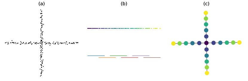
Figure 1: A demonstration of the Mapper algorithm applied to a dataset with a cross structure. (a) A visualization of the dataset. (b) The projected data and its overlapped intervals when $K=6$, $p=0.33$. (c) The output graph of the Mapper algorithm. The clustering algorithm implemented here is the DBSCAN$(\epsilon=0.6,minPts=5)$ (Schubert et al., 2017). The output Mapper graph presents a cross shape, which is consistent with the shape of the dataset.

2.2 Soft Mapper

Traditional Mapper graphs are constructed through intervals based on the filtered data. The soft Mapper constructs Mapper graphs with a hidden assignment matrix without requiring fixed intervals (Oulhaj et al., 2024). The hidden assignment matrix is a ${n\times K}$ matrix, depicts the allocation relationship between given $n$ data points and $K$ groups. This matrix is denoted as $H=(H_{ij})_{n\times K}$, in which $H_{ij}=1$ if the $i$-th point belongs to $j$-th interval, otherwise $H_{ij}=0$, for $i=1,\ldots,n,~j=1,\ldots,K$. With a hidden assignment matrix $H$, a Mapper graph is constructed directly through the standard process of pulling back and clustering, which we refer to as a Mapper function, defined as follows.

Definition 1 (Mapper function).

A Mapper function $\phi:H\mapsto G$, is a map from a hidden assignment matrix $H$ to a Mapper graph $G$. This function includes pulling back and clustering operations.

When a hidden assignment matrix $H$ is a random matrix, the soft Mapper can be viewed as a stochastic version of the Mapper, parametrized by a Mapper function $\phi$ and a probability density function defined over a hidden assignment matrix $H$. The resulting random graph $G=\phi(H)$ is a function of a hidden assignment matrix $H$. The simplest example of a soft Mapper is obtained by assigning a Bernoulli distribution to each element $H_{ij}$ of a hidden assignment matrix $H$.

Definition 2 (Soft Mapper with a Bernoulli distribution).

Suppose $H_{ij}$ follows a Bernoulli distribution with parameter $Q_{ij}$,

$$H_{ij}\sim\mathcal{B}(Q_{ij}),~i=1,\ldots,n,j=1,\ldots,K.$$

Where $Q=(Q_{ij})_{n\times K}$ is a probability matrix of the Bernoulli distributions. Each element of a hidden assignment matrix $H$ can be drawn independently from a Bernoulli distribution with probability of success $Q_{ij}$, $0\leq O_{ij}\leq 1$ for $i=1,\ldots,n,~j=1,\ldots,K$.

With this definition, the model inference is simplified to estimate the probability matrix $Q$, which will yield the distribution of the Mapper graph. However, explicitly estimating $Q$ is challenging. In this work, we address this issue by making certain modifications to the soft Mapper approach.

3 Methods

3.1 GMM Soft Mapper

By incorporating a Gaussian Mixture Model, we can naturally define a hidden assignment matrix $H$ through soft clustering, and a probability matrix $Q$ can be easily derived from the GMM parameters. We fit a GMM to the projected data $\{y_{1},...,y_{n}\}$. As a result, the $Q_{ij}$ represents the probability that data point $y_{i}$ is assigned to $j$-th class within the GMM framework.

Definition 3 (GMM Soft Mapper).

Assuming that the projected data $\{y_{1},...,y_{n}\}$ follows a Gaussian mixture distribution. We define the weights, means, and variances of each component as $\boldsymbol{\pi}=\{\pi_{1},\dots,\pi_{K}\}$, $\boldsymbol{\mu}=\{\mu_{1},\dots,\mu_{K}\}$, $\boldsymbol{\sigma^{2}}=\{\sigma_{1}^{2},\dots,\sigma_{K}^{2}\}$, respectively. The set $\boldsymbol{\theta}=\{\boldsymbol{\pi},\boldsymbol{\mu},\boldsymbol{\sigma^{2}}\}$ denotes all model parameters. Conditional on $\boldsymbol{\theta}$, the distribution of each data point $y_{i}$ is given by:

$$y_{i}|\boldsymbol{\theta}\sim\sum_{k=1}^{K}\pi_{k}\mathcal{N}(y_{i}|\mu_{k},\sigma_{k}^{2}).$$

Then, for each point $y_{i}$, it is natural to set the probability of $y_{i}$ belonging to $j$-th class as follows,

$$Q_{ij}(y_{i})=\frac{\pi_{j}\mathcal{N}(y_{i}|\mu_{j},\sigma_{j}^{2})}{\sum_{k=1}^{K}\pi_{k}\mathcal{N}(y_{i}|\mu_{k},\sigma_{k}^{2})}.$$

where $i=1,\dots,n,j=1,\dots,K$. This GMM-based assignment scheme imposes an implicit constraint on each row of the probability matrix $Q$, such that the sum of the probabilities for each data point equals one, $\sum_{j=1}^{K}Q_{ij}=1$. However, the independent Bernoulli distribution assignment scheme of $H_{ij}$ in the Soft Mapper may lead to extreme assignments, some points being unassigned to any clusters or a point is being assigned to all clusters. For instance, if $K=4$, data point $y_{i}$ might have an assignment probability vector of $Q_{i.}=[0.3,0.2,0.4,0.1]$, $i=1,\ldots,n$. Then the independent Bernoulli distribution assignment scheme may result an assignment vector $H_{i.}=[0,0,0,0]$, which means the data point $y_{i}$ is being unassigned to any clusters, or $H_{i.}=[1,1,1,1]$, which means the data point $y_{i}$ belongs to all clusters. The former case violates the Mapper algorithm requirement that each data point belongs to at least one cluster, and the extreme case of being unassigned to any clusters should be avoided. The latter case conflicts with that fact the a data point in the Mapper algorithms typically falls into, at most, two adjacent intervals. Therefore, we propose a GMM-multinomial soft Mapper approach. Instead of sampling each element of $H$ independent through the Bernoulli distributions, we sample each row of the assignment matrix $H$ through a multinomial distributionconcerning each row of the probability matrix $Q$. The multinomial distribution grantees that each point is assigned to at least to one cluster, and at most to $m$ clusters as follows.

Definition 4 (Soft Mapper with a multinomial distribution).

Let $Q_{i\cdot}=(Q_{i1},\ldots,Q_{iK})$ represent the $i$-th row column of $Q$, and $H_{i\cdot}=(H_{i1},\ldots,H_{iK})$ represent the $i$-th row column of hidden assignment matrix $H$, $i=1,\dots,n,j=1,\dots,K$. Assume each row $H_{i\cdot}$ follows a multinomial distribution with total number of events $m=2$ and event probability vector $Q_{i.}$,

$$H_{.}\sim{Multi}(m,~Q_{i.}),~i=1,\ldots,n.$$

Here $H_{ij}$ may take values from $\{0,1,2\}$, and $H_{ij}\geq 1$ indicates that the $i$-th point is assigned to $j$-th interval, otherwise $H_{ij}=0$. For ease of notations, we denote $H\sim{Multi}(m,~Q)$ to indicate that each row of $H$ independently follows a multinomial distribution with event number parameter $m=2$ and event probabilities being each row of $Q$.

Our proposed soft Mapper samples each row $H_{i\cdot}$ independently from a multinomial distribution ${Multi}(2,Q_{i\cdot}),~i=1,\ldots,n.$. The total events $m$ of the multinomial distribution is set to $2$, guaranteeing that each data point can be assigned to at least one class and no more than two classes. This setting is reasonable, as in the Mapper algorithm, a data point typically falls within at least one interval and at most two adjacent intervals.

Our approach differs from the soft Mapper described in Oulhaj et al. (2024) in two key ways. Firstly, by using a GMM model, our $Q_{ij}$ can be specified as a function of the parameters $\boldsymbol{\theta}$. Thus, updating the GMM parameters $\boldsymbol{\theta}$ is equivalent to update $Q$. Whereas $Q$ in Oulhaj et al. (2024) was determined by the parameters in the filter functions. Secondly, we use an independent multinomial distribution assignment scheme to sample each row of the hidden assignment matrix $H$. The multinomial distribution avoids extreme cases where a data point is unassigned to any clusters or assigned to too many clusters.

3.2 The Mapper graph mode

The soft Mapper is a probabilistic version of the Mapper algorithm, where a random hidden assignment matrix $H$ can result in varying Mapper graphs. Although the topological structures of these soft Mapper graphs differ in detail, they often share some common features as they are derived from the same underlying distribution. We aim to obtain a Mapper graph that encapsulates all these common structures as its final representation. Since $H$ is a random discrete matrix, and each row is independently distributed, we can take the matrix of which each row is the mode of each row of $H$ as the mode representation of $H$ and then apply the Mapper function to get a Mapper graph, which we call the Mapper graph mode. The mode of a multinomial distribution has an explicit formula, allowing us to compute the mode of the Mapper graph directly and efficiently.

Definition 5 (The mode of a soft Mapper with a multinomial distribution).

For a soft Mapper with a multinomial distribution, each row follows an independent multinomial distribution. Given the $i$-th row of $Q$, we define,

$$Q_{i}^{*}=\max\{Q_{i1},...,Q_{iK}\},$$

$$i^{*}=\mathop{\arg\max}\limits_{i1,...,iK}\{Q_{i1},...,Q_{iK}\},$$

$$Q_{i}^{**}=\max\{Q_{i1},...,Q_{iK}\}\setminus\{Q_{i}^{*}\},$$

$${i}^{**}=\mathop{\arg\max}\limits_{\{i1,...,iK\}\setminus\{i^{*}\}}\{Q_{i1},...,Q_{iK}\}\setminus\{Q_{i}^{*}\}.$$

Here, the $Q_{i}^{*}$ and $Q_{i}^{**}$ are the largest and the second largest elements of $i$-th row of $Q$, respectively. ${i}^{*}$ and ${i}^{**}$ are their corresponding indices. For $i=1,\ldots,n,$, the mode of the $i$-th row of the hidden assignment matrix is then determined as follows (see Appendix A for the theoretical derivation).

If $\frac{1}{2}Q_{i}^{*}>Q_{i}^{**}$,

$$H_{mode}({i,j})=\begin{cases}1&\text{if }j=i^{*},\\ 0&\text{else}.\end{cases}$$

If $\frac{1}{2}Q_{i}^{*}\leq Q_{i}^{**}$,

$$H_{mode}({i,j})=\begin{cases}1&\text{if }j=i^{*},i^{**},\\ 0&\text{else}.\end{cases}$$

The mode of Mapper graph can be defined by a Mapper function and the mode of hidden assignment matrix $H_{mode}$,

$$G_{mode}=\phi(H_{mode}).$$

The explicit form of the $H_{mode}$ significantly reduces the computational burden of the algorithm. In the following sections, we will adopt the mode of the Mapper graph as the representation of the graph and present several Mapper graph samples to illustrate the inherent uncertainty of these graphs.

3.3 Loss function

The probability matrix $Q$ is derived from a Gaussian mixture model fitted to the projected data. Therefore, optimizing the Mapper graph is equivalent to optimizing the parameter $\boldsymbol{\theta}$ of GMM. However, the maximum likelihood estimation of parameter $\boldsymbol{\theta}$ only accounts for the distributions of the projected data, neglecting the topological information of the Mapper graph. To construct an appropriate Mapper graph, it is essential to consider both the likelihood of the projected data and the topology of data simultaneously. We design a loss function that incorporates both the likelihood of projected data and topological information of the Mapper graph. The log-likelihood of the projected data is given by

$$\log L(\mathbb{Y}_{n}|\boldsymbol{\theta})=\sum_{i=1}^{n}\log\sum_{k=1}^{K}\pi_{k}\mathcal{N}(y_{i}|\mu_{k},\sigma_{k}^{2}).$$

We adopt a similar formula to Oulhaj et al. (2024) to measure the topological information loss. The topological information of a Mapper graph can be encoded by the extended persistence diagram (Carrière and Oudot, 2018). A significant advantage of the extended persistence diagram is its ability to capture the branches of a Mapper graph. The branches of a Mapper graph are crucial in downstream data analysis. We denote the extended persistence diagram as $D$, where $D=\{(b_{i},d_{i})\mid i=1,\dots,M\}$ is a set contains $M$ points. We use a function $Pers:G\mapsto D$ to represent the process of computing extended persistence diagram for a given Mapper graph.

To compute the extended persistence diagram, we need to define a filtration function for each node of a Mapper graph. Typically, the filtration function of a node on a Mapper graph is defined as the average of the filtered data within that node. However, in order to integrate the model prameters into the optimization framework, we introduce a novel node filtration function for computing the extended persistence diagram. For each node $c$ in a Mapper graph, the filtration function on this node is

$$f_{M}(c)=\frac{\sum_{y_{i}\in c}\log L(y_{i}|\boldsymbol{\theta})}{card(c)}.$$

This function calculates the averaged log-likelihood of the data points assigned to node $c$, where the number of points in node $c$ is denoted as $card(c)$. The edge filtration is the maximum value of the corresponding paired nodes.

To represent the topological information on the extended persistence diagram, a function that maps the diagram to a real number is defined, denoted as $l:D\mapsto\mathbb{R}$. This function is called the persistence specific function, which measures the topological information captured in the extended persistence diagram. There are various functions available for representing overall topological information, such as persistence landscapes (Bubenik, 2015) or computing the bottleneck distance from a target extended persistence diagram (Bauer et al., 2024). In this work, we adopt the averaged persistence which measure the averaged persistence time of each point as the persistence-specific loss,

$$l(D)=\frac{1}{M}\sum_{i=1}^{M}|d_{i}-b_{i}|$$

This value offers a reasonable summary of the extended persistence diagram, where points with short persistence times are considered noise, and those with long persistence times are regarded as signals. An effective diagram should predominantly feature signal points.

The extended persistence diagram $D$ is derived from a Mapper graph $G$, $G$ is generated by the Mapper function of the hidden assignment matrix $H$. For notation simplicity, we denote

$$l(H) =l\circ Pers\circ\phi(H)$$

$$=l\circ Pers(G)$$

$$=l(D).$$

Since the hidden assignment matrix $H$ is random, the resulting $l(H)$ is also random. The conventional way to deal with random loss function is taking expectation $E(l(H))$. However, this method is computationally expensive when using Monte Carlo sampling. Instead, we use the persistence-specific loss of the Mapper graph mode defined in Definition 5 to represent the overall topological loss concerning $H$, denoted as $l(H_{mode})$. The mode of the Mapper graph can be computed directly without sampling, which reduces the computational cost significantly.

Assume there are $M$ features concerning the Mapper graph mode. The total loss function of the GMM soft Mapper can be defined as a weighted average of the negative log-likelihood of the filtered data and the topological loss concerning $H$

$$Loss(\boldsymbol{\theta}|\mathbb{X}_{n},\mathbb{Y}_{n}) =-\lambda_{1}\frac{\log L(\mathbb{Y}_{n}|\boldsymbol{\theta})}{n}-\lambda_{2}l(H_{mode})$$

Here, the first term is the averaged log-likelihood, representing the information carried out by the filter data. By averaging, we ensure that the log-likelihood is comparable across datasets of varying sample sizes. The denominator in the second term is used to avoid encouraging spurious structures in the Mapper graph. The parameters $\lambda_{1}$ and $\lambda_{2}$ control the relative weights of the likelihood of the projected data and the topological loss of the Mapper graph.

3.4 Stochastic gradient descent parameter estimation

In this study, we utilize stochastic gradient descent algorithm (SGD) (Bottou, 2010) to optimize the loss function defined above. Our goal is to find parameters $\boldsymbol{\theta}$ for a GMM that minimize the total loss function. The optimization process aims to improve the topological structure of a Mapper graph while ensuring high likelihood of the filtered data. Once the optimal parameters are determined, we can either sample from the GMM to create a soft Mapper graph or directly compute the Mapper graph mode. Notably, our methods does not require the derivation of an explicit gradient expression. This simplification is facilitated by automatic differentiation frameworks such as PyTorch (Paszke et al., 2019) or TensorFlow (Abadi et al., 2016), which effectively implement SGD.

To apply SGD to the log-likelihood of a GMM, it is crucial to handle the constraints on the parameters. For weights $\pi$, each SGD update step must ensure that $\sum_{i=1}^{K}\pi_{i}=1$, and $\pi_{i}>0,i=1,\ldots,K$. To solve this problem, we adopt the method from Gepperth and Pfülb (2021), which introduces free parameters $\xi_{i},i=1,..,K$. Let

$$\pi_{i}=\frac{e^{\xi_{i}}}{\sum_{i=1}^{K}e^{\xi_{i}}},i=1,\dots,K.$$

Instead of updating $\pi_{i}$ directly, this approach updates $\xi_{i}$. This transformation guarantees that $\pi_{i}$ meets the constraints at each step. Similarly, to satisfy the constraint of standard variance $\sigma_{i}>0$, we take the transformation $\log\sigma_{i}=\xi^{\prime}_{i}$. Then we update $\xi^{\prime}_{i}$ instead of $\sigma_{i}$ at each step. The detailed SGD algorithm for the GMM soft Mapper model is presented in Algorithm 1.

Input: Learning rate $\gamma$, steps $N$, weights $\lambda_{1},\lambda_{2}$, number of intervals $K$,

initial parameters $\boldsymbol{\pi}^{(0)},\boldsymbol{\mu}^{(0)},\boldsymbol{\sigma^{2}}^{(0)}$.

for t = 1 to $N$ do

    Update $Q^{(t-1)}$ based on $\boldsymbol{\pi}^{(t-1)},\boldsymbol{\mu}^{(t-1)},\boldsymbol{\sigma^{2}}^{(t-1)}$;

    Compute the mode hidden assignment matrix $H_{mode}^{(t-1)}$;

    Compute the Mapper graph mode, $G_{mode}^{(t-1)}=\phi(H_{mode}^{(t-1)})$;

    Compute the persistence specific loss, $l(D_{mode}^{(t-1)})$;

    Compute the total loss, $Loss(\boldsymbol{\theta}^{(t-1)}|\mathbb{X}_{n},\mathbb{Y}_{n})$.

    for i = 1 to $K$ do

       $\xi_{i}^{(t)}=\xi_{i}^{(t-1)}-\gamma\frac{\partial Loss}{\partial\xi_{i}}|_{\xi_{i}^{t-1},\mu_{i}^{t-1},\xi^{\prime(t-1)}_{i}}$;

       $\mu_{i}^{(t)}=\mu_{i}^{(t-1)}-\gamma\frac{\partial Loss}{\partial\mu_{i}}|_{\xi_{i}^{t},\mu_{i}^{t-1},\xi^{\prime(t-1)}_{i}}$;

       $\xi^{\prime(t)}_{i}=\xi^{\prime(t-1)}_{i}-\gamma\frac{\partial Loss}{\partial\xi^{\prime}_{i}}|_{\xi_{i}^{t},\mu_{i}^{t},\xi^{\prime(t)}_{i}}$;

       Compute weights, $\pi_{i}^{(t)}=\frac{e^{\xi_{i}^{(t)}}}{\sum_{i=1}^{K}e^{\xi_{i}^{(t)}}}$;

       Compute variances, $\sigma_{i}^{(t)}=e^{\xi^{\prime(t)}_{i}}$.

    end for

   

end for

Algorithm 1 SGD algorithm for GMM soft Mapper

4 Synthetic datasets

In this section, we compare our proposed algorithm to the standard Mapper algorithm on synthetic datasets to demonstrate its effectiveness. The output graphs indicate that our proposed method perform comparable or better than the standard Mapper algorithm concerning the topological structures. In order to illustrate the uncertainty in the soft Mapper graph, we also output a few samples from the optimized distribution (see Appendix B). Training loss of the GMM soft Mapper while optimizing prameter for each dataset is given in the Appendix D.

4.1 Uniform dataset

We start with two uniformly sampled datasets. $1000$ data points are sampled from two separate circles and data sampled from two overlapping circles, respectively. Figures 2 (a) and (e) provide a visualization of these two datasets. In both datasets, the filter function is the $x$-axis coordinates. We employ the DBSCAN clustering algorithm with parameters set to $\epsilon=0.6$ and $minPts=5$. For the disjoint circles dataset, we set the number of intervals to $K=6$ and for the intersecting circles dataset, we set $K=5$. Full details of the parameters are listed in Table 1. The Mapper graph modes, both with and without optimization, are depicted in Figures 2 (c), (d), and (g), (h). To illustrate the inherent uncertainty in the soft Mapper, we also present eight samples from the optimized distribution in the supplemental materials. The results demonstrate that the Mapper graph modes effectively approximate the topological structures of these datasets.

As the underlying data structure for these two small datasets is relatively simple, both the standard Mapper graph and the optimized Mapper graph mode can easily reveal the underlying structure. The topological structure of the data can even be well captured by the Mapper graph mode with an appropriate choice of the GMM initial values without optimization.

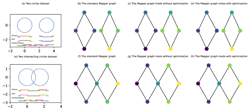
Figure 2: Comparison of the standard Mapper algorithm and our proposed algorithm on a two disjoint circles dataset and a two intersecting circles dataset. (a, e). A visualization of the datasets. Coloured lines represents the intervals produced by each algorithm. (b, f). Output graphs of the standard Mapper algorithm with $n=6,p=0.33$ for the two disjoint circles and $n=5,p=0.2$ for the two intersecting circles. (c, g). The output Mapper graph mode of our proposed method without optimization. (d, h). The output Mapper graph mode of our proposed method with optimization.

We make slight modifications to the datasets above, resulting in two disjoint and two intersecting circles with different radius, each containing $1000$ points. The filter function remains the $x$-axis coordinates. For the unequal-sized disjoint circles, DBSCAN parameters are set to $\epsilon=0.3$ and $minPts=5$; for the unequal-sized intersecting circles, parameters are $\epsilon=0.2$ and $minPts=5$. The standard Mapper struggles to capture the correct topological structure due to its fixed interval setting, whereas our method can adjust intervals based on data distribution, facilitating the accurate capture of the data’s underlying shape. In the case of the unequal-sized intersecting circles dataset, the Mapper graph mode fails to correctly capture the data structure without optimization. However, with optimization, the intervals are slightly adjusted, leading to accurate results.

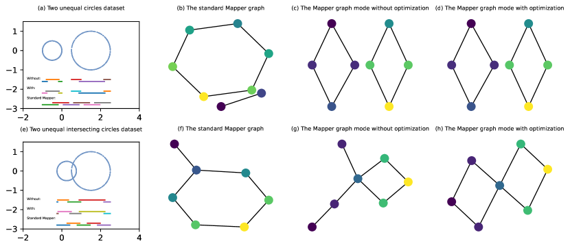
Figure 3: Comparison of the standard Mapper algorithm and our proposed algorithm on a two unequal-sized disjoint circles dataset and a two unequal-sized intersecting circles dataset. (a, e). A visualization of the datasets. Coloured lines represents the intervals produced by each algorithm. (b, f). Output graphs of the standard Mapper algorithm with $n=6,p=0.1$ for the disjoint circles and $n=5,p=0.2$ for the intersecting circles. (c, g). The output Mapper graph mode of our proposed method without optimization. (d, h). The output Mapper graph mode of our proposed method with optimization.

4.2 Noisy dataset

In this section, we assess the robustness of our proposed algorithm by introducing noises into the intersecting circles dataset. The noise is drawn from a Gaussian distribution and is added to each point’s coordinates. Initially, we introduce a small amount of noise, characterized by a Gaussian distribution with mean of zero and standard deviation of $0.1$. The dataset is shown in Figure 4 (a). With this setting for noises, both the standard Mapper and our Mapper graph mode can accurately represent the correct topological structure. The results are shown in Figure 4 (b)-(d).

Subsequently, we increase the noise level, increasing the standard deviation up to $0.3$. At this noise level, the standard Mapper algorithm is unable to output meaningful structures, as illustrated in Figure 4 (f). Conversely, after optimization, our Mapper graph mode still can capture the two primary loops, as shown in Figure 4 (h), though with some additional branches and isolated points. These results highlight the efficacy of flexible interval partitioning in uncovering the data’s inherent structure, even in the presence of significant noise. Parameter optimization plays a crucial role in accurately determining the intervals, which boosts the algorithm’s performance.

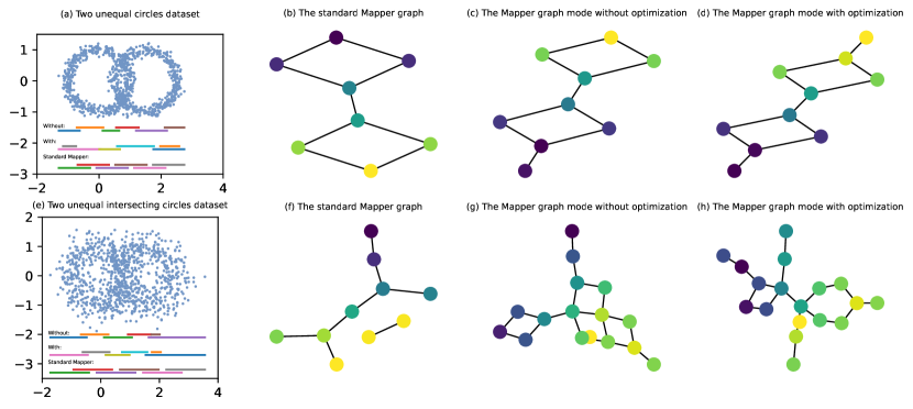
Figure 4: Comparison of the standard Mapper algorithm and our proposed algorithm on a two intersecting circles dataset with noises. (a, e). A visualization of the datasets. Coloured lines represents the intervals produced by each algorithm. (b, f). Output graphs of the standard Mapper algorithm with $n=6,p=0.4$ for the disjoint circles and $n=6,p=0.4$ for the intersecting circles. (c, g). The output Mapper graph mode of our proposed method without optimization. (d, h). The output Mapper graph mode of our proposed method with optimization.

4.3 3D human dataset

We finally test our proposed algorithm on a 3D human dataset from Oulhaj et al. (2024). In this example, the number of intervals is set to $K=8$ and the DBSCAN clustering with parameters $\epsilon=0.6,minPts=5$ is used. The filter function is the mean value of distance between each sample and others. The Mapper graph mode, initialized with an appropriate choice for the GMM parammeters, captures the topological structure better than the standard Mapper graph as shown in Figure 5. After optimization, the Mapper graph mode shows a more concise structure. These results indicates that the proposed soft Mapper algorithm performs better than the standard Mapper concerning the visualization of topological structures, and the optimization process successfully further optimize the topological structures.

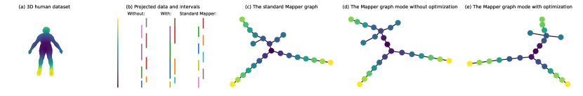
Figure 5: Comparison of the standard Mapper algorithm and our proposed algorithm on a 3D human dataset. (a) A visualization of the 3D human dataset. (b) The projected data and resulted intervals of each algorithm. (c) The output graph of the standard Mapper algorithm, the number of intervals is $8$ and the overlap rate is $0.1$. (d) The Mapper graph mode without optimization. (e) The Mapper graph mode with optimization.

Table 1: Model parameters setting for synthetic datasets

Dataset	$K$	clustering	learning rate	N
Two disjoint circles	6	DBSCAN(0.6,5)	0.005	200
Two unequal disjoint circles	6	DBSCAN(0.3,5)	0.001	300
Two intersecting circles	5	DBSCAN(0.6,5)	0.01	100
Two unequal intersecting circles	5	DBSCAN(0.2,5)	0.001	400
Two intersecting circles with noise	6	DBSCAN(0.2,5)	0.002	300
3D human	8	DBSCAN(0.1,5)	0.0001	350

5 Application

We also apply our method to an RNA expression dataset to assess its ability to identify subgroups within Alzheimer’s disease (AD) patients. The dataset is obtained from the Mount Sinai/JJ Peters VA Medical Center Brain Bank (MSBB) (Wang et al., 2018), which includes RNA gene expression profiles from four distinct brain regions, the frontal pole (FP) in Brodmann area 10, the superior temporal gyrus (STG) in area 22, the parahippocampal gyrus (PHG) in area 36, and the inferior frontal gyrus (IFG) in area 44. In this application study, we focus on brain area 36, which includes $215$ patient samples, each with over $20,000$ gene expression values. Each patient is given a Braak AD staging score, ranging from $0$ to $6$, with higher scores indicating more severe disease stages (Braak et al., 2003). The Braak score is treated as a label for each sample. Our goal is to identify subgroups with a significantly different distribution of Braak scores from the rest of the population given the gene expression profiles. These subgroups can be branches or isolated nodes on the hidden topological features of the gene expression profiles.

As indicated in Zhou and Sharpee (2021), the gene expression data could exhibit a hyperbolic structure especially as the number of genetic sites increases . To capture the complex and hierarchical relationships between samples based on gene expression more effectively, we use the Lorentzian distance, a standard hyperbolic distance, to measure the similarity between samples. The hyperbolic distance can preserve the hierarchical structures inherent in gene expression data and is considered particularly suitable for high-dimensional data (Liu et al., 2024). In the Lorentzian distance, the centroid is crucial due to its ability to reveal the hierarchical structure of datasets. In this study, we set each data point in the dataset as the centroid to get a distance matrix repetitively and use the averaged distance matrix as the final distance matrix. The filter function is set to the mean value of distance between each sample and others. Due to the high computational cost of calculating the distance matrix for over $20,000$ genes, we select the top $37$ gene sites as listed in Wang et al. (2016). These gene sites are from the top $50$ probes ranked in association with disease traits across $19$ brain regions, excluding those unmatched. The selected gene sites are then used to compute the hyperbolic distances.

We set the number of intervals to $n=15$, the learning rate to $\gamma=0.001$, and the number of epochs to $N=300$. We apply agglomerative clustering with a threshold of $3.13$ (Müllner, 2011). Additionally, we initialize the parameters by fitting a Gaussian mixture model to the projected data. The graph modes of the GMM soft Mapper algorihtm without and with optimation is given in Appendix C. Training loss of the GMM soft Mapper while optimizing prameter is given in the Appendix D. The resulting optimized Mapper graph mode offers valuable insights into Alzheimer’s disease progression. The $\chi^{2}$ test is used to determine if there is a statistically significant difference between the distribution of the identified subgroup and the rest of the population (Mannan and Meslow, 1984).

In brain area 36, we find a distinct branch which is associated with high Braak scores, as shown in the red dashed box in Figure 6 (a). The bar charts in Figure 6 (b) reveals distribution differences between this branch and the rest nodes. The $P-$value of the $\chi^{2}$ test is $0.0047$, less than $0.05$, indicating a significant difference in distribution. $73\%$ of patients in this unique group have severe Alzheimer’s disease, while the averaged ratio in the rest nodes is $37\%$. This indicates that the gene expression patterns in this cohort differ from the rest, and merit further investigation.

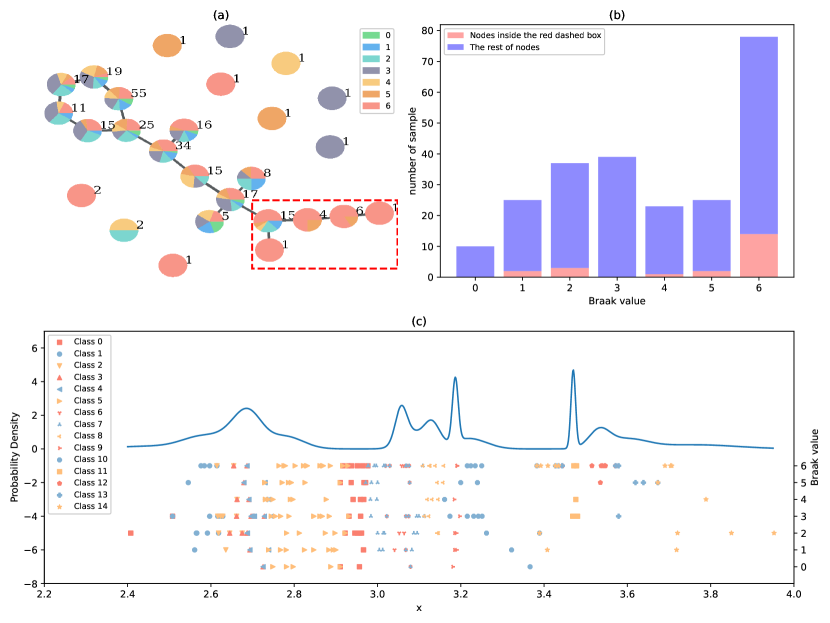
Figure 6: Results of the brain area 36. (a) The output Mapper graph mode of a GMM soft Mapper with optimization. The pie charts at each node illustrate the distribution of Braak scores within this node, with the number next to each node representing the sample size in the node. Nodes within the red dashed box is a cluster that exhibits a distinct distribution compared to samples in the rest nodes. (b) The bar chart compares the distribution of Braak scores of the nodes within the red dashed box to those of the rest nodes. (c) A visualization of the projected data along with the optimized GMM probability density. In this figure, the values of the major $y$-axis represent the GMM density and the values of the minor $y$-axis represent the Braak scores of each data point. Coloured markers signify the various implicit intervals to which a point belongs.

6 Discussion

In this work, we introduce a novel approach for flexibly constructing a Mapper graph based on a probability model. We develop implicit intervals for soft Mapper graphs using a Gaussian mixture model and a multinomial distribution. With a given number of intervals, our algorithm automatically assigns each data point to an interval based on the allocation probability. Then based on these implicit intervals, we derive the concept of the Mapper graph mode as a point estimation. Additionally, we design an optimization approach that enhances the topological structure of Mapper graphs by minimizing a specific loss function. This function considers both the likelihood of the projected data with respect to the GMM and the topological information of the Mapper graph mode. This optimization process is particularly suited for complex and noisy datasets, as the standard Mapper algorithm can be sensitive to noise and may fail in certain situations. Both simulation and application studies demonstrate its effectiveness in capturing the underlying topological structures. The application of our proposed algorithm to gene expression of brain area 36 from the MSBB successfully identifies a unique subgroup whose distribution of Braak scores significantly differs from the rest of the nodes.

It is worth noting that the multimodal nature of the objective function makes it challenging to find a globally optimal Mapper graph. Careful parameter tuning and domain expertise are essential for generating a high quality Mapper graph. In addtion, the mean persistence loss function used in this work is a simple representation of information on the extended persistence diagram. Numerous alternative approaches may be available, for instance, one could consider distinguishing signals from noise in a Mapper graph using confidence sets (Fasy et al., 2013). Finding a more robust persistence-specific loss function will be a one of the furtur work directions. Morevoer, as you may have noticed, the filter function is also important for constructing a meaningful Mapper graph, in this work, covers are directly constructed on filtered data first, as most literture does. Optimizing the filter function and intervals simultaneously would be a challenging but meanfully direction.

Appendix A. Theoretical derivation of the mode of a mutilnomial distribution

Suppose $(h_{1},..,h_{K})$ follows a multinomial distribution with total event number $m=2$,

$$(h_{1},..,h_{K})\sim{Multi}(2,q_{1},..,q_{K}).$$

Then the probability density function of $(h_{1},..,h_{K})$ is

$$p(h_{1},..,h_{K})=\frac{2}{h_{1}!h_{2}!...h_{n}!}q_{1}^{h_{1}}q_{2}^{h_{2}}...q_{K}^{h_{K}}.$$

To compute the mode of a Mutilnomial distribution, i.e.,

$$\mathop{\arg\max}\limits_{(h_{1},..,h_{K})}p(h_{1},..,h_{K})=\mathop{\arg\max}\limits_{(h_{1},..,h_{K})}\frac{2}{h_{1}!h_{2}!...h_{n}!}q_{1}^{h_{1}}q_{2}^{h_{2}}...q_{K}^{h_{K}}.$$

When the total event number $m=2$, the possible values of $(h_{1},..,h_{K})$ can be divided into two following cases.

Case 1. Two elements of $(h_{1},..,h_{K})$ are $1$ and others are $0$.

In this case, to get the maximum probability, denote $q^{*}=max(q_{1},q_{2},...q_{K})$ the largest probability and $q^{**}=max\{q_{1},q_{2},...q_{K}\}\setminus\{q^{*}\}$ the second largest probability among $\{q_{1},q_{2},...q_{K}\}$. $i^{*}$ and $i^{**}$ represent the index of $q^{*}$ and $q^{**}$. Therefore, we have $h_{i^{*}}=h_{i^{**}}=1$ and others to zero. The probability of this case is

$$\mathop{\arg\max}\limits_{(h_{1},..,h_{K})}\frac{2}{h_{1}!h_{2}!...h_{n}!}q_{1}^{h_{1}}q_{2}^{h_{2}}...q_{K}^{h_{K}}=2q^{*}q^{**}.$$

Case 2. One element of $(h_{1},..,h_{K})$ is $2$ and others are $0$.

In this case, we have $h_{i^{*}}=2$ and others to zero. The probability of this case is

$$\mathop{\arg\max}\limits_{(h_{1},..,h_{K})}\frac{2}{h_{1}!h_{2}!...h_{n}!}q_{1}^{h_{1}}q_{2}^{h_{2}}...q_{K}^{h_{K}}=(q^{*})^{2}.$$

Therefore, to get the mode of a multinomial distribution with $m=2$, we only need to consider the following two situations.

If $\frac{1}{2}q^{*}>q^{**}$,

$$h_{mode}(i)=\begin{cases}2&\text{if }i=i^{*},\\ 0&\text{otherwise}.\end{cases}$$

If $\frac{1}{2}q^{*}\leq q^{**}$,

$$h_{mode}(i)=\begin{cases}1&\text{if }i=i^{*},i^{**},\\ 0&\text{otherwise}.\end{cases}$$

Appendix B. Samples from the optimized GMM soft Mapper of synthetic datasets

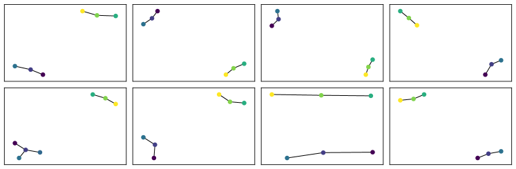
Figure 7: Eight samples from the optimized GMM soft Mapper of the two disjoint circles dataset.

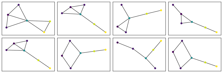
Figure 8: Eight samples from the optimized GMM soft Mapper of the two intersecting circles dataset.

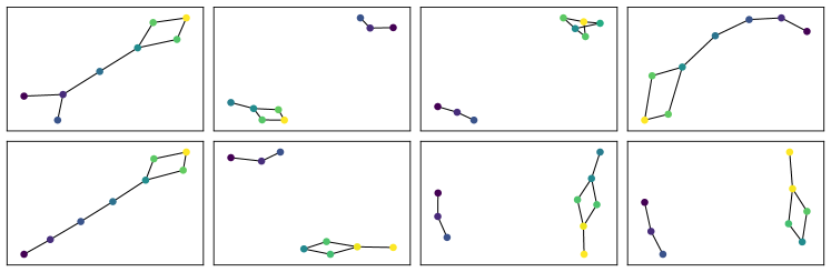
Figure 9: Eight samples from the optimized GMM soft Mapper of the two disjoint circles with different radius dataset.

Figure 10: Eight samples from the optimized GMM soft Mapper of the two intersecting circles with different radius dataset.

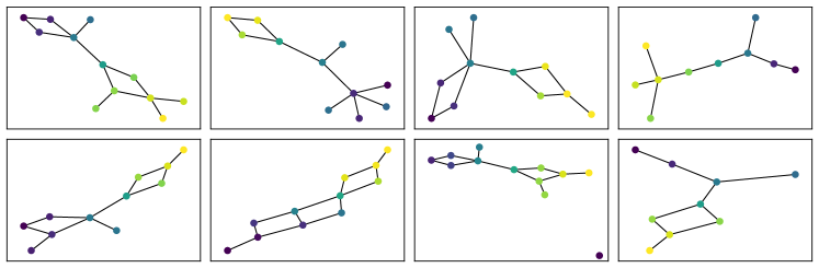
Figure 11: Eight samples from the optimized GMM soft Mapper of the two circles with small noise dataset.

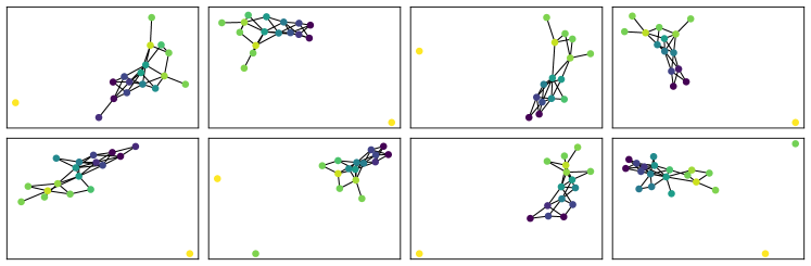
Figure 12: Eight samples from the optimized GMM soft Mapper of the two intersecting circles with big noise dataset.

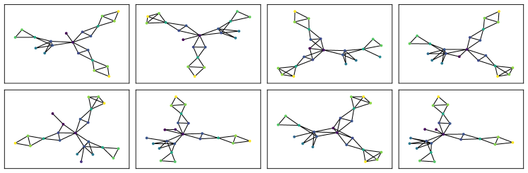
Figure 13: Eight samples from the optimized GMM soft Mapper on the 3D human dataset.

Appendix C. The GMM soft Mapper modes for brain area 36

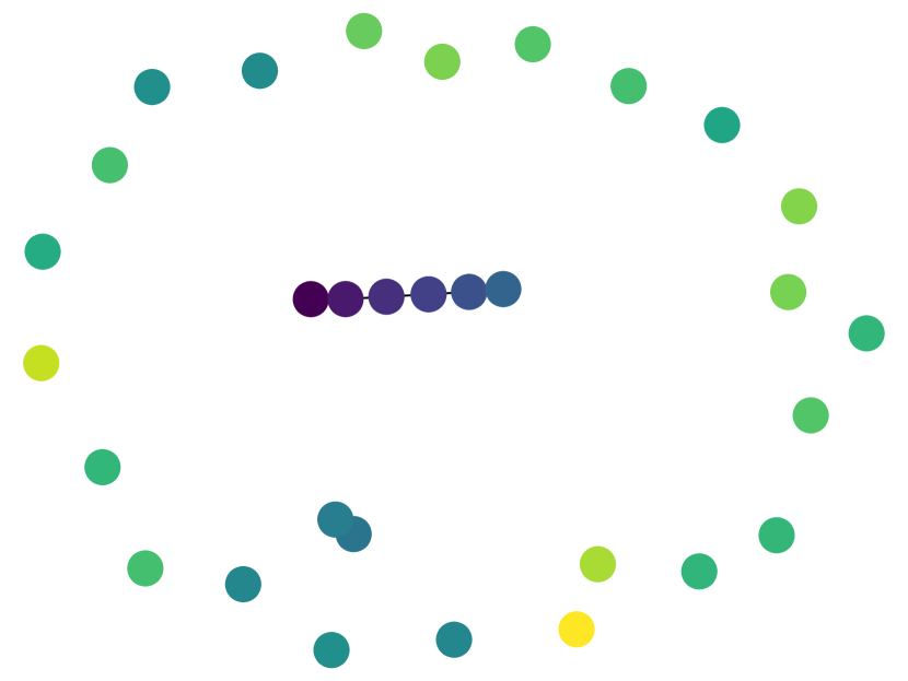
Figure 14: The graph mode of the GMM soft Mapper without optimization for brain area 36.

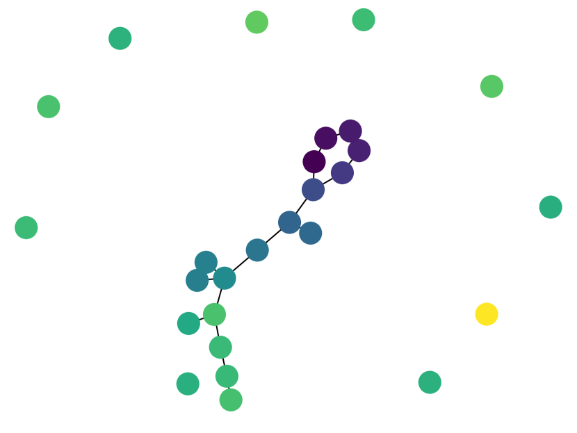
Figure 15: The graph mode of the GMM soft Mapper with optimization for brain area 36.

Appendix D. Loss figures

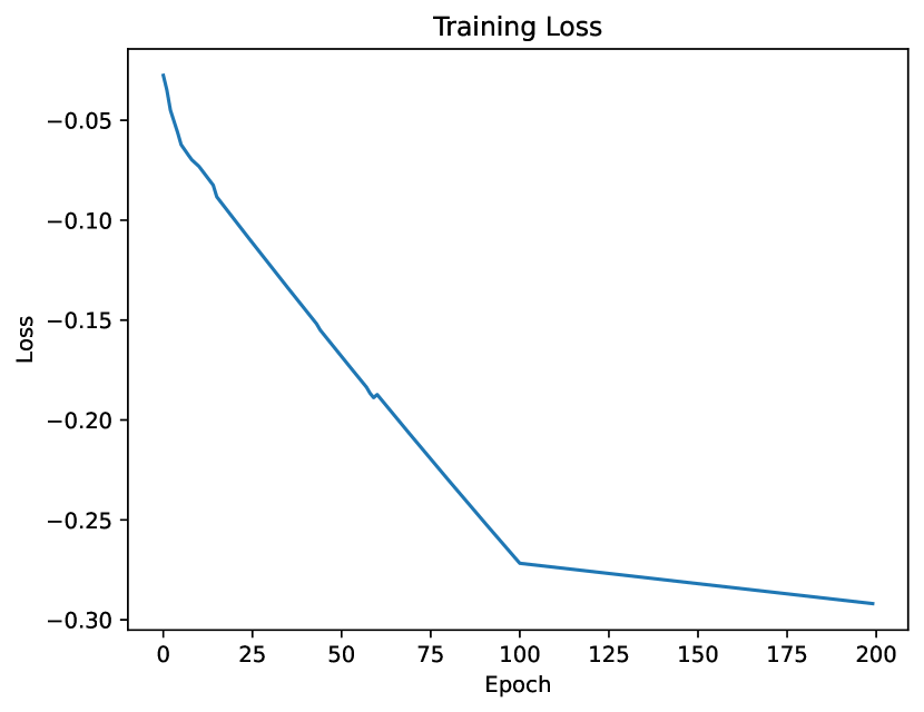
(a)

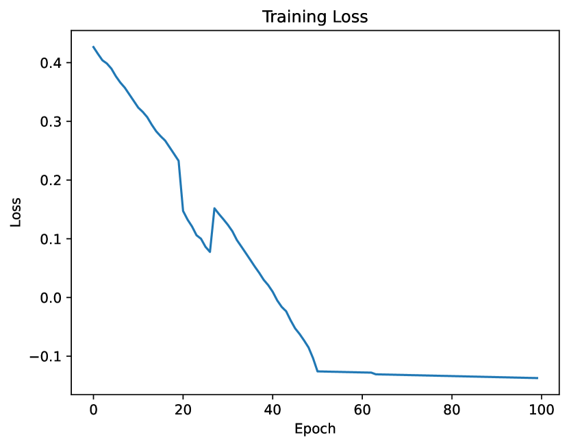
(b)

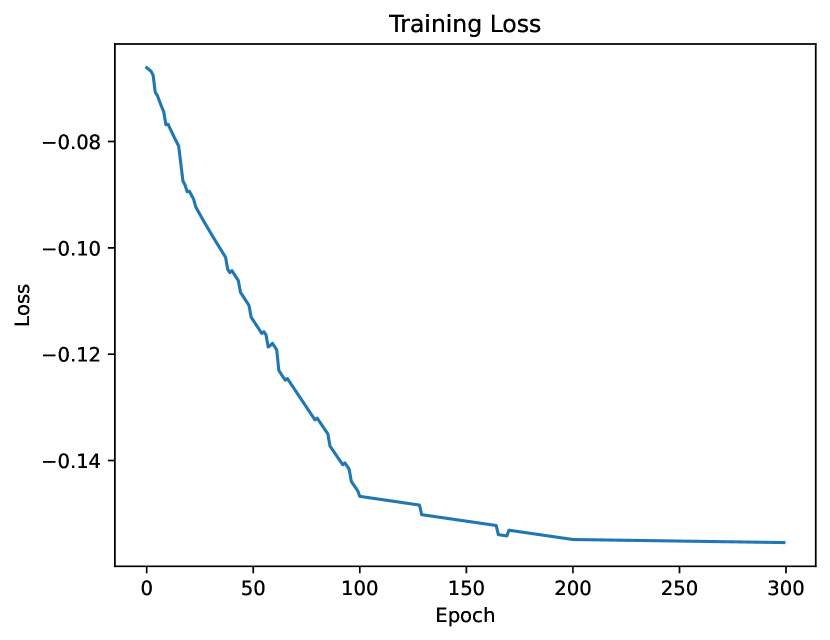
(c)

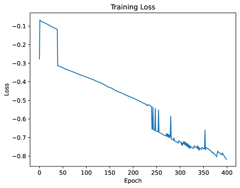
(d)

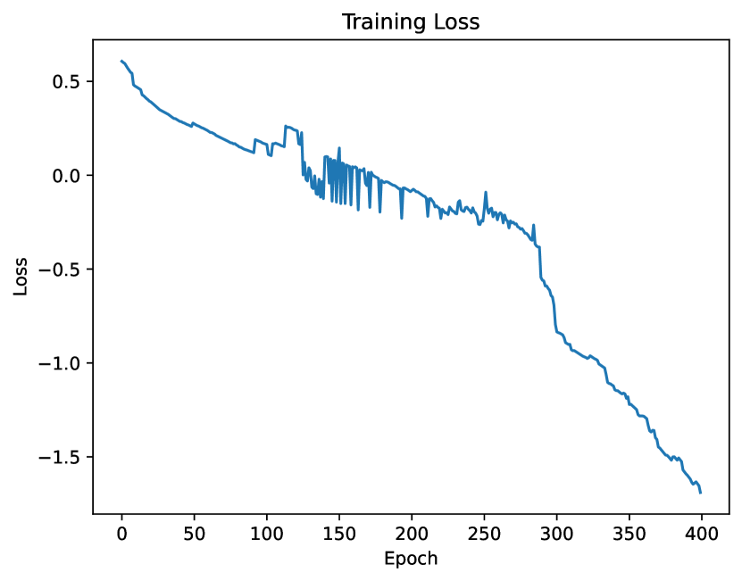
(e)

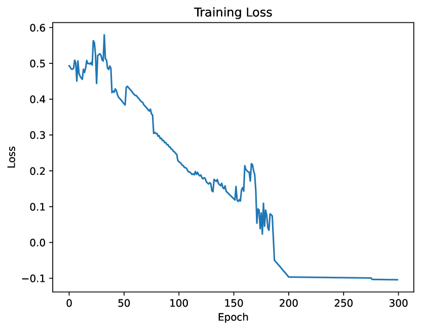
(f)

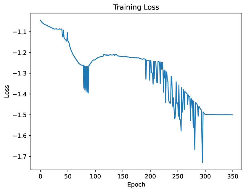
(g)

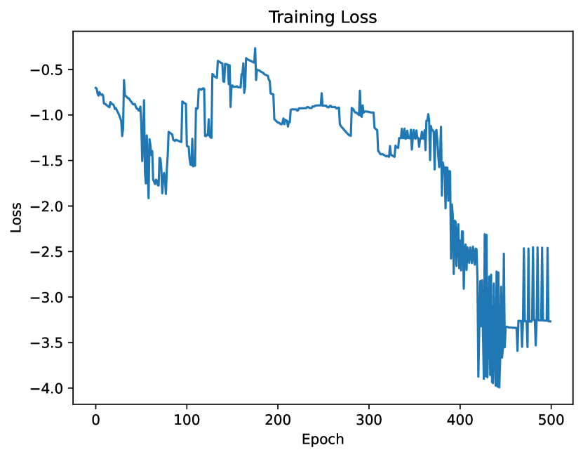
(h)

Figure 16: Training loss of the GMM soft Mapper while optimizing prameter for each dataset. (a). Dataset of the two disjoint circles. (b) Dataset of the two intersecting circles. (c) Dataset of the two circles with different radius. (d) Dateset of the two intersecting circles with different radius. (e) Dataset of the two intersecting circles with small noises. (f) Dataset of the two intersecting circles with large noises. (g) The 3D human dataset. (h) Brain area 36 dataset.

References

- Abadi et al. (2016) Abadi, M., Barham, P., Chen, J., Chen, Z., Davis, A., Dean, J., Devin, M., Ghemawat, S., Irving, G., Isard, M., Kudlur, M., Levenberg, J., Monga, R., Moore, S., Murray, D. G., Steiner, B., Tucker, P., Vasudevan, V., Warden, P., Wicke, M., Yu, Y., and Zheng, X. Tensorflow: A system for large-scale machine learning, 2016. URL https://arxiv.org/abs/1605.08695.
- Bauer et al. (2024) Bauer, U., Botnan, M. B., and Fluhr, B. Universal distances for extended persistence. Journal of Applied and Computational Topology, Jul 2024. ISSN 2367-1734. 10.1007/s41468-024-00184-7. URL https://doi.org/10.1007/s41468-024-00184-7.
- Bodnar et al. (2021) Bodnar, C., Cangea, C., and Liò, P. Deep Graph Mapper: Seeing Graphs Through the Neural Lens. Frontiers in Big Data, 4, 2021. ISSN 2624-909X.
- Bottou (2010) Bottou, L. Large-scale machine learning with stochastic gradient descent. In Lechevallier, Y. and Saporta, G., editors, Proceedings of COMPSTAT’2010, pages 177–186, Heidelberg, 2010. Physica-Verlag HD. ISBN 978-3-7908-2604-3.
- Braak et al. (2003) Braak, H., Del Tredici, K., Rüb, U., De Vos, R. A., Steur, E. N. J., and Braak, E. Staging of brain pathology related to sporadic parkinson’s disease. Neurobiology of aging, 24(2):197–211, 2003.
- Brown et al. (2021) Brown, A., Bobrowski, O., Munch, E., and Wang, B. Probabilistic convergence and stability of random mapper graphs. J Appl. and Comput. Topology, 5(1):99–140, March 2021. ISSN 2367-1734. 10.1007/s41468-020-00063-x.
- Bubenik (2015) Bubenik, P. Statistical topological data analysis using persistence landscapes. The Journal of Machine Learning Research, 16(1):77–102, January 2015. ISSN 1532-4435.
- Bui et al. (2020) Bui, Q.-T., Vo, B., Do, H.-A. N., Hung, N. Q. V., and Snasel, V. F-Mapper: A Fuzzy Mapper clustering algorithm. Knowledge-Based Systems, 189:105107, February 2020. ISSN 09507051. 10.1016/j.knosys.2019.105107.
- Carrière and Oudot (2018) Carrière, M. and Oudot, S. Structure and Stability of the One-Dimensional Mapper. Found Comput Math, 18(6):1333–1396, December 2018. ISSN 1615-3383. 10.1007/s10208-017-9370-z.
- Carrière et al. (2018) Carrière, M., Michel, B., and Oudot, S. Statistical analysis and parameter selection for mapper. J. Mach. Learn. Res., 19(1):478–516, January 2018. ISSN 1532-4435.
- Cyranka et al. (2019) Cyranka, J., Georges, A., and Meyer, D. Mapper Based Classifier. In 2019 18th IEEE International Conference On Machine Learning And Applications (ICMLA), pages 1099–1106, December 2019. 10.1109/ICMLA.2019.00184.
- Dey et al. (2017) Dey, T. K., Mémoli, F., and Wang, Y. Topological Analysis of Nerves, Reeb Spaces, Mappers, and Multiscale Mappers. page 16 pages, Wadern/Saarbruecken, Germany, 2017. Schloss Dagstuhl - Leibniz-Zentrum fuer Informatik GmbH. 10.4230/LIPICS.SOCG.2017.36. URL http://drops.dagstuhl.de/opus/volltexte/2017/7222/. Artwork Size: 16 pages Medium: application/pdf.
- Dłotko (2019) Dłotko, P. Ball mapper: A shape summary for topological data analysis, January 2019.
- Fasy et al. (2013) Fasy, B. T., Lecci, F., Rinaldo, A., Wasserman, L., Balakrishnan, S., and Singh, A. Confidence sets for persistence diagrams. Computer Science, 42(6):2301–2339, 2013.
- Fitzpatrick et al. (2023) Fitzpatrick, P., Jurek-Loughrey, A., Dłotko, P., and Rincon, J. M. D. Ensemble Learning for Mapper Parameter Optimization. In 2023 IEEE 35th International Conference on Tools with Artificial Intelligence (ICTAI), pages 129–134, November 2023. 10.1109/ICTAI59109.2023.00026.
- Gepperth and Pfülb (2021) Gepperth, A. and Pfülb, B. Gradient-Based Training of Gaussian Mixture Models for High-Dimensional Streaming Data. Neural Process Lett, 53(6):4331–4348, December 2021. ISSN 1573-773X. 10.1007/s11063-021-10599-3.
- Kamruzzaman et al. (2021) Kamruzzaman, M., Kalyanaraman, A., Krishnamoorthy, B., Hey, S., and Schnable, P. S. Hyppo-X: A Scalable Exploratory Framework for Analyzing Complex Phenomics Data. IEEE/ACM Transactions on Computational Biology and Bioinformatics, 18(4):1535–1548, July 2021. ISSN 1557-9964. 10.1109/TCBB.2019.2947500.
- Kang and Lim (2021) Kang, S. J. and Lim, Y. Ensemble mapper. Stat, 10(1), December 2021. ISSN 2049-1573, 2049-1573. 10.1002/sta4.405.
- Kumari et al. (2020) Kumari, N., R., S., Rupela, A., Gupta, P., and Krishnamurthy, B. Shapevis: High-dimensional data visualization at scale. In Proceedings of The Web Conference 2020, WWW ’20, page 2920–2926, New York, NY, USA, 2020. Association for Computing Machinery. ISBN 9781450370233. 10.1145/3366423.3380058. URL https://doi.org/10.1145/3366423.3380058.
- Liu et al. (2024) Liu, B., Lubold, S., Raftery, A. E., and McCormick, T. H. Bayesian hyperbolic multidimensional scaling. Journal of Computational and Graphical Statistics, pages 1–14, 2024. 10.1080/10618600.2024.2308219. URL https://doi.org/10.1080/10618600.2024.2308219.
- Mannan and Meslow (1984) Mannan, R. W. and Meslow, E. C. Bird populations and vegetation characteristics in managed and old-growth forests, northeastern oregon. The Journal of wildlife management, pages 1219–1238, 1984.
- Müllner (2011) Müllner, D. Modern hierarchical, agglomerative clustering algorithms. arXiv preprint arXiv:1109.2378, 2011.
- Nicolau et al. (2011) Nicolau, M., Levine, A. J., and Carlsson, G. Topology based data analysis identifies a subgroup of breast cancers with a unique mutational profile and excellent survival. Proceedings of the National Academy of Sciences, 108(17):7265–7270, April 2011. ISSN 0027-8424, 1091-6490. 10.1073/pnas.1102826108. URL https://pnas.org/doi/full/10.1073/pnas.1102826108.
- Oulhaj et al. (2024) Oulhaj, Z., Carrière, M., and Michel, B. Differentiable Mapper For Topological Optimization Of Data Representation, February 2024. URL http://arxiv.org/abs/2402.12854. arXiv:2402.12854 [cs, math].
- Paszke et al. (2019) Paszke, A., Gross, S., Massa, F., Lerer, A., Bradbury, J., Chanan, G., Killeen, T., Lin, Z., Gimelshein, N., Antiga, L., Desmaison, A., Köpf, A., Yang, E., DeVito, Z., Raison, M., Tejani, A., Chilamkurthy, S., Steiner, B., Fang, L., Bai, J., and Chintala, S. Pytorch: An imperative style, high-performance deep learning library, 2019. URL https://arxiv.org/abs/1912.01703.
- Rizvi et al. (2017) Rizvi, A. H., Camara, P. G., Kandror, E. K., Roberts, T. J., Schieren, I., Maniatis, T., and Rabadan, R. Single-cell topological RNA-seq analysis reveals insights into cellular differentiation and development. Nat Biotechnol, 35(6):551–560, June 2017. ISSN 1087-0156, 1546-1696. 10.1038/nbt.3854.
- Schubert et al. (2017) Schubert, E., Sander, J., Ester, M., Kriegel, H. P., and Xu, X. Dbscan revisited, revisited: Why and how you should (still) use dbscan. ACM Trans. Database Syst., 42(3), July 2017. ISSN 0362-5915. 10.1145/3068335. URL https://doi.org/10.1145/3068335.
- Singh et al. (2007) Singh, G., Memoli, F., and Carlsson, G. Topological Methods for the Analysis of High Dimensional Data Sets and 3D Object Recognition. In Botsch, M., Pajarola, R., Chen, B., and Zwicker, M., editors, Eurographics Symposium on Point-Based Graphics, The Netherlands., 2007. The Eurographics Association. 10.2312/SPBG/SPBG07/091-100.
- Skaf and Laubenbacher (2022) Skaf, Y. and Laubenbacher, R. Topological data analysis in biomedicine: A review. Journal of Biomedical Informatics, 130:104082, June 2022. ISSN 15320464. 10.1016/j.jbi.2022.104082.
- Tao and Ge (2024) Tao, Y. and Ge, S. A distribution-guided mapper algorithm. arXiv preprint arXiv:2401.12237, 2024.
- Wang et al. (2016) Wang, M., Roussos, P., McKenzie, A., Zhou, X., Kajiwara, Y., Brennand, K. J., De Luca, G. C., Crary, J. F., Casaccia, P., Buxbaum, J. D., et al. Integrative network analysis of nineteen brain regions identifies molecular signatures and networks underlying selective regional vulnerability to alzheimer’s disease. Genome medicine, 8:1–21, 2016.
- Wang et al. (2018) Wang, M., Beckmann, N. D., Roussos, P., Wang, E., Zhou, X., Wang, Q., Ming, C., Neff, R., Ma, W., Fullard, J. F., et al. The mount sinai cohort of large-scale genomic, transcriptomic and proteomic data in alzheimer’s disease. Scientific data, 5(1):1–16, 2018. https://doi.org/10.1038/sdata.2018.185.
- Zhou and Sharpee (2021) Zhou, Y. and Sharpee, T. O. Hyperbolic geometry of gene expression. iScience, 24(3), Mar 2021. ISSN 2589-0042. 10.1016/j.isci.2021.102225. URL https://doi.org/10.1016/j.isci.2021.102225.