Quasi-geodesics in integrable and non-integrable exclusion processes

Patrik L. Ferrari Institute for Applied Mathematics, Bonn University, Endenicher Allee 60, 53115 Bonn, Germany. E-mail: ferrari@uni-bonn.de    Min Liu Institute for Applied Mathematics, Bonn University, Endenicher Allee 60, 53115 Bonn, Germany. E-mail: mliu@uni-bonn.de
(January 7, 2025)
Abstract

Backwards geodesics for TASEP were introduced in [26]. We consider flat initial conditions and show that under proper scaling its end-point converges to maximizer argument of the Airy2 process minus a parabola. We generalize its definition to generic non-integrable models including ASEP and speed changed ASEP (call it quasi-geodesics). We numerically verify that its end-point is universal, where the scaling coefficients are analytically computed through the KPZ scaling theory.

1 Introduction

We consider interacting particle systems in the Kardar-Parisi-Zhang (KPZ) universality class, with particle configurations $\eta\in\{0,1\}^{\mathbb{Z}}$, where $\eta(x)=1$ whenever there is a particle at site $x$. A particle at site $x$ jumps to a free site $y$ with jump rate given by a local function $c_{\eta}(x,y)$. In this paper we consider three variants of exclusion processes with nearest-neighbor jumps, namely the totally asymmetric simple exclusion process (TASEP), the partially asymmetric simple exclusion process (ASEP), and the speed changed ASEP (ASEPsc). In the latter the function $c_{\eta}(x,x+1)$ and $c_{\eta}(x+1,x)$ depend on $\eta(x-1)$ and $\eta(x+2)$ as well. While TASEP can be analyzed with exact formulas, and partially it is also the case for ASEP, the speed changed ASEP considered here is non-integrable with known stationary measures [40], allowing us to analytically compute all non-universal coefficients for the KPZ scaling theory [54, 46].

Since jumps are nearest-neighbor, the particle ordering is maintained. We label particles from right to left and call $X_{n}(t)$ the position of particle $n$ at time $t$. One way to see this model as a growing interface is to consider $n\mapsto X_{n}(t)+n$ as height function. This is a rotation by 45 degrees of the (more standard) height function whose gradient is given by $1-2\eta(x)$.

As the KPZ universality class has $1:2:3$ scaling, fluctuations of the interface grow as $t^{1/3}$ and space-time correlations are non-trivial in a $t^{2/3}$-neighborhood of characteristic lines. In analogy to last passage percolation (LPP) models (and its universal scaling limit, the directed landscape ${\cal L}$ [23]), one can define a notion of geodesics: for a given $(N,t)$, any trajectory $(X_{N(\tau)}(\tau))_{\tau:t\to 0}$ satisfying the concatenation property

$$X_{N}(t)=X_{N(\tau)}(\tau)+X^{{\rm step}}_{N-{N(\tau)}}(\tau,t),$$ (1.1)

where $X^{{\rm step}}_{N-{N(\tau)}}(\tau,t)$ is the position of the particle number $N-{N(\tau)}$ of TASEP which starts at time $\tau$ with particles occupying all sites to the left of $X_{N(\tau)}(\tau)$. The reason we call it (backwards) geodesics, is in [52] it was shown that

$$X_{N}(t)=\min_{M\leq N}\left\{X_{M}(\tau)+X^{{\rm step}}_{N-M}(\tau,t)\right\},$$ (1.2)

so along these paths the minimization (1.2) is fulfilled.

Geodesics have attracted a lot of interest and many properties have been studied, mostly in the framework of LPP (see e.g. [18, 11, 58, 45, 5, 8, 4, 10, 38]), but also in the scaling limit of the directed landscape (see e.g. [19, 12, 22, 24, 49]). Properties of geodesics, in particular of localization, have also been very important to study other observables, like the decay of the covariance in the Airy1 process [6], the universality of first order correction of the time-time covariance [33, 34, 7, 9], the analysis of mixing times [51], but also the height function in presence of shocks without passing through maps to LPP [17, 30, 15, 28, 31].

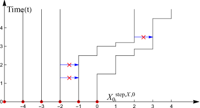
In [26] a dynamical construction of a backwards geodesic was proposed. In short, the geodesic follows backwards the trajectory of a particle (starting with particle $N$ at time $t$) and every time the particle on the geodesics is prevented from jumping, it follows the backwards trajectory of the blocking particle. This construction is natural since it keeps track of which regions in space-time actually influenced the position of particle $N$ at time $t$, $X_{N}(t)$. In particular, if we know that the backwards geodesics is in a given space-time non-random region $D$ (with high probability), then the position $X_{N}(t)$ is independent of the randomness outside the region $D$ (see Lemma 3.1 of [28] for an explicit statement).

The main goal of this work is to investigate whether the generalization of the dynamical construction of backwards geodesics applied to non- or partially-integrable systems such as speed changed ASEP or ASEP is universal. For these models (1.1) is no longer satisfied, but as proven for ASEP [48] the height functions converge in the scaling limit to the KPZ fixed point, for which

$$h(x,t)=\max_{y\in\mathbb{R}}\{h(y,0)+{\cal L}(y,0;x,t)\}.$$ (1.3)

By universality we expect the same to be true for speed changed ASEP and we call our physically motivated generalization quasi-geodesics.

For our study we consider flat initial condition (with density $1/2$), that is, $X_{N}(0)=-2N$ for $N\in\mathbb{Z}$. First of all, we prove for TASEP in Theorem 2.19 that the end-point of the backwards geodesics, $x_{N(0)}(0)$, in the $t^{2/3}$ scale, has a limit law given by the $\operatorname*{argmax}_{u\in\mathbb{R}}\{{\cal A}_{2}(u)-u^{2}\}$, where ${\cal A}_{2}$ is the Airy2 process [47]. The analogue result for line-to-point exponential LPP can be found in [50, 3].

To verify the universality conjecture, we first need to derive precise conjectures based on the scaling from the KPZ scaling theory, see Section 3.2: all the non-universal model-dependent parameters are computed analytically allowing us to formulate precise conjectures for the end-point of the quasi-geodesics without free parameters, see Conjecture 2.7 for ASEP and Conjecture 2.8 for speed changed ASEP. In Section 4 we provide numerical evidence that these conjectures hold true.

For the speed changed ASEP, we also verify that with flat initial condition the one-point distribution is asymptotically given by the GOE Tracy-Widom distribution as expected by universality, see Section 4.2.1.

Finally, as mentioned above, for ASEP it is known that (1.2) is only an inequality (see e.g. [17, 30]). From the results of [48] it follows that the difference

$$\min_{M\leq N}\left\{X_{M}(\tau)+X^{{\rm step}}_{N-M}(\tau,t)\right\}-X_{N}(t)\geq 0,$$ (1.4)

once divided by $t^{1/3}$, goes to zero as $t\to\infty$ (see Lemma 2.10). However the speed of convergence to zero remains unknown. For that reason, using our quasi-geodesic, we numerically study the discrepancy

$$d(t)=X_{N(\tau)}(\tau)+X^{{\rm step}}_{N-{N(\tau)}}(\tau,t)-X_{N}(t)\geq 0,$$ (1.5)

which clearly is a bound for (1.4). Surprisingly the numerical simulation indicates that $d(t)$ tends to a finite random variable, without the need to be divided by $t^{\theta}$ for some $\theta\in(0,1/3)$, see Section 4.1.2. Thus for ASEP the correction to (1.2) is of order one. In a recent paper [1] it is shown that the height function has bounded discrepancy from the maximum of some LPP line ensembles (see Section 4 of [1]). However, it remains unclear how to relate the entries in the line ensembles with ASEP height functions.

Outline.

We present our results in Section 2. In Section 2.1, we introduce the models ASEP and speed changed ASEP. The generalized backward geodesic is defined in Section 2.2. Analytical results for the backward geodesic in TASEP are given in Section 2.3 and proved later in Section 3.1. The exact scaling formulas for non-integrable models are also provided in Section 2.3, with a detailed explanation on how to use KPZ scaling theory to derive these results given in Section 3.2. Finally, in Section 4, we present numerical results to verify the conjectures mentioned in previous sections.

Acknowledgements:

The work was partly funded by the Deutsche Forschungsgemeinschaft (DFG, German Research Foundation) under Germany’s Excellence Strategy - GZ 2047/1, projekt-id 390685813 and by the Deutsche Forschungsgemeinschaft (DFG, German Research Foundation) - Projektnummer 211504053 - SFB 1060. We authors are grateful to Herbert Spohn for indicating the non-integrable model with computable non-universal scaling coefficients, to Dominik Schmid and Ofer Busani for discussions, as well as Milind Hedge for explaining their approximate LPP representation.

2 Model and results

2.1 Simple exclusion process

The simple exclusion process ($\mathrm{SEP}$) is among the interacting particle systems introduced by Spitzer [53]. It is a Markov process $\eta_{t}$ on configuration space $\Omega=\{0,1\}^{\mathbb{Z}}$ that describes the motion of particles on $\mathbb{Z}$, where $\eta_{t}(i)=1$ (resp. $\eta_{t}(i)=0$) stands for presence (resp. absence) of a particle at position $i$ at time $t$. For a configuration $\eta\in\Omega$ and $x,y\in\mathbb{Z}$, we define $\eta^{x,y}\in\Omega$ as

$$\eta^{x,y}(i)=\begin{cases}\eta(y),\quad&\mathrm{if}\ i=x,\\ \eta(x),&\mathrm{if}\ i=y,\\ \eta(i),&\mathrm{otherwise}.\end{cases}$$ (2.1)

The generator of $\mathrm{SEP}$ is given by

$$\mathcal{L}f(\eta)=\sum_{\begin{subarray}{c}x,y\in\mathbb{Z}\\ |x-y|=1\end{subarray}}c_{\eta}(x,y)\eta(x)(1-\eta(y))(f(\eta^{x,y})-f(\eta))$$ (2.2)

for any cylinder function $f:\Omega\to\mathbb{R}$ and where $c_{\eta}(x,y)$ is the jump rate from site $x$ to site $y$. In this work, we will consider three special cases:

(a) TASEP: The totally asymmetric simple exclusion process (TASEP) has jump rates given by

$$c_{\eta}(x,y)=\begin{cases}1,\quad&\mathrm{if}\ y=x+1,\\ 0,&\mathrm{otherwise}.\end{cases}$$ (2.3)

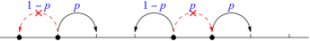
(b) ASEP: The asymmetric simple exclusion process (ASEP) with asymmetry parameter $p\in(1/2,1]$ is defined by the jump rate in (2.2)

$$c_{\eta}(x,y)=\begin{cases}p,\quad&\mathrm{if}\ y=x+1,\\ 1-p,&\mathrm{if}\ y=x-1,\\ 0,&\mathrm{otherwise},\end{cases}$$ (2.4)

see Figure 1 for an illustration.

Refer to caption
Figure 1: Illustration for jump rate in ASEP. In the setting of ASEP, every particle will attempt to jump its nearest neighbour independently with jump rate $p$ to the right and $1-p$ to the left. The attempted jump is successful only if the target site is unoccupied.

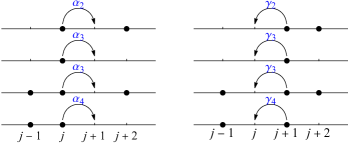
(c) Speed changed ASEP: Speed changed ASEP (ASEPsc) are models where the jump rate is not constant, but it depends on the local particle configuration. We consider here a model with next-nearest-neighbour interactions as in [40]. It is still in the family of SEP since the jumps are nearest-neighbour, that is, for $|i|\geq 2$, $c_{\eta}(x,x+i)=0$. The jump rates from $x$ to $x+1$ and $x-1$ are given as follows. Let $\alpha_{i},\gamma_{i}\geq 0$ with $i\in\{2,3,4\}$ be fixed parameters. Then the right jumps occur with rate

$\displaystyle c_{\eta}(j,j+1)=\begin{cases}\alpha_{2},\quad&\mathrm{if}\ \eta(j-1)=0,\eta(j)=1,\eta(j+1)=0,\eta(j+2)=1,\\ \alpha_{3},\quad&\mathrm{if}\ \eta(j-1)=0,\eta(j)=1,\eta(j+1)=0,\eta(j+2)=0,\\ \alpha_{3},\quad&\mathrm{if}\ \eta(j-1)=1,\eta(j)=1,\eta(j+1)=0,\eta(j+2)=1,\\ \alpha_{4},\quad&\mathrm{if}\ \eta(j-1)=1,\eta(j)=1,\eta(j+1)=0,\eta(j+2)=0,\\ \end{cases}$ (2.5)

while the left jumps have rates

$\displaystyle c_{\eta}(j+1,j)=\begin{cases}\gamma_{2},\quad&\mathrm{if}\ \eta(j-1)=0,\eta(j)=0,\eta(j+1)=1,\eta(j+2)=1,\\ \gamma_{3},\quad&\mathrm{if}\ \eta(j-1)=0,\eta(j)=0,\eta(j+1)=1,\eta(j+2)=0,\\ \gamma_{3},\quad&\mathrm{if}\ \eta(j-1)=1,\eta(j)=0,\eta(j+1)=1,\eta(j+2)=1,\\ \gamma_{4},\quad&\mathrm{if}\ \eta(j-1)=1,\eta(j)=0,\eta(j+1)=1,\eta(j+2)=0,\\ \end{cases}$ (2.6)

see Figure 2 for an illustration.

Refer to caption
Figure 2: Illustration for jump rate of process ASEPsc. The left figure is for right jump rates (2.5), while the right figure is for left jump rates (2.6).

For TASEP and ASEP many analytic results have been obtained, many of them due to the presence of some integrable structure. However not every observable one is easily accessible by exact formulas. The reason why we have chosen ASEPsc, is that, on the one hand it does not have an integrable structure as in (T)ASEP allowing an exact asymptotic analysis, on the other hand the stationary measure is known and with it we can compute all the model-dependent coefficients which enters in the KPZ scaling theory. As a consequence, we do not have any free parameter to be numerically fitted in order to verify the conjectures.

Due to the exclusion principle and nearest-neighbour jumps, the order of the particles remains unchanged. Therefore we can describe the system of particles by labeling them. Denote by $X_{n}(t)$ the position at time $t$ of particle $n$. Then we use the right-to-left convention, namely $X_{n+1}(t)<X_{n}(t)$ for any $n$ and $t$. Furthermore, we choose the labeling of the initial condition such that the particle with label 0 is the right-most starting to the left of the origin, that is,

$$\cdots<X_{1}(0)<X_{0}(0)\leq 0<X_{-1}(0)<\cdots.$$ (2.7)

We denote by $X(t)=(X_{n}(t))_{n\in\mathbb{Z}}$ the particles position process.

2.2 Backwards geodesic and index process

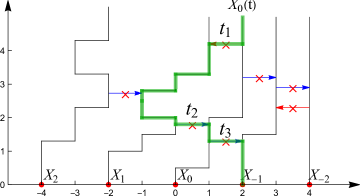
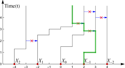
Backwards geodesic and index process in the TASEP setting were introduced in [26], see also [30]. For TASEP they have many properties similar to geodesics in the last passage percolation models. Physically they track the space-time locations where the randomness is relevant for the position of the particles at time $t$. We extend its definition also to generic SEP, which includes ASEP and ASEPsc, and numerically investigate some (conjecturally universal) statistics.

Definition 2.1 (Backwards geodesic and index process).

For any fixed $N\in\mathbb{Z}$ and $t\geq 0$, we call $(N(t\downarrow s))_{s\in[0,t]}$ as the backwards index process of particle $N$ starting from time $t$ and running backwards in time. It is defined as follows111In the notation, we do not explicitly write the dependence on $N$.:

  1. 1.

    At time $t$, we set $N(t\downarrow t)=N$.

  2. 2.

    The label changes at time $s\in[0,t)$ if the following occur:

    1. (a)

      there exists a suppressed right to left jump of particle $X_{N(t\downarrow s^{+})}$, then we set $N(t\downarrow s)=N(t\downarrow s^{+})-1$,

    2. (b)

      there exists a suppressed left to right jump of particle $X_{N(t\downarrow s^{+})}$, then we set $N(t\downarrow s)=N(t\downarrow s^{+})+1$.

The trajectory $(X_{N(t\downarrow s)})_{s\in[0,t]}$ is called the backwards geodesic of particle $N$ starting from time $t$. $N(t\downarrow 0)$ is called the end-point of the backwards geodesic.

Refer to caption
Figure 3: Illustration for backwards geodesic in ASEP setting for the index $N=0$. From left to right, the black solid lines are the space-time trajectory of particles $X_{2}$, $X_{1}$, $X_{0},\ X_{-1}$ and $X_{-2}$ respectively. The arrow with a cross stands for a suppressed jump. The green line is the trajectory of backwards geodesic of particle $X_{0}$. $t_{1},t_{2}$ and $t_{3}$ are the times when $N(t\downarrow s)$ changes its value, for instance, at time $t_{2}$, since particle $X_{1}$ has a right suppressed jump, we set $N(t\downarrow t_{2})=N(t\downarrow t_{2}^{+})-1$.
Construction of ASEP.

To state the properties of backwards index process, we recall the following construction of ASEP [28], on which Poisson clocks are assigned to particle labels. We have a family of independent Poisson processes $\{T_{m}^{+},T_{m}^{-}\}_{m\in\mathbb{Z}}$ where $T_{m}^{+}$ has parameter $p$ and $T_{m}^{-}$ has parameter $1-p$. The points of the Poisson process $T_{m}^{+}$ (resp. $T_{m}^{-}$) are the time when a particle with label $m$ attempts to jump to its right (resp. left), and the jump is successful provided the arrival site is empty. By the independence of the Poisson processes, almost surely, there are no simultaneous jump trials. Moreover, for each fixed $t\geq 0$, almost surely there exist infinitely many positive and negative integers $m$ such that there exist no Poisson points of $T_{m}^{+}$ and $T_{m}^{-}$ in the time interval $[0,t]$ so that the construction is well-defined (in the same way Harris graphical construction for the basic coupling is well-defined [37, 36, 41]).

We couple two processes $X(t)$ and $Y(t)$ with different initial conditions $X(0)$ and $Y(0)$ such that particle $X_{i}$ and $Y_{i}$ use the same clocks $(T_{i}^{+},T_{i}^{-})$ for all $i\in\mathbb{Z}$. This is called the clock coupling [28]. For two configurations $X,\ Y$, we define a partial order $X\preceq Y$ if $X(i)\leq Y(i)$ for all $i\in\mathbb{Z}$. As for the basic coupling, the clock coupling also preserves the partial ordering.

Lemma 2.2 (Lemma 3.9 of [28]).

Under clock coupling, if $X(0)\preceq Y(0)$, then we have $X(s)\preceq Y(s)$ for all $s\geq 0$ almost surely.

Next, we define a process, with step initial condition, coupled with $X$, in such a way that particle $n-M$ uses the same clocks as particle $n$ of the process $X$. To keep track of the coupling with $X$ and the shift of the clocks by $M$, we will call the new process $X^{\mathrm{step},X,M}$.

Definition 2.3.

Let $X(t)$ be ASEP and $M\in\mathbb{Z}$ be fixed. We define the process $X^{{\rm step},X,M}(t)$ as follows:

  1. 1.

    Initial condition:

    $$X^{\mathrm{step},X,M}_{n}(0)=\begin{cases}-n,\quad&\mathrm{if}\ n\geq 0,\\ \infty,&\mathrm{otherwise}.\end{cases}$$ (2.8)
  2. 2.

    Time evolution: for each $i\in\mathbb{Z}$, we let $X^{\mathrm{step},X,M}_{i-M}(t)$ and $X_{i}(t)$ use the same Poisson processes $(T_{i}^{+},T_{i}^{-})$.

For TASEP, it was shown in [26, 52] that

$$X_{N}(t)=\min_{M\leq N}\left\{X_{N-M}^{\mathrm{step},X,M}(t)+X_{M}(0)\right\}=X_{N-N(t\downarrow 0)}^{\mathrm{step},{X,{N(t\downarrow 0)}}}(t)+X_{N(t\downarrow 0)}(0)$$ (2.9)

almost surely for all $N\in\mathbb{Z}$ and $t\geq 0$.

Remark 2.4.

TASEP was known to satisfy the skew-time reversibility [42], which states:

$\displaystyle\mathbb{P}\left(X_{n}(t)\geq s\right)=\mathbb{P}\left(\hat{X}_{n}(t)\leq X_{n}(0),\hat{X}_{n-1}(t)\leq X_{n-1}(0),\ldots,\hat{X}_{n-m}(t)\leq X_{n-m}(0)\right),$ (2.10)

where $\hat{X}(t)$ is TASEP with left drift (i.e., $q=1$ and $p=0$) and initial condition

$$\hat{X}_{r}(0)=\begin{cases}s+(n-r),\quad&\text{if}\ r\leq n,\\ -\infty,&\text{otherwise}.\end{cases}$$ (2.11)

Note that the initial condition $\hat{X}(t)$ is a step initial condition. Hence, skew-time reversibility establishes a connection between general initial condition and step initial condition. Backwards geodesic provides the same property.

For ASEP with $p<1$, these equalities are not anymore true, but

$$X_{N-N(t\downarrow 0)}^{\mathrm{step},{X,{N(t\downarrow 0)}}}(t)+X_{N(t\downarrow 0)}(0)\geq\min_{M\leq N}\left\{X_{N-M}^{\mathrm{step},X,M}(t)+X_{M}(0)\right\}\geq X_{N}(t).$$ (2.12)
Lemma 2.5.

Let $X(t)$ be ASEP with jump rate (2.4), then, almost surely,

$$D_{N}(t)=X_{N-N(t\downarrow 0)}^{\mathrm{step},{X,{N(t\downarrow 0)}}}(t)+X_{N(t\downarrow 0)}(0)-X_{N}(t)\geq 0.$$ (2.13)
Proof.

Let $Y(t)$ be a ASEP with initial condition

$$Y_{n}(0)=\begin{cases}X_{n}(0),\quad&\mathrm{if}\ n\geq N(t\downarrow 0),\\ \infty,&\mathrm{otherwise},\end{cases}$$ (2.14)

and couple $Y(t)$ and $X(t)$ via clock coupling. By Lemma 2.2, we have almost surely $X(t)\preceq Y(t)$. Define process $Z(t)$ as

$$Z_{m}(t)=X_{m-N(t\downarrow 0)}^{\mathrm{step},{X,{N(t\downarrow 0)}}}(t)+X_{N(t\downarrow 0)}(0).$$ (2.15)

Then by Definition 2.3, we have

Zm(0)=(2.8)mYm(0),mN(t0),Z_{m}(0)\stackrel{{\scriptstyle\eqref{ini}}}{{=}}-m\geq Y_{m}(0),\quad\forall m\geq N(t\downarrow 0), (2.16)

and particle $Z_{m}$ and $Y_{m}$ use the same Poisson clock. Using Lemma 2.2 once again, we obtain

$$Z_{m}(t)\geq Y_{m}(t)\geq X_{m}(t),\quad\forall m\geq N(t\downarrow 0),\ t\geq 0,$$ (2.17)

from which (2.13) follows. ∎

2.3 Observables

2.3.1 Limit behaviour of the end-point of the backwards geodesic

In this paper, we consider flat non-random initial condition with density $1/2$, that is

$$X_{n}(0)=-2n,\quad\forall n\in\mathbb{Z}.$$ (2.18)

The first observable we are interested in is the end-point of the backwards geodesic, that is, $X_{N(t\downarrow 0)}(0)$.

In TASEP, backwards geodesic could be viewed as analog of geodesics in the last passage percolation models [15]. Therefore the law of $X_{N(t\downarrow 0)}(0)$ should converges in the scaling limit to the end-point of the geodesics for last passage percolation for the point-to-line problem. This is given by

$$\hat{u}=\operatorname*{argmax}_{u\in\mathbb{R}}\{{\cal A}_{2}(u)-u^{2}\},$$ (2.19)

where ${\cal A}_{2}$ is Airy2 process [47].

In [39] it is proven that222To be precise, it is proven under the assumption of uniqueness of $\hat{u}$, which was subsequently shown in [21]. $\lim_{N\to\infty}\mathcal{T}_{N}\stackrel{{\scriptstyle d}}{{=}}\hat{u}$, where $\mathcal{T}_{N}$ is the endpoint of geodesic in a point-to-point last passage percolation (LPP) setting. We show a similar result for the end-point of the backwards geodesic in TASEP.

Theorem 2.6.

Consider TASEP with flat initial condition (2.18). Then, for any $N\in\mathbb{Z}$, we have $\lim_{t\to\infty}B^{\rm TASEP}_{t}\stackrel{{\scriptstyle d}}{{=}}\hat{u}$, where

$$B^{\rm TASEP}_{t}=\frac{X_{N(t\downarrow 0)}(0)-X_{N}(0)-t/2}{2^{1/3}t^{2/3}}.$$ (2.20)

Based on KPZ scaling theory [54], which will be discussed in more detail in Section 3.2, we get the following predictions for ASEP and ASEPsc.

Conjecture 2.7.

Consider ASEP with flat initial condition (2.18). Then for any $N\in\mathbb{Z}$ we have $\lim_{t\to\infty}B^{\rm ASEP}_{t}\stackrel{{\scriptstyle d}}{{=}}\hat{u}$, where

$$B^{\rm ASEP}_{t}=\frac{X_{N(t\downarrow 0)}(0)-X_{N}(0)-(p-q)t/2}{2^{1/3}((p-q)t)^{2/3}}.$$ (2.21)

To state the conjecture for ASEPsc, we need additional assumptions on its jump rate, under which the invariant measure is known [40] and it allows us to compute analytically all model-dependent parameters in the scaling conjecture. Fix parameters $\beta,E\in\mathbb{R}$ and choose the jump rates in (2.5), (2.6) as

$$\begin{array}[]{lll}\alpha_{2}=1,&\alpha_{3}=\frac{1}{2}\left(1+e^{-\beta}\right),&\alpha_{4}=e^{-\beta},\\[10.00002pt] \gamma_{2}=e^{-\beta}e^{-E},&\gamma_{3}=\frac{1}{2}\left(1+e^{-\beta}\right)e^{-E},&\gamma_{4}=e^{-E}.\end{array}$$ (2.22)
Conjecture 2.8.

Consider ASEPsc, with flat initial condition (2.18) and rates given by (2.22). Then, for any $N\in\mathbb{Z}$, we have $\lim_{t\to\infty}B^{{\rm ASEPsc}}_{t}\stackrel{{\scriptstyle d}}{{=}}\hat{u}$, where

$$B^{{\rm ASEPsc}}_{t}=\frac{X_{N(t\downarrow 0)}(0)-X_{N}(0)-2J(\beta,E)t}{2^{1/3}t^{2/3}\Gamma(\beta,E)^{2/3}A(\beta)^{-1}},$$ (2.23)

where

$\displaystyle J(\beta,E)$ $\displaystyle=\frac{1-e^{-E}}{2\left(e^{\beta/2}+e^{\beta}\right)},\quad A(\beta)=\frac{e^{\beta/2}}{4},$ (2.24)
$\displaystyle\Gamma(\beta,E)$ $\displaystyle=\frac{\left(3e^{\beta/2}-1\right)\left(1-e^{-E}\right)}{e^{\beta/2}+e^{\beta}}.$

In Section 4.1.1 we present the numerical simulations confirming Conjecture 2.7 and in Section 4.2.2 for Conjecture 2.8.

2.3.2 Particle’s position in speed changed ASEP

The KPZ scaling theory explained in Section 3.2 leads also to the following conjecture for the limiting distribution of particle’s position in ASEPsc.

Conjecture 2.9.

For ASEPsc with initial condition (2.18). Define the rescaled process

$$X^{\rm resc}_{N}(t)=\frac{X_{N}^{{\textrm{ASEPsc}}}(t)-X^{\textrm{ASEPsc}}_{N}(0)-2J(\beta,E)t}{-2\Gamma(\beta,E)^{1/3}t^{1/3}}.$$ (2.25)

Then, for any $N\in\mathbb{Z}$, we have

$$\lim_{t\to\infty}\mathbb{P}\left(X^{\rm resc}_{N}(t)\leq s\right)=F_{\rm GOE}(2s),\quad\forall s\in\mathbb{R},$$ (2.26)

where $F_{{\rm GOE}}$ is Tracy-Widom GOE distribution [57].

In Section 4.2.1 we numerically show that this conjecture holds true.

2.3.3 Discrepancy for ASEP

Recall that $D_{N}(t)$ defined in (2.13) is generally not zero in ASEP, but positive. Moreover, $D_{N}(t)$ is an upper bound for the discrepancy between $\min_{M\leq N}\{X_{N-M}^{\mathrm{step},X,M}(t)+X_{M}(0)\}$ and $X_{N}(t)$. From recent results on ASEP, it follows that

Lemma 2.10.

We have

$$\lim_{t\to\infty}\frac{\min_{M\leq N}\{X_{N-M}^{\mathrm{step},X,M}(t)+X_{M}(0)\}-X_{N}(t)}{t^{1/3}}=0$$ (2.27)

in probability.

Proof.

It is enough to show $\lim_{t\to\infty}D^{{\rm resc}}_{N}(t)\stackrel{{\scriptstyle d}}{{=}}0$, where

$$D^{{\rm resc}}_{N}(t):=\frac{\min_{M\leq N}\{X_{N-M}^{\mathrm{step},X,M}(t)+X_{M}(0)\}}{t^{1/3}}-\frac{X_{N}(t)}{t^{1/3}}.$$ (2.28)

Recall that $X(t)$ is ASEP with flat initial condition with asymmetric parameter $p$. For $t>0,$ we define $\hat{t}:=(2p-1)t.$ Without loss of generality, we set $N=\hat{t}/4$. We have, see [43, 48],

$$\lim_{t\to\infty}\mathbb{P}\left(\frac{X_{N}(t)}{-\hat{t}^{1/3}}\leq s\right)=F_{{\rm GOE}}(2s).$$ (2.29)

By (2.13), we have

$\displaystyle\frac{X_{N}(t)}{-\hat{t}^{1/3}}$ $\displaystyle\leq\max_{M\leq N}\frac{X_{N-M}^{{\rm step},X,M}+X_{M}(0)}{-\hat{t}^{1/3}}$ (2.30)
$\displaystyle\leq 2^{-1/3}\max_{u\geq 2^{-4/3}\hat{t}^{1/3}}\frac{X_{\hat{t}/4+2^{-2/3}\hat{t}^{2/3}u}^{{\rm step},X,-2^{-2/3}\hat{t}^{2/3}u}(t)+2^{1/3}\hat{t}^{2/3}u}{-2^{-1/3}\hat{t}^{1/3}},$

where in the second step we parameterize $M$ by $-2^{-2/3}\hat{t}^{2/3}u$.

In [48], it is showed that in the $t\to\infty$ limit the r.h.s. of (2.30) converges to $2^{-1/3}T$ with $T=\max_{u\in\mathbb{R}}\left\{A_{2}(u)-u^{2}\right\}$. It is known that $\mathbb{P}\left(2^{-1/3}T\leq s\right)=F_{{\rm GOE}}(2s)$ [39].

This means that, properly rescaled, both terms in the r.h.s. of (2.28) converge to the same distribution as $t\to\infty$, and since $D^{{\rm resc}}_{N}(t)\geq 0$ one stochastically dominated the other. This implies that $D^{{\rm resc}}_{N}(t)$ scaled by $t^{-1/3}$ converges to 0, see for instance Lemma 4.1 of [13]. ∎

If $N(t\downarrow 0)$ is close to the minimization index, then we would also expect that $D_{N}(t)/t^{1/3}\to 0$ as $t\to\infty$. However, it remains unclear whether the unscaled discrepancy $D_{N}(t)$ diverge or converge to a non-degenerate random variable as $t\to\infty$. Our numerical simulation indicates that the latter is the case.

Conjecture 2.11.

There exists a non-degenerate (discrete) distribution $G$ such that

$$\lim_{t\to\infty}\mathbb{P}\left(D_{N}(t)\leq s\right)=G(s),\quad\forall s\in\mathbb{R}.$$ (2.31)

In Section 4.1.2 we provide numerical evidence of Conjecture 2.11.

3 Analytic results

In this section we will show Theorem 2.6 and calculate the explicit formula mentioned in several conjectures above.

3.1 Proof of Theorem 2.6

In the whole section, we will assume $X(t)$ is a TASEP with $X_{n}(0)=-2n$ for all $n\in\mathbb{Z}$. For a fixed $N$, recall that $N(t\downarrow 0)$ is the end-point of the backwards geodesic of particle $X_{N}$ starting from time $t$ (see Definition 2.1). Define

$$\hat{u}=\operatorname*{argmax}_{u\in\mathbb{R}}\{{\cal A}_{2}(u)-u^{2}\},$$ (3.1)

where ${\cal A}_{2}$ is the $\mathrm{Airy}_{2}$ process. Since $X_{n}(0)=-2n$ for all $n\in\mathbb{Z}$, the statement of Theorem 2.6 is equivalent to $\lim_{t\to\infty}u_{t}\stackrel{{\scriptstyle d}}{{=}}\hat{u}$, where

$$u_{t}=\frac{N-N(t\downarrow 0)-t/4}{2^{-2/3}t^{2/3}}.$$ (3.2)

The strategy is as follows. Let $X^{{\rm step}}(t)$ be TASEP with step initial condition, i.e., $X_{n}(0)=-n$ for all $n\geq 0$ and define the rescaled process

$$H_{t}(x)=\frac{X^{\mathrm{step}}_{\lfloor t/4+2^{-2/3}t^{2/3}x\rfloor}(t)+2^{1/3}t^{2/3}x}{-2^{-1/3}t^{1/3}},\quad\forall x\geq-2^{-4/3}t^{1/3}$$ (3.3)

and

$$\hat{u}_{t}=\inf\big{\{}x\geq-2^{-4/3}t^{1/3}\big{|}H_{t}(x)=\max_{y}H_{t}(y)\big{\}}.$$ (3.4)

In Lemma 3.2, we will show that, for any fixed $t>0$,

$$u_{t}\stackrel{{\scriptstyle d}}{{=}}\hat{u}_{t}.$$ (3.5)

It is then enough to show $\hat{u}_{t}\to\hat{u}$ in distribution as $t\to\infty$. By Proposition 2.9 in [15], $H_{t}(u)\to{\cal A}_{2}(u)-u^{2}$ weakly on $C([-L,L])$ for any $0<L<\infty$. Together with the tightness of the distribution of $\hat{u}_{t}$ (see Lemma 3.3 below) and the uniqueness of $\operatorname*{argmax}_{u\in\mathbb{R}}\{{\cal A}_{2}(u)-u^{2}\}$ (see for instance [21, Theorem 4.3], [35],[44]), we conclude that $\hat{u}_{t}$ converges in distribution to $\hat{u}$ (see Proposition 3.5 below). Together with (3.5), we then obtain Theorem 2.6.

3.1.1 Proof of the identity (3.5)

The starting point is the following observation.

Lemma 3.1.

Let $X(t)$ be an arbitrary TASEP with initial condition $X(0)$, and $X^{\mathrm{step},X,M}$ be defined as in Definition 2.3. Then, for any $t\geq 0$ and $N\in\mathbb{Z}$, we have

$$N(t\downarrow 0)=\max\{n\leq N|X^{\mathrm{step},X,n}_{N-n}(t)+X_{n}(0)=X_{N}(t)\}$$ (3.6)

see Figure 4 for an illustration.

Refer to caption
Refer to caption
Figure 4: Illustration for Lemma 3.1. On the left panel: from left to right, the black solid lines represent the trajectory of particles $X_{2},\ X_{1},\ X_{0},\ X_{-1}$, and $X_{-2}$ respectively. The green line is the backwards trajectory of particle $X_{1}$ from time $t$. The end-point of this trajectory is $X_{-1}$. Note that $X_{1}(t=5)=1$. On the right panel: from right to left, the black solid lines represent the trajectories of particles $X_{0}^{{\rm step},X,0}$, $X_{1}^{{\rm step},X,0}$, and so on. In particular, note that $0>-1=N(t\downarrow 0)$ and $X_{1}^{{\rm step},X,0}(t=5)=2>1=X_{1}(t=5)$.
Proof.

By (2.9), $N(t\downarrow 0)\in\{n\leq N|X^{{\rm step},X,n}_{N-n}(t)+X_{n}(0)=X_{N}(t)\}$. Let $M\in(N(t\downarrow 0),N]$ and we show that

$$X_{m-M}^{{\rm step},X,M}(t)+X_{M}(0)\geq X_{m}(t)+1,\quad\forall m\in[M,N].$$ (3.7)

We define a new process $Z(t)$ with initial condition

$$Z_{n}(0)=\begin{cases}X_{n}(0),\quad&{\rm if}\ n\geq M,\\ \infty,&{\rm otherwise}\end{cases}$$ (3.8)

with $Z_{n}$ sharing the same Poisson clocks with $X_{n}$. By monotonicity property (see Lemma 2.2), we have $X_{m-M}^{{\rm step},X,M}(t)+X_{M}(0)\geq Z_{m}(t)$. By definition of backwards geodesic, for each $m\in[M,N]$, there exists

$$t_{N}>t_{N-1}>\cdots>t_{M}$$ (3.9)

such that at time $t_{m}$ particle $X_{m}$ has a right suppressed jump by the presence of $X_{m-1}$. We claim that

$$Z_{m}(s)\geq X_{m}(s)+1,\quad\forall m\in[M,N],\ s\in(t_{m},t].$$ (3.10)

We show this via induction on $m$. For $m=M$, since $Z_{M-1}(s)=\infty$ for all $s\geq 0$, the attempted jump at $t_{M}$ will be a successful one for $Z_{M}$, hence, we have $Z_{M}(t_{M}^{+})\geq X_{M}(t_{M}^{+})+1$. This also implies $Z_{M}(s)\geq X_{M}(s)+1$ for all $s>t_{M},$ since $Z_{M}$ and $X_{M}$ shares the same Poisson clock. Suppose now $Z_{N-1}(s)\geq X_{N}(s)+1$ for all $s>t_{N-1}$, then $Z_{N-1}(t_{N})\geq X_{N-1}(t_{N})+1$, thus, the attempted jump at $t_{N}$ will also be successful for $Z_{N}$ and hence $Z_{N}(t_{N}^{+})\geq X_{N}(t_{N}^{+})+1$. Using monotonicity property once more, we then obtain $Z_{N}(t)\geq X_{N}(t)+1$. ∎

Applying (2.9), $X_{n}(0)=-2n$ for all $n\in\mathbb{Z}$ and Lemma 3.1, we obtain

$$N(t\downarrow 0)=\max\left\{n\leq N\,\Big{|}\,X^{{\rm step},X,n}_{N-n}(t)-2n=\min_{m\leq N}\left\{X^{{\rm step},X,m}_{N-m}(t)-2m\right\}\right\}.$$ (3.11)
Lemma 3.2.

For fixed $t\geq 0$, it holds $u_{t}\stackrel{{\scriptstyle d}}{{=}}\hat{u}_{t}$.

Proof.

Choose a fixed $t\geq 0$. By the spatial homogeneity, we only need to show the case for $N=\tfrac{t}{4}$. Define now $n(x)=2^{-2/3}t^{2/3}x$, $Z_{m}^{n}=X^{{\rm step},X,n}_{m}(t)$, and

$$W(t)=\min_{x\geq-2^{-4/3}t^{1/3}}\left\{Z^{{n(x)}}_{t/4+n(x)}(t)+2n(x)\right\}.$$ (3.12)

Then by (3.11), we have

$\displaystyle N(t\downarrow 0)=\max\left\{n\leq t/4\,\Big{|}\,Z^{n}_{t/4-n}(t)-2n=\min_{m\leq t/4}\left\{Z^{m}_{t/4-m}(t)-2m\right\}\right\}$ (3.13)
$\displaystyle=$ $\displaystyle-2^{-2/3}t^{2/3}\min\left\{x\geq-2^{-4/3}t^{1/3}\,\Big{|}\,Z^{{n(x)}}_{t/4+n(x)}(t)+2n(x)=W(t)\right\}$
$\displaystyle\stackrel{{\scriptstyle d}}{{=}}$ $\displaystyle-2^{-2/3}t^{2/3}\inf\left\{x\geq-2^{-4/3}t^{1/3}|H_{t}(x)=\max H_{t}(y)\right\}=-2^{-2/3}t^{2/3}\hat{u}_{t},$

where in the second last step we use the fact that $X^{{\rm step}}$ and $X^{{\rm step},X,M}$ have the same distribution for all $M\leq N$. ∎

3.1.2 Localization

Finally we need to show $\lim_{t\to\infty}\hat{u}_{t}\stackrel{{\scriptstyle d}}{{=}}\hat{u}$. First, we establish the following tightness result for $\hat{u}_{t}$:

Lemma 3.3.

For any $L>0$, there exists $T=T(L)>0$ such that

$$\mathbb{P}\left(|\hat{u}_{t}|>L\right)\leq Ce^{-cL}\quad\forall t\geq T(L)$$ (3.14)

for constants $C,c>0$ independent on $L$.

Remark 3.4.

A similar result was previously obtained in the context of LPP; see (4.21) of [32]. However, additional steps are required to translate this result into the setting of TASEP. Therefore, we provide a direct proof here, without relying on the connection to LPP.

The proof is postponed to the end of this section. Lemma 3.3 direcly implies

Proposition 3.5.

Let $\hat{u}_{t}$ be defined as (3.4), then

$$\lim_{t\to\infty}\hat{u}_{t}\stackrel{{\scriptstyle d}}{{=}}\hat{u}.$$ (3.15)
Proof.

We define the functional $\operatorname*{sargmax}$ [39] on $C([-L,L])$ (without dependence on $L$ for notation) as:

$$\operatorname*{sargmax}_{|x|\leq L}f(x)=\inf\Big{\{}u\geq-L\,\big{|}\,\max_{x\in[-L,u]}f(x)=\max_{x\in[-L,L]}f(x)\Big{\}}.$$ (3.16)

Additionally,

$$\hat{u}_{t}^{L}=\operatorname*{sargmax}_{|x|\leq L}H_{t}(x),\quad\textrm{and}\quad\hat{u}^{L}=\operatorname*{sargmax}_{|x|\leq L}\left({\cal A}_{2}(u)-u^{2}\right).$$ (3.17)

By the triangle inequality we obtain

$\displaystyle\left|\mathbb{P}\left(u_{t}\leq x\right)-\mathbb{P}(\hat{u}\leq x)\right|$ (3.18)
$\displaystyle\leq$ $\displaystyle\left|\mathbb{P}\left(u_{t}^{L}\leq x\right)-\mathbb{P}\left(\hat{u}^{L}\leq x\right)\right|+\mathbb{P}\left(\hat{u}^{L}\neq\hat{u}\right)+\mathbb{P}\left(u_{t}\neq u_{t}^{L}\right).$

Since the maximizer of $\mathcal{A}_{2}(u)-u^{2}$ is unique, it is a continuous point of the functional $\operatorname*{sargmax}$. Thus, by weak convergence, the first term in the right-hand side of (3.18) converges to 0 as $t\to\infty$. Moreover, [39] shows that $\mathbb{P}\left(\hat{u}\neq\hat{u}^{L}\right)\leq\epsilon$ for large $L$. By Lemma 3.3, the third probability is also arbitrarily small for sufficiently large $L$. Thus taking first $t\to\infty$ and then $L\to\infty$ we get that |(3.18)|2ε|\eqref{triangle}|\leq 2\varepsilon for any $\varepsilon>0$, which concludes the proof. ∎

We adapt the method for Proposition 1.4 in [39] to prove Lemma 3.3. Recall $H_{t}(u)$ defined in333We drop the ’step’ in the notation in below. (3.3). We define

$$S_{t}^{\infty}=\max_{u\geq 2^{-4/3}t^{1/3}}H_{t}(u),\quad S_{t}^{L}=\max_{u\in[-L,L]}H_{t}(u).$$ (3.19)
Lemma 3.6.

For any $L>0$, there exists $T=T(L)>0$ such that

$$\mathbb{P}\left(S_{t}^{\infty}\neq S_{t}^{L}\right)\leq Ce^{-cL}\quad\forall t\geq T(L).$$ (3.20)
Proof.

Choose $\varepsilon>0$. For arbitrary $A\in\mathbb{R}$, we have

$$\left\{H_{t}(0)>A\right\}\cap\Big{\{}\max_{u\not\in[-L,L]}H_{t}(u)<A\Big{\}}\subset\{S_{t}^{\infty}=S_{t}^{L}\}.$$ (3.21)

Thus,

$$\mathbb{P}\left(S_{t}^{\infty}\neq S_{t}^{L}\right)\leq\mathbb{P}\left(H_{t}(0)\leq A\right)+\mathbb{P}\left(\max_{u\not\in[-L,L]}H_{t}(u)\geq A\right).$$ (3.22)

Choosing $A=-2^{-3}L^{2}$, we have444Combining Proposition B.1 and (56) in [2], one obtains the upper bound for LPP in point-to-point setting, i.e., $\mathbb{P}\left(L_{\ell}^{\mathrm{resc}}\leq s\right)\leq Ce^{-c|s|^{3/2}},$ where $L_{\ell}^{\mathrm{resc}}$ is the rescaled last passage time from $(0,0)$ to $(\ell,\ell)$. Using the fact that the maximal last passage time from line $\mathcal{L}=\{(k,-k),k\in\mathbb{Z}\}$ to $(\ell,\ell)$ is larger than the one from $(0,0)$ to $(\ell,\ell)$, one also obtain the upper bound for LPP in point-to-line setting, see also Proposition B.1 (c) in [34].

$$\mathbb{P}\left(H_{t}(0)\leq A\right)=\mathbb{P}\left(X_{t/4}\geq 2^{-3}L^{2}t^{1/3}\right)\leq Ce^{-cL^{3}}.$$ (3.23)

We can bound the second term on the right hand side of (3.22) as

$$\mathbb{P}\left(\max_{u\not\in[-L,L]}H_{t}(u)\geq A\right)\leq\underbrace{\mathbb{P}\left(\max_{u\geq L}H_{t}(u)\geq A\right)}_{=:\operatorname{I}}+\underbrace{\mathbb{P}\left(\max_{u\in[2^{-4/3}t^{1/3},-L]}H_{t}(u)\geq A\right)}_{=:\operatorname{II}}.$$ (3.24)

It remains to control the two terms on the right hand side. Using definition of $H_{t}(x)$, we have

$\displaystyle\operatorname{I}=\mathbb{P}\left(\min_{n\leq-2^{-2/3}t^{2/3}L}\{X_{t/4-n}(t)-2n\}\leq 2^{-10/3}t^{1/3}L^{2}\right)$ (3.25)
$\displaystyle=$ $\displaystyle\mathbb{P}\bigg{(}\min_{n\in[-\frac{t}{4}-L^{2}t^{1/3},-2^{-2/3}t^{2/3}L]}\{X_{t/4-n}(t)-2n\}\leq 2^{-10/3}t^{1/3}L^{2}\bigg{)}$
$\displaystyle\leq$ $\displaystyle\mathbb{P}\bigg{(}\min_{n\in[-\frac{t}{4}-L^{2}t^{1/3},-\frac{t}{4}]}\{X_{t/4-n}(t)-2n\}\leq 2^{-10/3}t^{1/3}L^{2}\bigg{)}$
$\displaystyle+$ $\displaystyle\mathbb{P}\bigg{(}\min_{n\in[-\frac{t}{4},-2^{-2/3}t^{2/3}L]}\{X_{t/4-n}(t)-2n\}\leq 2^{-10/3}t^{1/3}L^{2}\bigg{)},$

where the second equality follows from

$\displaystyle X_{t/4-n}(t)-2n\geq-n-\frac{t}{4}\geq L^{2}t^{1/3}$ (3.26)

for all $n\leq-\frac{t}{4}-L^{2}t^{1/3}$ and $t\geq 0$, since $X(t)$ is TASEP with step initial condition. Setting $\gamma=\frac{1}{4}$, $T=2t$ and $K=2^{-7/3}L$ in (4.53) of [28], one obtains that the probability on the last line of (3.25) is smaller than $Ce^{-cL}$. Note that

$$2^{-10/3}L^{2}t^{1/3}-2n\leq(1-2\sqrt{1/4+nt^{-1}})t-(n^{2}t^{-4/3}-\alpha^{2})t^{1/3}$$ (3.27)

for all $n\in[Lt^{2/3},t/4+L^{2}t^{1/3}].$ The term on the second last line of (3.25) is bounded by

$\displaystyle\sum_{n=t/4}^{t/4+L^{2}t^{1/3}}\mathbb{P}\left(X_{t/4+n}(t)\leq(1-2\sqrt{1/4+nt^{-1}})t-(n^{2}t^{-4/3}-L^{2})t^{1/3}\right)$ (3.28)
$\displaystyle\leq$ $\displaystyle CL^{2}t^{1/3}e^{-c(t^{2/3}/16-L^{2})}\leq Ce^{-cL^{2}}$

for all $t\geq(8L)^{3}$. Thus $\operatorname{I}\leq Ce^{-cL}$ for some constants $C,c>0$. It remains to control $\operatorname{II}.$ Applying definition of $H_{t}(x)$, we have

$\displaystyle\operatorname{II}=\mathbb{P}\left(\min_{u\in[2^{-2/3}Lt^{2/3},\frac{t}{4}]}\left\{X_{t/4-n}(t)-2n\right\}\leq L^{2}t^{1/3}\right).$ (3.29)

Let $X^{{\rm hf}}(t)$ be TASEP with half flat initial condition, i.e.,

$$X^{{\rm hf}}_{n}(0)=\begin{cases}-2n,\quad&\mathrm{if}\ n\geq 0,\\ \infty,&\mathrm{otherwise}.\end{cases}$$ (3.30)

By (2.9), we have

$\displaystyle X^{{\rm hf}}_{t/4-2^{-2/3}Lt^{2/3}}(t)=\min_{M\in[0,t/4-2^{-2/3}Lt^{2/3}]}\left\{X^{{\rm step},X^{{\rm hf}},M}_{t/4-2^{-2/3}Lt^{2/3}-M}(t)-2M\right\}$ (3.31)
$\displaystyle=$ $\displaystyle\min_{n\in[2^{-2/3}Lt^{2/3},\frac{t}{4}]}\left\{X^{{\rm step},X^{{\rm hf}},M}_{t/4-n}(t)-2n\right\}-2^{1/3}Lt^{2/3}.$

In other words, there exists a coupling between $X(t)$ and $X^{{\rm hf}}(t)$ such that

$$\min_{n\in[2^{-2/3}Lt^{2/3},\frac{t}{4}]}\left\{X_{t/4-n}(t)-2n\right\}=X^{{\rm hf}}_{t/4-2^{-2/3}Lt^{2/3}}(t)-2^{1/3}Lt^{2/3}.$$ (3.32)

Then we have555This comes from the proof of Theorem 2.6 in [20]. To see this, we set $\ell=t$, $s=0$ and $kM=2^{2/3}\alpha$, then (2.33) in [20] will become (3.33) in our setting.

$$\operatorname{II}=\mathbb{P}\left(X^{{\rm hf}}_{t/4-2^{-2/3}Lt^{2/3}}(t)-2^{1/3}Lt^{2/3}\leq L^{2}t^{1/3}\right)\leq Ce^{-cL}.$$ (3.33)

This finishes the proof.

Proof of Lemma 3.3.

Note that $\{\hat{u}_{t}>L\}\subset\{S_{t}^{L}\neq S_{t}^{\infty}\}$, hence we have

$$\mathbb{P}\left(\hat{u}_{t}>L\right)\leq Ce^{-cL}$$ (3.34)

for $t$ large. Also, we have $\{\hat{u}_{t}<-L\}\subset\{\max_{u\in[2^{-4/3}t^{1/3},-L]}H_{t}(u)\geq A\}\cup\{H_{t}(0)\leq A\}$ for arbitrary $A$. Choosing $A$ as the one in proof of the previous lemma, we have

$$\mathbb{P}\left(\hat{u}_{t}<-L\right)\leq Ce^{-cL}$$ (3.35)

by (3.23) and (3.33). ∎

3.2 KPZ scaling theory

The KPZ scaling theory [54], see also further details in Section 6 of [46], provides a universal scaling formula for models in the KPZ class. After presenting the formulas conjectures by the KPZ sclaing theory, we compute the universal constants using results from TASEP. The model-dependent quantities are easy to compute for ASEP, but more involved for ASEPsc.

Let $\eta_{t}$ be a general exclusion process with generator (2.2).

Assumption 3.7 ([54]).

The spatially ergodic and time stationary measures of the process $\eta_{t}$ are precisely labeled by the average density

$$\rho=\lim_{a\rightarrow\infty}\frac{1}{2a+1}\sum_{|j|\leq a}\eta(j)$$ (3.36)

with $|\rho|\leq 1$.

Denote $\mu_{\rho}$ as the stationary measure satisfying Assumption 3.7. Define the stationary current as

$\displaystyle J(\rho)=$ $\displaystyle\mu_{\rho}\left(c_{\eta}(0,1)\eta(0)(1-\eta(1))\right)-\mu_{\rho}\left(c_{\eta}(1,0)\eta(1)(1-\eta(0))\right)$ (3.37)

and integrated stationary covariance as

$$A(\rho)=\sum_{j\in\mathbb{Z}}(\mu_{\rho}\left(\eta(0)\eta(j)\right)-\mu_{\rho}\left(\eta(0)\right)^{2})=\sum_{j\in\mathbb{Z}}(\mu_{\rho}\left(\eta(0)\eta(j)\right)-\rho^{2}).$$ (3.38)

Set $\Gamma(\rho)=-A(\rho)^{2}J^{\prime\prime}(\rho)$.

3.2.1 Scaling for particle’s position

As explained in [46], the fluctuations of the integrated current (height function) in KPZ models should be scaled by $\Gamma(\rho)^{1/3}t^{1/3}$ and the spatial scaling around the macroscopic behaviour should be scaled by $\Gamma(\rho)^{2/3}A(\rho)^{-1}t^{2/3}$. The height function is defined by setting $h(0,0)=0$, $h(0,t)=2J(t)$, with $J(t)$ then integrated particle current at 0 in the time interval $[0,t]$ and $h(x+1,t)-h(x,t)=1-2\eta_{t}(x)$.

For initial condition $x_{n}(0)=-\lfloor n/\rho\rfloor$, by universality we expect that the rescaled height function

$$\frac{h(\xi t+c_{1}\Gamma(\rho)^{2/3}A(\rho)^{-1}t^{2/3}u,t)-(1-2\rho)(\xi t+c_{1}\Gamma(\rho)^{2/3}A(\rho)^{-1}t^{2/3}u)-2J(\rho)t}{-c_{2}\Gamma(\rho)^{1/3}t^{1/3}}$$ (3.39)

converges weakly to ${\cal A}_{1}(u)$ for some model independent constants $c_{1},c_{2}.$

This result can be restated in terms of particle’s positions by using the identity

$$\mathbb{P}\left(h(m-n,t)\geq m+n\right)=\mathbb{P}\left(X_{n}(t)\geq m-n\right).$$ (3.40)

A simple computation leads to the following scaling formula for particle’s position.

Conjecture 3.8.

Suppose $\eta_{t}$ is Markov process with generator (2.2), initial condition $X_{n}(0)=-\lfloor n/\rho\rfloor$ with $\rho\in(0,1)$, and invariant measure $\mu_{\rho}$ satisfying Assumption 3.7. Then there exist universal constants $c_{1}$ and $c_{2}$ such that

$$\lim_{t\to\infty}\frac{X_{u\theta(\rho)t^{2/3}}(t)+u\theta(\rho)t^{2/3}/\rho-J(\rho)t/\rho}{-(c_{2}\Gamma(\rho)t)^{1/3}/\rho}={\cal A}_{1}(u),$$ (3.41)

where $\theta(\rho)=c_{1}\Gamma(\rho)^{2/3}A(\rho)^{-1}\rho$.

The constants are $c_{1}=2$ and $c_{2}=1$. These are obtained by considering the case of TASEP with flat initial condition (2.18) it is proven that [16]

$$\lim_{t\to\infty}\frac{X_{[ut^{2/3}]}(t)+2ut^{2/3}-t/2}{-t^{1/3}}={\cal A}_{1}(u).$$ (3.42)

Since for TASEP $J(\rho)=A(\rho)=\rho(1-\rho)$, for $\rho=1/2$ we obtain $J(\rho)t/\rho=t/2$, $J^{\prime\prime}(\rho)=-2$, $\Gamma(\rho)=1/8$. Therefore we have $c_{1}=2$ and $c_{2}=1$. The scaling also fits with the results for flat TASEP with generic density $\rho$ as computed in Appendix A of [31].

The stationary measures of ASEP satisfy Assumption 3.7 and below we show that the same holds true for ASEPsc.

3.2.2 Scaling for end-point of backwards geodesic

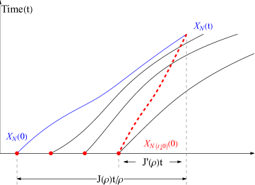
In this section, we deduce the conjecture on the limit fluctuation behaviour of end-point of backwards geodesic. There are essentially two terms appearing in the formula: the law of large number term and the fluctuation order term. For the law of large term, we have

$$X_{N(t\downarrow 0)}(0)-X_{N}(0)=\underbrace{X_{N}(t)-X_{N}(0)}_{=:\mathrm{I}}-\underbrace{(X_{N}(t)-X_{N(t\downarrow 0)}(0))}_{=:\mathrm{II}}.$$ (3.43)

By Definition, $J(\rho)$ is the expected rate of numbers of particles jumping across edge $\{0,1\}$, together with the density $\rho$, the law of large number term of ${\rm I}$ should be given as $J(\rho)t/\rho$. As for term ${\rm II},$ let $\rho(x,t)$ be the macroscopic particle’s density, then it should governed by [40, Equation (6.9)]

$$\frac{\partial\rho}{\partial t}=-\frac{\partial J(\rho)}{\partial x}=-\frac{\partial J(\rho)}{\partial\rho}\cdot\frac{\partial\rho}{\partial x}$$ (3.44)

so that $\rho$ is constant along the characteristic line $w(t)$ with $w(0)=\rho_{0}$ and $\frac{\partial w}{\partial t}=\frac{\partial J}{\partial\rho}$ [25]. On the other hand, the backwards geodesic mimics the characteristic line, thus, the law of large number term should be expressed as $J(\rho)t/\rho-J^{\prime}(\rho)t$, see Figure 5.

Refer to caption
Figure 5: The solid lines represent particle trajectories, with the blue line being the trajectory from which we construct the backward geodesic (the dashed red line). We have $X_{N(t\downarrow 0)}(0)-X_{N}(0)=X_{N}(t)-X_{N}(0)-(X_{N}(t)-X_{N(t\downarrow 0)}(0))$. Macroscopically, the first difference is about $\frac{J(\rho)t}{\rho}$, while the second difference is given by $J^{\prime}(\rho)t$.

For the fluctuation order term, by Conjecture 3.8, the correct order should be

$$C\Gamma(\rho)^{2/3}A(\rho)^{-1}t^{2/3}.$$ (3.45)

for some $C\in\mathbb{R}$. Comparing to the known result of TASEP, i.e., Theorem 2.6, we then obtain $C=2^{1/3}.$

Conjecture 3.9.

Consider any exclusion process with generator (2.2) and initial condition $X_{n}(0)=-\lfloor n/\rho\rfloor$ for some $\rho\in(0,1)$ such that its translation invariant stationary measure $\mu_{\rho}$ satisfies Assumption 3.7. Then666In both ASEP and ASEPsc, we have $J^{\prime}(\rho)=0$ for $\rho=1/2$. there exists universal constant $c_{2}$ such that

$$\lim_{t\to\infty}\frac{X_{N(t\downarrow 0)}(0)-X_{N}(0)-(J(\rho)/\rho-J^{\prime}(\rho))t}{2^{1/3}\Gamma(\rho)^{2/3}A(\rho)^{-1}t^{2/3}}\stackrel{{\scriptstyle d}}{{=}}\hat{u},$$ (3.46)

where $\hat{u}=\operatorname*{argmax}_{u\in\mathbb{R}}\left\{{\cal A}_{2}(u)-u^{2}\right\}$.

Scaling coefficients for the conjecture on ASEP

For ASEP, we can calculate

$$J(\rho)=(p-q)\rho(1-\rho),\quad A(\rho)=\rho(1-\rho),\quad\Gamma(\rho)=(p-q)/8.$$ (3.47)

Plugging $\rho=\tfrac{1}{2}$, we then obtain Conjecture 2.7.

Scaling coefficients for the conjecture on speed changed ASEP

For any $\rho\in[0,1]$, there exists an explicit stationary measure $\mu_{\rho}$ for ASEPsc as long as its jump rate satisfies

$$\begin{array}[]{lll}\alpha_{2}=e^{\beta}\alpha_{4},&\alpha_{2}+\alpha_{4}=2\alpha_{3},&\\[10.00002pt] \gamma_{2}=\alpha_{2}e^{-\beta}e^{-E},&\gamma_{3}=\alpha_{3}e^{-E},&\gamma_{4}=\alpha_{4}e^{\beta}e^{-E},\end{array}$$ (3.48)

for some $\beta,E\in\mathbb{R}$. Moreover, the stationary measure $\mu_{\rho}$ on $\{0,1\}^{\mathbb{Z}}$ of $\eta_{t}$ has the form [40, (6.19)]

$$\mu_{\rho}(\eta)=\frac{1}{Z}e^{\beta\sum_{i}\eta(i)\eta(i+1)+h\sum_{i}\eta(i)},$$ (3.49)

where $Z$ is the normalization constant and $h$ fixes the density. Defining

$$\mathfrak{h}(x,y)=e^{\beta xy+\frac{h}{2}(x+y)}$$ (3.50)

we then have

$$\mu_{\rho}(\eta)=\frac{1}{Z}\prod_{i}\mathfrak{h}(\eta(i),\eta(i+1)).$$ (3.51)

For initial condition with density $\rho=\tfrac{1}{2}$, $\mu_{\rho}$ satisfies Assumption 3.7. Recall that we set

$$\begin{array}[]{lll}\alpha_{2}=1,&\alpha_{3}=\frac{1}{2}\left(1+e^{-\beta}\right),&\alpha_{4}=e^{-\beta},\\[10.00002pt] \gamma_{2}=e^{-\beta}e^{-E},&\gamma_{3}=\frac{1}{2}\left(1+e^{-\beta}\right)e^{-E},&\gamma_{4}=e^{-E}.\end{array}$$ (3.52)

One can check that those parameter indeed satisfies condition (3.48). Hence, it remains to calculate $J(\rho)$ and $A(\rho)$. The choice of this model is due to the fact that, as mentioned in [40], it is one of the few growth model for which these model-dependent parameters can be computed analytically.

Lemma 3.10.

Let $\beta,E\in\mathbb{R}$ and $\rho\in[0,1]$ and jump rate given in (3.52). We have

$$J(\rho,\beta,E)=J_{+}(\rho,\beta)(1-e^{-E}),$$ (3.53)

where the positive current $J_{+}$ is given by

$$J_{+}(\rho,\beta)=\frac{2\rho(1-\rho)\left[e^{{\beta}}+\sqrt{(1-2\rho)^{2}+4\rho(1-\rho)e^{{\beta}}}\right]}{e^{{\beta}}\left[1+\sqrt{(1-2\rho)^{2}+4\rho(1-\rho)e^{{\beta}}}\right]^{2}}.$$ (3.54)

Its integrated covariance is given by

$$A(\rho,\beta,E)=\rho(1-\rho)\sqrt{(1-2\rho)^{2}+4\rho(1-\rho)e^{\beta}}.$$ (3.55)

Plugging this with $\rho=\tfrac{1}{2}$ into Lemma 3.10 leads to (2.24). Applying Conjecture 3.8 (resp. Conjecture 3.9), we then obtain Conjecture 2.9 (resp. Conjecture 2.8). Hence, it remains to prove Lemma 3.10. First note that the measure $\mu_{\rho}$ in (3.51) satisfies spatial Markov property.

Lemma 3.11.

For any $n\in\mathbb{Z}_{\geq 1}$ and $\eta\in\{0,1\}^{\mathbb{Z}}$, it holds

$$\mu_{\rho}(\eta(n)|\eta(0),\ldots,\eta(n-1))=\mu_{\rho}(\eta(n)|\eta(n-1)).$$ (3.56)
Proof.

Let $m,n\in\mathbb{Z}$ with $m\leq n$ and $\eta(m),\ldots,\eta(n)\in\{0,1\}$. We also define

$\displaystyle\mathbb{Z}_{<n}=\{x\in\mathbb{Z}|x<n\},\quad\mathbb{Z}_{>n}=\{x\in\mathbb{Z}|x>n\},\quad\forall n\in\mathbb{Z}.$ (3.57)

By (3.51), we have

$\displaystyle\mu_{\rho}(\eta(m),\ldots,\eta(n))$ (3.58)
$\displaystyle=$ $\displaystyle\frac{1}{Z}\sum_{\xi_{1}\in\{0,1\}^{\mathbb{Z}_{<m}}}\sum_{\xi_{2}\in\{0,1\}^{\mathbb{Z}_{>n}}}\left\{\bigg{(}\prod_{i<m-1}\mathfrak{h}(\xi_{1}(i),\xi_{1}(i+1))\!\bigg{)}\mathfrak{h}(\xi_{1}(m-1),\eta(m))\right.$
$\displaystyle\times$ $\displaystyle\left.\bigg{(}\prod_{i=m}^{n-1}\mathfrak{h}(\eta(i),\eta(i+1))\!\bigg{)}\mathfrak{h}(\eta(n),\xi_{2}(n+1))\prod_{i>n}\mathfrak{h}(\xi_{2}(i),\xi_{2}(i+1))\right\}$

which can be further written as

$\displaystyle\underbrace{\frac{1}{\sqrt{Z}}\sum_{\xi_{1}\in\{0,1\}^{\mathbb{Z}_{<m}}}\bigg{(}\prod_{i<m-1}\mathfrak{h}(\xi_{1}(i),\xi_{1}(i+1))\!\bigg{)}\mathfrak{h}(\xi_{1}(m-1),\eta(m))}_{=:L(m,\eta(m))}$ (3.59)
$\displaystyle\times\bigg{(}\prod_{i=m}^{n-1}\mathfrak{h}(\eta(i),\eta(i+1))\!\bigg{)}\underbrace{\frac{1}{\sqrt{Z}}\sum_{\xi_{2}\in\{0,1\}^{\mathbb{Z}_{>n}}}\!\!\!\mathfrak{h}(\eta(n),\xi_{2}(n+1))\bigg{(}\prod_{i>n}\mathfrak{h}(\xi_{2}(i),\xi_{2}(i+1))\!\bigg{)}}_{=:R(\eta(n),n)}.$

Thus we have

$\displaystyle\mu_{\rho}(\eta(n)|\eta(0),\ldots,\eta(n-1))=\frac{\mu_{\rho}(\eta(0),\ldots,\eta(n))}{\mu_{\rho}(\eta(0),\ldots,\eta(n-1))}$ (3.60)
$\displaystyle=$ $\displaystyle h(\eta(n-1),\eta(n))\frac{R(\eta(n),n)}{R(\eta(n-1),n-1)}=\frac{\mu_{\rho}(\eta(n-1),\eta(n))}{\mu_{\rho}(\eta(n-1))}=\mu_{\rho}(\eta(n)|\eta(n-1)),$

which completes the proof. ∎

This result implied in particular that

$$\mu_{\rho}(\eta(m),\ldots,\eta(n))=\mu_{\rho}(\eta(m))\prod_{i=m}^{n-1}\mu_{\rho}(\eta(i+1)|\eta(i)),\quad\forall m,n\in\mathbb{Z}$$ (3.61)

allowing us to compute $J(\rho)$ and $A(\rho)$ as follows.

Proof of Lemma 3.10.

The stationary current. By its definition, see (3.37), we have

$$J(\rho,\beta,E)=\underbrace{\sum_{\begin{subarray}{c}\eta\in\Omega\\ \eta(0)=1,\eta(1)=0\end{subarray}}c_{\eta}(0,1)\mu_{\rho}(\eta)}_{=:J_{+}(\rho,\beta)}-\underbrace{\sum_{\begin{subarray}{c}\eta\in\Omega\\ \eta(0)=0,\eta(1)=1\end{subarray}}c_{\eta}(1,0)\mu_{\rho}(\eta)}_{=:J_{-}(\rho,\beta)}.$$ (3.62)

By the definition of jump rate (2.5), we have

$\displaystyle J_{+}(\rho,\beta)$ $\displaystyle=\alpha_{2}\mu_{\rho}(\eta(-1)=0,\eta(0)=1,\eta(1)=0,\eta(2)=1)$ (3.63)
$\displaystyle+\alpha_{3}\mu_{\rho}(\eta(-1)=1,\eta(0)=1,\eta(1)=0,\eta(2)=1)$
$\displaystyle+\alpha_{3}\mu_{\rho}(\eta(-1)=0,\eta(0)=1,\eta(1)=0,\eta(2)=0)$
$\displaystyle+\alpha_{4}\mu_{\rho}(\eta(-1)=1,\eta(0)=1,\eta(1)=0,\eta(2)=0).$

Set

$$\hat{\alpha}=\mu_{\rho}(\eta(1)=1|\eta(0)=0),\quad\hat{\beta}=\mu_{\rho}(\eta(1)=0|\eta(0)=1).$$ (3.64)

Applying (3.52), translation invariance and spatial Markov property (3.61) to (3.63), we obtain

$\displaystyle J_{+}(\rho,\beta)=$ $\displaystyle(1-\rho)\hat{\alpha}\hat{\beta}\hat{\alpha}+\frac{1+e^{-\beta}}{2}\rho(1-\hat{\beta})\hat{\beta}\hat{\alpha}$ (3.65)
$\displaystyle+\frac{1+e^{-\beta}}{2}(1-\rho)\hat{\alpha}\hat{\beta}(1-\hat{\alpha})+\rho(1-\hat{\beta})\hat{\beta}(1-\hat{\alpha})e^{-\beta}.$

Similarly, we get $J_{-}(\rho,\beta)=e^{-E}J_{+}(\rho,\beta)$, which then implies

$$J(\rho,\beta,E)=(1-e^{-E})J_{+}(\rho,\beta).$$ (3.66)

To show (3.54), we need to express $\hat{\alpha},\hat{\beta}$ in terms of $\rho$ and $\beta$. Note that

$\displaystyle 1-\rho$ $\displaystyle=\mu_{\rho}(\eta(k+1)=0)$ (3.67)
$\displaystyle=\mu_{\rho}(\eta(k+1)=0|\eta(k)=1)\mu_{\rho}(\eta(k)=1)$
$\displaystyle\quad+\mu_{\rho}(\eta(k+1)=0|\eta(k)=0)\mu_{\rho}(\eta(k)=0)$
$\displaystyle=\hat{\beta}\rho+(1-\hat{\alpha})(1-\rho),$

which then implies

$$\rho=\frac{\hat{\alpha}}{\hat{\alpha}+\hat{\beta}}.$$ (3.68)

On the other hand, by spatial Markov property (3.61), we have

$\displaystyle\mu_{\rho}(\eta(0),\eta(1),\ldots)=\mu_{\rho}(\eta(0))\prod_{i=0}^{\infty}\mu_{\rho}(\eta(i+1)|\eta(i))$ (3.69)
$\displaystyle=$ $\displaystyle(1-\rho)^{1-\eta(0)}\rho^{\eta(0)}\prod_{i=0}^{\infty}(1-\hat{\alpha})^{(1-\eta(i))(1-\eta(i+1))}\hat{\alpha}^{(1-\eta(i))\eta(i+1)}\hat{\beta}^{\eta(i)(1-\eta(i+1))}(1-\hat{\beta})^{\eta(i)\eta(i+1)}$
$\displaystyle=$ $\displaystyle{\rm const}\times\prod_{i=0}^{\infty}\bigg{[}\frac{\hat{\alpha}\hat{\beta}}{(1-\hat{\beta})(1-\hat{\alpha})}\bigg{]}^{\eta(i)\eta(i+1)}\bigg{[}\frac{\hat{\alpha}\hat{\beta}}{(1-\hat{\alpha})^{2}}\bigg{]}^{\eta(i)}.$

Comparing this with (3.49) we obtain

$$e^{-\beta}=\frac{\hat{\alpha}\hat{\beta}}{(1-\hat{\beta})(1-\hat{\alpha})}.$$ (3.70)

Combining (3.68) and (3.70), we finally get

$$\hat{\alpha}=\frac{2\rho}{1+\sqrt{(1-2\rho)^{2}+4\rho(1-\rho)e^{\beta}}},\quad\hat{\beta}=\frac{1-\sqrt{(1-2\rho)^{2}+4\rho(1-\rho)e^{\beta}}}{2\rho(1-\gamma)}.$$ (3.71)

Plugging (3.71) back into (3.63) and (3.66), we get the claimed expression for the stationary current.

The integrated stationary covariance. Applying translation invariance and the definition of the integrated covariance, see (3.38), we have

$\displaystyle A(\rho,\beta,E)=$ $\displaystyle\sum_{j\in\mathbb{Z}}(\mu_{\rho}(\eta(0)\eta(j))-\rho^{2})=\sum_{j\in\mathbb{Z}}(\mu_{\rho}(\eta(0)=\eta(j)=1)-\rho^{2})$ (3.72)
$\displaystyle=$ $\displaystyle\rho-\rho^{2}+2\sum_{j\geq 1}^{\infty}(\mu_{\rho}(\eta(0)=\eta(j)=1)-\rho^{2})$
$\displaystyle=$ $\displaystyle\rho(1-\rho)+2\sum_{j\geq 1}^{\infty}(\mu_{\rho}(\eta(j)=1|\eta(0)=1)\rho-\rho^{2}),$

Choose a fixed $j>0$, by (3.56), we can consider $(\eta(n))_{n\in\mathbb{Z}_{>0}}$ as a spatial Markov chain with transition matrix

$$T=\begin{pmatrix}1-\hat{\alpha}&\hat{\alpha}\\ \hat{\beta}&1-\hat{\beta}\end{pmatrix},$$ (3.73)

where $\hat{\alpha},\hat{\beta}$ are the same as (3.64). Then we have

$$\mu(\eta(j)=1|\eta(0)=1)=[T^{j}]_{1,1},$$ (3.74)

where $[T^{j}]_{1,1}$ is the component of matrix $T^{j}$ on first column and row. Applying eigenbasis decomposition, we have $T=U\hat{T}U^{-1}$, where

$$U=\begin{pmatrix}1&-\hat{\alpha}\\ 1&\hat{\beta}\end{pmatrix},\quad\hat{T}=\begin{pmatrix}1&0\\ 0&1-\hat{\alpha}-\hat{\beta}\end{pmatrix},$$ (3.75)

which implies

$$\mu(\eta(j)=1|\eta(0)=1)=\rho+(1-\rho)(1-\hat{\alpha}-\hat{\beta})^{j},\quad\forall j\in Z_{\geq 1}.$$ (3.76)

Plugging this into (3.72), we have

$\displaystyle A(\rho,\beta,E)=$ $\displaystyle\rho(1-\rho)+2\sum_{j=1}^{\infty}(1-\rho)(1-\hat{\alpha}-\hat{\beta})^{j}$ (3.77)
$\displaystyle=$ $\displaystyle\rho(1-\rho)\bigg{(}1+\frac{2(1-\hat{\alpha}-\hat{\beta})}{\hat{\alpha}+\hat{\beta}}\bigg{)}.$

Replacing $\hat{\alpha},\hat{\beta}$ we obtained the claimed formula. ∎

4 Simulation results

In this section, we present the numerical results. The raw data can be found in the BonnData repository [29]. Recall that for a random variable $Y$, the skewness and kurtosis are defined as

$$\mathrm{Skew}(Y)=\frac{\mathbb{E}\left((Y-\mu)^{3}\right)}{\mathbb{E}\left((Y-\mu)^{2}\right)^{3/2}},\quad\mathrm{Kurt}(Y)=\frac{\mathbb{E}\left((Y-\mu)^{4}\right)}{\mathbb{E}\left((Y-\mu)^{2}\right)^{2}},$$ (4.1)

where $\mu=\mathbb{E}(Y)$. Moreover, we denote

$$\overline{\mathbb{E}}(Y)=\frac{1}{n}\sum_{i=1}^{n}y_{i},$$ (4.2)

as its empirical expectation (we also use similar notation for other statistics: variance, skewness, and kurtosis), where $y_{1},y_{2},\ldots,y_{n}$ are independent realizations of the random variable $Y$.

4.1 Results for ASEP

4.1.1 End-point of backwards geodesic
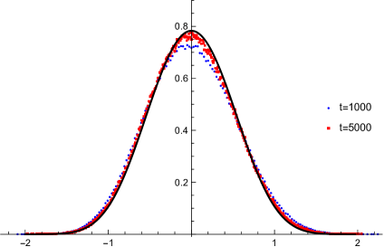
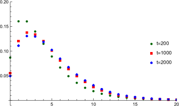
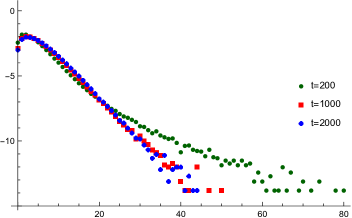
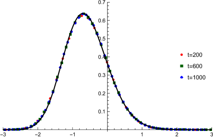
We have simulated ASEP with $p=3/4$, which is far away from the TASEP case ($p=1$) and the SSEP (symmetric simple exclusion process) case ($p=1/2$). In Figure 6, we compare the empirical density function of $B_{t}^{{\rm ASEP}}$ at times $t=1000$ and $t=5000$ with the density function of $\hat{u}$. For increasing time, the empirical density function of $B_{t}^{{\rm ASEP}}$ converges to the density function of $\hat{u}$.

Refer to caption
Figure 6: Comparison between the density function of $B_{t}^{\rm ASEP}$ and $\hat{u}$. The black line represents the probability density function of $\hat{u}$, while the red (resp. blue) points correspond to the probability density of $B_{t}^{\rm ASEP}$ at time $t=1000$ (resp. $t=5000$). The number of trials is $10^{6}$.

The convergence to $\hat{u}$ is confirmed at the level of the first three standard statistics. Indeed, denote by $\overline{\mathbb{E}}(B_{t_{i}}^{{\rm ASEP}})$ the empirical mean of $B_{t_{i}}^{{\rm ASEP}}$, and

$$\widehat{\mathbb{E}}\left(B_{t_{i}}^{{\rm ASEP}}\right)=\left|\overline{\mathbb{E}}(B_{t_{i}}^{{\rm ASEP}})-\mathbb{E}\left(\hat{u}\right)\right|,$$ (4.3)

and similarly for other statistics: ${\rm Var}$, ${\rm Skew}$, and ${\rm Kurt}$.

Refer to caption
Figure 7: Log-log plot for the statistics of $B_{t}^{\mathrm{ASEP}}$. The square, triangle, and circle markers represent the points corresponding to $(t_{i},\widehat{\mathbb{E}}(B_{t}^{\mathrm{ASEP}}))$, $(t_{i},\widehat{\mathrm{Var}}(B_{t}^{\mathrm{ASEP}}))$, and $(t_{i},\widehat{\mathrm{Skew}}(B_{t}^{\mathrm{ASEP}}))$, respectively, where $t_{i}\in\{1000,1500,\ldots,5000\}$. The blue, red, and black solid lines are the reference lines $(t,t^{-1/3})$, $(t,4t^{-2/3})$, and $(t,0.045t^{-1/3})$, respectively. The number of trials is $10^{6}$.

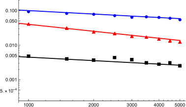
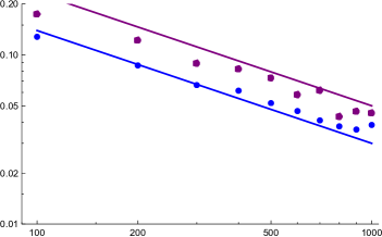
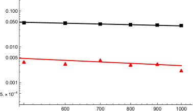
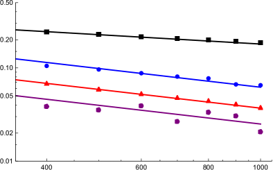
In Figure 7 we have a log-log plot of these statistics and we clearly see that in all cases the convergence to the ones of $\hat{u}$ are power-law. More precisely, $\widehat{\mathbb{E}}\left(B_{t_{i}}^{{\rm ASEP}}\right)$ and $\widehat{\mathrm{Skew}}(B_{t}^{\mathrm{ASEP}})$ converges to 0 as $t^{-1/3}$, while the speed of convergence $\widehat{\mathrm{Var}}(B_{t}^{\mathrm{ASEP}})$ is $t^{-2/3}$. As often is the case, the statistics of the kurtosis is much more noisy and it did not provide reliable numbers, so we did not include in the plot.

4.1.2 On the discrepancy $D_{N}(t)$

Next, we provide numerical evidence that the discrepancy $D_{n}(t)$ tends to a random variable without scaling in time. In the left panel of Figure 8, we illustrate the empirical density function of $D_{n}(t)$ at $t=200$, $t=1000$, and $t=2000$, while in the right panel of Figure 8 we show the log-linear plots of it. As time increases, one observes that the probability of the very small values of $D_{N}(t)$ slightly decreases, but more importantly, the probabilities of the large values considerably decrease, indicating that $D_{N}(t)$ tends to a random variable.

Refer to caption
Refer to caption
Figure 8: Probability density function $f_{D_{n}(t)}$ in ASEP with $p=3/4$. Left panel: Original density function $(x,f_{D_{n}(t)}(x))$. Right panel: Log-linear plot $(x,\log f_{D_{n}(t)}(x))$. The green, red, and blue points in the figure correspond to $t=200$, $t=1000$, and $t=2000$, respectively. The number of trials is $10^{6}$.

We also present the statistics of $D_{n}(t)$ at times $t=400,800,\dots,2000$ in Table 1. The expectation and variance slightly increase with time, and the skewness decreases over time. However, the rates of change are extremely slow, and The rate of change is gradually slowing down over time. As for the kurtosis, compared to the other statistics, it appears to exhibit greater numerical instability.

$t$ $\mathbb{E}\left(D_{N}(t)\right)$ $\operatorname{Var}\left(D_{N}(t)\right)$ $\operatorname{Skew}\left(D_{N}(t)\right)$ $\operatorname{Kurt}\left(D_{N}(t)\right)$
$400$ 4.34 12.96 1.80 9.73
$800$ 4.62 13.10 1.47 6.79
$1200$ 4.79 13.57 1.41 6.33
$1600$ 4.88 13.81 1.38 6.15
$2000$ 4.95 14.07 1.34 5.88
Table 1: Empirical mean, variance, skewness, and kurtosis of the discrepancy $D_{n}(t)$ with $t\in\{400,800,\ldots,2000\}$. The number of trials is $10^{6}$.

4.2 Results for speed changed ASEP

4.2.1 Fluctuations of tagged particle position

We made the simulation of the ASEPsc with jump rate given by (2.22) with parameters $\beta=\log 4$ and $E=\infty$ (particles can only jump to right). Denote $X_{{\rm GOE}}$ as a random variable such that

$$\mathbb{P}\left(X_{{\rm GOE}}\leq s\right)=F_{{\rm GOE}}(2s).$$ (4.4)

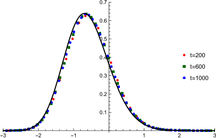
In Figure 9, we compare the empirical density function of $X^{\rm resc}_{N}(t)$ at times $t=200$, $t=600$, and $t=1000$ with the density function of $X_{{\rm GOE}}$. One clearly see that the shape of the two functions are very close, indicating that $X^{\rm resc}_{N}(t)$ indeed converges in distribution to $X_{{\rm GOE}}$. Also, one can see a slight shift to the right, which decreases over time. This is a general fact occurring in models in the KPZ class as discussed in Remark 4.1 below.

Refer to caption
Figure 9: Numerical verification for Conjecture 2.9. The red, green, and blue dots represent the density function of $X^{\rm resc}_{n}(t)$ with $t\in\{200,600,1000\}$. The black solid line is given by $(s,2F^{\prime}_{\rm GOE}(2s))$. The number of trials is $10^{6}$.

We use the same notation as in (4.3), that is,

$$\widehat{\mathbb{E}}\left(X^{\rm resc}_{N}(t)\right)=\left|\overline{\mathbb{E}}(X^{\rm resc}_{N}(t))-\mathbb{E}\left(X_{{\rm GOE}}\right)\right|$$ (4.5)

and also for other statistics. To illustrate the convergence, we show in Figure 10 the log-log plots of these statistics as a function of time. The reference line for the expectation has slope $-1/3$, while for the other three statistics the slope is $-2/3$. Thus the speed of convergence of the expectation of $X^{\rm resc}_{N}(t)$ is $\mathcal{O}(t^{-1/3})$, whereas for the other three statistics is $\mathcal{O}(t^{-2/3})$.

Refer to caption
Refer to caption
Figure 10: Log-log plot for the absolute difference between the statistics of $X^{\rm resc}_{N}(t)$ and $X_{{\rm GOE}}$. Left panel: The pentagon represents $\widehat{\mathrm{Kurt}}(X^{\rm resc}_{N}(t))$ and the circle represents $\widehat{\mathrm{Skew}}(X^{\rm resc}_{N}(t))$. The purple solid line is the reference line $(t,5t^{-2/3})$, and the blue line is $(t,3t^{-2/3})$. Right panel: The rectangle represents $\widehat{\mathrm{Var}}(X^{\rm resc}_{N}(t))$ and the triangle represents $\widehat{\mathbb{E}}(X^{\rm resc}_{N}(t))$. The black solid line is the reference line $(t,5t^{-1/3}/13)$, and the red line is $(t,3t^{-2/3}/10)$. The number of trials is $10^{6}$.
Remark 4.1.

In the unscaled variables, the mean has a shift of order one, which is typical for models in the KPT universality class, see [55, 56] for real experimental results, and [27] for theoretical results. In our case, since the slope of the black line in Figure 10 is about $0.38(5)$, so we define

$$\hat{X}^{\rm resc}_{N}(t)=\frac{X_{N}^{{\textrm{ASEPsc}}}(t)-X^{\textrm{ASEPsc}}_{N}(0)-2J(\beta,E)t+0.385}{-2\Gamma(\beta,E)^{1/3}t^{1/3}}.$$ (4.6)

Then one observes better convergence behavior since now also the expectation converges at speed $t^{-2/3}$, see Figure 11 compared to Figure 9.

Refer to caption
Figure 11: The red, green, and blue dots represent the density function of $\widehat{X}^{\rm resc}_{n}(t)$ with $t\in\{200,600,1000\}$. The black solid line is given by $(s,2F^{\prime}_{\rm GOE}(2s))$. The number of trials is $10^{6}$.

4.2.2 End-point of backwards geodesic

By the construction of the backwards geodesic on particles, even for density $\rho=1/2$, the law of the starting point is not symmetric unlike the law of $\hat{u}$. However as we numerically see, this asymmetry asymptotically will disappear. The asymmetry would not be present for $\rho=1/2$ if one would have considered the backwards geodesic for height functions as for example in [18].

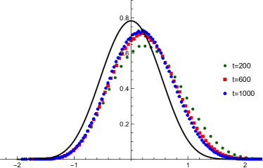
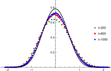
In Figure 12, we present a comparison of the empirical density function of $B^{{\rm ASEPsc}}_{t}$ defined in (2.23) at times $t=200$, $t=600$, and $t=1000$ with the density function of $\hat{u}$. From the probability density plot, we observe that as time increases, the density function of $B^{{\rm ASEPsc}}_{t}$ slowly approaches that of $\hat{u}$. As the empirical mean is converging quite slowly (see below) we also plot the density function of the centered version of $B^{{\rm ASEPsc}}_{t}$, that is,

$$\hat{B}^{{\rm ASEPsc}}_{t}=B^{{\rm ASEPsc}}_{t}-\overline{\mathbb{E}}\left(B^{{\rm ASEPsc}}_{t}\right).$$ (4.7)

In the right panel of Figure 12 one better sees the convergence trend over time.

Refer to caption
Refer to caption
Figure 12: Numerics for Conjecture 2.8. Left panel: The green, red, and blue dots represent the density function of $B_{t}^{{\rm ASEPsc}}$ with $t\in\{200,600,1000\}$. Right panel: The green, red, and blue dots represent the density function of $\hat{B}_{t}^{{\rm ASEPsc}}$ with $t\in\{200,600,1000\}$. The black solid line is the density function of $\hat{u}$. The number of trials is $10^{6}$.

For ASEPsc the convergence is slower than for ASEP and thus it is even more important to look at the convergence of the statistics. Recall the notations as in (4.3), $\widehat{\mathbb{E}}\left(B^{{\rm ASEPsc}}_{t}\right)=\left|\overline{\mathbb{E}}(B^{{\rm ASEPsc}}_{t})-\mathbb{E}\left(\hat{u}\right)\right|$ and similarly for the other statistics. In Figure 13, we plot the log-log plots of the first four statistics as compared with the ones of $\hat{u}$. We see that the expectation of $B^{{\rm ASEPsc}}_{t}$ converges as $t^{-1/3}$, while the other three statistics converges faster, namely as $t^{-2/3}$.

Refer to caption
Figure 13: Log-log plot for the statistic of $B^{{\rm ASEPsc}}_{t}$. The rectangle, triangle, circle, and pentagon represent the numerical values of $\widehat{\mathbb{E}}(B^{{\rm ASEPsc}}_{t})$, $\widehat{\mathrm{Var}}(B^{{\rm ASEPsc}}_{t})$, $\widehat{\mathrm{Skew}}(B^{{\rm ASEPsc}}_{t})$, and $\widehat{\mathrm{Kurt}}(B^{{\rm ASEPsc}}_{t})$, respectively. The black, blue, red, and purple solid lines are the reference lines $(t,1.8t^{-1/3})$, $(t,6.2t^{-2/3})$, $(t,3.7t^{-2/3})$, and $(t,2.5t^{-2/3})$, respectively. The number of trials is $10^{6}$.

Appendix A Numerical implementation

A.1 Implementation for $\operatorname*{argmax}_{u\in\mathbb{R}}\{{\cal A}_{2}(u)-u^{2}\}$

The implementation of distribution of $\hat{u}=\operatorname*{argmax}\{{\cal A}_{2}(u)-u^{2}\}$ is based on the formula in777Another formula is obtained in [50], and it was shown in [3] that they are the same. [35]. Let ${\rm Ai}$ be Airy function and operator $P_{0}$ as the projection on positive real line, i.e., $P_{0}f(x)=\mathbbm{1}_{x>0}f(x)$. For $t,m\in\mathbb{R}$, define the functions

$\displaystyle B_{m}(x,y)$ $\displaystyle=\mathrm{Ai}(x+y+m),$ (A.1)
$\displaystyle\psi_{t,m}(x)$ $\displaystyle=2e^{xt}\left[t\mathrm{Ai}\left(x+m+t^{2}\right)+\mathrm{Ai}^{\prime}\left(x+m+t^{2}\right)\right]$

and the kernel

$$\Psi_{t,m}(x,y)=2^{1/3}\psi_{t,m}\left(2^{1/3}x\right)\psi_{-t,m}\left(2^{1/3}y\right).$$ (A.2)

Define also $\mathcal{M}=\max_{u\in\mathbb{R}}\{{\cal A}_{2}(u)-u^{2}\}$, the joint density of $(\hat{u},\mathcal{M})$ is [35, Theorem 2]:

$\displaystyle f(t,m)=\det\left(\mathbbm{1}-P_{0}B_{4^{1/3}}P_{0}+P_{0}\Psi_{t,m}P_{0}\right)-F_{\mathrm{GOE}}\left(4^{1/3}m\right),$ (A.3)

where $F_{\mathrm{GOE}}$ is GOE Tracy-Widom distribution. Both quantities on the right hand side of (A.3) can be obtained numerically via Bornemann’s method [14]. Integrating over $\mathcal{M}$, one obtains the distribution of $\hat{u}$.

A.2 Implementation for ASEP

Denote the total simulation time as $t_{\max}$ and the number of particles as $N_{\max}$. In the implementation we set $t_{\max}=5000$ and $N_{\max}=3750$ and the index of particle from where we construct backwards geodesic is given by $N=937$. The total number of trials is $10^{6}$. For a fixed realization of $X(t_{\max})$, we will record $N(t_{i}\downarrow 0)$ with $t_{i}\in\{500,1000,\ldots,5000\}$.

A.2.1 For original process

The initial condition is888In the simulation we used a left-to-right ordering unlike formulas in the theoretical part of this paper. $X_{n}(0)=2n-1$ for $n\in\{1,\ldots,N\}$. We will first prepare three random matrices $\mathcal{J},\mathcal{U},\mathcal{D}\in\mathcal{R}_{\geq 0}^{N\times C_{N}t_{\max}}$ for some $C_{N}>0$ depending on $N$ in the following way:

  1. 1.

    $\mathcal{J}_{i,j}\sim{\rm Exp}(1)$ are i.i.d. random variables. Column $n$ of this matrix provides the information when particle $X_{n}$ will attempt to jump: the $m-$the attempted jump time of particle $X_{n}$ is $\sum_{i=1}^{m}\mathcal{J}_{i,n}$.

  2. 2.

    $\mathcal{U}_{i,j}\sim{\rm Unif}([0,1])$ are i.i.d. random variables and

    $$\mathcal{D}_{i,j}=\begin{cases}1,\quad&\mathrm{if}\ \mathcal{U}_{i,j}\leq p,\\ -1,&\mathrm{otherwise}.\end{cases}$$ (A.4)

    The $n-$th column of $\mathcal{D}$ tells us in which direction particle $X_{n}$ should attempt to jump: if $\mathcal{D}_{m,n}=1$, then the dirction of $m-$th attempted jump of particle $X_{n}$ is from left to right otherwise from right to left.

In the simulation, we will choose $C_{N}$ (depending on $N$) large enough such that $\min_{n}\{\sum_{i=1}^{C_{N}t_{\max}}\mathcal{J}_{i,n}\}\geq t_{\max}$ with high probability. For a given initial condition $X(0)$ and matrices $\mathcal{J},\mathcal{D}$, the final state $X(t)$ is a deterministic result. We record current particle’s time-space position in two vectors $\mathcal{S},\mathcal{T}\in\mathcal{R}_{\geq 0}^{N+1}$ with $\mathcal{T}_{1}=\mathcal{T}_{N+1}=t_{\max}$ and $\mathcal{S}_{N+1}=\infty$. The information about next attempted jump direction is stored in vector ${\cal A}\in\{-1,1\}^{N}$. The updating rule is as follows:

  1. 1.

    Inital step: Set $\mathcal{S}_{n}=X_{n}(0)$, $\mathcal{T}_{n}=\mathcal{J}_{1,n}$, ${\cal A}_{n}=\mathcal{D}_{1,n}$ and $\mathcal{H}_{n}=2$ for all $n\in\{1,\ldots,N\}$.

  2. 2.

    Induction step: For given $\mathcal{S},\ \mathcal{T},\ {\cal A}$ and $\mathcal{H}$, until $\min\{\mathcal{T}_{n}\}\geq t_{\max}$, we choose $m\in\{2,\ldots,N\}$ such that $\mathcal{T}_{m}\leq\min\{\mathcal{T}_{m+1},\mathcal{T}_{m-1}\}$ and update

    $$\mathcal{S}_{m}=\begin{cases}\mathcal{S}_{m}+1,\quad&\mathrm{if}\ {\cal A}_{m}=1\ \mathrm{and}\ \mathcal{S}_{m+1}\neq\mathcal{S}_{m}+1,\\ \mathcal{S}_{m}-1,\quad&\mathrm{if}\ \mathcal{D}_{m}=-1\ \mathrm{and}\ \mathcal{S}_{m-1}\neq\mathcal{S}_{m}-1,\\ \mathcal{S}_{m},&\mathrm{otherwise.}\end{cases}$$ (A.5)

    We also update its current time position as $\mathcal{T}_{m}=\mathcal{T}_{m}+\mathcal{J}_{\mathcal{H}_{m},m}$. In the case when ${\cal A}_{m}=1$ and $\mathcal{S}_{m+1}=\mathcal{S}_{m}+1$ (resp. ${\cal A}_{m}=-1$ and $\mathcal{S}_{m-1}=\mathcal{S}_{m}-1$), this jump will be recorded as suppressed left to right jump (resp. right to left jump). Updated ${\cal A}_{m}=\mathcal{D}_{\mathcal{H}_{m},m}$ and $\mathcal{H}_{m}=\mathcal{H}_{m}+1$.

A.2.2 For backwards geodesic

Along the construction of ASEP, the information about the suppressed left to right (resp. right to left) jumps will be stored in matrix $\mathcal{T}^{\not\rightarrow}$ (resp. $\mathcal{T}^{\not\leftarrow}$): $\mathcal{T}_{i,n}^{\not\rightarrow}$ is the time of $i-$th suppressed left to right jump of particle $X_{n}$. For a given time $t\in[0,t_{\max}]$ and $n\in\{1,\ldots,N\}$, the end-point of backwards geodesic of particle $X_{n}$ is obtained as follows:

  1. 1.

    Initial step: At time $t$, we set $N(t\downarrow t)=n$.

  2. 2.

    Induction step: Given $m=N(t\downarrow s)$, find $\tau=\max\{r\leq s|r\in\mathcal{T}^{\not\rightarrow}_{m}\cup\mathcal{T}^{\not\leftarrow}_{m}\}$. If $\tau\in\mathcal{T}_{m}^{\not\rightarrow}$ (resp. $\tau\in\mathcal{T}^{\not\leftarrow}$), then update $N(t\downarrow\tau)=m+1$ (resp. $N(t\downarrow\tau)=m-1$).

A.2.3 For discrepancy in ASEP

For a given $t\in[0,t_{\max}]$ and $n\in\{1,\ldots,N\}$, after obtaining $N(t\downarrow 0)$ described as above, we will implement $D_{n}(t)$ defined in (2.13) as follows:

  1. 1.

    Consider a new ASEP $\hat{X}(t)$ with initial condition given by $\hat{X}_{j}(0)=X_{N(t\downarrow 0)}(0)-(N(t\downarrow 0)-j)$ for all $j\leq N(t\downarrow 0)$.

  2. 2.

    The time evolution follows the same realization of random matrices $\mathcal{J}$ and $\mathcal{D}$ as the one for original process $X(t)$: for $n\leq N(t\downarrow 0)$, $\mathcal{J}_{i,j}$ (resp. $\mathcal{D}_{i,j}$) is the $i-$th attempted jump time (resp. the direction of $i-$th attempted jump) of particle $\hat{X}_{j}$.

Then $D_{n}(t)$ in (2.13) is given by $\hat{X}_{n}(t)-X_{n}(t)$. Due to the high time consuming of the simulation, here we choose $t_{\max}=2000$ and $N_{\max}=1500$. The total number of trials is $10^{6}$. The index of particle from where we constructed backwards geodesic is given $N=375$. For each realization of $X(t)$, we construct $\hat{X}(t_{i})$ with $t_{i}\in\{200,400,\ldots,2000\}$.

A.3 Implementation for speed changed

Due to the absence of homogeneity of jump rate, the implementation of ASEPsc is slightly different from the one for ASEP, namely, it does not make sense to prepare matrices $\mathcal{J},\mathcal{D}$ once for all time as we did for ASEP. The jump rates illustrated in Figure 2 do not include the situations of suppressed jumps. In the same spirit of ASEP, also for ASEPsc we assign jump trials from $j$ to $j+1$ (resp. from $j+1$ to $j$) as in Figure 2 without at first caring whether the arrival site is occupied or empty. If the arrival site for right jumps at $j+1$ (resp. left jumps at $j$) is occupied, the it will be a suppressed jump.

For given jump rate, we then determine $X(t)$ as follows:

  1. 1.

    Initial step:

    1. (a)

      For space-time trajectory: set $\mathcal{S}_{n}=2n-1$ and $\mathcal{T}_{n}=0$ for all $n$.

    2. (b)

      For jump schema: For each $n\in\{1,\ldots,N\},$ we find its left (resp. right) jump rate $\theta^{n}_{\ell}$ (resp. $\theta^{n}_{r}$) according to its local environment. Define $\mathcal{R}_{n}=\theta_{\ell}^{n}+\theta_{r}^{n}$.

    3. (c)

      For probability being chosen: Let $\mathcal{P}_{n}=(\sum_{i=1}^{n}\mathcal{R}_{i})/(\sum_{i=1}^{N}\mathcal{R}_{i})$ for all $n\geq 1$ and $\mathcal{P}_{0}=0$.

  2. 2.

    Induction step: For given $\mathcal{S},\ \mathcal{T},\ \mathcal{R}$ and $\mathcal{P}$, until $\min_{n}\{\mathcal{T}_{n}\}\geq t_{\max}$, we let $\mathcal{U}\sim{\rm Unif}([0,1])$ and find $m\in\{1,\ldots,N\}$ such that $\mathcal{P}_{m-1}<\mathcal{U}\leq\mathcal{P}_{m}$. Then we update the $\mathcal{S},\ \mathcal{T},\ \mathcal{R}$ and $\mathcal{P}$ as follows:

    1. (a)

      For time position: Set $\mathcal{T}_{n}=\mathcal{T}_{n}+\mathcal{J}$, where $\mathcal{J}\sim{\rm Exp}(\mathcal{R}_{m})$ for all $n$.

    2. (b)

      For space position: Let $\mathcal{K}\sim Unif([0,1])$ be i.i.d. and set

      $$\mathcal{S}_{m}=\begin{cases}\mathcal{S}_{m}+1,\quad&\mathrm{if}\ \mathcal{K}_{m}\leq\frac{\theta_{r}^{m}}{\theta_{\ell}^{m}+\theta_{r}^{m}}\ \mathrm{and}\ \mathcal{S}_{n+1}>\mathcal{S}_{m}+1,\\ \mathcal{S}_{m}-1,&\mathrm{if}\ \mathcal{K}_{m}>\frac{\theta_{r}^{m}}{\theta_{\ell}^{m}+\theta_{r}^{m}}\ \mathrm{and}\ \mathcal{S}_{n}>\mathcal{S}_{n-1}+1,\\ \mathcal{S}_{m},&\mathrm{otherwise.}\end{cases}$$ (A.6)

      In the case when $\mathcal{K}_{m}\leq\frac{\theta^{m}_{r}}{\theta^{m}_{\ell}+\theta^{m}_{r}}$ and $\mathcal{S}_{n+1}=\mathcal{S}_{m}+1$ (resp. $\mathcal{K}_{m}>\frac{\theta_{r}^{m}}{\theta_{\ell}^{m}+\theta_{r}^{m}}$ and $\mathcal{S}_{n}=\mathcal{S}_{n-1}+1$), we mark this attempted jump as suppressed right (resp. left) jump.

    3. (c)

      Updated $\mathcal{P}$ and $\mathcal{R}$ according to current status of $\mathcal{S}$.

After constructing the process $X(t)$, the end-point of backwards geodesic can be constructed as same as the one for ASEP. Due to the extra time needed to determine the jump rate, we choose $t_{\max}=1000$ and $N_{\max}=1000$, The index of target particle, from where we construct backwards geodesic, is given as $N=187$.

References

  • [1] A. Aggarwal, I. Corwin, and M. Hedge, Scaling limit of the colored ASEP and stochastic six-vertex models, arXiv:2403.01341 (2024).
  • [2] J. Baik, P.L. Ferrari, and S. Péché, Convergence of the two-point function of the stationary TASEP, Singular Phenomena and Scaling in Mathematical Models, Springer, 2014, pp. 91–110.
  • [3] J. Baik, K. Liechty, and G. Schehr, On the joint distribution of the maximum and its position of the Airy2 process minus a parabola, J. Math. Phys. 53 (2012), 083303.
  • [4] M. Balázs, O. Busani, and T. Seppäläinen, Non-existence of bi-infinite geodesics in the exponential corner growth model, Forum of Mathematics, Sigma 8 (2020), e46.
  • [5] M. Balázs, O. Busani, and T. Seppäläinen, Local stationarity of exponential last passage percolation, Probab. Theory Relat. Fields 180 (2021), 112–162.
  • [6] R. Basu, O. Busani, and P.L. Ferrari, On the exponent governing the correlation decay of the Airy1 process, Commun. Math. Phys. 398 (2023), 1171–1211.
  • [7] R. Basu and S. Ganguly, Time correlation exponents in last passage percolation, In and Out of Equilibrium 3: Celebrating Vladas Sidoravicius (M.E. Vares, R. Fernández, L.R. Fontes, and C.M. Newman, eds.), Progress in Probability, vol. 77, Birkhäuser, 2021.
  • [8] R. Basu, S. Ganguly, A. Hammond, and M. Hedge, Interlacing and scaling exponents for the geodesic watermelon in last passage percolation, Commun. Math. Phys. 393 (2022), 1241–1309.
  • [9] R. Basu, S. Ganguly, and L. Zhang, Temporal correlation in last passage percolation with flat initial condition via Brownian comparison, Commun. Math. Phys. 383 (2021), no. 3, 1805–1888.
  • [10] R. Basu, C. Hoffman, and A. Sly, Nonexistence of bigeodesics in integrable models of last passage percolation, Commun. Math. Phys. 389 (2022), no. 1.
  • [11] R. Basu, S. Sarkar, and A. Sly, Coalescence of geodesics in exactly solvable models of last passage percolation, Journal of Mathematical Physics 60 (2019), no. 9, 093301.
  • [12] E. Bates, S. Ganguly, and A. Hammond, Hausdorff dimensions for shared endpoints of disjoint geodesics in the directed landscape, Electron. J. Probab. 27 (2022), 1 – 44.
  • [13] G. Ben Arous and I. Corwin, Current fluctuations for TASEP: a proof of the Prähofer-Spohn conjecture, Ann. Probab. 39 (2011), 104–138.
  • [14] F. Bornemann, On the numerical evaluation of Fredholm determinants, Math. Comput. 79 (2009), 871–915.
  • [15] A. Borodin, A. Bufetov, and P.L. Ferrari, TASEP with a moving wall, Ann. Inst. Henri Poincaré Probab. Statist. 60 (2024), 692–720.
  • [16] A. Borodin, P.L. Ferrari, M. Prähofer, and T. Sasamoto, Fluctuation properties of the TASEP with periodic initial configuration, J. Stat. Phys. 129 (2007), 1055–1080.
  • [17] A. Bufetov and P.L. Ferrari, Shock fluctuations in TASEP under a variety of time scalings, Ann. Appl. Probab. 32 (2022), 3614–3644.
  • [18] O. Busani and P.L. Ferrari, Universality of the geodesic tree in last passage percolation, Ann. Probab. 50 (2022), 90–130.
  • [19] Ofer Busani, Non-existence of three non-coalescing infinite geodesics with the same direction in the directed landscape, arXiv:2401.00513 (2024).
  • [20] S. Chhita, P.L. Ferrari, and H. Spohn, Limit distributions for KPZ growth models with spatially homogeneous random initial conditions, Ann. Appl. Probab. 28 (2018), 1573–1603.
  • [21] I. Corwin and A. Hammond, Brownian Gibbs property for Airy line ensembles, Inventiones mathematicae 195 (2013), 441–508.
  • [22] D. Dauvergne, The 27 geodesic networks in the directed landscape, arXiv:2302.07802 (2023).
  • [23] D. Dauvergne, J. Ortmann, and B. Virág, The directed landscape, Acta Mathematica 229 (2022), 201–285.
  • [24] D. Dauvergne, S. Sarkar, and B. Virág, Three-halves variation of geodesics in the directed landscape, Ann. Probab. 50 (2022), 1947 – 1985.
  • [25] P.A. Ferrari, TASEP hydrodynamics using microscopic characteristics, Probability Surveys 15 (2018), 1–27.
  • [26] P.L. Ferrari, Finite GUE distribution with cut-off at a shock, J. Stat. Phys. 172 (2018), 505–521.
  • [27] P.L. Ferrari and R. Frings, Finite time corrections in KPZ growth models, J. Stat. Phys. 144 (2011), 1123–1150.
  • [28] P.L. Ferrari and S. Gernholt, Tagged particle fluctuations for TASEP with dynamics restricted by a moving wall, arXiv:2403.05366 (2024).
  • [29] P.L. Ferrari and M. Liu, Simulation for quasi-geodesic in ASEP and speed changed ASEP, 2024, BonnData repository.
  • [30] P.L. Ferrari and P. Nejjar, Statistics of TASEP with three merging characteristics, J. Stat. Phys. 180 (2020), 398–413.
  • [31] P.L. Ferrari and P. Nejjar, The second class particle process at shocks, Stoch. Proc. Appl. 170 (2024), 104298.
  • [32] P.L. Ferrari and A. Occelli, Universality of the GOE Tracy-Widom distribution for TASEP with arbitrary particle density, Eletron. J. Probab. 23 (2018), no. 51, 1–24.
  • [33] P.L. Ferrari and A. Occelli, Time-time covariance for last passage percolation with generic initial profile, Math. Phys. Anal. Geom. 22 (2019), 1.
  • [34] P.L. Ferrari and A. Occelli, Time-time covariance for last passage percolation in half-space, Ann. Appl. Probab. 34 (2022), 627 – 674.
  • [35] G. Moreno Flores, J. Quastel, and D. Remenik, Endpoint distribution of directed polymers in 1+ 1 dimensions, Ann. Inst. H. Poincaré Probab. Statist. 51 (2015), 1–17.
  • [36] T. Harris, Additive set-valued markov processes and pharical methods, Ann. Probab. 6 (1878), 355–378.
  • [37] T.E. Harris, Nearest-neighbor Markov interaction processes on multidimensional lattices, Adv. Math. 9 (1972), 66–89.
  • [38] C. Janjigian, F. Rassoul-Agha, and T. Seppäläinen, Geometry of geodesics through Busemann measures in directed last-passage percolation, J. Eur. Math. Soc. 25 (2023), 2573–2639.
  • [39] K. Johansson, Discrete polynuclear growth and determinantal processes, Commun. Math. Phys. 242 (2003), 277–329.
  • [40] J. Krug and H. Spohn, Kinetic roughening of growning surfaces, Solids far from equilibrium: growth, morphology and defects, Cambridge University Press, 1992, pp. 479–582.
  • [41] T.M. Liggett, Stochastic interacting systems: contact, voter and exclusion processes, Springer Verlag, Berlin, 1999.
  • [42] K. Matetski, J. Quastel, and D. Remenik, The KPZ fixed point, Acta Math. 227 (2021), 115–203.
  • [43] J. Ortmann, J. Quastel, and D. Remenik, A Pfaffian representation for flat ASEP, Comm. Pure Appl. Math. 70 (2016), 3–89.
  • [44] L. Pimentel, On the location of the maximum of a continuous stochastic process, Journal of Applied Probability 51 (2014), 152–161.
  • [45] L.P.R. Pimentel, Duality between coalescence times and exit points in last-passage percolation models, Ann. Probab. 44 (2016), no. 5, 3187–3206.
  • [46] M. Prähofer and H. Spohn, Current fluctuations for the totally asymmetric simple exclusion process, In and out of equilibrium (V. Sidoravicius, ed.), Progress in Probability, Birkhäuser, 2002.
  • [47] M. Prähofer and H. Spohn, Scale invariance of the PNG droplet and the Airy process, J. Stat. Phys. 108 (2002), 1071–1106.
  • [48] J. Quastel and S. Sarkar, Convergence of exclusion processes and KPZ equation to the KPZ fixed point, J. Amer. Math. Soc. 36 (2022), 251–289.
  • [49] M. Rahman and B. Virág, Infinite geodesics, competition interfaces and the second class particle in the scaling limit, arXiv:2112.06849 (2023).
  • [50] G. Schehr, Extremes of N vicious walkers for large N: application to the directed polymer and KPZ interfaces, Journal of Statistical Physics 149 (2012), no. 3, 385–410.
  • [51] D. Schmid and A. Sly, Mixing times for the TASEP on the circle, arXiv:2203.11896 (2022).
  • [52] T. Seppäläinen, Coupling the totally asymmetric simple exclusion process with a moving interface, Markov Proc. Rel. Fields 4 no.4 (1998), 593–628.
  • [53] F. Spitzer, Interaction of Markov processes, Adv. Math. 5 (1970), 246–290.
  • [54] H. Spohn, KPZ scaling theory and the semidiscrete directed polymer model, Random Matrix Theory, Interacting Particle Systems and Integrable Systems 65 (2014), 483–493.
  • [55] K.A. Takeuchi and M. Sano, Growing interfaces of liquid crystal turbulence: universal scaling and fluctuations, Phys. Rev. Lett. 104 (2010), 230601.
  • [56] K.A. Takeuchi, M. Sano, T. Sasamoto, and H. Spohn, Growing interfaces uncover universal fluctuations behind scale invariance, Sci. Rep. 1 (2011), 34.
  • [57] C.A. Tracy and H. Widom, On orthogonal and symplectic matrix ensembles, Commun. Math. Phys. 177 (1996), 727–754.
  • [58] L. Zhang, Optimal exponent for coalescence of finite geodesics in exponential last passage percolation, Electron. Commun. Probab. 25 (2020), 14 pp.