Supplementary material to: Autoregressive hidden Markov models for high-resolution animal movement data

Appendix A Additional simulation results

A.1 Parameter choices in simulation study

variable	$p$	values
step length	$1$	$\boldsymbol{\mu}^{\text{step}}=(20,40);\quad\boldsymbol{\sigma}^{\text{step}}=(5,7);\quad\boldsymbol{\phi}^{\text{step}}=\begin{pmatrix}0.45\\ 0.55\end{pmatrix}$
step length	$2$	$\boldsymbol{\mu}^{\text{step}}=(20,40);\quad\boldsymbol{\sigma}^{\text{step}}=(5,7);\quad\boldsymbol{\phi}^{\text{step}}=\begin{pmatrix}0.3&0.15\\ 0.4&0.15\end{pmatrix}$
step length	$3$	$\boldsymbol{\mu}^{\text{step}}=(20,40);\quad\boldsymbol{\sigma}^{\text{step}}=(5,7);\quad\boldsymbol{\phi}^{\text{step}}=\begin{pmatrix}0.25&0.1&0.1\\ 0.35&0.1&0.1\end{pmatrix}$
turning angle	1	$\boldsymbol{\mu}^{\text{turn}}=(0,0);\quad\boldsymbol{\kappa}^{\text{turn}}=(2,12);\quad\boldsymbol{\phi}^{\text{turn}}=\begin{pmatrix}0.5\\ 0.6\end{pmatrix}$
turning angle	2	$\boldsymbol{\mu}^{\text{turn}}=(0,0);\quad\boldsymbol{\kappa}^{\text{turn}}=(2,12);\quad\boldsymbol{\phi}^{\text{turn}}=\begin{pmatrix}0.3&0.2\\ 0.4&0.2\end{pmatrix}$
turning angle	3	$\boldsymbol{\mu}^{\text{turn}}=(0,0);\quad\boldsymbol{\kappa}^{\text{turn}}=(2,12);\quad\boldsymbol{\phi}^{\text{turn}}=\begin{pmatrix}0.3&0.1&0.1\\ 0.4&0.1&0.1\end{pmatrix}$

Table 1: True parameters in the simulation study. The autoregressive degree $p$ is assumed to be the same in step length and turning angle for all states. $\phi_{jk}$ of the matrices of autoregressive parameters is to be interpreted as the parameter for state $j$ in time $t-k$, $\forall t=p+1,\dots,T$.

Table 1 shows the true parameter choices in the simulation study. To fully specify the models, we also report the stationary distribution of the state process, $\boldsymbol{\delta}=\left(0.5,0.5\right)$, as well as the t.p.m.

$$\boldsymbol{\Gamma}=\begin{pmatrix}0.9&0.1\\ 0.1&0.9\end{pmatrix}.$$

Throughout our simulations, we use the stationary distribution as the initial distribution. We then assume the state process to start in the stationary distribution during model estimation.

A.2 Simulation performance

To compare the dependence of global decoding accuracies on the overlap between state-dependent distributions, we reduce the difference between $\mu_{1}^{\text{step}}$ and $\mu_{2}^{\text{step}}$ (ceteris paribus). Figure 1 ($\mu_{1}^{\text{step}}=25,\ \mu_{2}^{\text{step}}=35$) and Figure 2 ($\mu_{1}^{\text{step}}=25,\ \mu_{2}^{\text{step}}=30$) show that, while overall decoding accuracy is reduced for increased overlap, the difference in performance between basic and autoregressive HMMs persist.

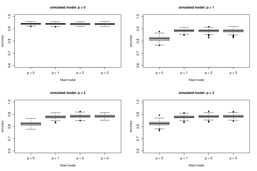
Figure 1: Boxplots of global decoding accuracies using the Viterbi algorithm for increased overlap in the state-dependent distributions ($\mu_{1}^{\text{step}}=25,\ \mu_{2}^{\text{step}}=35$).

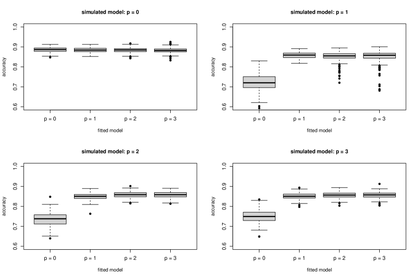
Figure 2: Boxplots of global decoding accuracies using the Viterbi algorithm for increased overlap in the state-dependent distributions ($\mu_{1}^{\text{step}}=25,\ \mu_{2}^{\text{step}}=30$).

A.3 Stability

Table 2 and Table 3 contain the proportions of global optima in the simulation with $T=250$, respective $T=500$.

Table 2: Proportion of presumably global optima when carrying out 250 iterations for each model configuration when $n=250$.

		fitted model
		$p=0$	$p=1$	$p=2$	$p=3$
simulated model	$p=0$	$1.000$	$0.960$	$0.968$	$0.972$
	$p=1$	$0.988$	$0.964$	$0.956$	$0.964$
	$p=2$	$0.972$	$0.968$	$0.952$	$0.944$
	$p=3$	$0.948$	$0.976$	$0.960$	$0.952$

Table 3: Proportion of presumably global optima when carrying out 250 iterations for each model configuration when $n=500$.

		fitted model
		$p=0$	$p=1$	$p=2$	$p=3$
simulated model	$p=0$	$1.000$	$0.976$	$0.988$	$0.992$
	$p=1$	$1.000$	$1.000$	$0.984$	$0.988$
	$p=2$	$0.996$	$0.996$	$0.972$	$0.988$
	$p=3$	$0.996$	$0.992$	$0.992$	$0.992$

A.4 Choice of complexity penalty

Figure 3 shows the development of AIC and BIC for increasing complexity penalty $\lambda\in[0,100]$ for a fixed simulated data set with true within-state autocorrelation of degree two. The fitted models allow for a maximum autoregressive degree of five in each variable and state. The vertical line indicates the optimal value of $\lambda$ regarding AIC and BIC.

Figure 4 visualizes the distribution of optimal complexity penalties when selecting based on AIC, BIC, or global decoding accuracy. It is evident that the BIC chooses most conservatively.

Figure 5 illustrates the systematic overestimation of effective degrees of freedom, compared to the true number of parameters in the underlying data-generating process. Again, the BIC reveals lower values than the other criteria, indicating it to be most suitable for model selection in our approach.

Figure 6 reveals the overall development of global decoding accuracies when increasing $\lambda$ for 100 different simulated data sets. While the accuracies remain fairly stable for low penalties, they decrease substantially if the penalties get large enough to delete autoregressive components from the model that are included in the true model formulation.

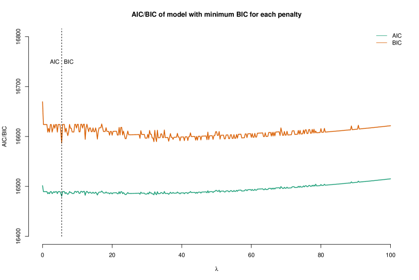
Figure 3: AIC and BIC of default simulation setting when varying $\lambda$, allowing a maximum autoregression degree of five.

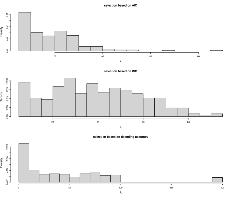
Figure 4: Histograms of chosen optimal complexity penalty $\lambda$ based on AIC, BIC and global decoding accuracy. 250 iterations on a grid of 24 values for $\lambda$ were computed in total.

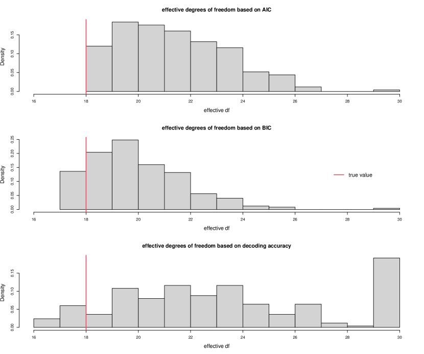
Figure 5: Histograms of effective degrees of freedom of models, selected based on AIC, BIC and global decoding accuracy. 250 iterations were computed in total.

Figure 6: Decoding accuracies of 100 lasso penalized models with varying complexity penalty $\lambda$.

Appendix B Additional application results

B.1 Additional parameter estimates of application to sea tern data

The estimated model parameters of the suggested model specification using manual exploration (within-state autoregression of first degree in state 1 and third degree in state 2) are:

$$\boldsymbol{\hat{\delta}} =(0.267,0.733);\quad\boldsymbol{\hat{\Gamma}}=\begin{pmatrix}0.684&0.316\\ 0.115&0.885\end{pmatrix}$$

$$\boldsymbol{\hat{\mu}}^{\text{step}} =(563.308,885.996);\quad\boldsymbol{\hat{\sigma}}^{\text{step}}=(212.256,79.926)$$

$$\boldsymbol{\hat{\mu}}^{\text{turn}} =(0.048,0.121);\quad\boldsymbol{\hat{\kappa}}^{\text{turn}}=(2.509,16.183)$$

The estimated autoregressive parameters amount to

$$\hat{\phi}_{1}^{\text{step}}=0.487;\quad\boldsymbol{\hat{\phi}}_{2}^{\text{step}}=(0.503,0.000,0.050);$$

$$\phi_{1}^{\text{turn}}=0.317;\quad\boldsymbol{\hat{\phi}}_{2}^{\text{turn}}=(0.770,0.000,0.000).$$

B.2 Model comparison

Table 4 compares different unpenalised model fits for the sea tern data using BIC. While the lasso penalisation selects the model with $\boldsymbol{p}=(1,1,1,1)$, the comparison of unpenalised models leads the the best result regarding BIC for $\boldsymbol{p}=(1,3,1,3)$.

	autoregressive degree
$\boldsymbol{p}$	(0,0,0,0)	(1,1,1,1)	(2,2,2,2)	(1,3,1,3)	(3,3,3,3)
$\boldsymbol{\ell}$	$-3668.65$	$-3307.06$	$-3242.76$	$-3181.89$	$-3175.46$
BIC	$\phantom{-}7399.51$	$\phantom{-}6701.21$	$\phantom{-}6597.49$	$\phantom{-}6475.76$	$\phantom{-}6487.76$

Table 4: Comparison of selected model performances for the sea tern data (1 Hz) according to the BIC, calculated based on unpenalised model fitting. The degree $(1,1,1,1)$ was chosen using the lasso-based approach.

B.3 Simulated movement tracks using estimated model parameters

To illustrate model adequacy, Figure 7 shows one of the original movement tracks (top) as well as simulated tracks from a basic HMM (bottom left) and the autoregressive HMM selected by the information criteria (bottom right) when applying automated lasso-based degree selection. The latter is able to produce more pronounced circles than the basic model formulation, leading to visually more realistic synthetic movement tracks.

Figure 7: Comparison of real data (top) to data simulated from a fitted basic HMM (bottom left) and a fitted autoregressive HMM (bottom right). In the latter case, the choice of $\lambda\approx 5.3$ corresponds to the best-scoring model based on information criteria.