Efficient Bayesian inversion for simultaneous estimation of geometry and spatial field using the Karhunen-Loève expansion
Abstract
Detection of abrupt spatial changes in physical properties representing unique geometric features such as buried objects, cavities, and fractures is an important problem in geophysics and many engineering disciplines. In this context, simultaneous spatial field and geometry estimation methods that explicitly parameterize the background spatial field and the geometry of the embedded anomalies are of great interest. This paper introduces an advanced inversion procedure for simultaneous estimation using the domain independence property of the Karhunen-Loève (K-L) expansion. Previous methods pursuing this strategy face significant computational challenges. The associated integral eigenvalue problem (IEVP) needs to be solved repeatedly on evolving domains, and the shape derivatives in gradient-based algorithms require costly computations of the Moore-Penrose inverse. Leveraging the domain independence property of the K-L expansion, the proposed method avoids both of these bottlenecks, and the IEVP is solved only once on a fixed bounding domain. Comparative studies demonstrate that our approach yields two orders of magnitude improvement in K-L expansion gradient computation time. Inversion studies on one-dimensional and two-dimensional seepage flow problems highlight the benefits of incorporating geometry parameters along with spatial field parameters. The proposed method captures abrupt changes in hydraulic conductivity with a lower number of parameters and provides accurate estimates of boundary and spatial-field uncertainties, outperforming spatial-field-only estimation methods.
keywords:
Inverse problems , Uncertainty quantification , Interface detection , Random fields , Karhunen–Loève expansion , Hamiltonian Monte Carlo , Integral eigenvalue problem[1]organization=Graduate School of Agriculture, Kyoto University, addressline=Kitashirakawa-oiwakecho, city=Sakyo-ku, postcode=606-8502 Kyoto, country=Japan \affiliation[2]organization=Engineering Risk Analysis Group, Technische Universität München, addressline=Arcisstr. 21, postcode=80290 München, country=Germany
1 Introduction
In nondestructive testing procedures, measurements are often used to estimate spatial distributions of physical properties such as hydraulic conductivity [1, 2, 3], elastic modulus [4, 5], or P- and S-wave velocities [4, 6, 7] through the solution of inverse problems. Quite often, along with the general spatial distribution of the physical property, the interest may lie in identifying unique geometric features such as buried objects, cavities, and fractures, etc. These features manifest as anomalies (extremely high or low magnitudes) in the inferred physical properties [8, 9, 10, 11, 12] and are delineated in the post-processing stage of inversion. We focus on such inverse problems within a Bayesian framework, incorporating priors and computing uncertainties in inversion results from posterior probability distributions.
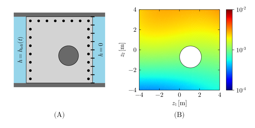
Consider the inverse problem of visualizing the interior of a target domain with unique geometric features using steady seepage flow observation data. Traditional methods do not account for geometric information, focusing solely on the spatial distribution of hydraulic conductivity. However, in practical problems, it is often possible to parametrize the geometries of these features and incorporate a set of geometry parameters into the inverse problem [13, 14, 15]. The general construct of such problems is explained through a specific example involving seepage flow in a domain shown in Fig. 1(A). This problem involves the determination of the hydraulic conductivity spatial field in the domain around a pipe (of unknown location and size) beneath the ground surface. This inverse problem can help track water leakage leading to subsequent soil erosion in the vicinity of the pipe [16]. Instead of determining the spatial field over the entire domain , it might be beneficial to encode a parameterization of the unknown location and size of the pipe-soil interface into the inverse problem and determine the spatial field only over the domain . Another example shown in Fig. 1(B) is a trans-dimensional subsurface planarly-layered stratification problem [17, 18] where along with the layer properties in each domain , , geometry parameters defining the planar layer boundaries , can also be determined during inversion. This approach, referred to as the simultaneous estimation method, contrasts with spatial-field-only estimation methods that neglect explicit geometry parameters.
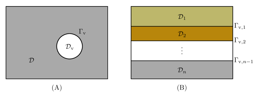
Incorporating geometry parameters allows for accurate boundary condition enforcement. For instance, in Fig. 1(A) the no-flow boundary conditions representative of actual hydraulic conditions on can be implemented easily in numerical schemes such as the finite element method. This can be done through finite element meshes that conform to the computational domain that is continuously updated as is updated during inversion. The challenge in such a shape-tracking approach is maintaining decent mesh quality during successive updates. Drawing on a method developed by Koch et al. (2020) [19], we achieve this by updating the domain from a fixed reference configuration using a mesh-moving finite element method [20]. Computation of gradients of the posterior density w.r.t the geometry parameters follows from shape sensitivity analysis [21].
Detection of sharp interfaces in material properties has historically been solved through level set methods [22, 23, 24] with great success. These methods work on a fixed domain and do not implement boundary conditions (BCs) at the interfaces. However, it must be mentioned that a conformal meshing strategy can easily be applied once the boundary has been defined by the zero contours of a level set following which BCs can be applied. For simplicity and practical utility in problems such as that in Fig. 1(A), we restrict ourselves to working with a direct parameterization of the geometry of the boundary. However, the topics discussed in subsequent sections should, in principle, be equally applicable to problems with level-set parameterizations. The explicit consideration of boundaries through these methods can aid the inversion process in detecting sharp interfaces between material domains of vastly varying (or discontinuous) physical properties—a task that is difficult to achieve, especially when the regularization scheme implemented only permits smooth solutions. This is the case in conventional Bayesian inversion techniques where Gaussian random fields with smooth autocovariance functions [25] are used as priors. In this study, we only consider stationary, isotropic autocovariance functions with a single length scale and note that approaches considering non-stationary autocovariance functions in a hierarchical setting [26] are strong alternative approaches to detect interfaces between discontinuous materials.
Our study estimates geometry and spatial field parameters simultaneously, characterizing material properties over the domain as a spatial random field and finding its posterior statistics along with those of the geometry parameters defining the boundary . This is in contrast to studies that aim to determine constant spatial properties once the boundary of an embedded object has been determined through level sets [27] or studies that treat background spatial field parameters as ‘nuisance’ parameters [13, 28]. The prior spatial random field is discretized through the Karhunen-Loève (K-L) expansion [29, 30], which is the optimal orthogonal series representation in the mean-square sense. The eigenvalues and eigenfunctions employed in the expansion are computed by solving an integral eigenvalue problem (IEVP) related to the autocovariance function of the random field defined over [31]. In practice, the K-L expansion is applied as a truncated series, and the effect of the choice of prior parameters (correlation lengths, number of terms in the truncated expansion, etc.) on the statistics of the posterior has been studied extensively in the literature [32].
In this study, the sampling of the posterior distribution over the random coefficients of the K-L expansion and the geometry parameters (Koch et al. (2021) [33]) is done through the Hamiltonian Monte Carlo (HMC) algorithm [34]. The proposals in this Markov Chain Monte Carlo (MCMC) [35, 36, 37] algorithm utilize gradient information of the target distribution and can be tuned [38, 39] to draw nearly independent samples from the posterior. This is especially useful in computationally expensive PDE-constrained inverse problems where random walks must be avoided. To satisfy the reversibility condition [40] of MCMC, a non-trivial task for simultaneous spatial field and geometry updates, we employ mesh-moving updates [19] of the finite element mesh from a fixed reference configuration. Finally, updating the boundary requires redefining the autocovariance function and computing the IEVP over the updated domain , leading to a high computational cost as the eigenpair related to the IEVP needs to be recomputed. This problem is exacerbated in HMC, where the gradients of the posterior density require a computation of the gradients of the eigenpair from the IEVP w.r.t the geometry parameters [33]. This is particularly demanding because the evaluation of the shape derivatives requires the computation of the inverse of a rank-deficient matrix related to the eigenvalue problem, thereby necessitating the computation of pseudo-inverses (e.g. Moore-Penrose inverse [41]).
In this study, we revisit the simultaneous estimation method of Koch et al. (2021) [33] with the aim of improving computational efficiency. Leveraging the domain independence property of the K-L expansion [42], which states that the first and second-order moments of a random field generated by the K-L expansion are invariant to a change in the physical domain, this study aims to:
-
1.
Develop a Bayesian inversion procedure for simultaneous spatial field and geometry inversion using conformal meshes. This includes the development of a novel gradient computation procedure.
-
2.
Investigate the difference in inversion results and computation time between the simultaneous estimation method of Koch et al. (2021) [33] and the method developed in this study.
-
3.
Highlight the advantage of explicitly considering a parameterization of the geometry in posterior statistics as compared to general spatial-field-only estimation methods.
The subsequent sections of this study are structured as follows. Section 2 explains the parameterization of the targets to be estimated, including the K-L expansion and its domain independence property. In Section 3, the forward and observation models are first described. Following this, the framework for Bayesian inference including HMC, is explained. Section 4 explains the gradient computation procedure. In Section 5, numerical analysis results of inverse analysis for one-dimensional and two-dimensional seepage flow problems are presented.
2 Modelling of the spatial random field and geometry
2.1 Karhunen-Loève expansion
Let be a probability space where is the sample space, is the algebra over , and is a probability measure on . Also, let be a bounded domain. Consider a real-valued, second-order spatial random field with a continuous mean and a continuous autocovariance function . The autocovariance function is a positive-semidefinite function which, according to Mercer’s theorem, has the spectral decomposition [30]:
| (1) |
where and are eigenvalues and eigenfunctions of the Hilbert-Schmidt integral operator corresponding to , and the eigenfunctions are orthogonal, that is, . The eigenpairs are computed as solutions to the following integral eigenvalue problem (IEVP), which is a homogeneous Fredholm integral equation of the second kind [43]:
| (2) |
With these results, it can be shown that the second-order random field can be represented through the K-L expansion as follows:
| (3) |
where are random coefficients that have the following properties: satisfies . The work in this paper applies the K-L expansion to Gaussian random fields . In this case, since the random variables are linear functions of the Gaussian field, they are independent standard normal random variables. In Eq. 3, is the complete K-L expansion of and is defined to distinguish it from the truncated K-L expansion . If are sorted in descending order, (), the truncated K-L expansion of is represented as
| (4) |
where is the number of terms considered in the expansion and should be appropriately chosen according to the covariance structure of the random field. This finite series representation of the random process is optimal in the sense of minimizing the mean-square error [30]. In Bayesian inversion, inference over the spatial random field , discretized in terms of the truncated K-L expansion, is then equivalent to inference over the apriori standard multivariate Gaussian random variable .
2.2 Domain independence property
Let be a domain bounding (i.e., ) and be a real-valued and second-order random process with the same mean and covariance function as . Also, let denote the K-L expansion of , that is,
| (5) |
where and are eigenvalues and eigenfunctions of IEVP Eq. 2 on . Since the autocovariance function corresponding to locations common to two domains, i.e., , is the same, Mercer’s theorem can be represented as
| (6) |
Then from Eqs. 3, 5 and 6, for the two K-L expansions and , the following equations hold for all :
| (7) | ||||
| (8) | ||||
| (9) |
This is called the domain independence property [42] of the K-L expansion, which states that the first and second-order moments of two random fields, generated on two overlapping domains and by K-L expansions, are the same on . In other words, even though the individual K-L terms might differ, the first and second-order moments of the random fields (or the Gaussian random field itself) generated by the K-L expansions are invariant to a change in the physical domain. Note that the domain independence property holds for the complete K-L expansion, and an error [42] is introduced when the truncated K-L expansions and are used. The behavior of this error for both the K-L expansions has been studied extensively [44]. Numerical tests on several examples have shown that the truncation error is larger for the K-L expansion of the random field defined on the bounding domain. This implies that the K-L expansion loses its optimality for representing the random field on when the K-L expansion is performed on .
2.3 Parameterization
Let be a Gaussian random field, representing a spatially varying physical property, with a known mean and autocovariance function. Then, according to the K-L expansion in Eq. 4, this Gaussian random field is implicitly represented through the parameter vector and endowed with a Gaussian prior density . Additionally, let be the parameters chosen to define the geometric features of interest. The choice of parameters depends on the prior information available about the complexity of features in question. This can include direct definitions of simple shapes [19] or more flexible parameterizations controlling the degree of continuity, slope, and curvature of the boundary such as B-splines [45]. The distribution of must be constrained to a physically sensible range. In this study, the multivariate truncated normal distribution is chosen as the prior of . If is the vector of all the parameters to be estimated, then in subsequent sections, in the spatial-field-only estimation method, and in the simultaneous estimation method. The inverse analysis is performed by determining the posterior distribution of the multivariate random variable .
For the simultaneous estimation method, it is easy to see that the computational domain is a function of the geometry parameters, i.e., . A naive implementation of the K-L expansion to discretize on domain configurations updated during inversion would require repeated evaluations of the IEVP in Eq. 2. Additionally, gradient-based Bayesian inversion algorithms such as HMC would require the expensive computation of a Moore-Penrose inverse to obtain the gradient w.r.t the geometry parameters (see Eq. 65 in A). The domain independence property offers an alternative strategy where it is not necessary to evaluate the IEVP and its derivatives for each realization . A proper choice of another domain , such as a bounding box (without holes), that bounds all possible realizations of as the geometry parameters are updated, has to be made. As all coordinates in also lie in , then due to the domain independence property, the K-L expansion of constructed on is equivalent to that on . The eigenpairs are obtained by solving the IEVP only once on the bounding domain at the beginning of inversion, and the eigenfunctions can then be interpolated to points of interest in . This strategy simplifies the gradient computation procedure, where the Moore-Penrose inverse is not required anymore (see Section 4), and helps achieve significant savings in computational cost.
2.4 K-L expansion based discretization of the hydraulic conductivity spatial random field
Working with seepage flow data, the target physical parameter of interest is the hydraulic conductivity random field . To enforce positivity constraints, this field is represented as a log-normal spatial random field which is considered to share the following relationship with the Gaussian Process :
| (10) |
Here is the lower bound on the hydraulic conductivity that guarantees . In this paper, prior information is encoded through the stationary Gaussian Process , where is the mean of , and is a smooth Gaussian autocovariance kernel:
| (11) |
where and are the scale and the correlation length, respectively.
An -term truncated K-L expansion is used to represent the random field , thereby enabling a reduction in dimensionality of the number of parameters to be estimated. Assume that a bounding domain can be constructed that bounds all possible realizations of , then for the same mean and autocovariance functions now defined on , using the domain independence property, the truncated K-L expansion of at all points can be approximated as
| (12) |
Here and are computed with respect to the IEVP Eq. 2 defined on the bounding domain , is a standard normal random vector, and is a new notation for , introduced to emphasize its parameterization by [46]. For completeness, considering Eq. 10 and Eq. 12, the log-normal random field can be restated as and is given as
| (13) |
The eigenvalues and eigenfunctions of the IEVP are obtained numerically by the Nyström method [31, 47]. Using a Gaussian quadrature scheme for numerical integration, Eq. 2 on can be approximated as
| (14) |
where are integration points, and are corresponding integration weights. The method proceeds by requiring that Eq. 14 is satisfied for , i.e.,
| (15) |
The system of equations in Eq. 15 can be written in a matrix form as
| (16) |
where is a symmetric positive semi-definite matrix with elements , is a diagonal matrix with elements , and is a vector whose th entry is . Left multiplying Eq. 16 by with elements , a matrix eigenvalue problem is obtained as follows:
| (17) |
where , . Since is a symmetric positive semi-definite matrix, and are satisfied. Noting that and using Eq. 14, the Nyström interpolation formula for the eigenfunction can be obtained as
| (18) |
where is the th entry of .
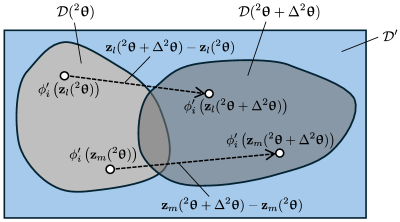
In the discussion above, it must be emphasized that , the value of the random field at the point with coordinates , depends on the geometry parameters in the simultaneous estimation method. This is because the point coordinates , at which the eigenfunctions are evaluated, move as the computational domain is updated (see Fig. 2). In this paper, the mesh updates corresponding to the computational domain, are done from a fixed reference domain to maintain reversibility of the HMC algorithm [19]. When is updated to , the value of at (i.e., ) changes to because the evaluation point moves from to . In other words, even though the shape of eigenfunctions remains fixed, the value depends on the geometry parameters . This dependence must be accounted for in the computation of gradients w.r.t the geometry parameters (see Section 4). It is worth mentioning that these gradients correspond to the advection term in the material derivative when considering as time.
3 Bayesian inference
3.1 Forward and observation models
Consider a domain that contains a soil domain (i.e., ). The steady seepage flow (ignoring transient effects) through , governed by Darcy’s law and the continuity equation, is written as
| (19) |
| (20) |
where , is the total hydraulic head, is the seepage flow velocity, is the source term, and is the hydraulic conductivity. The boundaries are classified as Dirichlet boundary or Neumann boundary (i.e., , ), with the boundary conditions given as
| (21) |
| (22) |
The term is a known hydraulic head, is the outward unit vector normal to and is the known flux on .
Consider a finite element discretization of the domain containing nodes. Taking into account that nodes are moved to conform to updated domains during inversion, the nodal coordinates matrix can be represented as . Therefore, the discretized form of Eq. 19 and Eq. 20 at depends not only on but also on and is given as
| (23) |
where are the global discretized hydraulic head and nodal flux vectors, and is the global hydraulic conductivity matrix. The elemental hydraulic conductivity matrix is
| (24) |
where is the hydraulic conductivity in the element with the central coordinates , is a matrix containing derivatives of the elemental shape functions, is the determinant of the elemental Jacobian matrix, and is the region occupied by the element in isoparametric space. Note that the dependence of and on arises from their construction using the nodal coordinates matrix for the element , which is a submatrix of .
Observations used in the inverse analysis consist of measurements of hydraulic head and flux values measured at discrete locations in . Let be the state vector, and be observations masked by Gaussian noise , where is the covariance matrix. Then, the linear measurement model is given as
| (25) |
where is the measurement model matrix. In Eq. 25 the index refers to independent observation data collected under different boundary conditions.
3.2 Bayes’ theorem
The parameter to be estimated is approximated from the posterior probability distribution given as
| (26) |
where refers to , is the likelihood, and is the prior distribution. Considering Eq. 25, can be formulated as
| (27) |
Noting that is Gaussian (see Eq. 3), if the parameter is also chosen to be Gaussian, then the prior distribution over is given by the Gaussian density
| (28) |
where is the mean, and is the covariance matrix. These quantities are chosen apriori and are set according to the inversion method; in the spatial-field-only estimation method , while in the simultaneous estimation method . Substituting Eq. 27 and Eq. 28 into Eq. 26, the posterior density can be shown to be:
| (29) |
where
| (30) |
Note that constant terms of cancel out during the calculation of the acceptance probability in any MCMC algorithms, and it is sufficient to only consider -dependent terms of .
3.3 Hamiltonian Monte Carlo
The Hamiltonian Monte Carlo (HMC) algorithm is chosen to sample the posterior distribution of Eq. 29. In HMC, auxiliary momentum variables are introduced, and a joint distribution of and is defined as
| (31) |
We make a simple choice for the probability distribution of which is independent of , i.e., . Thus, can be expressed as
| (32) |
where
| (33) |
Here, is a symmetric positive-definite mass matrix. Considering Eqs. 29, 31 and 32, the joint distribution can be represented as
| (34) |
where is the Hamiltonian and defined as
| (35) |
In this context, is called the kinetic energy, and is called the potential energy. The definition of the Hamiltonian enables the generation of deterministic trajectories of through Hamiltonian dynamics. These equations are often solved numerically by the leapfrog method, which satisfies time reversibility and volume conservation properties. This method consists of the following three steps:
| (36) |
| (37) |
| (38) |
Starting with a random draw , the current th sample is updated to the th sample candidate by applying the leapfrog steps times, with step-size . Whether is accepted or rejected as the th sample is determined by the Metropolis-Hastings acceptance criteria [48]:
| (39) |
where is the Jacobian for the conversion from to , and in the leapfrog due to volume conservation. The choice of the parameters , , and in the leapfrog scheme affects the sampling efficiency of HMC. Hence, methods that automatically tune these parameters are useful. In this study, we use an adaptation procedure similar to Stan [49]. In detail, the Dual Averaging scheme [50] is used for tuning , the No-U-Turn Sampler [38] is used for tuning , and the adaptation of is done according to section 4.2.1 in [39].
4 Gradient computation
The gradient of the negative log of the posterior density w.r.t the parameter , required in the leapfrog steps, is obtained through differentiation of Eq. 30 and is given as
| (40) |
where . Eq. 40 refers to the direct differentiation method (DDM) and involves the expensive computation of the possibly large state vectors w.r.t . This cost can be reduced through the adjoint method (AM), details of which can be found in [5, 51]. While the direct computation of can be avoided if the AM method is used, the term has to be computed both in DDM and AM. These derivatives of the FEM global hydraulic conductivity matrix , where is the gradient of the elemental hydraulic conductivity matrix, can be obtained from Eq. 24. This gradient consists of two derivatives w.r.t the spatial field and the geometry parameters (i.e., and , respectively), which are given as
| (41) |
| (42) |
The elemental domains in isoparametric space map to the domains , which are updated for every momentum update in the leapfrog scheme. The derivatives and are common in shape optimization literature and calculated in the same way as [33]. For completeness, these are given as
| (43) |
| (44) |
where is the nodal coordinate matrix for element .
The gradient of the hydraulic conductivity random field (w.r.t spatial field parameters and geometry parameters ) appears in Eq. 41 and Eq. 42, respectively. The combined vector can be obtained through a direct differentiation of Eq. 13 as
| (45) |
From the discussion in Section 2.4, it is clear that depends on both and . The derivative can be obtained from a simple differentiation of Eq. 12, and its components and are
| (46) |
| (47) |
For a numerical computation of the IEVP in Eq. 2 using the Nyström method, the shape derivatives of the eigenfunctions are obtained from Eq. 18 as
| (48) |
Here is the derivative of the autocovariance function in Eq. 11. Seeing that the integration points employed in the Nyström method (see Section 2.4) are defined on and are independent of , is given as
| (49) |
where
| (50) |
When the domain independence property of the K-L expansion is not used in the simultaneous estimation method of Koch et al. (2021) [33], the derivatives of the K-L expansion require the gradient calculations associated with the IEVP in Eq. 2. Specifically, the shape derivatives of the matrix eigenvalue problem in Eq. 17, which is the discrete form of the IEVP, must be computed. This process involves the computation of the gradients of the eigenvalues and eigenfunctions w.r.t the geometry parameters, the latter of which involves the expensive Moore-Penrose inverse. The same problem arises in random field discretization through the discrete K-L expansion [33] and is discussed in A. Furthermore, a new IEVP would be set up for every update of the domain , necessitating the computation of these expensive gradients in every step of HMC. Implementation of the domain independence property of the K-L expansion obviates the need to compute the shape derivatives of the eigenvalues. Although the shape derivatives of the eigenfunctions still have to be computed, these derivatives (see Eq. 48) only involve terms already calculated in the Nyström method and the cheap computation of the derivative of the autocovariance function.
5 Numerical experiments
The inversion is carried out using three methods: the spatial-field-only estimation method [5], the simultaneous estimation method of Koch et al. (2021) [33], and the proposed simultaneous estimation method using the domain-independence property of the K-L expansion. These methods are applied to two seepage flow problems containing geometric features of interest. In the simultaneous method of Koch et al. (2021) (see A), the discretization of the random field is done through the discrete K-L expansion [52]. The first problem is a 1D vertical seepage flow problem through a 3-layered soil where the hydraulic conductivity in the three layers as well as the actual location of the layer interfaces is unknown. The second problem involves the determination of the hydraulic conductivity in a domain where a pipe of unknown size and location is known to be present. Inversion is performed using HMC, and the program for all three methods is written in Julia based on the AdvancedHMC.jl [53] package. The impact of the prior correlation length on inversion results is examined in the following sections. Furthermore, comments are made on the computation savings achieved through the implementation of the domain independence property.
5.1 1D seepage flow problem
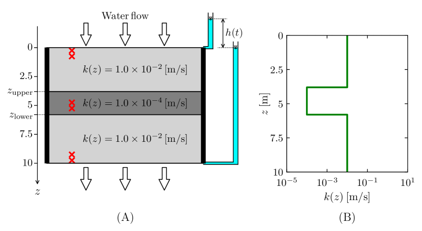
A schematic of the 1D steady vertical seepage flow through three horizontal soil layers is shown in Fig. 3(A). The target for estimation is the hydraulic conductivity spatial field in a domain , consisting of a thin clay seam in with hydraulic conductivity two orders of magnitude lower than that in the homogeneous sandy layers in the domain surrounding it. The true hydraulic conductivity field is shown in Fig. 3(B). In addition to the hydraulic conductivity field, the locations of the top and bottom boundaries of the clay seam are unknown. Dirichlet boundary conditions (BCs) are implemented such that the hydraulic head at the ground surface varies as for , while is kept fixed. Observation data consists of the hydraulic head measured at 6 points (red cross marks in Fig. 3(A)) and the water inflow rate measured at the top for 31 sets of BCs. These observations were obtained by adding Gaussian noise (mean is 0, standard deviation is 10% of the true value) to the true values. The true values are obtained numerically by solving the forward problem for the true condition on a mesh with 200 equally spaced finite elements in .
5.1.1 Comparison of estimated results
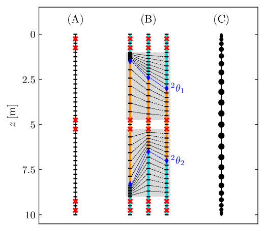
In all three methods of inversion, the log-normal hydraulic conductivity random field is spatially discretized as for 40 finite elements on (see Fig. 4(A)). Here, is the random hydraulic conductivity in the element with the central coordinate . In the spatial-field-only estimation method, is represented through the K-L expansion of the Gaussian random field with the mean according to Eq. 10. The K-L expansion is truncated at terms such that (see Eq. 4); thus, is represented by the lower-dimensional vector , leading to the Gaussian prior . The lower bound on is set to . The prior scale of the Gaussian kernel is set as , and three sets of prior correlation lengths are chosen for inversion.
In the simultaneous estimation methods, the hydraulic conductivity field is estimated separately on and (see Fig. 4(B)), defined as
| (51) |
where the domain boundaries are parameterized through . The mesh consists of 41 nodes (see Fig. 4(B)), the position of each defined through the geometry parameters as
| (52) |
The map presented in Eq. 52 identifies a unique mesh configuration for each realization of (see Fig. 4(B)). This unique mapping guarantees reversibility as the finite element global hydraulic conductivity matrix is constant for a particular realization of . Hence, updates from a reference configuration [19] are not required in this simple example, and updates can be made from the previous HMC step. Non-physical mesh realizations of the mesh are restricted through the constraints and . Additionally, the observation nodes remain fixed in space.
For the separate domains and , the hydraulic conductivity random field is divided into two parts:
| (53) |
Correspondingly, the hydraulic conductivity random vector is also divided into two vectors:
| (54) |
Here, the random vectors and are parameterized by the lower-dimensional random vectors and , respectively, through the K-L expansions. In summary, the target parameter vector components are and . The prior of is , and the prior of is set as a normal distribution truncated between the constraints mentioned above. The parameters , , , and the condition to determine the number of K-L expansion terms ( and ) are the same as in the spatial-field-only case. The prior correlation lengths chosen for inversion are . Here, it is expected that larger correlation lengths (relative to the spatial-field-only estimation case) should be sufficient to characterize the homogeneous spatial random fields as the geometry parameters represent the abrupt spatial changes in hydraulic conductivity. In the proposed method, the bounding domain is defined as , where the IEVP is solved with integration points (see Fig. 4(C)) using the Nyström method.
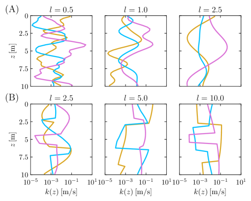
Realizations from the prior for different correlation lengths in the spatial-field-only estimation case and the simultaneous estimation case are shown in Fig. 5(A) and Fig. 5(B), respectively. In Fig. 5(A), the smaller is, the higher the frequency of spatial change of realizations, which indicates that a sufficiently small correlation length is necessary to capture rapid changes. However, sharp jumps cannot be achieved with such smooth priors. Incorporation of apriori information about the presence of a thin clay seam sandwiched between sandy layers, through geometry parameters, enables sampling of hydraulic conductivity profiles (see Fig. 5(B)) that display spatial jumps.
Five Markov chains are generated from different starting points sampled from the prior distribution, each containing 25000 samples. Automatic parameter tuning of the leapfrog parameters and , and the mass matrix (in a manner similar to Stan’s HMC adaptation [49]) is done during the first 5000 iterations, consisting of the burn-in period. The initial step-size is set to , and the mass matrix is chosen as the inverse of the covariance matrix of the prior of , i.e., (see Eq. 28).
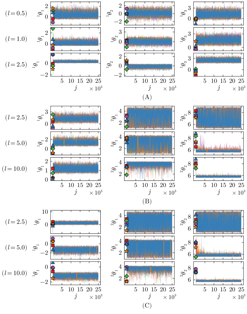
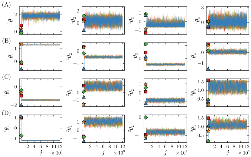
Samples from the burn-in period are discarded during posterior inference. Trace plots of the Markov chains are shown in Fig. 6, indicating all the chains with different starting points converge in the same range. Convergence of Markov chains is also confirmed by the multivariate effective sample size () [54, 55, 56]. The Markov chain is considered convergent when the consistent estimator of , which is obtained from the generated samples, is above a threshold value (called minimum ESS) as follows:
| (55) |
where the RHS is the minimum ESS, is the desired level of precision for the volume of asymptotic confidence interval, is the quantile of the chi-squared distribution , and is the gamma function. Table 1 shows (the dimension of ), the mESS, and the minimum ESS for each analysis. All mESS values are larger than each minimum ESS, indicating that the samples are well converged to the target distributions. Here, it must be noted that, because the simultaneous estimation case allows for the use of relatively larger correlation lengths, the dimensionality of the inverse problem (see Table 1) can be reduced in comparison to the spatial-field-only case. This points to the fact that the introduction of geometry parameters does not complicate the analysis, but rather simplifies it and helps alleviate the curse of dimensionality.
| minESS | mESS | |||
|---|---|---|---|---|
| Spatial-field-only [5] | 0.5 | 28 | 8592 | 26906.66 |
| 1.0 | 15 | 8793 | 29189.73 | |
| 2.5 | 8 | 8804 | 38391.09 | |
| Simultaneous [33] | 2.5 | 13 | 8817 | 16918.24 |
| 5.0 | 10 | 8831 | 10135.66 | |
| 10.0 | 9 | 8823 | 21057.63 | |
| Simultaneous (proposed) | 2.5 | 16 | 8778 | 38176.65 |
| 5.0 | 12 | 8826 | 12946.18 | |
| 10.0 | 8 | 8804 | 15959.50 |
Results from the spatial-field-only estimation method for three different prior correlation lengths are shown in Fig. 7(A). In the case of , the hydraulic conductivity tends to be small in the central part of the domain. However, the 95% CI does not envelop the true spatial field. This is because is large relative to the width of the central part of the domain with different hydraulic conductivity, and the K-L expansion is unable to resolve abrupt spatial changes in hydraulic conductivity. In the case of , the 95% CI is larger than in the case of , but it fails to envelop the true spatial field and also does not capture the spatial change in hydraulic conductivity. In the case of , the 95% CI envelops most of the true spatial field. However, this result is not sufficiently accurate, as there is a large variance around both ends of the domain.
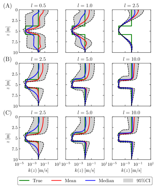
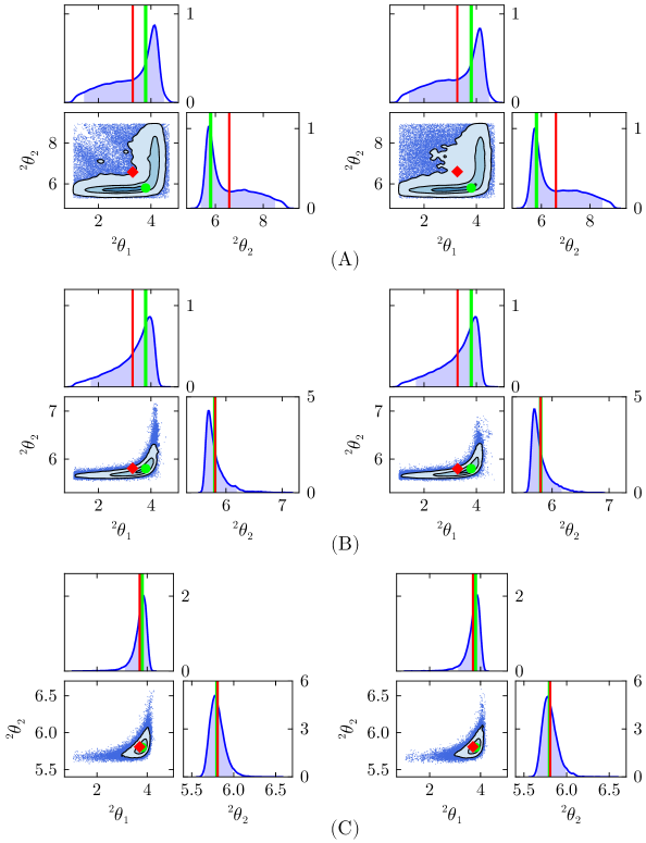
The estimated hydraulic conductivity spatial field using the simultaneous estimation method of Koch et al. (2021) [33] and the proposed simultaneous estimation method are shown in Fig. 7(B) and Fig. 7(C), respectively. The results of both methods are almost identical. In other words, the proposed method does not compromise the performance of the simultaneous estimation of Koch et al. (2021) [33], and the small error due to the truncation of the K-L expansion associated with the domain independence property (see Section 2.2) has a negligible effect on the inversion results. For all correlation lengths, the 95% CIs envelop most of the true spatial fields. In particular, in the case of , the incorporation of geometry parameters clearly enables HMC to resolve jumps in the spatial field, as seen in the posterior mean, median, and narrow 95% CI. However, the width of the 95% CIs increases, and the resolution of the jump decreases as the prior correlation length decreases. This difference due to the correlation length can be explained as follows. Spatial field realizations with smaller correlation lengths display a higher frequency of spatial oscillation (see Fig. 5(B)) in and around the true (constant) hydraulic conductivity field. Among these realizations, there can be many spatial fields, which while differing from the true spatial conductivity field, generate a forward response such that the error from the observation data is nearly identical. This results in a situation where the posterior has a large variance and is influenced by the prior relatively more than by the likelihood. This trend can also be seen in the posterior distributions of in Fig. 8. The effect of the prior in the posterior is more significant at smaller correlation lengths, as seen in Fig. 8(A), wherein a larger number of samples are skewed towards the normal prior truncated between constraints mentioned earlier in this section. This behavior leads to a larger variance and an inability to differentiate between geometry parameters in the posterior, and the mean and median of the hydraulic conductivity spatial field appear similar to the case in which geometry parameters are not considered. Consequently, these results highlight the importance of an appropriate choice of correlation length parameters in the inverse analysis.
5.1.2 Comparison of computation times for the two simultaneous estimation methods
In this section, the computation time for the derivative of the K-L expansion and one leapfrog step are measured for the two simultaneous estimation methods. To be precise, the total computation time for and , which accounts for the majority of the leapfrog computation time, is measured and considered as the computation time of one leapfrog step. The number of terms in the K-L expansion is for both cases, and the correlation length is . Different meshes with 40, 120, 240, 400, 640, 1000, 1600, 2520, 4000, 6400, and 10000 finite elements are considered, and is set to and as representative values. The parameters , , the BCs, the constraints of , the prior of , and the observation data are the same as in Section 5.1.1. The HMC parameters and are set to the same initial values as in Section 5.1.1.
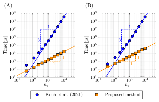
The computational time of the derivative of the K-L expansion for the two estimation methods is shown in Fig. 9(A). The slope for the method of Koch et al. (2021) [33] asymptotically approaches 3, demonstrating that the time complexity is . This result is due to the Moore-Penrose inverse, whose time complexity is , which is derived from the singular value decomposition [57]. On the other hand, the slope for the proposed method is approximately 1, indicating that the time complexity order is . This is because the derivative of the eigenfunction, which has time complexity independent of (see Eq. 48), is computed for positions. Therefore, the time complexity can be improved by approximately two orders of magnitude through the use of the domain independence property, which avoids the computation of the Moore-Penrose inverse.
Fig. 9(B) shows the computation time for one leapfrog step, which includes the cost of the finite element forward solver. The slope of the line for the method of Koch et al. (2021) [33] is almost the same as in Fig. 9(A), indicating that the main source of the computational cost in the simultaneous method of Koch et al. (2021) [33] is the derivative of the K-L expansion. On the other hand, the line for the proposed method is shifted up compared to Fig. 9(A) but retains a slope of 1. This implies that the computation time of the derivative of the K-L expansion is not dominant in the entire analysis. The unit slope refers to an time complexity, which is to be expected. This is because the computational cost of the forward analysis is also since the global matrix in this 1D seepage problem is symmetric and tridiagonal. In more general cases in 2D and 3D, the time complexity of forward analysis, using FEM, ranges from to , where the exact time complexity depends on the linear solver and the sparsity of the global matrix [57, 58]. Therefore, in the simultaneous method of Koch et al. (2021) [33], the computation of the derivative of the K-L expansion is the primary source of the computational cost. In contrast, this computation is avoided and is no longer a bottleneck in the proposed method.
5.2 2D seepage flow problem
The second inverse problem shown in Fig. 10 is related to 2D seepage flow. The target domain has a circular cavity with an impermeable boundary. The true center coordinates and radius of the circular cavity are , which are considered unknown in the inverse problem. The true spatial field of hydraulic conductivity is generated numerically through expressed by the K-L expansion with parameters , and is shown in Fig. 10(B). Dirichlet BCs are implemented such that the hydraulic head on the left end varies as for , while the hydraulic head on the right end is fixed as . Zero water flux Neumann BCs are implemented on the top and bottom sides of the domain and on the circular cavity boundary. Observation data consists of hydraulic heads at 22 points (black circles in Fig. 10(A)) and outflow discharge rate from 8 sections (divided by black horizontal bars in Fig. 10(A)). The data is generated numerically by adding zero mean Gaussian noise with standard deviation (10% of the true value) to the true values, obtained by solving the forward problem using FEM.
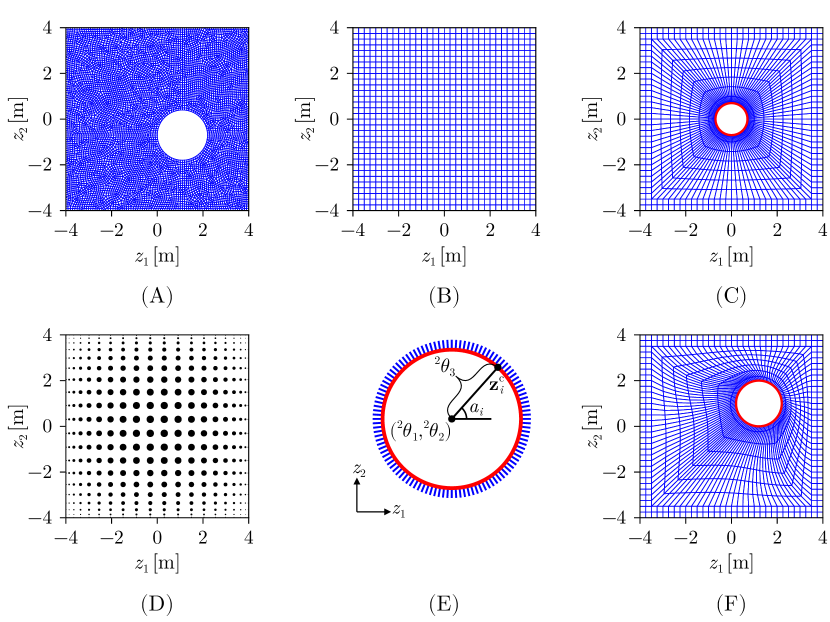
The spatial-field-only estimation does not assume the presence of the water-impermeable zone inside the target domain and is performed on a uniform structured mesh with elements of size 0.25 m, which is coarser than the observed mesh (see Fig. 11(A)). The target to be estimated is the 1024-dimensional hydraulic conductivity random vector , whose entries correspond to 1024 finite elements in Fig. 11(B). The random vector is derived from the -term truncated K-L expansion of with the mean , and its prior is . The criterion for selecting is , where is the maximum eigenvalue, and the lower bound of is set . The scale of the autocovariance matrix is set to , and two prior correlation lengths, i.e., , are chosen to study the inversion results.
Simultaneous spatial field and geometry estimation is performed only by the proposed method. This estimation assumes the presence of the water-impermeable zone inside the target domain. Therefore, the targets to be estimated are the geometry parameter vector and the 1024-dimensional hydraulic conductivity random vector , whose entries correspond to 1024 finite elements in Fig. 11(C). The random vector is derived from the -term truncated K-L expansion of . The eigenvalues and eigenfunctions in the K-L expansion are obtained by solving the IEVP on the bounding domain defined as }. The grid of Gauss quadrature points for numerical integration of the IEVP are shown in Fig. 11(D). The parameters , , , and the condition to determine are set identically to those in the spatial-field-only estimation case. Inversion is performed considering two correlation lengths, i.e., . Additionally, through the introduction of geometry parameters, it is possible to accurately implement the impermeable boundary conditions on the circular cavity boundary.
The mesh in Fig. 11(C) moves each time is updated according to the reversible mesh moving method detailed in Koch et al. (2020) [19]. This method implements mesh movement by elastically deforming a fixed reference mesh, which is the starting point of the deformation, through prescribed displacements. Since all deformation takes place through the reference mesh, the deformation is guaranteed to be reversible. Updates in define the new position of the cavity boundary, thereby yielding the prescribed displacements of the cavity boundary nodes. In this analysis, the updated position of the 112 nodes describing the boundary of the circular cavity is given as
| (56) |
where refers to the coordinates of th node on the circle, is the angle corresponding to th node as shown in Fig. 11(E). During this mesh moving phase, the BC is set to zero displacement on the outer boundaries of the domain, and the observation points are kept fixed. A decent mesh quality (see Fig. 11(F)) is maintained by considering an artificial elastic modulus that is scaled by the determinant of the element Jacobian. The elemental stiffness matrix on the reference mesh is written as
| (57) |
where is Jacobian, is a strain-displacement matrix, is the constitutive matrix, is stiffening power, and is an arbitrary scaling parameter. For all elements, the Young’s modulus and Poisson’s ratio, which determine , are set at 2500 MPa and 0.25, respectively, while both parameters and are set to 1. The prior of is a truncated Gaussian defined through the Gaussian density and the constraints:
| (58) |
to avoid mesh breakage and non-physical realizations of the circular cavity.
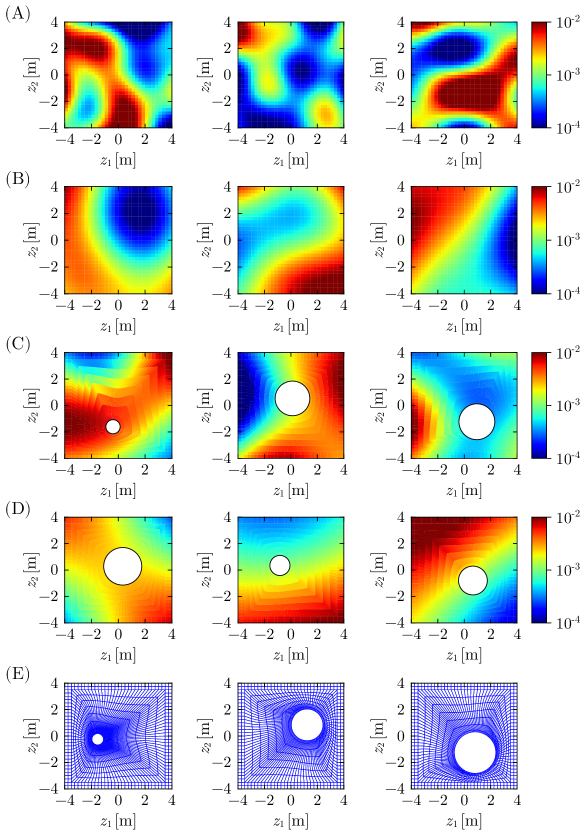
Realizations from the prior for the two estimation approaches are shown in Fig. 12. In the spatial-field-only estimation method, as in the 1D case, it is obvious that small correlation lengths are necessary to capture rapidly oscillating spatial fields. Additionally, it is clear from Fig. 12(A) and Fig. 12(B), that the spatial change of the hydraulic conductivity field is gradual, suggesting that even if the rough location of the water-impermeable circle is detected, the location of its interface would not be estimated clearly. In contrast, in Fig. 12(C) and Fig. 12(D), the realizations include holes due to the introduction of geometry parameters. This explicitly provides interface locations in the simultaneous estimation results. For completeness, Fig. 12(E) shows meshes corresponding to realizations from the prior of geometry parameters in the simultaneous estimation method.
Four chains, each containing 12,000 samples, are obtained using HMC, starting from points randomly drawn from the prior distribution. Similar to the 1D analysis, automatic parameter tuning of the leapfrog parameters , and the mass matrix is done during the first 2000 iterations. Samples from this burn-in period are discarded during posterior inference.
As in the 1D case, the Markov chain convergence is confirmed by trace plots and the mESS. In all trace plots (see Fig. 13), the chains originating from different starting points converge in the same range, and each chain converges to its high probability region quickly. In Table 2, all mESS values are larger than each minimum ESS. Based on these two criteria, we judge the Markov chains to be converged. Once again, fewer terms are required in the simultaneous estimation case, as the discontinuities in the spatial field are captured by geometry parameters explicitly.
| minESS | mESS | |||
|---|---|---|---|---|
| Spatial-field-only [5] | 2 | 28 | 8592 | 26036.70 |
| 4 | 11 | 8831 | 10535.25 | |
| Simultaneous (proposed) | 4 | 14 | 8806 | 10398.88 |
| 8 | 9 | 8823 | 11851.81 |
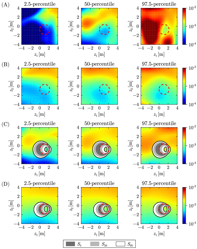
The results of the spatial-field-only estimation are shown in Fig. 14(A) and Fig. 14(B) with the 2.5, 50, and 97.5 percentiles of the hydraulic conductivity. In the case of , the estimated spatial field is similar to the true one in that the hydraulic conductivity tends to be higher at the top and lower at the bottom. The zone with relatively low hydraulic conductivity in the lower right quadrant of the domain reflects the presence of an impermeable area. However, this low hydraulic conductivity zone deviates from the true position of the circle (corresponding to the red circle in Fig. 14). Additionally, it is almost impossible to demarcate the boundary of this impermeable zone. In the case of , the 50-percentile result has a similar hydraulic conductivity trend to the true field, varying from larger values at the top to lower values at the bottom of the domain. However, the 2.5-percentile and the 97.5-percentile, the boundaries of 95% CI, have more than 2 orders of magnitude differences. The large variance in the estimation results makes it difficult to draw useful conclusions of the uncertainty in the location of the impermeable circular cavity and the surrounding hydraulic conductivity spatial field.
The results of the proposed simultaneous estimation method are shown in Fig. 14(C) and Fig. 14(D). The heatmap of the hydraulic conductivity spatial field is overlain with a contour plot reflecting the location of the impermeable boundary of the circular cavity. In both cases of and , the estimated spatial fields are similar to the true field. The 95% CIs are not large and envelope the true fields in most locations, indicating the high accuracy of the estimation results with respect to the spatial field. The grey-scale contour plot has three zones with different color depths and two black contours. Darker colors represent a higher probability that an interface is present, and the zone bounded by the two black contours corresponds to the 95% HPD (High Probability Density) of . In more detail, we define as the smallest zone that completely encompasses all circle interfaces generated by samples belonging to the % HPD region. Then, the zone within the darkest color is , within the darkest and second darkest color is , and within all three zones is . Clearly, the 95% HPD region (between the two black contours) envelops the impermeable boundary of the circular cavity in both cases and . In particular, in the case of , the darkest color zone matches the true interface well, indicating a high accuracy of the estimated results.
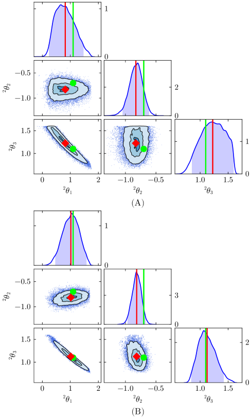
The marginal distributions of the posterior of the geometry parameters in the simultaneous estimation case are shown in Fig. 15. In the case of (Fig. 15(A)), the 95% HPDs of , , and envelop their true values, and the estimation results are sufficiently accurate. In the case of (Fig. 15(B)), which corresponds to the correlation length of the true hydraulic conductivity field, 95% HPDs for , , and envelop their true values, and these CIs are smaller than those seen in (Fig. 15(A)). Furthermore, their means are nearly identical to the true values. Additionally, in the bivariate marginal distributions, the 95% HPD regions for are narrower than those for . Overall, unlike the spatial-field-only estimation method, the proposed simultaneous estimation method provides more reliable quantification of uncertainties associated with the circular cavity boundary and the hydraulic conductivity spatial field.
6 Concluding Remarks
This paper proposes an inversion procedure for simultaneous geometry and spatial field estimation using the domain independence property of the K-L expansion. The method addresses the computational bottleneck in traditional simultaneous estimation methods caused by the repeated evaluation of the domain-dependent integral eigenvalue problem (IEVP) on evolving physical domains. By solving the IEVP once on a fixed bounding domain and using these results throughout the inversion process, the proposed method avoids repeated costly computations, significantly improving computational efficiency over previous simultaneous estimation methods [33]. In particular, the expensive computations of the Moore-Penrose inverse to obtain the shape derivatives are completely eliminated.
Performance comparisons between the proposed method and the method of Koch et al. (2021) [33] reveal substantial computational gains. Two orders of magnitude improvement in the K-L expansion gradient computation time is observed with time complexity in the proposed method established as . For the 1D seepage flow problem, the time complexity for the computation of one leapfrog step (which includes the cost of the finite element forward solver and the derivative of the K-L expansion), in the proposed method, is also observed to be . This cost is similar to that incurred in the computation of the forward solver in 1D. In general, in higher dimensions, the time complexity of the forward solver lies in a range between and , implying that the time complexity of derivative of the K-L expansion is no longer a bottleneck. Additionally, for an approximate implementation of the domain independence property with a K-L expansion truncated to terms such that , the estimation results of the proposed simultaneous estimation method are almost identical to those of the simultaneous estimation method of Koch et al. (2021) [33]. This confirms that the approximation made by using a truncated set of eigenpairs, computed on the bounding domain, in the K-L expansion is sufficient to represent the spatial random field accurately on updated domains during inversion.
Methodological advantages of the simultaneous estimation method are also demonstrated. In the inverse problem for 1D seepage flow, geometry parameters are incorporated to define the unknown interface depths of a thin clay seam sandwiched between two homogeneous sandy layers. This approach enables the capture of abrupt jumps in posterior samples of the hydraulic conductivity spatial random field. In contrast, the spatial-field-only estimation method cannot detect such jumps, regardless of the size of the correlation length. Specifically, a large correlation length produces a smooth spatial distribution, whereas a small correlation length exhibits a large variance. In simultaneous estimation, although the 95% CIs completely envelop the true hydraulic conductivity profile for all choices of correlation lengths, the width of the 95% CIs varies with correlation lengths. This reveals the importance of selecting an appropriate correlation length.
The inverse problem for 2D seepage flow is set up in a domain containing an impermeable circular cavity of unknown location and size. The incorporation of geometry parameters defining the impermeable circular boundary allows for the implementation of accurate zero-flux BCs. As in the 1D case, smooth realizations from the posterior make it difficult to infer the uncertainty in the location of the circular cavity boundary using the spatial-field-only estimation method. On the other hand, the proposed simultaneous estimation method yields accurate estimates of the hydraulic conductivity spatial field by providing straightforward estimates of the impermeable cavity boundary location and its uncertainties, thereby outperforming the spatial-field-only approach. Additionally, it is observed that the incorporation of the geometry parameters can reduce the dimensionality of the inverse problem compared to the spatial-field-only approach. This is because the spatial discontinuities are parameterized by geometry parameters apriori, and the choice of a small correlation length is unnecessary.
Based on the numerical results, it is clear that an appropriate choice of the prior correlation length parameter is essential for obtaining accurate posterior estimates. One potential future extension to this study is the inference of this parameter during the Bayesian updating process. This poses the challenge that the formulation of the IEVP changes with changes in the correlation length. In [59], a parametrized K-L expansion is proposed that could be implemented in this context. Another possible future research theme could be to combine this approach with an immersed boundary method, such as the finite cell method [60], which would avoid remeshing. Finally, HMC faces challenges in identifying multi-modal posteriors, that often appear in practical engineering problems. The proposed method could implement HMC within a sequential Monte Carlo approach that enables efficient sampling of multimodal targets.
Acknowledgements
This work was supported by JSPS KAKENHI Grant Number JP22K18352.
Appendix A Discrete Karhunen-Loève expansion and its derivative in HMC
The K-L expansion for a random vector is known as the discrete K-L expansion [61]. Let the random vector be the spatial discretization of , on a set of discrete points . In the discrete K-L expansion, the following eigenvalue problem for the covariance matrix is solved:
| (59) |
where the covariance matrix is a symmetric positive semi-definite matrix with elements , and are eigenvalues and eigenvectors of , and are orthogonal, that is, . The eigen decomposition corresponds to Mercer’s theorem for . The discrete K-L expansion is represented as
| (60) |
where , and satisfies , . The truncated discrete K-L expansion is then expressed as
| (61) |
The derivative of with respect to the K-L expansion parameters is given by
| (62) |
and the derivative of with respect to the geometry parameters is given by
| (63) |
The shape derivatives of eigenvalues and eigenvectors are analytically computed by the method of Magnus [41], and are given by
| (64) |
| (65) |
These derivatives are computed every time the parameters are updated in HMC. In particular, the calculation of requires the Moore-Penrose pseudoinverse and is the main reason for the high computational cost in a naive implementation of simultaneous spatial-field and geometry estimation.
References
- [1] D. McLaughlin, L. R. Townley, A reassessment of the groundwater inverse problem, Water Resources Research 32 (5) (1996) 1131–1161. doi:10.1029/96WR00160.
- [2] J. Lee, P. K. Kitanidis, Large-scale hydraulic tomography and joint inversion of head and tracer data using the Principal Component Geostatistical Approach (PCGA), Water Resources Research 50 (7) (2014) 5410–5427. doi:10.1002/2014WR015483.
- [3] H.-Q. Yang, L. Zhang, J. Xue, J. Zhang, X. Li, Unsaturated soil slope characterization with Karhunen–Loève and polynomial chaos via Bayesian approach, Engineering with Computers 35 (1) (2019) 337–350. doi:10.1007/s00366-018-0610-x.
- [4] S. S. Parida, K. Sett, P. Singla, An efficient PDE-constrained stochastic inverse algorithm for probabilistic geotechnical site characterization using geophysical measurements, Soil Dynamics and Earthquake Engineering 109 (2018) 132–149. doi:10.1016/j.soildyn.2018.01.030.
- [5] M. C. Koch, K. Fujisawa, A. Murakami, Adjoint Hamiltonian Monte Carlo algorithm for the estimation of elastic modulus through the inversion of elastic wave propagation data, International Journal for Numerical Methods in Engineering 121 (6) (2020) 1037–1067. doi:10.1002/nme.6256.
- [6] A. Fathi, B. Poursartip, K. H. Stokoe II, L. F. Kallivokas, Three-dimensional P- and S-wave velocity profiling of geotechnical sites using full-waveform inversion driven by field data, Soil Dynamics and Earthquake Engineering 87 (2016) 63–81. doi:10.1016/j.soildyn.2016.04.010.
- [7] K. T. Tran, M. McVay, M. Faraone, D. Horhota, Sinkhole detection using 2D full seismic waveform tomography, Geophysics 78 (5) (2013) R175–R183. doi:10.1190/geo2013-0063.1.
- [8] R. Putiška, M. Nikolaj, I. Dostál, D. Kušnirák, Determination of cavities using electrical resistivity tomography, Contributions to Geophysics and Geodesy 42 (2) (2012) 201–211. doi:10.2478/v10126-012-0018-3.
- [9] E. Cardarelli, G. Di Filippo, E. Tuccinardi, Electrical resistivity tomography to detect buried cavities in Rome: a case study, Near Surface Geophysics 4 (6) (2006) 387–392. doi:10.3997/1873-0604.2006012.
- [10] N. Adamo, N. Al-Ansari, V. Sissakian, J. Laue, S. Knutsson, Geophysical methods and their applications in dam safety monitoring, Journal of Earth Sciences and Geotechnical Engineering 11 (1) (2021) 291–345. doi:10.47260/jesge/1118.
- [11] S. Ahmed, P. J. Carpenter, Geophysical response of filled sinkholes, soil pipes and associated bedrock fractures in thinly mantled karst, east-central Illinois, Environmental Geology 44 (6) (2003) 705–716. doi:10.1007/s00254-003-0812-3.
- [12] Y. Hussain, R. Uagoda, W. Borges, J. Nunes, O. Hamza, C. Condori, K. Aslam, J. Dou, M. Cárdenas-Soto, The potential use of geophysical methods to identify cavities, sinkholes and pathways for water infiltration, Water 12 (8) (2020) 2289. doi:10.3390/w12082289.
- [13] T. Lähivaara, N. F. D. Ward, T. Huttunen, J. P. Kaipio, K. Niinimäki, Estimating pipeline location using ground-penetrating radar data in the presence of model uncertainties, Inverse Problems 30 (11) (2014) 114006. doi:10.1088/0266-5611/30/11/114006.
- [14] L. T. Nguyen, T. Nestorović, Reconstructing disturbance zones ahead of the tunnel face by elastic waveform inversion supported by a parametric level-set representation, Soil Dynamics and Earthquake Engineering 115 (2018) 606–621. doi:10.1016/j.soildyn.2018.09.025.
- [15] R. Takamatsu, K. Fujisawa, K. Nakahata, A. Murakami, Shape detection of multiple subsurface cavities by particle filtering with elastic wave propagation, International Journal for Numerical and Analytical Methods in Geomechanics 44 (15) (2020) 2025–2041. doi:10.1002/nag.3117.
- [16] M. Sato, R. Kuwano, Influence of location of subsurface structures on development of underground cavities induced by internal erosion, Soils and Foundations 55 (4) (2015) 829–840. doi:10.1016/j.sandf.2015.06.014.
- [17] A. Malinverno, Parsimonious Bayesian Markov chain Monte Carlo inversion in a nonlinear geophysical problem, Geophysical Journal International 151 (3) (2002) 675–688. doi:10.1046/j.1365-246X.2002.01847.x.
- [18] Z.-J. Cao, S. Zheng, D.-Q. Li, K.-K. Phoon, Bayesian identification of soil stratigraphy based on soil behaviour type index, Canadian Geotechnical Journal 56 (4) (2019) 570–586. doi:10.1139/cgj-2017-0714.
- [19] M. C. Koch, K. Fujisawa, A. Murakami, Novel parameter update for a gradient based MCMC method for solid-void interface detection through elastodynamic inversion, Probabilistic Engineering Mechanics 62 (2020) 103097. doi:10.1016/j.probengmech.2020.103097.
- [20] K. Stein, T. Tezduyar, R. Benney, Mesh moving techniques for fluid-structure interactions with large displacements, J. Appl. Mech. 70 (1) (2003) 58–63. doi:10.1115/1.1530635.
- [21] J. Haslinger, R. A. E. Mäkinen, Introduction to Shape Optimization: Theory, Approximation, and Computation, SIAM, Philadelphia, 2003. doi:10.1137/1.9780898718690.
- [22] A. Aghasi, M. Kilmer, E. L. Miller, Parametric level set methods for inverse problems, SIAM Journal on Imaging Sciences 4 (2) (2011) 618–650. doi:10.1137/100800208.
- [23] M. S. McMillan, C. Schwarzbach, E. Haber, D. W. Oldenburg, 3D parametric hybrid inversion of time-domain airborne electromagnetic data, Geophysics 80 (6) (2015) K25–K36. doi:10.1190/geo2015-0141.1.
- [24] M. A. Iglesias, Y. Lu, A. M. Stuart, A Bayesian level set method for geometric inverse problems, Interfaces and Free Boundaries 18 (2) (2016) 181–217. doi:10.4171/ifb/362.
- [25] C. K. Williams, C. E. Rasmussen, Gaussian Processes for Machine Learning, Vol. 2, MIT press Cambridge, MA, 2006.
- [26] D. Calvetti, E. Somersalo, Hypermodels in the Bayesian imaging framework, Inverse Problems 24 (3) (2008) 034013. doi:10.1088/0266-5611/24/3/034013.
- [27] L. Holbach, M. Gurnis, G. Stadler, A Bayesian level set method for identifying subsurface geometries and rheological properties in Stokes flow, Geophysical Journal International 235 (1) (2023) 260–272. doi:10.1093/gji/ggad220.
- [28] P. Belliveau, E. Haber, Parametric level-set inverse problems with stochastic background estimation, Inverse Problems 39 (7) (2023) 075003. doi:10.1088/1361-6420/acd413.
- [29] M. Loève, Probability Theory II, 4th Edition, Springer, New York, NY Heidelberg, 1978.
- [30] R. G. Ghanem, P. D. Spanos, Stochastic Finite Elements: A Spectral Approach, revised edition Edition, Dover Publications, Minneola, N.Y, 2012.
- [31] W. Betz, I. Papaioannou, D. Straub, Numerical methods for the discretization of random fields by means of the Karhunen–Loève expansion, Computer Methods in Applied Mechanics and Engineering 271 (2014) 109–129. doi:10.1016/j.cma.2013.12.010.
- [32] F. Uribe, I. Papaioannou, W. Betz, D. Straub, Bayesian inference of random fields represented with the Karhunen–Loève expansion, Computer Methods in Applied Mechanics and Engineering 358 (2020) 112632. doi:10.1016/j.cma.2019.112632.
- [33] M. C. Koch, M. Osugi, K. Fujisawa, A. Murakami, Hamiltonian Monte Carlo for Simultaneous Interface and Spatial Field Detection (HMCSISFD) and its application to a piping zone interface detection problem, International Journal for Numerical and Analytical Methods in Geomechanics 45 (17) (2021) 2602–2626. doi:10.1002/nag.3279.
- [34] R. M. Neal, MCMC Using Hamiltonian Dynamics, in: Handbook of Markov Chain Monte Carlo, Chapman and Hall/CRC, 2011, pp. 113–162.
- [35] N. Metropolis, A. W. Rosenbluth, M. N. Rosenbluth, A. H. Teller, E. Teller, Equation of state calculations by fast computing machines, The journal of chemical physics 21 (6) (1953) 1087–1092. doi:10.1063/1.1699114.
- [36] W. K. Hastings, Monte Carlo sampling methods using Markov chains and their applications, Biometrika (1970). doi:10.1093/biomet/57.1.97.
- [37] D. Gamerman, H. F. Lopes, Markov Chain Monte Carlo: Stochastic Simulation for Bayesian Inference, Chapman and Hall/CRC, 2006. doi:10.1201/9781482296426.
- [38] M. D. Hoffman, A. Gelman, The No-U-Turn sampler: adaptively setting path lengths in Hamiltonian Monte Carlo, Journal of Machine Learning Research 15 (47) (2014) 1593–1623.
- [39] M. Betancourt, A conceptual introduction to Hamiltonian Monte Carlo (Jul. 2018). arXiv:1701.02434, doi:10.48550/arXiv.1701.02434.
- [40] S. Chib, E. Greenberg, Understanding the Metropolis-Hastings algorithm, The american statistician 49 (4) (1995) 327–335. doi:10.1080/00031305.1995.10476177.
- [41] J. R. Magnus, On differentiating eigenvalues and eigenvectors, Econometric Theory 1 (2) (1985) 179–191. doi:10.1017/S0266466600011129.
- [42] S. Pranesh, D. Ghosh, Faster computation of the Karhunen–Loève expansion using its domain independence property, Computer Methods in Applied Mechanics and Engineering 285 (2015) 125–145. doi:10.1016/j.cma.2014.10.053.
- [43] O. Le Maître, O. M. Knio, Spectral Methods for Uncertainty Quantification: With Applications to Computational Fluid Dynamics, Springer Science & Business Media, 2010. doi:10.1007/978-90-481-3520-2.
- [44] I. Papaioannou, Non-intrusive finite element reliability analysis methods, Ph.D. thesis, Technische Universität München (2012).
- [45] G. Bugeda, J. Oliver, A general methodology for structural shape optimization problems using automatic adaptive remeshing, International Journal for Numerical Methods in Engineering 36 (18) (1993) 3161–3185. doi:10.1002/nme.1620361807.
- [46] Y. M. Marzouk, H. N. Najm, Dimensionality reduction and polynomial chaos acceleration of Bayesian inference in inverse problems, Journal of Computational Physics 228 (6) (2009) 1862–1902. doi:10.1016/j.jcp.2008.11.024.
- [47] W. H. Press, Numerical Recipes 3rd Edition: The Art of Scientific Computing, Cambridge university press, 2007.
- [48] H. M. Afshar, R. Oliveira, S. Cripps, Non-volume preserving Hamiltonian Monte Carlo and No-U-TurnSamplers, in: Proceedings of The 24th International Conference on Artificial Intelligence and Statistics, PMLR, 2021, pp. 1675–1683.
- [49] B. Carpenter, A. Gelman, M. D. Hoffman, D. Lee, B. Goodrich, M. Betancourt, M. Brubaker, J. Guo, P. Li, A. Riddell, Stan: A probabilistic programming language, Journal of Statistical Software 76 (2017) 1–32. doi:10.18637/jss.v076.i01.
- [50] Y. Nesterov, Primal-dual subgradient methods for convex problems, Mathematical Programming 120 (1) (2009) 221–259. doi:10.1007/s10107-007-0149-x.
- [51] R.-E. Plessix, A review of the adjoint-state method for computing the gradient of a functional with geophysical applications, Geophysical Journal International 167 (2) (2006) 495–503. doi:10.1111/j.1365-246X.2006.02978.x.
- [52] W. Li, O. A. Cirpka, Efficient geostatistical inverse methods for structured and unstructured grids, Water resources research 42 (6) (2006). doi:10.1029/2005WR004668.
- [53] K. Xu, H. Ge, W. Tebbutt, M. Tarek, M. Trapp, Z. Ghahramani, AdvancedHMC.jl: A robust, modular and efficient implementation of advanced HMC algorithms, in: Symposium on Advances in Approximate Bayesian Inference, PMLR, 2020, pp. 1–10.
- [54] D. Vats, J. M. Flegal, G. L. Jones, Multivariate output analysis for Markov chain Monte Carlo, Biometrika 106 (2) (2019) 321–337. doi:10.1093/biomet/asz002.
- [55] D. Vats, C. Knudson, Revisiting the Gelman–Rubin diagnostic, Statistical Science 36 (4) (2021) 518–529. doi:10.1214/20-STS812.
- [56] V. Roy, Convergence diagnostics for Markov chain Monte Carlo, Annual Review of Statistics and Its Application 7 (Volume 7, 2020) (2020) 387–412. doi:10.1146/annurev-statistics-031219-041300.
- [57] J. W. Demmel, Applied Numerical Linear Algebra, SIAM, 1997.
- [58] A. George, Nested dissection of a regular finite element mesh, SIAM journal on numerical analysis 10 (2) (1973) 345–363. doi:10.1137/0710032.
- [59] J. Latz, M. Eisenberger, E. Ullmann, Fast sampling of parameterised Gaussian random fields, Computer Methods in Applied Mechanics and Engineering 348 (2019) 978–1012. doi:10.1016/j.cma.2019.02.003.
- [60] J. Parvizian, A. Düster, E. Rank, Finite cell method: h-and p-extension for embedded domain problems in solid mechanics, Computational Mechanics 41 (1) (2007) 121–133. doi:10.1007/s00466-007-0173-y.
- [61] A. Dür, On the optimality of the discrete Karhunen-Loève expansion, SIAM Journal on Control and Optimization 36 (6) (1998) 1937–1939. doi:10.1137/S0363012997315750.