Abstract:  In this paper, we investigate the large-order asymptotics of multi-rational solitons of the focusing complex modified Korteweg-de Vries (c-mKdV) equation with nonzero background via the Riemann-Hilbert problems. First, based on the Lax pair, inverse scattering transform, and a series of deformations, we construct a multi-rational soliton of the c-mKdV equation via a solvable Riemann-Hilbert problem (RHP). Then, through a scale transformation, we construct a RHP corresponding to the limit function which is a new solution of the c-mKdV equation in the rescaled variables $X,\,T$, and prove the existence and uniqueness of the RHP’s solution. Moreover, we also find that the limit function satisfies the ordinary differential equations (ODEs) with respect to space $X$ and time $T$, respectively. The ODEs with respect to space $X$ are identified with certain members of the Painlevé-III hierarchy. We study the large $X$ and transitional asymptotic behaviors of near-field limit solutions, and we provide some part results for the case of large $T$. These results will be useful to understand and apply the large-order rational solitons in the nonlinear wave equations.

Keywords  Complex mKdV equation; Nonzero background; Lax pair; Inverse scattering transform, Riemann-Hilbert problem; Multi-rational solitons; Large-order asymptotics; Painlevé-III hierarchy

Mathematics Subject Classification  35Q51, 35Q15, 37K40, 37K10

1 Introduction and main results

In 1967, Gardner, Green, Kruskal and Miura [42] found that the Korteweg-de Vries (KdV) equation can be viewed as the compatibility condition of two linear partial differential equations (alias the Lax pair [60]), and first presented the inverse scattering transform (IST) to exactly solve its $N$-soliton solutions. The powerful IST has been applied to other important nonlinear integrable equations, such as the nonlinear Schrödinger (NLS) equation, modified Kdv equation, sine-Gordon equation, AKNS hierarchy, etc. (see, e.g., Ref. [2, 36, 89, 69] and references therein). One of most fundamental nonlinear integrable equations is the NLS equation [72]

$$iq_{t}+q_{xx}+2\sigma|q|^{2}q=0,\quad q=q(x,t):\mathbb{R}\times\mathbb{R}\to\mathbb{C},\quad\sigma=\pm 1,$$ (1.1)

which is used to describe the nonlinear waves in many fields, such as nonlinear optics [4, 53, 48, 66], deep ocean [91, 90], plasma physics [92], Bose-Einstein condensates (alias the Gross-Pitaevskii equation [44, 74]), and even finance [87]. Zakharov and Shabat [94] first presented the Lax pair of the NLS equation, and used the IST and Riemann-Hilbert problem to solve it. After that, another formal Riemann-Hilbert problem with IST was used to solve the NLS equation [69]. In 1983, Peregrine [73] considered the periodic parameter limit of the breathers [59, 49, 65] of the focusing ($\sigma=1$) NLS equation to first find its fundamental extreme rational rogue wave (RW) solution (alias Peregrine soliton or Peregrine rogon):

$$q_{nls}^{[1]}(x,t)=e^{2it}\left(1-\frac{4(1+4it)}{4x^{2}+16t^{2}+1}\right),$$ (1.2)

which is localized in both space and time, and rationally decays to nonzero background (see Fig. 1(a,b)), $|q_{nls}^{[1]}|\to 1$ as $|x|,\,|t|\to\infty$, and whose maximum amplitude is three times that of the nonzero background. Moreover, The higher-order RWs of focusing NLS equation can be seen as the nonlinear superposition of a certain number of first-order rational solitons (e.g., see Figs. 1(c,d) for the 2nd-order RW) [5, 52], showing a very abundant structure, such as triangle, pentagon, and so on [50, 64]. The IST and RHP methods were used to exactly solve both focusing and defocusing NLS equations with nonzero backgrounds to find their breathers, dark solitons, and rational RW solutions [13, 31, 11, 89]. Moreover, its near- and far-field limits of solutions of the focusing NLS equation with nonzero backgrounds were studied via IST and RHPs [8, 10, 9]. Moreover, a unified formula on the large-order asympotics was found for the infinite-order both solitons and RWs of the focusing NLS equation [12]. More recently, the asymptotics for large-order solitons was obtained for the coupled NLS equation [63].

Based on the IST, RHPs or/and nonlinear steepest descent methods [27], some works  [93, 47, 28, 29, 81, 30, 80, 7, 26, 32, 15, 14, 20, 21, 17, 40, 18, 19, 82, 83, 43] studied the long-time asymptotic behaviors of solutions of the focusing or defocusing NLS equation with various of different boundary conditions. Moreover, Cuccagna and Jenkins [25] studied the asymptotic stability of $N$-solitons of the defocusing NLS equation. Fokas et al [38, 39, 61, 62] presented a unified method to show that the solutions of the NLS equation with initial-boundary value conditions can be expressed via the RHPs. Recently, Kochet al [56, 54, 55] established a family of conserved energies for the NLS equation.

As we have mentioned that though the NLS equation can be used to describe many physical phenomena, but the NLS equation has its boundedness. For example, when the optical pulses become shorter (e.g., 100 fs [4, 53]), the higher-order dispersive and nonlinear effects such as third-order dispersion, self-frequency shift, and self-steepening arising from the stimulated Raman scattering are significant in the study of ultra-short optical pulse propagation [57, 58, 88]. The Hirota equation and complex modified Korteweg-de Vries (c-mKdV) equation [46] are important higher-order extensions of the NLS equation. The focusing c-mKdV equation [46]

$$q_{t}+q_{xxx}+6|q|^{2}q_{x}=0,\quad q=q(x,t):\mathbb{R}\times\mathbb{R}\to\mathbb{C},$$ (1.3)

in fact, belongs to the integrable AKNS hierarchy [3]. The c-mKdV equation with a nonzero background (NZB) ($q(x,t)\to 1,\,{\rm as}\,|x|\to\infty$) has been verified to admit the multi-rational solitons  [6]. For example, the expressions for the first-order and second-order rational solitons of c-mKdV equation (1.3) are given as follows (see Figs. 1(e-h)):

$$\begin{aligned} &q_{cmkdv}^{[1]}(x,t)=1-\dfrac{4}{4(x-6t)^{2}+1},\vskip 3.61371pt\\ &q_{cmkdv}^{[2]}(x,t)=1-\frac{12\Delta_{1}(x,t)}{\Delta_{2}(x,t)},\end{aligned}$$ (1.4)

where

$${}\begin{aligned} \Delta_{1}(x,t)=&16x^{4}+24x^{2}+3168t^{2}+20736t^{4}-13824t^{3}x-384tx^{3}+3456t^{2}x^{2}-672tx-3,\vskip 3.61371pt\\ \Delta_{2}(x,t)=&48x^{4}+2985984t^{6}-2985984t^{5}x+1244160t^{4}x^{2}-276480t^{3}x^{3}-269568t^{4}+34560t^{2}x^{4}\vskip 3.61371pt\\ &+124416t^{3}x-2304tx^{5}-17280t^{2}x^{2}+64x^{6}+384tx^{3}+20016t^{2}-2448tx+108x^{2}+9.\end{aligned}$$

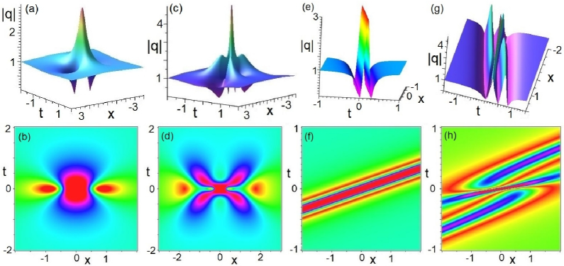
Figure 1: (a,b) 1-order rogue wave of NLS equation; (c, d) 2-order rogue wave of NLS equation;(e,f) 1-order rational soliton $q^{(1)}(x,t)$ of c-mKdV equation; (g, h) 2-order rational soliton $q^{(2)}(x,t)$ of c-mKdV equation.

Remark 1.1.

The W-shaped rational solitons of the c-mKdV equation differ from the rational rogue waves of the NLS equation even if they are both nonzero backgrounds. Moreover, these rational solitons also differ from the usual solitons with zero background.

Remark 1.2.

When the initial condition is taken as $q(x,0)=e^{i\sqrt{6}x}$, multi-rogue waves of the c-mKdV equation (1.3) can be found [95]

$$q_{cmkdv}(x,t)=\left[1-\frac{4(1-12\sqrt{6}it)}{4(x+12t)^{2}+432t^{2}+1}\right]e^{i\sqrt{6}x},$$ (1.5)

which differs from the W-shaped rational soliton $q_{cmkdv}^{[1]}(x,t)$ of the c-mKdV equation (1.3) gvien by Eq. (1.4).

Recently, Chen and Yan [22] found the $(2n-1,2n)$th-order RW solutions and rational solitons of both the Hirota equation and c-mKdV equation (1.3) with non-zero boundary conditions, respectively, via the robust IST and RHPs [11]. Weng et al [86] found multi-rational solitons of $n$-component c-mKdV equations. Recently, Wang et al [84] and Zhang et al[96] studied the long-time asymptotics of the c-mKdV equation (1.3) with step-like initial data and Schwartz decaying initial data, respectively.

Moreover, the Painlevé equation hierarchy is an important aspect of the study of integrable systems [2], and each Painlevé equation can be written as the following compatibility condition for the Lax pair [37, 75]:

$${}\phi_{x}(x,\lambda)=A(x,\lambda)\phi(x,\lambda),\quad\phi_{\lambda}(x,\lambda)=B(x,\lambda)\phi(x,\lambda),$$

where

$${}A(x,\lambda)=\sum\limits_{k=0}^{L+l}A_{k}\lambda^{L-k},\quad B(x,\lambda)=\sum\limits_{k=0}^{N+n}B_{k}\lambda^{N-k},$$

and $A_{k}$ and $B_{k}$ are matrices with terms that depend on the solution of the Painlevé equation.

In recent years, extreme rational soliton (e.g., rational rogue wave) phenomena with huge energies have been verified theoretically and/or experimentally in many fields [51], such as ocean [35], nonlinear optics [77], Bose-Einstein condensation [16], finance [87], capillary waves [76], superfluid [41], cold atom [79] and plasma physics [68]. In particular, rational solitons including rational rogue waves have been verified to appear in some nonlinear integrable systems [33, 34, 2, 45], and nearly-integrable nonlinear wave equations [85, 78].

In this paper, we will focus on the large-order asymptotics of multi-rational solitons for the Cauchy problem of the focusing c-mKdV equation (1.3) with finite density initial conditions

$$q(x,0)=q_{0}(x),\quad\lim_{x\to\pm\infty}q_{0}(x)=q_{\pm},\quad\left|q_{\pm}\right|=q_{0}\neq 0$$ (1.6)

by analyzing the corresponding Riemann-Hilbert problems.

The c-mKdV equation has the plane wave solution

$$q_{cw}(x,t)=\alpha e^{i[kx-(k^{3}-6\alpha^{2}k)t+\vartheta]},\quad\alpha,\,k,\,\vartheta\in\mathbb{R}$$ (1.7)

As $k=0$, the plane wave is simplified as a nonzero constant, $q_{cw}(x,t)=\alpha e^{i\vartheta}$ with $\alpha\not=0$. Without loss of generality, we here take $q_{\pm}=q_{0}=1$ in Eq. (1.6). Moreover, we know that Eq. (1.3) has the solitary wave solution

$$q_{cmkdv}(x,t)=\alpha\,{\rm sech}[\alpha x-(\alpha^{3}-3k^{2}\alpha)t+c]e^{i[kx+(k^{3}-3\alpha^{2}k)t+\vartheta]},\quad\alpha,\,c,\,k,\,\vartheta\in\mathbb{R}$$ (1.8)

which approaches to $0$ as $|x|,|t|\to\infty$. The phase and group velocities of the plane wave (1.7) are $v_{pv}=k^{2}-6\alpha^{2}$ and $v_{gv}=3k^{2}-6\alpha^{2}$, respectively. However, phase and group velocities of the solitary wave (1.8) are $v_{pv}=-k^{2}+3\alpha^{2}$ and $v_{gv}=-3k^{2}+3\alpha^{2}$, respectively.

Remark 1.3.

The c-mKdV equation (1.3) is invariant under the scaling transform

$$x\to\gamma^{-1}x^{\prime},\quad t\to\gamma^{-3}t^{\prime},\quad q(x,t)\to\gamma e^{i\vartheta}q(x^{\prime},t^{\prime}),$$ (1.9)

where $\gamma\not=0$ is arbitrary real constants, and $\vartheta\in[0,2\pi)$.

For convenience, we introduce the following notations:

$$\sigma_{1}=\!\left[\!\!\begin{array}[]{cc}0&1\vskip 3.61371pt\\ 1&0\end{array}\!\!\right],\quad\sigma_{2}=\!\left[\!\!\begin{array}[]{cc}0&-i\vskip 3.61371pt\\ i&0\end{array}\!\!\right],\quad\sigma_{3}=\!\left[\!\!\begin{array}[]{cc}1&0\vskip 3.61371pt\\ 0&-1\end{array}\!\!\right],\quad Q=\!\dfrac{\sqrt{2}}{2}\left[\!\!\begin{array}[]{cc}1&-1\vskip 3.61371pt\\ 1&1\end{array}\!\!\right].$$ (1.18)

Eq. (1.3) possesses the Lax pair:

$$\left\{\begin{aligned} \psi_{x}=&\,(-i\lambda\sigma_{3}+U)\psi=\left[\!\!\begin{array}[]{cc}-i\lambda&q\vskip 3.61371pt\\ -q^{*}&i\lambda\end{array}\!\!\right]\psi,\quad U=\!\left[\!\!\begin{array}[]{cc}0&q(x,t)\vskip 3.61371pt\\ -q^{*}(x,t)&0\end{array}\!\!\right],\vskip 7.22743pt\\ \psi_{t}=&\,(-4i\lambda^{3}\sigma_{3}+W)\psi=\left[\!\!\begin{array}[]{cc}-4i\lambda^{3}+2i\lambda|q|^{2}+q_{x}^{*}q-q_{x}q^{*}&4\lambda^{2}q+2i\lambda q_{x}-q_{xx}-2|q|^{2}q\vskip 3.61371pt\\ -4\lambda^{2}q^{*}+2i\lambda q_{x}^{*}+q_{xx}^{*}+2|q|^{2}q^{*}&4i\lambda^{3}-2i\lambda|q|^{2}-q_{x}^{*}q+q_{x}q^{*}\end{array}\!\!\right]\psi,\vskip 7.22743pt\\ &W=4\lambda^{2}U-2i\lambda(U_{x}+U^{2})\sigma_{3}+[U_{x},U]+2U^{3}-U_{xx},\end{aligned}\right.$$ (1.19)

where $\psi=\psi(x,t;\lambda)$ is an unknown $2\times 2$ matrix-valued eigenfunction, $\lambda\in\mathbb{C}$ is a spectral parameter, that is, Eq. (1.3) is viewed as the compatibility condition of the Lax pair.

We here review some basic properties about the robust IST of the c-mKdV equation (1.3) [3, 22]. According to the boundary conditions $\lim\limits_{x\rightarrow\pm\infty}q(x,t)=1$, the Lax pair (1.19) becomes

$$\left\{\begin{aligned} \psi_{x}^{bg}=&\,(-i\lambda\sigma_{3}+U^{bg})\psi^{bg},\quad U^{bg}=\!\left[\!\!\begin{array}[]{cc}0&1\vskip 3.61371pt\\ -1&0\end{array}\!\!\right],\vskip 7.22743pt\\ \psi_{t}^{bg}=&\,\left(-4i\lambda^{3}\sigma_{3}+4\lambda^{2}U^{bg}-2i\lambda(U^{bg})^{2}\sigma_{3}+2(U^{bg})^{3}\right)\psi^{bg},\end{aligned}\right.$$ (1.20)

which has the following fundamental solution matrix:

$$\psi^{bg}(\lambda;x,t)=E(\lambda)e^{-i\rho(\lambda)\big{(}x+(4\lambda^{2}-2)t\big{)}\sigma_{3}},$$ (1.21)

where

$$E(\lambda)=\!w(\lambda)\left[\!\!\begin{array}[]{cc}1&i(\lambda-\rho(\lambda))\vskip 3.61371pt\\ i(\lambda-\rho(\lambda))&1\end{array}\!\!\right],\quad\rho^{2}(\lambda)=\lambda^{2}+1,\quad w^{2}(\lambda)=\frac{\lambda+\rho(\lambda)}{2\rho(\lambda)},$$ (1.24)

which is a two-sheeted Riemann surface for $\lambda$, and $\rho(\lambda)=\lambda+\mathcal{O}(\lambda^{-1}),\quad\lambda\rightarrow\infty$ such that $\lim_{\lambda\to\infty}w(\lambda)=1$. Then, we have ${\rm det}(E(\lambda))={\rm det}(Q)=1.$

It can be easy to find the unique Jost solutions $\psi_{\pm}(\lambda;x,t)$ of Lax pair (1.19):

$$\psi_{\pm}(\lambda;x,t)=\mu_{\pm}(\lambda;x,t)e^{-i\rho(\lambda)(x+(4\lambda^{2}-2)t)\sigma_{3}},$$ (1.25)

with

$$\psi_{\pm}(\lambda;x,t)e^{i\rho(\lambda)(x+(4\lambda^{2}-2)t)\sigma_{3}}=E(\lambda)+o(1),\qquad x\to\pm\infty,$$ (1.26)

where

$$\mu_{\pm}(\lambda;x,t)=E(\lambda)+\int_{\pm\infty}^{x}E(\lambda)e^{-i\rho(\lambda)(x-y)\widehat{\sigma}_{3}}(E(\lambda)^{-1}\Delta q(y,t)\mu_{\pm}(\lambda;{\color[rgb]{1,0,0}y},t))dy$$ (1.27)

with $\Delta q(x,t)=\left[\!\!\begin{array}[]{cc}0&q(x,t)-1\vskip 3.61371pt\\ 1-q^{*}(x,t)&0\end{array}\!\!\right]$ and $e^{\widehat{\sigma}_{3}}\bullet=e^{\sigma_{3}}\bullet e^{-\sigma_{3}}$.

Let $\mu_{\pm j}$ stand for their $j$th column. Then, according to Eq. (1.27), it can be shown that $\mu_{-1}(\lambda;x,t),\mu_{+2}(\lambda;x,t)$ are bounded and analytic in $\mathbb{C}^{+}\setminus\Sigma_{c}$ and continuous up to the boundary ($\mathbb{C}^{+}$ is the upper half-plane of the complex $\lambda$-plane and $\Sigma_{c}=[-i,i]$), and $\mu_{+1}(\lambda;x,t),\mu_{-2}(\lambda;x,t)$ are bounded and analytic in $\mathbb{C}^{-}\setminus\Sigma_{c}$ and continuous up to the boundary ($\mathbb{C}^{-}$ is the lower half-plane of the complex $\lambda$-plane).

When $\lambda\in\mathbb{R}\cup\Sigma_{c}$, the Jost solutions $\psi_{\pm}(\lambda;x,t)$ have a relationship by a scattering matrix:

$$\psi_{+}(\lambda;x,t)=\psi_{-}(\lambda;x,t)S(\lambda),\qquad S(\lambda)=\left[\!\!\begin{array}[]{cc}s_{11}^{*}(\lambda^{*})&s_{12}^{*}(\lambda^{*})\vskip 3.61371pt\\ -s_{12}(\lambda)&s_{11}(\lambda)\end{array}\!\!\right].$$ (1.30)

Lemma 1.1.

[22, 11] For the fixed $L\in\mathbb{R}$, suppose that $q(x,t)$ is a bounded classical solution of Eq. (1.3) defined for $(x,t)$ in a simply connected domain $\Omega\subseteq\mathbb{R}$ which contains the point $(L,0)$. Then for each $\lambda\in\mathbb{C}$ there exists a unique simultaneous fundamental solution matrix $\psi=\psi^{\mathrm{in}}(x,t;\lambda)$, which satisfies Lax pairs (1.19) and the initial condition $\psi^{\mathrm{in}}(L,0;\lambda)=\mathbb{I}$. For each $(x,t)\in\Omega$, $\psi=\psi^{\mathrm{in}}(x,t;\lambda)$ is an entire function of $\lambda$ and ${\rm det}(\psi^{\mathrm{in}}(x,t;\lambda))=1$.

Let $\Sigma_{0}$ represent a clockwise circular contour centered on the origin and having a radius $r_{0}$ greater than 1. And let

$$M(x,t;\lambda)=\psi(x,t;\lambda)e^{i\rho(\lambda)(x+(4\lambda^{2}-2)t)\sigma_{3}},\quad\lambda\in\mathbb{C}\setminus(\Sigma_{0}\cup\Sigma_{c}),\quad(x,t)\in\mathbb{R}\times\mathbb{R}^{+},$$ (1.31)

with

$${}\psi(x,t;\lambda)=\begin{cases}\begin{array}[]{ll}\left(\!\!\begin{array}[]{cc}\dfrac{\psi_{-1}(x,t,\lambda)}{s_{11}(\lambda)},&\psi_{+2}(x,t,\lambda)\end{array}\!\!\right),&\lambda\in D_{+},\vskip 3.61371pt\\ \left(\!\!\begin{array}[]{cc}\psi_{+1}(x,t,\lambda),&\dfrac{\psi_{-2}(x,t,\lambda)}{s_{11}^{*}(\lambda^{*})}\end{array}\!\!\right),&\lambda\in D_{-},\vskip 3.61371pt\\ \psi^{\mathrm{in}}(x,t;\lambda),&\lambda\in D_{0},\end{array}\end{cases}$$

where $\Sigma_{+}:=\Sigma_{0}\cap\mathbb{C}^{+}$, $\Sigma_{-}:=\Sigma_{0}\cap\mathbb{C}^{-}$, $\Sigma_{l}:=\{\lambda\in\mathbb{R}\,\,|\,\,\lambda\leq-r_{0}\}$,  $\Sigma_{r_{0}}:=\{\lambda\in\mathbb{R}\,\,|\,\,\lambda\geq r_{0}\}$, $D_{0}:=\{\lambda\in\mathbb{C}\,\,|\,\,|\lambda|<r_{0}\}$, $D_{+}:=\{\lambda\in\mathbb{C}\,\,|\,|\lambda|>r_{0}\}\cap\mathbb{C}^{+}$,  $D_{-}:=\{\lambda\in\mathbb{C}\,\,|\,\,|\lambda|>r_{0}\}\cap\mathbb{C}^{-}$.

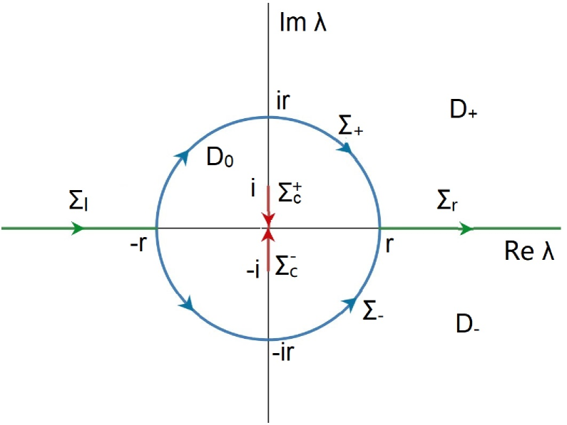
Figure 2: The jump contour $\Sigma_{l}\cup\Sigma_{r}\cup\Sigma_{+}\cup\Sigma_{-}\cup\Sigma_{c}$ for $M(x,t,\lambda)$ [22].

Lemma 1.2.

[22] The modified Riemann-Hilbert problem of the c-mKdV equation (1.3), that is,

• Analyticity: $M(x,t;\lambda)$ is a meromorphic function in $\lambda\in\mathbb{C}\setminus(\Sigma_{l}\cup\Sigma_{r}\cup\Sigma_{0}\cup\Sigma_{c})$;

• Jump conditions: The boundary values on the jump contour $\Sigma_{l}\cup\Sigma_{r}\cup\Sigma_{0}\cup\Sigma_{c}$ are related as:

  $${}M_{+}(x,t;\lambda)=M_{-}(x,t;\lambda)V(x,t;\lambda).$$

• Normalization: $M(x,t;\lambda)={\color[rgb]{1,0,0}\mathbb{I}}+\mathcal{O}(\lambda^{-1})$ as $\lambda\rightarrow\infty$.

where the jump contour is given in Fig. 2, and the jump matrix $V(x,t;\lambda)$ is defined by

$${}V(x,t;\lambda)=\begin{cases}e^{-i\rho(\lambda)(x+(4\lambda^{2}-2)t)\widehat{\sigma}_{3}}V_{1}(\lambda),\quad\lambda\in\Sigma_{0},\vskip 3.61371pt\\ e^{2i\rho_{+}(\lambda)(x+(4\lambda^{2}-2)t)\sigma_{3}},\quad\lambda\in\Sigma_{c},\end{cases}$$

with

$${}V_{1}(\lambda)=\begin{cases}\left(\!\!\begin{array}[]{cc}\dfrac{\psi_{-1}(L,0;\lambda)}{s_{11}(\lambda)},&\psi_{+2}(L,0;\lambda)\end{array}\!\!\right),\quad\lambda\in D_{+},\vskip 7.22743pt\\ \left(\!\!\begin{array}[]{cc}\psi_{+1}(L,0;\lambda),&\dfrac{\psi_{-2}(L,0;\lambda)}{s_{11}^{*}(\lambda^{*})}\end{array}\!\!\right)^{-1},\quad\lambda\in D_{-},\vskip 7.22743pt\\ \left[\!\!\begin{array}[]{cc}1+|\hat{r}(\lambda)|^{2}&\hat{r}^{*}(\lambda)\vskip 3.61371pt\\ \hat{r}(\lambda)&1\end{array}\!\!\right],\qquad\lambda\in\Sigma_{l}\cup\Sigma_{r},\quad\hat{r}(\lambda)=\dfrac{s_{12}(\lambda)}{s_{11}(\lambda)},\end{cases}$$

has a unique solution $M(x,t;\lambda)$ for $(x,t)\in\mathbb{R}\times\mathbb{R}^{+}$.

Then, the solution of c-mKdV equation (1.3) can be given by the solution $M(x,t;\lambda)$:

$${}q(x,t)=2i\lim_{\lambda\rightarrow\infty}\lambda M_{12}(x,t;\lambda).$$

We consider the following gauge transformation:

$${}\widehat{\psi}(x,t;\lambda)=\begin{cases}G(x,t;\lambda)\psi(x,t;\lambda),\quad\lambda\in D_{+}\cup D_{-},\vskip 3.61371pt\\ G(x,t;\lambda)\psi(x,t;\lambda)G(L,0;\lambda)^{-1},\quad\lambda\in D_{0}.\end{cases}$$

By adjusting the parameters in function $G(x,t;\lambda)$ and performing multiple gauge transformations, higher-order rational soliton solutions of c-mKdV equation (1.3) can be obtained. Thus one can find the $(2n-1,\,2n)$th-order rational soliton solution of Eq. (1.3) in the form [22]

$$\begin{array}[]{l}\tilde{q}_{0/e}(x,t)=1+2i\dfrac{\rm{det}({\mathcal{P}}_{o/e,4n}(x,t))+\rm{det}({\mathcal{P}}_{o/e,4n-1}(x,t))}{\rm{det}({\mathcal{P}}_{o/e}(x,t))},\end{array}$$ (1.33)

where $\mathcal{P}_{o/e}(x,t)=\mathcal{P}_{(2n-1)/(2n)}(x,t)$ is a coefficient matrix that consists of $2n\times 2n$ blocks:

$$\mathcal{P}_{o/e}(x,t)=$$

$$\left(\!\!\!\begin{array}[]{cccccccc}A^{[1]}_{0}&A^{[2]}_{0}&0&0&\cdots&\cdots&\cdots&0\vskip 7.22743pt\\ A^{[1]}_{1}&A^{[2]}_{1}&A^{[1]}_{0}&A^{[2]}_{0}&0&\cdots&\cdots&0\vskip 7.22743pt\\ \vdots&\vdots&\vdots&\vdots&\vdots&\vdots&\vdots&\vdots\vskip 7.22743pt\\ A^{[1]}_{n-1}&A^{[2]}_{n-1}&A^{[1]}_{n-2}&A^{[2]}_{n-2}&\cdots&\cdots&A^{[1]}_{0}&A^{[2]}_{0}\vskip 7.22743pt\\ A^{[1]}_{n}+B^{[1]}_{0,n}&A^{[2]}_{n}+B^{[2]}_{0,n}&A^{[1]}_{n-1}+B^{[1]}_{0,n-1}&A^{[2]}_{n-1}+B^{[2]}_{0,n-1}&\cdots&\cdots&A^{[1]}_{1}+B^{[1]}_{0,1}&A^{[2]}_{1}+B^{[2]}_{0,1}\vskip 7.22743pt\\ A^{[1]}_{n+1}+B^{[1]}_{1,n}&A^{[2]}_{n+1}+B^{[2]}_{1,n}&A^{[1]}_{n}+B^{[1]}_{1,n-1}&A^{[2]}_{n}+B^{[2]}_{1,n-1}&\cdots&\cdots&A^{[1]}_{2}+B^{[1]}_{1,1}&A^{[2]}_{2}+B^{[2]}_{1,1}\vskip 7.22743pt\\ A^{[1]}_{n+2}+B^{[1]}_{2,n}&A^{[2]}_{n+2}+B^{[2]}_{2,n}&A^{[1]}_{n+1}+B^{[1]}_{2,n-1}&A^{[2]}_{n+1}+B^{[2]}_{2,n-1}&\cdots&\cdots&A^{[1]}_{3}+B^{[1]}_{2,1}&A^{[2]}_{3}+B^{[2]}_{2,1}\vskip 7.22743pt\\ \vdots&\vdots&\vdots&\vdots&\vdots&\vdots&\vdots&\vdots\vskip 7.22743pt\\ A^{[1]}_{2n-1}\!+\!B^{[1]}_{n-1,n}&A^{[2]}_{2n-1}\!+\!B^{[2]}_{n-1,n}&A^{[1]}_{2n-2}\!+\!B^{[1]}_{n-1,n-1}&A^{[2]}_{2n-2}\!+\!B^{[2]}_{n-1,n-1}&\cdots&\cdots&A^{[1]}_{n}\!+\!B^{[1]}_{n-1,1}&A^{[2]}_{n}\!+\!B^{[2]}_{n-1,1}\end{array}\!\!\!\right)$$ (1.43)

with

$${}A_{k}^{[j]}=\left(\begin{array}[]{cc}(w^{+}_{o/e,k}(x,t))_{j}&0\\ 0&(w^{-}_{o/e,k}(x,t))_{j}\end{array}\right),\quad j=1,2,$$ (1.46)

$${}B_{m,k}^{[j]}=:\left(\begin{array}[]{cc}0&\sum_{l=0}^{m}\gamma_{(m-l)k}(w^{+}_{o/e,l}(x,t))_{j}\\ \sum_{l=0}^{m}(-1)^{k+m-l}\gamma_{(m-l)k}(w^{-}_{o/e,l}(x,t))_{j}&0\end{array}\right),\quad j=1,2,$$ (1.49)

$\gamma_{km}=\frac{(-1)^{k}}{(2i)^{m+k}}\left(\begin{array}[]{c}m+k-1\\ k\end{array}\right)$,  $(m=1,2,\ldots;\,k=0,1,\ldots),$ $w^{+}_{o/e,k}(x,t)=D_{k}^{+}(x,t){\bf c}_{\infty,o/e}$ and $w^{-}_{o/e,k}(x,t)=D_{k}^{-}(x,t)\sigma_{3}{\bf c}_{\infty,o/e},\,k=0,1,2,\ldots$ with $D_{k}^{+}(x,t)$, $D_{k}^{-}(x,t)$ being the Taylor coefficients of the analytic function $\psi_{bg}(\lambda;x,t)\psi_{bg}(\lambda;0,0)^{-1}$ in $\lambda=\pm i$, i.e., $\Psi^{in}_{bg}(\lambda;x,t)=\sum_{j=0}^{\infty}D_{j}^{\pm}(x,t)(\lambda\mp i)^{j},$ and $\mathcal{P}_{o/e,k}$ stands for the matrix $\mathcal{P}_{o/e}$ with its $k$th column replaced by the vector $(0,\cdots,0,-(w^{+}_{o/e,0}(x,t))_{1},-(w^{-}_{o/e,0}(x,t))_{1},-(w^{+}_{o/e,1}(x,t))_{1},-(w^{-}_{o/e,1}(x,t))_{1}$, $\cdots$, $-(w^{+}_{o/e,n-1}(x,t))_{1},-(w^{-}_{o/e,n-1}(x,t))_{1})^{T}$, the signs $(\cdot)_{o}$ and $(\cdot)_{e}$ correspond to the data ${\bf c}_{\infty}=(1,-1)^{T}$ and ${\bf c}_{\infty}=(1,1)^{T}$, respectively (see Ref.  [22] for specific parameters).

It should be worth noting that though the c-mKdV equation (1.3) and the NLS equation possesses the same ZS spectral problem, but the temporal parts of their Lax pairs are distinct such that the NLS equation admits the multi-rational RWs with finite numbers of extreme points, but the c-mKdV equation possesses the multi-rational solitons with infinitely many extreme points (see. Fig. 1). Compared with the NLS equation, the phase function of the c-mKdV equation is different and has a higher degree, resulting in more asymptotic regions. The properties of limiting functions require more techniques and models to be proposed. Some highlights for the higher-order rational solitons are found for the Cauchy problem of the c-mKdV equation:

• The form of the obtained multi-rational soliton of the c-mKdV equation given by Eq. (1.33) is very difficult to directly analyze the large $N$-order asymptotics. We here use the Riemann-Hilbert problems to reconstruct multi-rational soliton solutions of the c-mKdV equation through a series of deformations to analyze the relevant properties of solution (see Proposition  2.3 with RHP 2).

• Through the scale transform of spatio-tempotal variables and spectral parameter: $\{X:=nx,\,T:=n^{3}t,\,\Lambda:=\frac{\lambda}{n}\}$, we construct the Riemann-Hilbert problem corresponding to the limit functions of the multi-rational soliton solutions of the c-mKdV equation (1.3). In order to analyze the PDE satisfied by the limit functions, we need to overcome the difficulties caused by the time part of the Riemann-Hilbert problem corresponding to the limit functions. At this point, we need to use higher-order constraints on the spatial part and take many computational techniques. As a result, Eq. (2.100) show that the limit functions satisfy the new complex mKdV equation (1.52) in the $(X,T)$-space.

• The Riemann-Hilbert problem corresponding to the limit functions of the c-mKdV equation is of odd power with respect to time variable, which affects the properties of the limit functions. In order to analyze the symmetries of the limit functions (see Propositions 3.4 and 3.5), we need to provide a new deformation for the Riemann-Hilbert problem. As a result, we find that the limit functions of the multi-rational soliton solution of c-mKdV equation are real (see Proposition 3.5), which can also be reflected in the asymptotic part of the solution.

• Due to the difficulty caused by the term $e^{-i(\Lambda X+4\Lambda^{3}T)\sigma_{3}}$ in the Riemann-Hilbert problem, it is no longer easy to derive the ODEs satisfied by the limit functions. By using a series of analysis, we not only provide the ODEs (3.160) with respect to space $X$ for fixed variable $T$ satisfied by the limit functions, but also provide the ODEs (3.171) with respect to times $T$ for fixed variable $X$ satisfied by the limit functions. The ODEs with respect to space variable $X$ are identified with certain members of the Painlevé-III hierarchy (see Theorem 1.3).

• Because the phase function contains the high-power parameter $z$ related to the spectral parameter, the c-mKdV equation has five asymptotic regions. And due to the limit function has special symmetry (3.123) (the limit function is real), we need to use the Painlevé-II differential equation (4.333) to solve the leading term and error estimation of the limit function.

Main results

Our main conclusions of this paper are summarized as follows:

Theorem 1.1.

The Riemann-Hilbert Problem $3$ given by Proposition 2.4 has a unique solution $N^{\pm}(\Lambda;X,T)$ with ${\rm det}(N^{\pm}(\Lambda;X,T))=1$. For each compact subset $K\subset\mathbb{R}^{2}$,

$$\sup\limits_{|\Lambda|\neq 1,(X,T)\in K}||N^{{}^{\pm}}(\Lambda;x,t)||=C(K)<\infty.$$ (1.50)

The function

$$\widehat{q}^{\pm}(X,T)=2i\lim_{\Lambda\rightarrow\infty}\Lambda N^{\pm}_{12}(\Lambda;X,T)$$ (1.51)

is a global solution of the complex modified Korteweg-de Vries (c-mKdV) equation:

$$\frac{\partial\widehat{q}}{\partial T}+\frac{\partial^{3}\widehat{q}}{\partial X^{3}}+6|\widehat{q}|^{2}\frac{\partial\widehat{q}}{\partial X}=0,\quad\widehat{q}=\widehat{q}(X,T).$$ (1.52)

Theorem 1.2.

Let $q_{k}(x,t)$ be the $k$th-order rational soliton of the c-mKdV equation (1.3) given by the formula (1.33). Then, if $k=2n,n\in\mathbb{N}$, one has

$$\frac{1}{n}q_{2n}\left(x,\,t\right)=\frac{1}{n}q_{2n}\left(\frac{X}{n},\,\frac{T}{n^{3}}\right)=\widehat{q}^{+}(X,T)+\mathcal{O}\left(\frac{1}{n}\right),\quad n\rightarrow\infty,$$ (1.53)

if $k=2n-1,n\in\mathbb{N}_{+}$, one has

$$\frac{1}{n}q_{2n-1}\left(x,\,t\right)=\frac{1}{n}q_{2n-1}\left(\frac{X}{n},\,\frac{T}{n^{3}}\right)=\widehat{q}^{-}(X,T)+\mathcal{O}\left(\frac{1}{n}\right),\quad n\rightarrow\infty,$$ (1.54)

uniformly for $(X,T)$ in compact subsets of $\mathbb{R}^{2}$, where $\widehat{q}^{\pm}(X,T)$ satisfies the c-mKdV Eq. (1.52).

Theorem 1.3.

The limit function $\widehat{q}^{\pm}(X,T)$ as a function of $X$ satisfies the following ordinary differential equations for fixed variable $T$:

$$\begin{aligned} &3\widehat{q}\widehat{q}_{XX}-2\widehat{q}_{X}^{2}+4\widehat{q}^{4}+X(\widehat{q}\widehat{q}_{XXX}-\widehat{q}_{X}\widehat{q}_{XX}+4\widehat{q}^{3}\widehat{q}_{X})\vskip 3.61371pt\\ &+3T\bigg{(}\widehat{q}_{X}\widehat{q}_{XXXX}-\widehat{q}\widehat{q}_{XXXXX}-6\widehat{q}^{2}(\widehat{q}\widehat{q}_{XX})_{x}-24\widehat{q}^{2}\widehat{q}_{X}\widehat{q}_{XX}-4\widehat{q}^{3}\widehat{q}_{XXX}-24\widehat{q}^{5}\widehat{q}_{X}\bigg{)}=0,\vskip 3.61371pt\\ &\bigg{(}\left(\widehat{q}+X\widehat{q}_{X}-3T\widehat{q}_{XXX}-18T\widehat{q}^{2}\widehat{q}_{X}\right)_{X}\bigg{)}^{2}+4\widehat{q}^{2}\left(\widehat{q}+X\widehat{q}_{X}-3T\widehat{q}_{XXX}-18T\widehat{q}^{2}\widehat{q}_{X}\right)^{2}-64\widehat{q}^{2}=0.\end{aligned}$$ (1.55)

When $T=0$, Eq. (3.149) becomes

$$\begin{aligned} &H_{X}(\Lambda;X,0)=\left[\!\!\begin{array}[]{cc}-i\Lambda&\widehat{q}(X,0)\vskip 3.61371pt\\ -\widehat{q}(X,0)&i\Lambda\end{array}\!\!\right]H(\Lambda;X,0),\vskip 3.61371pt\\ &H_{\Lambda}(\Lambda;X,0)=\left[\!\!\begin{array}[]{cc}-iX-\dfrac{i(2\widehat{q}_{X}+X\widehat{q}_{XX})}{4\widehat{q}}\Lambda^{-2}&X\widehat{q}\Lambda^{-1}+\dfrac{i}{2}(\widehat{q}+X\widehat{q}_{X})\Lambda^{-2}\vskip 3.61371pt\\ -X\widehat{q}\Lambda^{-1}+\dfrac{i}{2}(\widehat{q}+X\widehat{q}_{X})\Lambda^{-2}&iX+\dfrac{i(2\widehat{q}_{X}+X\widehat{q}_{XX})}{4\widehat{q}}\Lambda^{-2}\end{array}\!\!\right]H(\Lambda;X,0),\end{aligned}$$ (1.56)

which is the Lax pair of first member of the Painlevé-III equation hierarchy.

And when $T=0$ and $f:=\partial_{X}\ln\widehat{q}(X,0)$, Eq. (3.160) can be written as

$$X^{2}(ff_{XX}-f_{X}^{2}-f^{4})+X(f_{XX}+ff_{X}-3f^{3})+3f_{X}-3f^{2}+64=0{\color[rgb]{1,0,0}.}$$ (1.57)

Theorem 1.4.

The limit function $\widehat{q}^{\pm}(X,T)$ as a function of $T$ satisfies the following ordinary differential equations for fixed variable $X$:

$$\begin{aligned} &\widehat{q}+X\widehat{q}_{X}+3T\widehat{q}_{T}-2\beta=0,\vskip 3.61371pt\\ &4\alpha\widehat{q}+2\beta_{X}=0,\vskip 3.61371pt\\ &X\widehat{q}_{T}-3(\widehat{q}_{XX}+2\widehat{q}^{3})-3T(\widehat{q}_{XXT}+6\widehat{q}_{T}\widehat{q}^{2})+4\beta\widehat{q}^{2}-4\alpha\widehat{q}_{X}=0,\vskip 3.61371pt\\ &\alpha_{T}+2\beta(\widehat{q}_{XX}+2\widehat{q}^{3})=0,\vskip 3.61371pt\\ &\beta_{T}-2\alpha(\widehat{q}_{XX}+2\widehat{q}^{3})=0,\vskip 3.61371pt\\ &\alpha(X,T)^{2}+\beta(X,T)^{2}=4.\end{aligned}$$ (1.58)

Theorem 1.5.

Let $-1/96<a\leq 0$ and $\Theta(z;a):=z+4az^{3}+2z^{-1}$. Then we know that the solution of Eq. (1.52) has the large $X$ asymptotics ($\widehat{q}^{+}(X,T)=-\widehat{q}^{-}(X,T)$)

$$\widehat{q}^{+}(X,aX^{2})=\frac{\sqrt{2p}\cos(\phi(X,a))}{X^{\frac{3}{4}}\sqrt{6ab+b^{-3}}}+\mathcal{O}(X^{-1}),\quad X\rightarrow+\infty,$$ (1.59)

where

$${}\phi(X,a)=2X^{\frac{1}{2}}\Theta(b;a)-p\ln(24ab+4b^{-3})-\frac{p\ln(X)}{2}-2p\ln(2b)+\mathrm{arg}(\Gamma(ip))-2\pi p^{2}-\frac{\pi}{4}.$$

Theorem 1.6.

Let $a\rightarrow-1/96=:a_{c}$ and $\Theta(z;a):=4az^{3}+z+2z^{-1}$. If we assume that $a-a_{c}=\mathcal{O}(X^{-\frac{1}{3}})$, then we have the solution of Eq. (1.52) has the large $X$ asymptotics

$$\widehat{q}^{+}(X,aX^{2})=-\frac{4\cdot 3^{\frac{1}{3}}|\mathcal{V}_{1}(-96\cdot 3^{\frac{1}{3}}(a+\frac{1}{96})X^{\frac{1}{3}})|}{X^{\frac{2}{3}}}\sin(\phi(X,a))+\mathcal{O}(X^{-\frac{5}{6}}),\quad X\rightarrow+\infty,$$ (1.60)

where

$${}\phi(X,a)=-\frac{\ln(2)}{6\pi}\ln(X)+\frac{16}{3}X^{\frac{1}{2}}+64(a+\frac{1}{96})X^{\frac{1}{2}}+\mathrm{arg}(\mathcal{V}_{1}(-96\cdot 3^{\frac{1}{3}}(a+\frac{1}{96})X^{\frac{1}{3}}))-\frac{\ln(2)}{\pi}\ln(4\cdot 3^{-\frac{1}{3}}).$$

The rest of this paper is arranged as follows. In Sec. 2, we perform a series of deformations on the Riemann-Hilbert problem corresponding to infinite-order rational solitons of the c-mKdV equation (1.3), and we construct a Riemann-Hilbert problem corresponding to the limit function which is a new solution of the c-mKdV equation (1.3) in the rescaled variables, $X$ and $T$, and prove the existence and uniqueness of the Riemann-Hilbert problem’s solution. In Sec. 3, we analyze the properties of the limit functions $\widehat{q}^{\pm}(X,T)$, including the symmetry and ordinary differential equation it satisfies. In Sec. 4, we study the large $X$ and transitional asymptotic behaviors of $\widehat{q}^{\pm}(X,T)$. And we provide some results under the condition of large $T$. Finally, we give some conclusions in Sec. 5.

2 Large-order asymptotics of multi-rational solitons under NZB

Before we study the near-field asymptotics of multi-rational solitons of the c-mKdV equation with nonzero background (1.3), we firstly present some two Riemann-Hilbert problems (RHPs), and the multi-rational solutions of the c-mKdV equation (1.3) expressed by using the RHP 2.

Proposition 2.1.

Riemann-Hilbert Problem 1.
Let $(x,t)\in\mathbb{R}^{2}$ and $k\in\mathbb{N}$. Find a $2\times 2$ matrix $M^{(k)}(\lambda;x,t)$ that satisfies the following properties:

• Analyticity: $M^{(k)}(\lambda;x,t)$ is analytic in $\{\lambda|\lambda\in\mathbb{C}\setminus(\Sigma_{c}\cup\Sigma_{0})\}$ and takes continuous boundary values on $\Sigma_{c}\cup\Sigma_{0}$.

• Jump condition: The boundary values on the jump contour $\Sigma_{c}\cup\Sigma_{0}$ are defined as

  $$M^{(k)}_{+}(\lambda;x,t)=M^{(k)}_{-}(\lambda;x,t)V^{(k)}(\lambda;x,t),\quad\lambda\in\Sigma_{c}\cup\Sigma_{0},$$ (2.61)

  where the jump matrix is defined as

  $${}V^{(k)}=\left\{\begin{array}[]{ll}\!\!\!e^{2i\rho_{+}(\lambda)(x+(4\lambda^{2}-2)t)\sigma_{3}},&\lambda\in\Sigma_{c},\vskip 7.22743pt\\ \!\!\!e^{-i\rho(\lambda)(x+(4\lambda^{2}-2)t)\sigma_{3}}Q\left(\dfrac{\lambda-i}{\lambda+i}\right)^{n\sigma_{3}}Q^{-1}E(\lambda)e^{i\rho(\lambda)(x+(4\lambda^{2}-2)t)\sigma_{3}},&\lambda\in\Sigma_{0},\,\,k=2n,\,n\in\mathbb{N},\vskip 7.22743pt\\ \!\!\!e^{-i\rho(\lambda)(x+(4\lambda^{2}-2)t)\sigma_{3}}Q\left(\dfrac{\lambda+i}{\lambda-i}\right)^{n\sigma_{3}}Q^{-1}E(\lambda)e^{i\rho(\lambda)(x+(4\lambda^{2}-2)t)\sigma_{3}},&\lambda\in\Sigma_{0},\,\,k=2n-1,\,n\in\mathbb{N}_{+}.\end{array}\right.$$ (2.65)

• Normalization: $M^{(k)}(\lambda;x,t)$ tends to the identity matrix as $\lambda\rightarrow\infty$.

Then, the $k$th-order rational soliton solution of the c-mKdV equation (1.3) with with finite density initial conditions (1.6) can be given by the formula:

$$q(x,t)=q_{k}(x,t)=2i\lim_{\lambda\rightarrow\infty}\lambda M_{12}^{(k)}(\lambda;x,t),\quad k\in\mathbb{N}.$$ (2.66)

In particular, if $k=0$, then the solution of Riemann-Hilbert Problem 1 is

$$\begin{aligned} M^{(0)}(\lambda;x,t)=\begin{cases}E(\lambda),\quad\mathrm{if}~\lambda~\mathrm{exterior}~\mathrm{to}~\Sigma_{0},\vskip 3.61371pt\\ E(\lambda)e^{-i\rho(\lambda)(x+(4\lambda^{2}-2)t)\widehat{\sigma}_{3}}E(\lambda)^{-1},\quad\mathrm{if}~\lambda~\mathrm{in}~\mathrm{the}~\mathrm{interior}~\mathrm{of}~\Sigma_{0}.\end{cases}\end{aligned}$$ (2.67)

Let

$$\begin{aligned} \widehat{E}(\lambda;x,t)&:=E(\lambda)e^{-i\rho(\lambda)(x+(4\lambda^{2}-2)t)\sigma_{3}}E(\lambda)^{-1}\vskip 3.61371pt\\ &=\frac{(x+(4\lambda^{2}-2)t)\sin(\theta)}{\theta}\left[\!\!\begin{array}[]{cc}-i\lambda&1\vskip 3.61371pt\\ -1&i\lambda\end{array}\!\!\right]+\cos(\theta)\mathbb{I},\end{aligned}$$ (2.68)

with $\theta=\rho(\lambda)(x+(4\lambda^{2}-2)t)$. Then according to the formula (2.66), we have

$${}q_{0}(x,t)=2i\lim_{\lambda\rightarrow\infty}\lambda M_{12}^{(0)}(\lambda;x,t)=2i\lim_{\lambda\rightarrow\infty}\lambda E_{12}(\lambda)=1.$$

The Riemann-Hilbert Problem 1 without jump across $\Sigma_{c}$ is easily formulated. To this end, we will make the following transformation:

$$\widehat{M}^{(k)}(\lambda;x,t):=M^{(k)}(\lambda;x,t)M^{(0)}(\lambda;x,t)^{-1}.$$ (2.69)

Proposition 2.2.

Riemann-Hilbert Problem 2.
Let $(x,t)\in\mathbb{R}$ and $k\in\mathbb{N}$. Find a $2\times 2$ matrix $\widehat{M}^{(k)}(\lambda;x,t)$ defined by Eq. (2.69) that satisfies the following properties:

• Analyticity: $\widehat{M}^{(k)}(\lambda;x,t)$ is analytic in $\{\lambda|\lambda\in\mathbb{C}\setminus\Sigma_{0}\}$ and takes continuous boundary values on $\Sigma_{0}$ from both the exterior and interior.

• Jump conditions: The boundary values on the jump contour $\Sigma_{0}$ are defined as:
  if $k=2n,\,n\in\mathbb{N}$, then

  $$\begin{aligned} \widehat{M}^{(k)}_{+}(\lambda;x,t)=&\widehat{M}^{(k)}_{-}(\lambda;x,t)\widehat{E}(\lambda;x,t)Q\left(\frac{\lambda-i}{\lambda+i}\right)^{n\sigma_{3}}Q^{-1}\widehat{E}(\lambda;x,t)^{-1},\quad\lambda\in\Sigma_{0},\end{aligned}$$ (2.70)

  and if $k=2n-1,\,n\in\mathbb{N}_{+}$, then

  $$\begin{aligned} \widehat{M}^{(k)}_{+}(\lambda;x,t)=&\widehat{M}^{(k)}_{-}(\lambda;x,t)\widehat{E}(\lambda;x,t)Q\left(\frac{\lambda+i}{\lambda-i}\right)^{n\sigma_{3}}Q^{-1}\widehat{E}(\lambda;x,t)^{-1},\quad\lambda\in\Sigma_{0},\end{aligned}$$ (2.71)

  where the matrix $\widehat{E}(\lambda;x,t)$ is given by Eq. (2.68).

• Normalization: $\widehat{M}^{(k)}(\lambda;x,t)$ tends to the identity matrix $\mathbb{I}$ as $\lambda\rightarrow\infty$.

Proof.

If $\lambda\in\Sigma_{c}$, it follows from Eq. (2.69) that we have

$$\begin{aligned} \widehat{M}^{(k)}_{+}(\lambda;x,t)&=M^{(k)}_{+}(\lambda;,x,t)M^{(0)}_{+}(\lambda;,x,t)^{-1}\vskip 3.61371pt\\ &=M^{(k)}_{-}(\lambda;x,t)e^{2i\rho_{+}(\lambda)(x+(4\lambda^{2}-2)t)\sigma_{3}}\left(M^{(0)}_{-}(\lambda;x,t)e^{2i\rho_{+}(\lambda)(x+(4\lambda^{2}-2)t)\sigma_{3}}\right)^{-1}\vskip 3.61371pt\\ &=M^{(k)}_{-}(\lambda;x,t)M^{(0)}_{-}(\lambda;x,t)^{-1}\vskip 3.61371pt\\ &=\widehat{M}^{(k)}_{-}(\lambda;x,t)\mathbb{I}.\end{aligned}$$ (2.72)

This indicates that $\widehat{M}^{(k)}(\lambda;x,t)$ has no jump across $\Sigma_{c}$. According to the Riemann-Hilbert Problem 1 and Eq. (2.69), we know that $\widehat{M}^{(k)}(\lambda;x,t)$ is analytic in $\{\lambda|\lambda\in\mathbb{C}\setminus\Sigma_{0}\}$ and takes continuous boundary values on $\Sigma_{0}$ from both the exterior and interior.

If $\lambda\in\Sigma_{0},k=2n,n\in\mathbb{N}$, we have

$$\begin{aligned} \widehat{M}^{(k)}_{+}(\lambda;x,t)=&M^{(k)}_{+}(\lambda;,x,t)M^{(0)}_{+}(\lambda;,x,t)^{-1}\vskip 3.61371pt\\ =&M^{(k)}_{-}(\lambda;x,t)M^{(0)}_{-}(\lambda;x,t)^{-1}M^{(0)}_{-}(\lambda;x,t)e^{-i\rho(\lambda)(x+(4\lambda^{2}-2)t)\sigma_{3}}\vskip 3.61371pt\\ &\times Q\left(\frac{\lambda-i}{\lambda+i}\right)^{n\sigma_{3}}Q^{-1}E(\lambda)e^{i\rho(\lambda)(x+(4\lambda^{2}-2)t)\sigma_{3}}\vskip 3.61371pt\\ &\times\bigg{(}M^{(0)}_{-}(\lambda;x,t)e^{-i\rho(\lambda)(x+(4\lambda^{2}-2)t)\sigma_{3}}E(\lambda)e^{i\rho(\lambda)(x+(4\lambda^{2}-2)t)\sigma_{3}}\bigg{)}^{-1}\vskip 3.61371pt\\ =&\widehat{M}^{(k)}_{-}(\lambda;x,t)\widehat{E}(\lambda;x,t)Q\left(\frac{\lambda-i}{\lambda+i}\right)^{n\sigma_{3}}Q^{-1}\widehat{E}(\lambda;x,t)^{-1}.\end{aligned}$$ (2.73)

If $\lambda\in\Sigma_{0},k=2n-1,n\in\mathbb{N}_{+}$, then we have

$$\begin{aligned} \widehat{M}^{(k)}_{+}(\lambda;x,t)=&M^{(k)}_{+}(\lambda;,x,t)M^{(0)}_{+}(\lambda;,x,t)^{-1}\vskip 3.61371pt\\ =&M^{(k)}_{-}(\lambda;x,t)M^{(0)}_{-}(\lambda;x,t)^{-1}M^{(0)}_{-}(\lambda;x,t)e^{-i\rho(\lambda)(x+(4\lambda^{2}-2)t)\sigma_{3}}\vskip 3.61371pt\\ &\times Q\left(\frac{\lambda+i}{\lambda-i}\right)^{n\sigma_{3}}Q^{-1}E(\lambda)e^{i\rho(\lambda)(x+(4\lambda^{2}-2)t)\sigma_{3}}\vskip 3.61371pt\\ &\times\bigg{(}M^{(0)}_{-}(\lambda;x,t)e^{-i\rho(\lambda)(x+(4\lambda^{2}-2)t)\sigma_{3}}E(\lambda)e^{i\rho(\lambda)(x+(4\lambda^{2}-2)t)\sigma_{3}}\bigg{)}^{-1}\vskip 3.61371pt\\ =&\widehat{M}^{(k)}_{-}(\lambda;x,t)\widehat{E}(\lambda;x,t)Q\left(\frac{\lambda+i}{\lambda-i}\right)^{n\sigma_{3}}Q^{-1}\widehat{E}(\lambda;x,t)^{-1}.\end{aligned}$$ (2.74)

Finally, according to Eq. (2.69), we know that $\widehat{M}^{(k)}(\lambda;x,t)\to\mathbb{I}$ as $\lambda\rightarrow\infty$. Thus the proof is completed. ∎

Proposition 2.3.

The solution of Eq. (1.3) with finite density initial conditions (1.6) can be expressed as:

$$q_{k}(x,t)=1+2i\lim_{\lambda\rightarrow\infty}\lambda\widehat{M}_{12}^{(k)}(\lambda;x,t),\quad k\in\mathbb{N},$$ (2.75)

where $\widehat{M}^{(k)}(\lambda;x,t)$ satisfies the Riemann-Hilbert Problem 2.

Proof.

According to Eq. (2.66), we obtain

$$\begin{aligned} q_{k}(x,t)&=2i\lim_{\lambda\rightarrow\infty}\lambda M_{12}^{(k)}(\lambda;x,t),\quad k\in\mathbb{N}\vskip 3.61371pt\\ &=2i\lim_{\lambda\rightarrow\infty}\lambda\left(\widehat{M}^{(k)}(\lambda;x,t)M^{(0)}(\lambda;,x,t)\right)_{12}\vskip 3.61371pt\\ &=2i\lim_{\lambda\rightarrow\infty}\lambda\left(\widehat{M}_{11}^{(k)}(\lambda;x,t)M^{(0)}_{12}(\lambda;,x,t)+\widehat{M}_{12}^{(k)}(\lambda;x,t)M^{(0)}_{22}(\lambda;,x,t)\right)\vskip 3.61371pt\\ &=1+2i\lim_{\lambda\rightarrow\infty}\lambda\widehat{M}_{12}^{(k)}(\lambda;x,t).\end{aligned}$$ (2.76)

Thus the proof is completed. ∎

Now we consider the near-field asymptotics of rational solitons of the c-mKdV equation (1.3) with finite density initial conditions (1.6). We will perform the following scale transforms for the Riemann-Hilbert Problem 2:

$$X:=nx,\qquad T:=n^{3}t,\qquad\Lambda:=\frac{\lambda}{n}.$$ (2.77)

We choose a radius of $n$ for the contour $\Sigma_{0}$, then the jump matrix possesses the following asymptotic behavior:

$$\begin{aligned} &\widehat{E}(\lambda;x,t)Q\left(\dfrac{\lambda-i}{\lambda+i}\right)^{\pm n\sigma_{3}}Q^{-1}\widehat{E}(\lambda;x,t)^{-1}\vskip 3.61371pt\\ =~&E(\lambda)e^{-i\rho(\lambda)(x+(4\lambda^{2}-2)t)\sigma_{3}}E(\lambda)^{-1}Q\left(\dfrac{\lambda-i}{\lambda+i}\right)^{\pm n\sigma_{3}}Q^{-1}E(\lambda)e^{i\rho(\lambda)(x+(4\lambda^{2}-2)t)\sigma_{3}}E(\lambda)^{-1}\vskip 3.61371pt\\ =~&\left(\mathbb{I}+\mathcal{O}\left(\frac{1}{n}\right)\right)e^{-i(\Lambda X+4\Lambda^{3}T)\sigma_{3}}Qe^{\mp 2i\Lambda^{-1}\sigma_{3}}Q^{-1}e^{i(\Lambda X+4\Lambda^{3}T)\sigma_{3}},\quad n\to\infty,\end{aligned}$$ (2.78)

which holds uniformly for $|\Lambda|=1$ and $(X,T)$ in compact subsets of $\mathbb{R}^{2}$.

Proposition 2.4.

Riemann-Hilbert Problem 3.
Let $(X,T)$ be in compact subsets of $\mathbb{R}^{2}$. Find a $2\times 2$ matrix $N^{\pm}(\Lambda;X,T)$ that satisfies the following properties:

• Analyticity: $N^{\pm}(\Lambda;X,T)$ is analytic in $\mathbb{C}\setminus\Sigma_{1}:=\{\Lambda|~|\Lambda|\neq 1,\Lambda\in\mathbb{C}\}$ and takes continuous boundary values on $\Sigma_{1}:=\{\Lambda|~|\Lambda|=1,\Lambda\in\mathbb{C}\}$.

• Jump condition: Assuming clockwise orientation of $\Sigma_{1}$, the boundary values on the jump contour $\Sigma_{1}$ are related as:

  $$\begin{aligned} N^{\pm}_{+}(\Lambda;X,T)=&N^{\pm}_{-}(\Lambda;X,T)e^{-i(\Lambda X+4\Lambda^{3}T)\sigma_{3}}Qe^{\mp 2i\Lambda^{-1}\sigma_{3}}Q^{-1}e^{i(\Lambda X+4\Lambda^{3}T)\sigma_{3}},\quad\Lambda\in\Sigma_{1},\end{aligned}$$ (2.79)

• Normalization: $N^{\pm}(\Lambda;X,T)$ tends to the identity matrix $\mathbb{I}$ as $\Lambda\rightarrow\infty$.

Then, we will solve the Riemann-Hilbert Problem 3 and provide the proof of Theorem 1.1.

Proof.

To show solvability and uniqueness, we will prove that the jump matrices and the jump conditions in Riemann-Hilbert problem 3 satisfy the hypotheses of Zhou’s vanishing lemma [97]. For this reason, we reorient the jump contour $\Sigma_{1}$ to the upper half-plane in a clockwise orientation and the lower half-plane in a counterclockwise orientation. Then, we define the following piecewise function:

$$\begin{aligned} &V^{\pm}(\Lambda;X,T)=\begin{cases}e^{-i(\Lambda X+4\Lambda^{3}T)\sigma_{3}}Qe^{\mp 2i\Lambda^{-1}\sigma_{3}}Q^{-1}e^{i(\Lambda X+4\Lambda^{3}T)\sigma_{3}},\quad|\Lambda|=1,\,\,\mathrm{Im}(\Lambda)>0,\vskip 3.61371pt\\ e^{-i(\Lambda X+4\Lambda^{3}T)\sigma_{3}}Qe^{\pm 2i\Lambda^{-1}\sigma_{3}}Q^{-1}e^{i(\Lambda X+4\Lambda^{3}T)\sigma_{3}},\quad|\Lambda|=1,\,\,\mathrm{Im}(\Lambda)<0.\end{cases}\end{aligned}$$ (2.80)

For $|\Lambda|=1,\mathrm{Im}(\Lambda)>0$, since $Q^{-1}=Q^{T}$, thus we have

$$\begin{aligned} V^{\pm}(\Lambda;X,T)&=e^{-i(\Lambda X+4\Lambda^{3}T)\sigma_{3}}Qe^{\mp 2i\Lambda^{-1}\sigma_{3}}Q^{-1}e^{i(\Lambda X+4\Lambda^{3}T)\sigma_{3}}\vskip 3.61371pt\\ &=\left(e^{i(\Lambda^{*}X+4\Lambda^{*3}T)\sigma_{3}}Qe^{\pm 2i\Lambda^{*-1}\sigma_{3}}Q^{-1}e^{-i(\Lambda^{*}X+4\Lambda^{*3}T)\sigma_{3}}\right)^{*}\vskip 3.61371pt\\ &=\left(e^{-i(\Lambda^{*}X+4\Lambda^{*3}T)\sigma_{3}}Qe^{\pm 2i\Lambda^{*-1}\sigma_{3}}Q^{-1}e^{i(\Lambda^{*}X+4\Lambda^{*3}T)\sigma_{3}}\right)^{{\dagger}}\vskip 3.61371pt\\ &=\left(V^{\pm}(\Lambda^{*};X,T)\right)^{{\dagger}},\end{aligned}$$ (2.81)

where the superscript ${\dagger}$ denotes the conjugate transpose of the matrix. Considering the normalization condition $N^{\pm}(\Lambda;X,T)\rightarrow\mathbb{I}$ as $\Lambda\rightarrow\infty$, we have satisfied all the hypotheses of the vanishing lemma. Consequently, the Riemann-Hilbert problem 3 is uniquely solvable. The matrix $N^{\pm}(\Lambda;X,T)$ has the following Laurent expansion.

$$N^{\pm}(\Lambda;X,T)=\mathbb{I}+\sum_{j=1}^{\infty}N^{\pm[j]}(X,T)\Lambda^{-j},\quad|\Lambda|>1,$$ (2.82)

and analytic Fredholm theory implies that each $N^{\pm[j]}(X,T)$ is real analytic on $\mathbb{R}^{2}$. We will show that $\widehat{q}^{\pm}(X,T)$ is a global solution of the complex modified Korteweg-de Vries equation. To this end, we define

$${}P^{\pm}(\Lambda;X,T):=N^{\pm}(\Lambda;X,T)e^{-i(\Lambda X+4\Lambda^{3}T)\sigma_{3}}.$$

Then, $P^{\pm}(\Lambda;X,T)$ satisfies the following Riemann-Hilbert problem:

• Analyticity: $P^{\pm}(\lambda;X,T)$ is analytic in $\mathbb{C}\setminus\Sigma_{1}$ and takes continuous boundary values on $\Sigma_{1}$.

• Jump conditions: Assuming clockwise orientation of $\Sigma_{1}$, the boundary values on the jump contour $\Sigma_{1}$ are related as:

  $$P^{\pm}_{+}(\Lambda;X,T)=P^{\pm}_{-}(\Lambda;X,T)Qe^{\mp 2i\Lambda^{-1}\sigma_{3}}Q^{-1},\quad\Lambda\in\Sigma_{1},$$ (2.83)

• Normalization: $P^{\pm}(\Lambda;X,T)$ tends to $e^{-i(\Lambda X+4\Lambda^{3}T)}$ as $\Lambda\rightarrow\infty$.

We define two matrices:

$$\left\{\begin{aligned} &A^{\pm}(\Lambda;X,T):=P^{\pm}_{X}(\Lambda;X,T)P^{\pm}(\Lambda;X,T)^{-1},\vskip 3.61371pt\\ &B^{\pm}(\Lambda;X,T):=P^{\pm}_{T}(\Lambda;X,T)P^{\pm}(\Lambda;X,T)^{-1}.\end{aligned}\right.$$ (2.84)

They can be defined by continuity for $\Sigma_{1}$ and they are entire functions of $\Lambda$. Firstly, we provide the expression for $N^{\pm}(\Lambda;X,T)^{-1}$.

$$\begin{aligned} N^{\pm}(\Lambda;X,T)^{-1}=\,&\mathbb{I}-N^{\pm[1]}(X,T)\Lambda^{-1}+(N^{\pm[1]}(X,T)^{2}-N^{\pm[2]}(X,T))\Lambda^{-2}\vskip 3.61371pt\\ &+(N^{\pm[1]}(X,T)N^{\pm[2]}(X,T)+N^{\pm[2]}(X,T)N^{\pm[1]}(X,T)\vskip 3.61371pt\\ &-N^{\pm[3]}(X,T)-N^{\pm[1]}(X,T)^{3})\Lambda^{-3}+\mathcal{O}(\Lambda^{-4}),\quad\Lambda\rightarrow\infty.\end{aligned}$$ (2.85)

According to Eqs. (2.82), (2.84) and (2.85), we have

$$A^{\pm}(\Lambda;X,T)=-i\Lambda\sigma_{3}+i[\sigma_{3},N^{\pm[1]}(X,T)]+\mathcal{O}(\Lambda^{-1}),\quad\Lambda\rightarrow\infty,$$ (2.86)

and

$$\begin{aligned} B^{\pm}(\Lambda;X,T)=&-4i\Lambda^{3}\sigma_{3}+4i\Lambda^{2}[\sigma_{3},N^{\pm[1]}(X,T)]+4i\Lambda\bigg{(}[\sigma_{3}.N^{\pm[2]}(X,T)]\vskip 3.61371pt\\ &+[N^{\pm[1]}(X,T),\sigma_{3}N^{\pm[1]}(X,T)])+4i\bigg{(}[\sigma_{3},N^{\pm[3]}(X,T)]+[N^{\pm[2]}(X,T),\sigma_{3}N^{\pm[1]}(X,T)]\vskip 3.61371pt\\ &+[\sigma_{3}N^{\pm[1]}(X,T)^{2},N^{\pm[1]}(X,T)]+[N^{\pm[1]}(X,T),\sigma_{3}N^{\pm[2]}(X,T)]\bigg{)}+\mathcal{O}(\Lambda^{-1}),\quad\Lambda\rightarrow\infty.\end{aligned}$$ (2.87)

Using Liouville’s theorem, we get

$$\begin{aligned} A^{\pm}(\Lambda;X,T)=&-i\Lambda\sigma_{3}+i[\sigma_{3},N^{\pm[1]}(X,T)],\vskip 3.61371pt\\ B^{\pm}(\Lambda;X,T)=&-4i\Lambda^{3}\sigma_{3}+4i\Lambda^{2}[\sigma_{3},N^{\pm[1]}(X,T)]+4i\Lambda\bigg{(}[\sigma_{3},N^{\pm[2]}(X,T)]\vskip 3.61371pt\\ &+[N^{\pm[1]}(X,T),\sigma_{3}N^{\pm[1]}(X,T)]\bigg{)}+4i\bigg{(}[\sigma_{3},N^{\pm[3]}(X,T)]+[N^{\pm[2]}(X,T),\sigma_{3}N^{\pm[1]}(X,T)]\vskip 3.61371pt\\ &+[\sigma_{3}N^{\pm[1]}(X,T)^{2},N^{\pm[1]}(X,T)]+[N^{\pm[1]}(X,T),\sigma_{3}N^{\pm[2]}(X,T)]\bigg{)}.\end{aligned}$$ (2.88)

To eliminate matrices $N^{\pm[3]}(X,T)])$, we provide the error terms for $\Lambda^{-1}$ and $\Lambda^{-2}$ in Eq. (2.86).

$$P_{\Lambda^{-1}}:\quad i[\sigma_{3},N^{\pm[2]}(X,T)]+i[N^{\pm[1]}(X,T),\sigma_{3}N^{\pm[1]}(X,T)]+N_{X}^{\pm[1]}(X,T),$$ (2.89)

and

$$\begin{aligned} P_{\Lambda^{-2}}:\quad&i[\sigma_{3},N^{\pm[3]}(X,T)]+i[N^{\pm[2]}(X,T),\sigma_{3}N^{\pm[1]}(X,T)]+i[\sigma_{3}N^{\pm[1]}(X,T)^{2},N^{\pm[1]}(X,T)]\vskip 3.61371pt\\ &+i[N^{\pm[1]}(X,T),\sigma_{3}N^{\pm[2]}(X,T)]+N_{X}^{\pm[2]}(X,T)-N_{X}^{\pm[1]}(X,T)N^{\pm[1]}(X,T).\end{aligned}$$ (2.90)

Because of the existence and uniqueness of the solution to the Riemann-Hilbert problem 3, we have the following symmetric relation:

$$N^{\pm}(\Lambda;X,T)=\sigma_{2}N^{\pm}(\Lambda^{*};X,T)^{*}\sigma_{2}.$$ (2.91)

Note that $\widehat{q}^{\pm}(X,T)=2iN^{\pm[1]}_{12}(X,T)$ and solving $\{P_{\Lambda^{-1},11}=0,\,P_{\Lambda^{-1},22}=0\}$, we obtain

$$\left\{\begin{aligned} &N^{\pm[1]}_{11,X}(X,T)=-\frac{i}{2}|\widehat{q}^{\pm}(X,T)|^{2},\vskip 3.61371pt\\ &N^{\pm[1]}_{22,X}(X,T)=\frac{i}{2}|\widehat{q}^{\pm}(X,T)|^{2}.\end{aligned}\right.$$ (2.92)

Using Eqs. (2.87),(2.89) and(2.92), we have

$$\begin{aligned} B^{\pm}(\Lambda;X,T)=&-4i\Lambda^{3}\sigma_{3}+4i\Lambda^{2}[\sigma_{3},N^{\pm[1]}(X,T)]-4\Lambda N^{\pm[1]}_{X}(X,T)\vskip 3.61371pt\\ &+4i\bigg{(}[\sigma_{3},N^{\pm[3]}(X,T)]+[N^{\pm[2]}(X,T),\sigma_{3}N^{\pm[1]}(X,T)]\vskip 3.61371pt\\ &+[\sigma_{3}N^{\pm[1]}(X,T)^{2},N^{\pm[1]}(X,T)]+[N^{\pm[1]}(X,T),\sigma_{3}N^{\pm[2]}(X,T)\bigg{)}.\end{aligned}$$ (2.93)

To solve $\{P_{\Lambda^{-1},12}=0,\,P_{\Lambda^{-1},21}=0\}$, we have

$$\begin{aligned} &N^{\pm[2]}_{12}(X,T)=N^{\pm[1]}_{12}(X,T)N^{\pm[1]}_{22}(X,T)+\frac{i}{2}N^{\pm[1]}_{12,X}(X,T),\vskip 3.61371pt\\ &N^{\pm[2]}_{21}(X,T)=N^{\pm[1]}_{21}(X,T)N^{\pm[1]}_{11}(X,T)-\frac{i}{2}N^{\pm[1]}_{21,X}(X,T).\end{aligned}$$ (2.94)

Let

$${}\begin{aligned} M^{0}:=&[\sigma_{3},N^{\pm[3]}(X,T)]+[N^{\pm[2]}(X,T),\sigma_{3}N^{\pm[1]}(X,T)]+[\sigma_{3}N^{\pm[1]}(X,T)^{2},N^{\pm[1]}(X,T)]\vskip 3.61371pt\\ &+[N^{\pm[1]}(X,T),\sigma_{3}N^{\pm[2]}(X,T)].\end{aligned}$$

Extracting the elements of matrix $M^{0}$ at the diagonal, we have

$$\begin{aligned} M^{0}_{11}=&2N^{\pm[1]}_{12}(X,T)(N^{\pm[1]}_{21}(X,T)N^{\pm[1]}_{11}(X,T)+N^{\pm[1]}_{22}(X,T)N^{\pm[1]}_{21}(X,T))\vskip 3.61371pt\\ &-N^{\pm[2]}_{12}(X,T)N^{\pm[1]}_{21}(X,T)-N^{\pm[1]}_{12}(X,T)N^{\pm[2]}_{21}(X,T)\vskip 3.61371pt\\ &-N^{\pm[1]}_{12}(X,T)N^{\pm[2]}_{21}(X,T)-N^{\pm[2]}_{12}(X,T)N^{\pm[1]}_{21}(X,T),\vskip 3.61371pt\\ M^{0}_{22}=&-2N^{\pm[1]}_{21}(X,T)(N^{\pm[1]}_{11}(X,T)N^{\pm[1]}_{12}(X,T)+N^{\pm[1]}_{12}(X,T)N^{\pm[1]}_{22}(X,T))\vskip 3.61371pt\\ &+N^{\pm[2]}_{21}(X,T)N^{\pm[1]}_{12}(X,T)+N^{\pm[1]}_{21}(X,T)N^{\pm[2]}_{12}(X,T)\vskip 3.61371pt\\ &+N^{\pm[1]}_{21}(X,T)N^{\pm[2]}_{12}(X,T)+N^{\pm[2]}_{21}(X,T)N^{\pm[1]}_{12}(X,T).\end{aligned}$$ (2.95)

Substituting Eqs. (2.92) and (2.94) into Eq. (2.95), we obtain

$$\begin{aligned} &M^{0}_{11}=-\frac{i}{4}\widehat{q}^{\pm*}_{X}\widehat{q}^{\pm}+\frac{i}{4}\widehat{q}^{\pm}_{X}\widehat{q}^{\pm*},\vskip 3.61371pt\\ &M^{0}_{22}=\frac{i}{4}\widehat{q}^{\pm*}_{X}\widehat{q}^{\pm}-\frac{i}{4}\widehat{q}^{\pm}_{X}\widehat{q}^{\pm*}.\end{aligned}$$ (2.96)

Solving $\{P_{\Lambda^{-2},12}=0,\,P_{\Lambda^{-2},21}=0\}$, we obtain

$$\begin{aligned} &M^{0}_{12}=-iN^{\pm[1]}_{11,X}(X,T)N^{\pm[1]}_{12}(X,T)-iN^{\pm[1]}_{12,X}(X,T)N^{\pm[1]}_{22}(X,T)+iN^{\pm[2]}_{12,X}(X,T),\vskip 3.61371pt\\ &M^{0}_{21}=-iN^{\pm[1]}_{21,X}(X,T)N^{\pm[1]}_{11}(X,T)-iN^{\pm[1]}_{22,X}(X,T)N^{\pm[1]}_{21}(X,T)+iN^{\pm[2]}_{21,X}(X,T).\end{aligned}$$ (2.97)

Substituting Eqs. (2.92) and (2.94) into Eq. (2.97), we obtain

$$\begin{aligned} &M^{0}_{12}=\frac{i}{4}\widehat{q}^{\pm}_{XX}+\frac{i}{2}|\widehat{q}^{\pm}|^{2}\widehat{q}^{\pm},\vskip 3.61371pt\\ &M^{0}_{21}=-\frac{i}{4}\widehat{q}^{\pm*}_{XX}-\frac{i}{2}|\widehat{q}^{\pm}|^{2}\widehat{q}^{\pm*}.\end{aligned}$$ (2.98)

Substituting Eqs. (2.92), (2.94), (2.96), and (2.98) into Eq. (2.88), we have

$$\begin{aligned} &A^{\pm}(\Lambda;X,T)=\left[\!\!\begin{array}[]{cc}-i\Lambda&\widehat{q}^{\pm}(X,T)\vskip 3.61371pt\\ -\widehat{q}^{\pm}(X,T)^{*}&i\Lambda\end{array}\!\!\right],\vskip 3.61371pt\\ &B^{\pm}(\Lambda;X,T)=\left[\!\!\begin{array}[]{cc}-4i\Lambda^{3}+2i\Lambda|\widehat{q}^{\pm}|^{2}+\widehat{q}_{X}^{\pm*}\widehat{q}^{\pm}-\widehat{q}^{\pm}_{X}\widehat{q}^{\pm*}&4\Lambda^{2}\widehat{q}^{\pm}+2i\Lambda\widehat{q}^{\pm}_{X}-\widehat{q}^{\pm}_{XX}-2|\widehat{q}^{\pm}|^{2}\widehat{q}^{\pm}\vskip 3.61371pt\\ -4\Lambda^{2}\widehat{q}^{\pm*}+2i\Lambda\widehat{q}_{X}^{\pm*}+\widehat{q}_{XX}^{\pm*}+2|\widehat{q}^{\pm}|^{2}\widehat{q}^{\pm*}&4i\Lambda^{3}-2i\Lambda|\widehat{q}^{\pm}|^{2}-\widehat{q}_{X}^{\pm*}\widehat{q}^{\pm}+\widehat{q}^{\pm}_{X}\widehat{q}^{\pm*}\end{array}\!\!\right].\end{aligned}$$ (2.99)

Using Eqs. (2.92) and (2.99), we get the system of equations about the matrix functions $P^{\pm}(\Lambda;X,T)$:

$$\begin{aligned} &P_{X}^{\pm}(\Lambda;X,T)=A^{\pm}(\Lambda;X,T)P^{\pm}(\Lambda;X,T),\vskip 3.61371pt\\ &P_{T}^{\pm}(\Lambda;X,T)=B^{\pm}(\Lambda;X,T)P^{\pm}(\Lambda;X,T),\end{aligned}$$ (2.100)

which constitute the Lax pair for the c-mKdV equation. According to compatibility condition $A_{T}^{\pm}(\Lambda;X,T)-B_{X}^{\pm}(\Lambda;X,T)+[A^{\pm}(\Lambda;X,T),B^{\pm}(\Lambda;X,T)]=0$, we show that the function $q^{\pm}(X,T)$ is a solution of Eq. (1.52). Thus the proof is completed.

∎

Below we present the large-order asymptotic behavior of rational soliton solution $q_{k}(x,t)$ of the c-mKdV equation (1.3) with finite density initial conditions (1.6) after making a transformation (2.77). Our main result is given by the following Theorem. Firstly, we present a small-norm Riemann-Hilbert Problem.

Let

$$F(\Lambda;X,T):=\widehat{M}^{(k)}\left(n\Lambda;\frac{X}{n},\frac{T}{n^{3}}\right)N^{\pm}(\Lambda;X,T)^{-1},$$ (2.101)

where if $k=2n,n\in\mathbb{N}$, we choose the $+$ sign, and if $k=2n-1,n\in\mathbb{N}_{+}$, we choose the $-$ sign.

Lemma 2.1.

Small-norm Riemann-Hilbert Problem.
Let $(X,T)$ be in compact subsets of $\mathbb{R}^{2}$. Find a $2\times 2$ matrix $F(\Lambda;X,T)$ that satisfies the following properties:

• Analyticity: $F(\Lambda;X,T)$ is analytic in $\mathbb{C}\setminus\Sigma_{1}$ and takes continuous boundary values on $\Sigma_{1}$.

• Jump conditions: Assuming clockwise orientation of $\Sigma_{1}$, the boundary values on the jump contour $\Sigma_{1}$ are related as:

  $$F_{+}(\Lambda;X,T)=F_{-}(\Lambda;X,T)N_{-}^{\pm}(\Lambda;X,T)\left(\mathbb{I}+\mathcal{O}\left(\frac{1}{n}\right)\right)N_{-}^{\pm}(\Lambda;X,T)^{-1},\quad\Lambda\in\Sigma_{1},$$ (2.102)

• Normalization: $F(\Lambda;X,T)$ tends to the identity matrix as $\Lambda\rightarrow\infty$.

Proof.

If $\Lambda\in\Sigma_{1}$, we have

$${}\begin{aligned} F_{+}(\Lambda;X,T)&=\widehat{M}_{+}^{(k)}\left(n\Lambda;\frac{X}{n},\frac{T}{n^{3}}\right)N_{+}^{\pm}(\Lambda;X,T)^{-1}\vskip 3.61371pt\\ &=\widehat{M}^{(k)}_{-}\left(n\Lambda;\frac{X}{n},\frac{T}{n^{3}}\right)\left(\mathbb{I}+\mathcal{O}\left(\frac{1}{n}\right)\right)e^{-i(\Lambda X+4\Lambda^{3}T)\sigma_{3}}Qe^{\mp 2i\Lambda^{-1}\sigma_{3}}Q^{-1}e^{i(\Lambda X+4\Lambda^{3}T)\sigma_{3}}\vskip 3.61371pt\\ &\qquad\times\left(N^{\pm}_{-}(\Lambda;x,t)e^{-i(\Lambda X+4\Lambda^{3}T)\sigma_{3}}Qe^{\mp 2i\Lambda^{-1}\sigma_{3}}Q^{-1}e^{i(\Lambda X+4\Lambda^{3}T)\sigma_{3}}\right)^{-1}\vskip 3.61371pt\\ &=\widehat{M}^{(k)}_{-}\left(n\Lambda;\frac{X}{n},\frac{T}{n^{3}}\right)\left(\mathbb{I}+\mathcal{O}\left(\frac{1}{n}\right)\right)N^{\pm}_{-}(\Lambda;x,t)^{-1}\vskip 3.61371pt\\ &=F_{-}(\Lambda;X,T)N_{-}^{\pm}(\Lambda;X,T)\left(\mathbb{I}+\mathcal{O}\left(\frac{1}{n}\right)\right)N_{-}^{\pm}(\Lambda;X,T)^{-1},\quad\Lambda\in\Sigma_{1}.\end{aligned}$$

Thus the proof is completed. ∎

According to Lemma 2.1, we provide the proof of Theorem 1.2.

Proof.

To prove this theorem, we only need to solve the small-norm Riemann-Hilbert Problem in Lemma 2.1. If $k=2n,n\in\mathbb{N}$, we choose the $+$ sign, and if $k=2n-1,n\in\mathbb{N}_{+}$, we choose the $-$ sign. Selecting a compact $K\subset\mathbb{R}^{2}$ and using ${\rm det}(N^{\pm}(\Lambda;x,t))=1$ along with Eq. (1.50), we can obtain

$$F_{+}(\Lambda;X,T)=F_{-}(\Lambda;X,T)\left(\mathbb{I}+\mathcal{O}\left(\frac{1}{n}\right)\right),\quad\Lambda\in\Sigma_{1},$$ (2.103)

uniformly for (X,T) in compact subsets $K$. According to the standard theory of small-norm Riemann-Hilbert Problem, it follows that

$$F(\Lambda;X,T)=\mathbb{I}+\mathcal{O}\left(\frac{1}{n}\right),\quad\Lambda\in\Sigma_{1},$$ (2.104)

uniformly for $(X,T)\in K$. Moreover, the matrix function $F_{(}\Lambda;X,T)$ has the following Laurent expansion.

$$F(\Lambda;X,T)=\mathbb{I}+\sum_{j=1}^{\infty}F^{[j]}(X,T)\Lambda^{-j},\quad|\Lambda|>1,$$ (2.105)

uniformly for $(X,T)\in K$. Then, every coefficient $F^{[j]}(X,T)$ of Eq. (2.105) is $\mathcal{O}(\frac{1}{n})$. Using Eq. (2.75), we have

$${}\begin{aligned} \frac{1}{n}q_{k}\left(\frac{X}{n},\frac{T}{n^{3}}\right)&=\frac{1}{n}+\frac{2i}{n}\lim_{\lambda\rightarrow\infty}\lambda\widehat{M}^{(k)}_{12}\left(\lambda;\frac{X}{n},\frac{T}{n^{3}}\right)\vskip 3.61371pt\\ &=\frac{1}{n}+2i\lim_{\Lambda\rightarrow\infty}\Lambda\widehat{M}^{(k)}_{12}\left(n\Lambda;\frac{X}{n},\frac{T}{n^{3}}\right)\vskip 3.61371pt\\ &=\frac{1}{n}+2i\lim_{\Lambda\rightarrow\infty}\Lambda\left(F_{11}(\Lambda;X,T)N^{\pm}_{12}(\Lambda;X,T)+F_{12}(\Lambda;X,T)N^{\pm}_{22}(\Lambda;X,T)\right)\vskip 3.61371pt\\ &=\frac{1}{n}+2i\lim_{\Lambda\rightarrow\infty}\Lambda N^{\pm}_{12}(\Lambda;X,T)+2iF^{[1]}_{12}(X,T)\vskip 3.61371pt\\ &=\widehat{q}^{\pm}(X,T)+\mathcal{O}\left(\frac{1}{n}\right)\end{aligned}$$

holds uniformly for $(X,T)\in K$. Thus the proof is completed. ∎

3 Some basic properties of the near-field limit in $(X,T)$-space

As mentioned earlier, performing a transformation $(\ref{trans})$ can provide the solution $\widehat{q}^{\pm}(X,T)$, satisfying the c-mKdV equation (1.52). To better analyze the properties of $\widehat{q}^{\pm}(X,T)$, let

$$D^{\pm}(\Lambda;X,T)=\begin{cases}N^{\pm}(\Lambda;X,T)e^{-i(\Lambda X+4\Lambda^{3}T)\sigma_{3}}Qe^{i(\Lambda X+4\Lambda^{3}T)\sigma_{3}},\quad|\Lambda|<1,\vskip 3.61371pt\\ N^{\pm}(\Lambda;X,T)e^{\pm 2i\Lambda^{-1}\sigma_{3}},\quad|\Lambda|>1.\end{cases}$$ (3.106)

Then we construct a Riemann-Hilbert Problem about the matrix functions $D^{\pm}(\Lambda;X,T)$.

Proposition 3.1.

Riemann-Hilbert Problem 4.
Let $(X,T)$ be in compact subsets of $\mathbb{R}^{2}$. Find a $2\times 2$ matrix $D^{\pm}(\Lambda;X,T)$ that satisfies the following properties:

• Analyticity: $D^{\pm}(\Lambda;X,T)$ is analytic in $\mathbb{C}\setminus\Sigma_{1}$ and takes continuous boundary values on $\Sigma_{1}$.

• Jump conditions: Assuming clockwise orientation of $\Sigma_{1}$, the boundary values on the jump contour $\Sigma_{1}$ are related as:

  $$D^{\pm}_{+}(\Lambda;X,T)=D^{\pm}_{-}(\Lambda;X,T)e^{-i(\Lambda X+4\Lambda^{3}T\pm 2\Lambda^{-1})\sigma_{3}}Q^{-1}e^{i(\Lambda X+4\Lambda^{3}T\pm 2\Lambda^{-1})\sigma_{3}},\quad\Lambda\in\Sigma_{1}.$$ (3.107)

• Normalization: $D^{\pm}(\Lambda;x,t)$ tends to the identity matrix $\mathbb{I}$ as $\Lambda\rightarrow\infty$.

Proof.

If $\Lambda\in\Sigma_{1}$, we have

$${}\begin{aligned} D^{\pm}_{+}(\Lambda;X,T)&=N_{+}^{\pm}(\Lambda;X,T)e^{\pm 2i\Lambda^{-1}\sigma_{3}}\vskip 3.61371pt\\ &=N^{\pm}_{-}(\Lambda;x,t)e^{-i(\Lambda X+4\Lambda^{3}T)\sigma_{3}}Qe^{\mp 2i\Lambda^{-1}\sigma_{3}}Q^{-1}e^{i(\Lambda X+4\Lambda^{3}T\pm 2\Lambda^{-1})\sigma_{3}}\vskip 3.61371pt\\ &=N_{-}^{\pm}(\Lambda;X,T)e^{-i(\Lambda X+4\Lambda^{3}T)\sigma_{3}}Qe^{i(\Lambda X+4\Lambda^{3}T)\sigma_{3}}\bigg{(}e^{-i(\Lambda X+4\Lambda^{3}T)\sigma_{3}}Q^{-1}e^{i(\Lambda X+4\Lambda^{3}T)\sigma_{3}}\bigg{)}\vskip 3.61371pt\\ &~~\times e^{-i(\Lambda X+4\Lambda^{3}T)\sigma_{3}}Qe^{\mp 2i\Lambda^{-1}\sigma_{3}}Q^{-1}e^{i(\Lambda X+4\Lambda^{3}T\pm 2\Lambda^{-1})\sigma_{3}}\vskip 3.61371pt\\ &=D^{\pm}_{-}(\Lambda;x,t)e^{-i(\Lambda X+4\Lambda^{3}T\pm 2i\Lambda^{-1})\sigma_{3}}Q^{-1}e^{i(\Lambda X+4\Lambda^{3}T\pm 2i\Lambda^{-1})\sigma_{3}},\quad\Lambda\in\Sigma_{1}.\end{aligned}$$

Since $e^{\pm 2i\Lambda^{-1}\sigma_{3}}\rightarrow\mathbb{I},N^{\pm}(\Lambda;x,t)\rightarrow\mathbb{I}$ as $\Lambda\rightarrow\infty$, thus we have $D^{\pm}(\Lambda;x,t)\rightarrow\mathbb{I}$ as $\Lambda\rightarrow\infty$. Thus the proof is completed. ∎

According to Eq. (1.51), we can recover $\widehat{q}^{\pm}(X,T)$ by the following formula:

$$\widehat{q}^{\pm}(X,T)=2i\lim_{\Lambda\rightarrow\infty}\Lambda D^{\pm}_{12}(\Lambda;X,T).$$ (3.108)

3.1 Symmetries

$D^{+}(\Lambda;X,T)$ and $D^{-}(\Lambda;X,T)$ given by Eq. (3.106) have the following symmetric relations.

Proposition 3.2.

Schwarz symmetry:

$$D^{\pm}(\Lambda;X,T)=\sigma_{2}D^{\pm}(\Lambda^{*};X,T)^{*}\sigma_{2},\quad|\Lambda|\neq 1,\quad(X,T)\in\mathbb{R}^{2}.$$ (3.109)

Proof.

Using Eq. (3.107), we have

$$\begin{aligned} \sigma_{2}D^{\pm}_{+}(\Lambda^{*};X,T)^{*}\sigma_{2}=&\sigma_{2}D^{\pm}_{-}(\Lambda^{*};X,T)^{*}\sigma_{2}\sigma_{2}e^{i(\Lambda X+4\Lambda^{3}T\pm 2\Lambda^{-1})\sigma_{3}}Q^{-1}\vskip 3.61371pt\\ &\times e^{-i(\Lambda X+4\Lambda^{3}T\pm 2\Lambda^{-1})\sigma_{3}}\sigma_{2},\quad\Lambda\in\Sigma_{1}.\end{aligned}$$ (3.110)

Using $\sigma_{2}Q^{-1}\sigma_{2}=Q^{-1}$, we have

$$\begin{aligned} &\sigma_{2}e^{i(\Lambda X+4\Lambda^{3}T\pm 2\Lambda^{-1})\sigma_{3}}Q^{-1}e^{-i(\Lambda X+4\Lambda^{3}T\pm 2\Lambda^{-1})\sigma_{3}}\sigma_{2}\vskip 3.61371pt\\ =&e^{-i(\Lambda X+4\Lambda^{3}T\pm 2\Lambda^{-1})\sigma_{3}}\sigma_{2}Q^{-1}\sigma_{2}e^{i(\Lambda X+4\Lambda^{3}T\pm 2\Lambda^{-1})\sigma_{3}}\vskip 3.61371pt\\ =&e^{-i(\Lambda X+4\Lambda^{3}T\pm 2\Lambda^{-1})\sigma_{3}}Q^{-1}e^{i(\Lambda X+4\Lambda^{3}T\pm 2\Lambda^{-1})\sigma_{3}}\end{aligned}$$ (3.111)

Substituting Eq. (3.111) into Eq. (3.110), we obtain

$${}\begin{aligned} \sigma_{2}D^{\pm}_{+}(\Lambda^{*};X,T)^{*}\sigma_{2}=&\,\sigma_{2}D^{\pm}_{-}(\Lambda^{*};X,T)^{*}\sigma_{2}e^{-i(\Lambda X+4\Lambda^{3}T\pm 2\Lambda^{-1})\sigma_{3}}Q^{-1}e^{i(\Lambda X+4\Lambda^{3}T\pm 2\Lambda^{-1})\sigma_{3}},\quad\Lambda\in\Sigma_{1}.\end{aligned}$$

Then we obtain the symmetry (3.109). Thus the proof is completed. ∎

Proposition 3.3.

The following identities (symmetries) hold:

$$D^{\mp}(\Lambda;X,T)=\begin{cases}-\sigma_{3}D^{\pm}(\Lambda;X,T)e^{-2i(\Lambda X+4\Lambda^{3}T)\sigma_{3}}\sigma_{1},\quad|\Lambda|<1,\vskip 3.61371pt\\ \sigma_{3}D^{\pm}(\Lambda;X,T)e^{\mp 4i\Lambda^{-1}\sigma_{3}}\sigma_{3},\qquad\qquad|\Lambda|>1.\end{cases}$$ (3.112)

Proof.

To simplify the representation, let

$${}\begin{aligned} V^{+}(\Lambda;X,T)=e^{-i(\Lambda X+4\Lambda^{3}T+2\Lambda^{-1})\sigma_{3}}Q^{-1}e^{i(\Lambda X+4\Lambda^{3}T+2\Lambda^{-1})\sigma_{3}},\vskip 3.61371pt\\ V^{-}(\Lambda;X,T)=e^{-i(\Lambda X+4\Lambda^{3}T-2\Lambda^{-1})\sigma_{3}}Q^{-1}e^{i(\Lambda X+4\Lambda^{3}T-2\Lambda^{-1})\sigma_{3}}.\end{aligned}$$

Using $-\sigma_{1}Q^{-1}\sigma_{3}=Q^{-1}$, we have

$$\begin{aligned} V^{+}(\Lambda;X,T)&=e^{-i(\Lambda X+4\Lambda^{3}T+2\Lambda^{-1})\sigma_{3}}Q^{-1}e^{i(\Lambda X+4\Lambda^{3}T+2\Lambda^{-1})\sigma_{3}}\vskip 3.61371pt\\ &=-e^{-i(\Lambda X+4\Lambda^{3}T+2\Lambda^{-1})\sigma_{3}}\sigma_{1}Q^{-1}\sigma_{3}e^{i(\Lambda X+4\Lambda^{3}T+2\Lambda^{-1})\sigma_{3}}\vskip 3.61371pt\\ &=-e^{-i(\Lambda X+4\Lambda^{3}T)\sigma_{3}}e^{-2i\Lambda^{-1}\sigma_{3}}\sigma_{1}Q^{-1}\sigma_{3}e^{i(\Lambda X+4\Lambda^{3}T)\sigma_{3}}e^{2i\Lambda^{-1}\sigma_{3}}\vskip 3.61371pt\\ &=-e^{-i(\Lambda X+4\Lambda^{3}T)\sigma_{3}}\sigma_{1}e^{2i\Lambda^{-1}\sigma_{3}}Q^{-1}e^{-2i\Lambda^{-1}\sigma_{3}}e^{i(\Lambda X+4\Lambda^{3}T)\sigma_{3}}\sigma_{3}e^{4i\Lambda^{-1}\sigma_{3}}\vskip 3.61371pt\\ &=-e^{-2i(\Lambda X+4\Lambda^{3}T)\sigma_{3}}\sigma_{1}e^{-i(\Lambda X+4\Lambda^{3}T)\sigma_{3}}e^{2i\Lambda^{-1}\sigma_{3}}Q^{-1}e^{-2i\Lambda^{-1}\sigma_{3}}e^{i(\Lambda X+4\Lambda^{3}T)\sigma_{3}}\sigma_{3}e^{4i\Lambda^{-1}\sigma_{3}}\vskip 3.61371pt\\ &=-e^{-2i(\Lambda X+4\Lambda^{3}T)\sigma_{3}}\sigma_{1}e^{-i(\Lambda X+4\Lambda^{3}T-2i\Lambda^{-1})\sigma_{3}}Q^{-1}e^{i(\Lambda X+4\Lambda^{3}T-2i\Lambda^{-1})\sigma_{3}}\sigma_{3}e^{4i\Lambda^{-1}\sigma_{3}}\vskip 3.61371pt\\ &=-e^{-2i(\Lambda X+4\Lambda^{3}T)\sigma_{3}}\sigma_{1}V^{-}(\Lambda;X,T)\sigma_{3}e^{4i\Lambda^{-1}\sigma_{3}}.\end{aligned}$$ (3.113)

According to Eq. (3.107), we have

$$\begin{aligned} D^{+}_{+}(\Lambda;X,T)&=D^{+}_{-}(\Lambda;x,t)V^{+}(\Lambda;X,T)\vskip 3.61371pt\\ &=-D^{+}_{-}(\Lambda;X,T)e^{-2i(\Lambda X+4\Lambda^{3}T)\sigma_{3}}\sigma_{1}V^{-}(\Lambda;X,T)\sigma_{3}e^{4i\Lambda^{-1}\sigma_{3}}.\end{aligned}$$ (3.114)

Rewriting Eq. (3.114), we have

$$D^{+}_{+}(\Lambda;X,T)e^{-4i\Lambda^{-1}\sigma_{3}}\sigma_{3}=-D^{+}_{-}(\Lambda;X,T)e^{-2i(\Lambda X+4\Lambda^{3}T)\sigma_{3}}\sigma_{1}V^{-}(\Lambda;X,T).$$ (3.115)

To ensure the normalization of the Riemann-Hilbert Problem 4, both sides of Eq. (3.115) are multiplied by matrix $\sigma_{3}$ simultaneously,

$$\sigma_{3}D^{+}_{+}(\Lambda;X,T)e^{-4i\Lambda^{-1}\sigma_{3}}\sigma_{3}=-\sigma_{3}D^{+}_{-}(\Lambda;X,T)e^{-2i(\Lambda X+4\Lambda^{3}T)\sigma_{3}}\sigma_{1}V^{-}(\Lambda;X,T).$$ (3.116)

Then, we have

$$D^{-}(\Lambda;X,T)=\begin{cases}-\sigma_{3}D^{+}(\Lambda;X,T)e^{-2i(\Lambda X+4\Lambda^{3}T)\sigma_{3}}\sigma_{1},\quad|\Lambda|<1,\vskip 3.61371pt\\ \sigma_{3}D^{+}(\Lambda;X,T)e^{-4i\Lambda^{-1}\sigma_{3}}\sigma_{3},\quad|\Lambda|>1.\end{cases}$$ (3.117)

On the other hand, using Eq. (3.113), we obtain

$$V^{-}(\Lambda;X,T)=-e^{-2i(\Lambda X+4\Lambda^{3}T)\sigma_{3}}\sigma_{1}V^{+}(\Lambda;X,T)\sigma_{3}e^{-4i\Lambda^{-1}\sigma_{3}}.$$ (3.118)

According to Eq. (3.107), we have

$$\begin{aligned} D^{-}_{+}(\Lambda;X,T)&=D^{-}_{-}(\Lambda;X,T)V^{-}(\Lambda;X,T)\vskip 3.61371pt\\ &=-D^{-}_{-}(\Lambda;X,T)e^{-2i(\Lambda X+4\Lambda^{3}T)\sigma_{3}}\sigma_{1}V^{+}(\Lambda;X,T)\sigma_{3}e^{-4i\Lambda^{-1}\sigma_{3}}.\end{aligned}$$ (3.119)

Rewriting Eq. (3.119), we have

$$\sigma_{3}D^{-}_{+}(\Lambda;X,T)e^{4i\Lambda^{-1}\sigma_{3}}\sigma_{3}=-\sigma_{3}D^{-}_{-}(\Lambda;X,T)e^{-2i(\Lambda X+4\Lambda^{3}T)\sigma_{3}}\sigma_{1}V^{+}(\Lambda;X,T).$$ (3.120)

Then, we have

$$D^{+}(\Lambda;X,T)=\begin{cases}-\sigma_{3}D^{-}(\Lambda;X,T)e^{-2i(\Lambda X+4\Lambda^{3}T)\sigma_{3}}\sigma_{1},\quad|\Lambda|<1,\vskip 3.61371pt\\ \sigma_{3}D^{-}(\Lambda;X,T)e^{4i\Lambda^{-1}\sigma_{3}}\sigma_{3},\quad|\Lambda|>1.\end{cases}$$ (3.121)

Thus the proof is completed. ∎

From Proposition 3.3, we know that $\widehat{q}^{+}(X,T)=-\widehat{q}^{-}(X,T)$ holds for all $(X,T)\in\mathbb{R}^{2}$.

Proposition 3.4.

The following relations hold:

$${}\begin{aligned} &D^{\mp}(-\Lambda;-X,-T)=D^{\pm}(\Lambda;X,T),\vskip 3.61371pt\\ &\widehat{q}^{\pm}(-X,-T)=\widehat{q}^{\pm}(X,T).\end{aligned}$$

Proof.

Using Eq. (3.107) and replacing $\Lambda$ with $-\Lambda$, $X$ with $-X$, $T$ with $-T$, we have

$$D^{\pm}_{+}(-\Lambda;-X,-T)=D^{\pm}_{-}(-\Lambda;-X,-T)e^{-i(\Lambda X+4\Lambda^{3}T\mp 2\Lambda^{-1})\sigma_{3}}Q^{-1}e^{i(\Lambda X+4\Lambda^{3}T\mp 2\Lambda^{-1})\sigma_{3}},\quad\Lambda\in\Sigma_{1}.$$ (3.122)

Then we obtain

$${}D^{\mp}(-\Lambda;-X,-T)=D^{\pm}(\Lambda;X,T).$$

According to Eq. (3.107) and (3.108), we have

$${}\begin{aligned} \widehat{q}^{\pm}(-X,-T)&=2i\lim_{\Lambda\rightarrow\infty}\Lambda D^{\pm}_{12}(\Lambda;-X,-T)\vskip 3.61371pt\\ &=2i\lim_{\Lambda\rightarrow\infty}\Lambda D^{\mp}_{12}(-\Lambda;X,T)\vskip 3.61371pt\\ &=-2i\lim_{\Lambda\rightarrow\infty}\Lambda D^{\mp}_{12}(\Lambda;X,T)\vskip 3.61371pt\\ &=-\widehat{q}^{\mp}(X,T)=\widehat{q}^{\pm}(X,T).\end{aligned}$$

Thus the proof is completed. ∎

Proposition 3.5.

The following relations hold:

$$\begin{aligned} &D^{\pm}(-\Lambda^{*};X,T)^{*}=D^{\pm}(\Lambda;X,T),\vskip 3.61371pt\\ &\widehat{q}^{\pm}(X,T)=\widehat{q}^{\pm}(X,T)^{*}.\end{aligned}$$ (3.123)

Proof.

Using Eq. (3.107) and replacing $\Lambda$ with $-\Lambda^{*}$, we have

$$D^{\pm}_{+}(-\Lambda^{*};X,T)=D^{\pm}_{-}(-\Lambda^{*};X,T)e^{i(\Lambda^{*}X+4\Lambda^{*3}T\pm 2\Lambda^{*-1})\sigma_{3}}Q^{-1}e^{-i(\Lambda^{*}X+4\Lambda^{*3}T\pm 2\Lambda^{*-1})\sigma_{3}},\quad\Lambda\in\Sigma_{1}.$$ (3.124)

For Eq. (3.124), taking conjugation on both sides simultaneously, we have

$$D^{\pm}_{+}(-\Lambda^{*};X,T)^{*}=D^{\pm}_{-}(-\Lambda^{*};X,T)^{*}e^{-i(\Lambda X+4\Lambda^{3}T\pm 2\Lambda^{-1})\sigma_{3}}Q^{-1}e^{i(\Lambda X+4\Lambda^{3}T\pm 2\Lambda^{-1})\sigma_{3}},\quad\Lambda\in\Sigma_{1}.$$ (3.125)

Then we obtain

$${}D^{\pm}(-\Lambda^{*};X,T)^{*}=D^{\pm}(\Lambda;X,T).$$

According to Eqs. (3.107) and (3.108), we have

$${}\begin{aligned} \widehat{q}^{\pm}(X,T)&=2i\lim_{\Lambda\rightarrow\infty}\Lambda D^{\pm}_{12}(\Lambda;X,T)\vskip 3.61371pt\\ &=2i\lim_{\Lambda\rightarrow\infty}\Lambda D^{\pm}_{12}(-\Lambda^{*};X,T)^{*}\vskip 3.61371pt\\ &=\left(-2i\lim_{\Lambda\rightarrow\infty}\Lambda^{*}D^{\pm}_{12}(-\Lambda^{*};X,T)\right)^{*}\vskip 3.61371pt\\ &=\left(2i\lim_{\Lambda\rightarrow\infty}\Lambda D^{\pm}_{12}(\Lambda;X,T)\right)^{*}\vskip 3.61371pt\\ &=\widehat{q}^{\pm}(X,T)^{*},\end{aligned}$$

which impies that $\widehat{q}^{\pm}(X,T)$ is real. Thus the proof is completed. ∎

3.2 Ordinary differential equations in $X$ or $T$

Proposition 2.4 indicates that the function $\widehat{q}^{\pm}(X,T)$ satisfies the c-mKdV equation (1.52). The purpose of this subsection is to prove that these special solutions $\widehat{q}^{\pm}(X,T)$ of the c-mKdV equation also satisfy some ordinary differential equation about $X$ ($T$) for each fixed $T$ ($X$).

According to Proposition 3.3, we show that $\widehat{q}^{+}(X,T)=-\widehat{q}^{-}(X,T)$ holds for all $(X,T)\in\mathbb{R}^{2}$, then it suffices to consider the case $D(\Lambda;X,T):=D^{+}(\Lambda;X,T),\,\widehat{q}(X,T):=\widehat{q}^{+}(X,T)$ of Riemann-Hilbert Problem 4. Let

$$H(\Lambda;X,T):=D(\Lambda;X,T)e^{-i(\Lambda X+4\Lambda^{3}T+2\Lambda^{-1})\sigma_{3}}.$$ (3.126)

Then we construct a Riemann-Hilbert Problem about matrix function $H(\Lambda;X,T)$.

Proposition 3.6.

Riemann-Hilbert Problem 5.
Let $(X,T)$ be in compact subsets of $\mathbb{R}^{2}$. Find a $2\times 2$ matrix $H(\Lambda;X,T)$ that satisfies the following properties:

• Analyticity: $H(\Lambda;X,T)$ is analytic in $\mathbb{C}\setminus\Sigma_{1}$ and takes continuous boundary values on $\Sigma_{1}$.

• Jump conditions: Assuming clockwise orientation of $\Sigma_{1}$, the boundary values on the jump contour $\Sigma_{1}$ are related as:

  $$H_{+}(\Lambda;X,T)=H_{-}(\Lambda;X,T)Q^{-1},\quad\Lambda\in\Sigma_{1}.$$ (3.127)

• Normalization: $H(\Lambda;X,T)\rightarrow e^{-i(\Lambda X+4\Lambda^{3}T)\sigma_{3}}$as $\Lambda\rightarrow\infty$.

As we discussed in the proof of Proposition 1.1, the matrix function $H(\Lambda;X,T)$ possesses the Lax pair:

$$\left\{\begin{aligned} &H_{X}(\Lambda;X,T)=A(\Lambda;X,T)H(\Lambda;X,T),\vskip 3.61371pt\\ &H_{T}(\Lambda;X,T)=B(\Lambda;X,T)H(\Lambda;X,T),\end{aligned}\right.$$ (3.128)

where

$${}\begin{aligned} &A(\Lambda;X,T)=\left[\!\!\begin{array}[]{cc}-i\Lambda&\widehat{q}(X,T)\vskip 3.61371pt\\ -\widehat{q}^{*}(X,T)&i\Lambda\end{array}\!\!\right],\vskip 3.61371pt\\ &B(\Lambda;X,T)=-4i\Lambda^{3}\sigma_{3}+B^{[2]}(X,T)\Lambda^{2}+B^{[1]}(X,T)\Lambda+B^{[0]}(X,T),\end{aligned}$$

with

$$\begin{aligned} &B^{[2]}(X,T)=\left[\!\!\begin{array}[]{cc}0&4\widehat{q}(X,T)\vskip 3.61371pt\\ -4\widehat{q}^{*}(X,T)&0\end{array}\!\!\right],\vskip 3.61371pt\\ &B^{[1]}(X,T)=\left[\!\!\begin{array}[]{cc}2i|\widehat{q}(X,T)|^{2}&2i\widehat{q}_{X}(X,T)\vskip 3.61371pt\\ 2i\widehat{q}_{X}^{*}(X,T)&-2i|\widehat{q}(X,T)|^{2}\end{array}\!\!\right],\vskip 3.61371pt\\ &B^{[0]}(X,T)=\left[\!\!\begin{array}[]{cc}\widehat{q}_{X}^{*}(X,T)\widehat{q}(X,T)-\widehat{q}_{X}(X,T)\widehat{q}^{*}(X,T)&-\widehat{q}_{XX}(X,T)-2|\widehat{q}(X,T)|^{2}\widehat{q}(X,T)\vskip 3.61371pt\\ \widehat{q}_{XX}^{*}(X,T)+2|\widehat{q}(X,T)|^{2}\widehat{q}^{*}(X,T)&-\widehat{q}_{X}^{*}(X,T)\widehat{q}(X,T)+\widehat{q}_{X}(X,T)\widehat{q}^{*}(X,T)\end{array}\!\!\right].\end{aligned}$$ (3.129)

Rewrite $A(\Lambda;X,T)$ as $-i\Lambda\sigma_{3}+A^{[0]}(X,T)$, where

$$A^{[0]}(X,T)=\left[\!\!\begin{array}[]{cc}0&\widehat{q}(X,T)\vskip 3.61371pt\\ -\widehat{q}^{*}(X,T)&0\end{array}\!\!\right]=\dfrac{1}{4}B^{[2]}(X,T).$$ (3.132)

Let the matrix $D(\Lambda;X,T)$ have the following Laurent expansion.

$$D(\Lambda;X,T)=\mathbb{I}+\sum_{j=1}^{\infty}D^{[j]}(X,T)\Lambda^{-j},\quad|\Lambda|>1.$$ (3.133)

Then, we have

$$q(X,T)=2iD^{[1]}_{12}(X,T),\quad q(X,T)^{*}=2iD^{[1]}_{21}(X,T).$$ (3.134)

Since the jump matrix of $H(\Lambda;X,T)$ is a constant matrix $Q$, there exists another Lax equation about $\Lambda$. To this end, we define

$$C(\Lambda;X,T):=H_{\Lambda}(\Lambda;X,T)H(\Lambda;X,T)^{-1},$$ (3.135)

where the subscripts denote the partial derivatives with respect to the variable $\Lambda$. $C(\Lambda;X,T)$ has no jump across $\Sigma_{1}$ and hence may be considered to be analytic in the whole complex plane about $\Lambda$.

According to Eq. (3.126), we have

$$C(\Lambda;X,T)=D_{\Lambda}(\Lambda;X,T)D(\Lambda;X,T)^{-1}-i(X+12T\Lambda^{2}-2\Lambda^{-2})D(\Lambda;X,T)\sigma_{3}D(\Lambda;X,T)^{-1}.$$ (3.136)

Firstly, we provide the expression for $D(\Lambda;X,T)^{-1}$.

$$\begin{aligned} D(\Lambda;X,T)^{-1}=&\mathbb{I}-D^{[1]}(X,T)\Lambda^{-1}+\left(D^{[1]}(X,T)^{2}-D^{[2]}(X,T)\right)\Lambda^{-2}+\bigg{(}D^{[1]}(X,T)D^{[2]}(X,T)\vskip 3.61371pt\\ &+D^{[2]}(X,T)D^{[1]}(X,T)-D^{[3]}(X,T)-D^{[1]}(X,T)^{3}\bigg{)}\Lambda^{-3}+\bigg{(}D^{[1]}(X,T)D^{[3]}(X,T)\vskip 3.61371pt\\ &-D^{[1]}(X,T)D^{[2]}(X,T)D^{[1]}(X,T)-D^{[1]}(X,T)^{2}D^{[2]}(X,T)+D^{[1]}(X,T)^{4}\vskip 3.61371pt\\ &+D^{[2]}(X,T)^{2}-D^{[2]}(X,T)D^{[1]}(X,T)^{2}+D^{[3]}(X,T)D^{[1]}(X,T)-D^{[4]}(X,T)\bigg{)}\Lambda^{-4}\vskip 3.61371pt\\ &+\mathcal{O}(\Lambda^{-5}),\quad\Lambda\rightarrow\infty.\end{aligned}$$ (3.137)

Using Eq. (3.133), we obtain

$$\begin{aligned} C(\Lambda;X,T)=&C^{[2]}(X,T)\Lambda^{2}+C^{[1]}(X,T)\Lambda+C^{[0]}(X,T)\vskip 3.61371pt\\ &+C^{[-1]}(X,T)\Lambda^{-1}+C^{[-2]}(X,T)\Lambda^{-2}+\mathcal{O}(\Lambda^{-3}),\quad\Lambda\rightarrow\infty,\end{aligned}$$ (3.138)

where

$${}C^{[2]}(X,T)= -12iT\sigma_{3},\vskip 3.61371pt$$

$$C^{[1]}(X,T)= 12iT[\sigma_{3},D^{[1]}(X,T)],\vskip 3.61371pt{}$$

$$C^{[0]}(X,T)= -iX\sigma_{3}+12iT\left([\sigma_{3},D^{[2]}(X,T)]+[D^{[1]}(X,T),\sigma_{3}D^{[1]}(X,T)]\right),\vskip 3.61371pt{}$$

$$C^{[-1]}(X,T)= iX[\sigma_{3},D^{[1]}(X,T)]+12iT\bigg{(}[\sigma_{3},D^{[3]}(X,T)]+[D^{[2]}(X,T),\sigma_{3}D^{[1]}(X,T)]\vskip 3.61371pt{}$$

$$+[\sigma_{3}D^{[1]}(X,T)^{2},D^{[1]}(X,T)]+[D^{[1]}(X,T),\sigma_{3}D^{[2]}(X,T)]\bigg{)},\vskip 3.61371pt{}$$

$$C^{[-2]}(X,T)= -D^{[1]}(X,T)+2i\sigma_{3}+iX\left([\sigma_{3},D^{[2]}(X,T)]+[D^{[1]}(X,T),\sigma_{3}D^{[1]}(X,T)]\right)\vskip 3.61371pt{}$$

$$+12iT\bigg{(}[\sigma_{3},D^{[4]}(X,T)]+[D^{[3]}(X,T),\sigma_{3}D^{[1]}(X,T)]\vskip 3.61371pt{}$$

$$+[\sigma_{3}D^{[1]}(X,T)D^{[2]}(X,T),D^{[1]}(X,T)]+[\sigma_{3}D^{[1]}(X,T)^{2},D^{[2]}(X,T)]\vskip 3.61371pt{}$$

$$+[D^{[1]}(X,T),\sigma_{3}D^{[1]}(X,T)^{3}]+[D^{[2]}(X,T),\sigma_{3}D^{[2]}(X,T)]\vskip 3.61371pt{}$$

$$+[\sigma_{3}D^{[2]}(X,T)D^{[1]}(X,T),D^{[1]}(X,T)]+[D^{[1]}(X,T),\sigma_{3}D^{[3]}(X,T)]\bigg{)}.{}$$

Moreover, we have the Taylor expansions at the origin of $D(\Lambda;X,T)$ and $D(\Lambda;X,T)^{-1}$:

$$\begin{aligned} &D(\Lambda;X,T)=D(0;X,T)+D_{\Lambda}(0;X,T)\Lambda+\mathcal{O}(\Lambda^{2}),\quad\Lambda\rightarrow 0,\vskip 3.61371pt\\ &D(\Lambda;X,T)^{-1}=D(0;X,T)^{-1}-D(0;X,T)^{-1}D_{\Lambda}(0;X,T)D(0;X,T)^{-1}\Lambda+\mathcal{O}(\Lambda^{2}),\quad\Lambda\rightarrow 0.\end{aligned}$$ (3.139)

Substituting Eq. (3.139) into Eq. (3.136), we obtain

$$\begin{aligned} C(\Lambda;X,T)=&2iD(0;X,T)\sigma_{3}D(0;X,T)^{-1}\Lambda^{-2}\vskip 3.61371pt\\ &+2i[D_{\Lambda}(0;X,T)D(0;X,T)^{-1},D(0;X,T)\sigma_{3}D(0;X,T)^{-1}]\Lambda^{-1}+\mathcal{O}(1),\quad\Lambda\rightarrow 0.\end{aligned}$$ (3.140)

Comparing Eqs. (3.138) and (3.140), we have

$$C(\Lambda;X,T)=C^{[2]}(X,T)\Lambda^{2}+C^{[1]}(X,T)\Lambda+C^{[0]}(X,T)+C^{[-1]}(X,T)\Lambda^{-1}+C^{[-2]}(X,T)\Lambda^{-2}.$$ (3.141)

Using Eq. (3.140), we have another representation of $C^{[-2]}(X,T)$:

$$C^{[-2]}(X,T)=2iD(0;X,T)\sigma_{3}D(0;X,T)^{-1},$$ (3.142)

which shows that

$$\mathrm{tr}\left(C^{[-2]}(X,T)\right)=0,\quad{\rm det}\left(C^{[-2]}(X,T)\right)=4.$$ (3.143)

Applying Proposition 3.2 and Eq. (3.143), we have

$${}C^{[-2]}(X,T)=\left[\!\!\begin{array}[]{cc}i\alpha(X,T)&i\beta(X,T)\vskip 3.61371pt\\ i\beta(X,T)^{*}&-i\alpha(X,T)\end{array}\!\!\right],$$ (3.146)

where $\alpha(X,T)$ is a real-valued function and it satisfies $\alpha(X,T)^{2}+|\beta(X,T)|^{2}=4$.

Then, we obtain a new Lax system:

$$H_{\Lambda}(\Lambda;X,T)=C(\Lambda;X,T)H(\Lambda;X,T).$$ (3.147)

As we discussed in the proof of Proposition 1.1, we rewrite $C^{[1]}(X,T)$,$C^{[0]}(X,T)$ and $C^{[-1]}(X,T)$ as follows:

$$\begin{aligned} C^{[1]}(X,T)=&3TB^{[2]}(X,T),\vskip 3.61371pt\\ C^{[0]}(X,T)=&-iX\sigma_{3}+3TB^{[1]}(X,T),\vskip 3.61371pt\\ C^{[-1]}(X,T)=&\frac{X}{4}B^{[2]}(X,T)+3TB^{[0]}(X,T),\end{aligned}$$ (3.148)

where $B^{[2]}(X,T),B^{[1]}(X,T)$ and $B^{[0]}(X,T)$ are defined by Eq. (3.129).

3.2.1 Ordinary differential equations in $X$ and proof of Theorem 1.3

The matrix-valued function $H(\Lambda;X,T)$ possesses the following $X$-Lax pair:

$$\left\{\begin{aligned} &H_{X}(\Lambda;X,T)=A(\Lambda;X,T)H(\Lambda;X,T),\vskip 3.61371pt\\ &H_{\Lambda}(\Lambda;X,T)=C(\Lambda;X,T)H(\Lambda;X,T),\end{aligned}\right.$$ (3.149)

where $A(\Lambda;X,T)$ and $C(\Lambda;X,T)$ are defined by Eqs. (3.128) and (3.141) respectively. The compatibility condition of $X$-Lax pair (3.149) becomes the zero-curvature condition:

$$C_{X}(\Lambda;X,T)-A_{\Lambda}(\Lambda;X,T)+[C(\Lambda;X,T),A(\Lambda;X,T)]=0.$$ (3.150)

The left-hand side of Eq. (3.150) is a Laurent polynomial in $\Lambda$ with powers ranging from $\Lambda^{-2}$ through $\Lambda^{3}$, and therefore its coefficients must be equal to zero. Below, we will discuss the equations satisfied by the coefficients of $\Lambda$ respectively.

The coefficient of $\Lambda^{3}$ is

$${}[i\sigma_{3},C^{[2]}(X,T)]=0,$$

which holds automatically because the off-diagonal element of $C^{[2]}(X,T)$ is zero.

The coefficient of $\Lambda^{2}$ is

$${}C_{X}^{[2]}(X,T)+[C^{[2]}(X,T),A^{[0]}(X,T)]+[i\sigma_{3},C^{[1]}(X,T)]=0,$$

which holds automatically because of Eq. (3.134).

The coefficient of $\Lambda$ is

$${}C_{X}^{[1]}(X,T)+[C^{[1]}(X,T),A^{[0]}(X,T)]+[i\sigma_{3},C^{[0]}(X,T)].$$

We note that

$$\begin{aligned} &C_{X}^{[1]}(X,T)+[C^{[1]}(X,T),A^{[0]}(X,T)]+[i\sigma_{3},C^{[0]}(X,T)]\vskip 3.61371pt\\ =&3TB_{X}^{[2]}(X,T)+[3TB^{[2]}(X,T),\frac{1}{4}B^{[2]}(X,T)]+i[\sigma_{3},-iX\sigma_{3}+3TB^{[1]}(X,T)]\vskip 3.61371pt\\ =&3TB_{X}^{[2]}(X,T)+i[\sigma_{3},3TB^{[1]}(X,T)]\vskip 3.61371pt\\ =&0.\end{aligned}$$ (3.151)

Then, the coefficient of $\Lambda$ is equal to zero.

The coefficient of $\Lambda^{0}$ is

$${}C_{X}^{[0]}(X,T)+i\sigma_{3}+[C^{[0]}(X,T),A^{[0]}(X,T)]+[i\sigma_{3},C^{[-1]}(X,T)].$$

We note that

$$\begin{aligned} &C_{X}^{[0]}(X,T)+i\sigma_{3}+[C^{[0]}(X,T),A^{[0]}(X,T)]+[i\sigma_{3},C^{[-1]}(X,T)]\vskip 3.61371pt\\ =&-i\sigma_{3}+3TB_{X}^{[1]}(X,T)+i\sigma_{3}+[-iX\sigma_{3}+3TB^{[1]}(X,T),\frac{1}{4}B^{[2]}(X,T)]\vskip 3.61371pt\\ &+[i\sigma_{3},\frac{X}{4}B^{[2]}(X,T)+3TB^{[0]}(X,T)]\vskip 3.61371pt\\ =&\,3TB_{X}^{[1]}(X,T)+3T[B^{[1]}(X,T),\frac{1}{4}B^{[2]}(X,T)]+3T[i\sigma_{3},B^{[0]}(X,T)]\vskip 3.61371pt\\ =&0.\end{aligned}$$ (3.152)

Then, the coefficient of $\Lambda^{0}$ is equal to zero.

The coefficient of $\Lambda^{-1}$ is

$${}C_{X}^{[-1]}(X,T)+[C^{[-1]}(X,T),A^{[0]}(X,T)]+[i\sigma_{3},C^{[-2]}(X,T)]=0,$$

which is equivalent to

$$\begin{aligned} &\widehat{q}+X\widehat{q}_{X}-3T\widehat{q}_{XXX}-18T\widehat{q}_{X}|\widehat{q}|^{2}-2\beta=0,\vskip 3.61371pt\\ &-\widehat{q}^{*}-X\widehat{q}^{*}_{X}+3T\widehat{q}^{*}_{XXX}+18T|\widehat{q}|^{2}\widehat{q}^{*}+2\beta^{*}=0.\end{aligned}$$ (3.153)

The coefficient of $\Lambda^{-2}$ is

$${}C_{X}^{[-2]}(X,T)+[C^{[-2]}(X,T),A^{[0]}(X,T)]=0,$$

which is equivalent to

$$\begin{aligned} &\alpha_{X}(X,T)-\beta(X,T)\widehat{q}^{*}(X,T)-\beta^{*}(X,T)\widehat{q}(X,T)=0,\vskip 3.61371pt\\ &-\alpha_{X}(X,T)+\beta^{*}(X,T)\widehat{q}(X,T)+\beta(X,T)\widehat{q}^{*}(X,T)=0,\vskip 3.61371pt\\ &\beta_{X}(X,T)+2\alpha(X,T)\widehat{q}(X,T)=0,\vskip 3.61371pt\\ &\beta_{X}^{*}(X,T)+2\alpha(X,T)\widehat{q}^{*}(X,T)=0.\end{aligned}$$ (3.154)

Taking the derivative of $X$ on both sides of Eq. (3.153) simultaneously, we have

$$2\widehat{q}_{X}+X\widehat{q}_{XX}-3T(\widehat{q}_{XXXX}-+6\widehat{q}_{XX}|\widehat{q}|^{2}+6\widehat{q}^{2}\widehat{q}^{*}+6|\widehat{q}|^{2}\widehat{q})-2\beta_{X}=0.$$ (3.155)

Substituting Eqs. (3.153) and (3.155) into Eq. (3.154), we obtain

$$\begin{aligned} &2\widehat{q}_{X}+X\widehat{q}_{XX}-3T(\widehat{q}_{XXXX}+3(\widehat{q}^{2})_{XX}\widehat{q}^{*}+6|\widehat{q}_{X}|^{2}\widehat{q})+4\alpha\widehat{q}=0,\vskip 3.61371pt\\ &2\alpha_{X}-2|\widehat{q}|^{2}-X(|\widehat{q}|^{2})_{X}+3T(\widehat{q}^{*}\widehat{q}_{XXX}+\widehat{q}\widehat{q}_{XXX}^{*}+3(|\widehat{q}|^{4})_{X})=0.\end{aligned}$$ (3.156)

Eliminating $\alpha(X,T)$, we have

$$\begin{aligned} &3\widehat{q}\widehat{q}_{XX}-2\widehat{q}_{X}^{2}+4\widehat{q}^{2}|\widehat{q}|^{2}++X\left(\widehat{q}\widehat{q}_{XXX}-\widehat{q}_{X}\widehat{q}_{XX}+2\widehat{q}\widehat{q}_{X}|\widehat{q}|^{2}+2\widehat{q}^{3}\widehat{q}_{X}^{*}\right)\vskip 3.61371pt\\ &+3T\bigg{(}\widehat{q}_{X}\widehat{q}_{XXXX}-\widehat{q}\widehat{q}_{XXXXX}+6\widehat{q}_{X}^{3}\widehat{q}^{*}-6\widehat{q}_{XXX}\widehat{q}|\widehat{q}|^{2}-12\widehat{q}_{XX}\widehat{q}^{2}\widehat{q}_{X}^{*}-12\widehat{q}_{X}\widehat{q}_{XX}|\widehat{q}|^{2}\vskip 3.61371pt\\ &-6\widehat{q}^{2}\widehat{q}_{X}\widehat{q}_{XX}^{*}-6|\widehat{q}_{X}|^{2}\widehat{q}_{X}\widehat{q}-2\widehat{q}^{2}\widehat{q}^{*}\widehat{q}_{XXX}-2\widehat{q}^{3}\widehat{q}_{XXX}^{*}-12|\widehat{q}|^{4}\widehat{q}\widehat{q}_{X}-12|\widehat{q}|^{2}\widehat{q}^{3}\widehat{q}_{X}^{*}\bigg{)}=0.\end{aligned}$$ (3.157)

Using the conservation law $\alpha(X,T)^{2}+|\beta(X,T)|^{2}=4$ and Eq. (3.154), we have

$$|\beta_{X}|^{2}+4|\widehat{q}|^{2}|\beta|^{2}-16|\widehat{q}|^{2}=0.$$ (3.158)

Substituting Eq. (3.153) into Eq. (3.158), we obtain

$$\left|\left(\widehat{q}+X\widehat{q}_{X}-3T\widehat{q}_{XXX}-18T\widehat{q}_{X}|\widehat{q}|^{2}\right)_{X}\right|^{2}+4|\widehat{q}|^{2}\left|\widehat{q}+X\widehat{q}_{X}-3T\widehat{q}_{XXX}-18T\widehat{q}_{X}|\widehat{q}|^{2}\right|^{2}-64|\widehat{q}|^{2}=0.$$ (3.159)

According to Proposition 3.5, we know that $\widehat{q}^{\pm}(X,T)=\widehat{q}^{\pm}(X,T)^{*}$. Substituting it into Eqs. (3.157) and (3.159), we obtain

$$\begin{aligned} &3\widehat{q}\widehat{q}_{XX}-X\widehat{q}_{X}\widehat{q}_{XX}+X\widehat{q}\widehat{q}_{XXX}-2\widehat{q}_{X}^{2}+4\widehat{q}^{4}+4X\widehat{q}^{3}\widehat{q}_{X}\vskip 3.61371pt\\ &+3T\bigg{(}\widehat{q}_{X}\widehat{q}_{XXXX}-\widehat{q}\widehat{q}_{XXXXX}-6\widehat{q}_{XXX}\widehat{q}^{3}-24\widehat{q}^{2}\widehat{q}_{X}\widehat{q}_{XX}-6\widehat{q}_{X}\widehat{q}_{XX}\widehat{q}^{2}-4\widehat{q}^{3}\widehat{q}_{XXX}-24\widehat{q}^{5}\widehat{q}_{X}\bigg{)}=0,\vskip 3.61371pt\\ &\bigg{(}\left(\widehat{q}+X\widehat{q}_{X}-3T\widehat{q}_{XXX}-18T\widehat{q}_{X}\widehat{q}^{2}\right)_{X}\bigg{)}^{2}+4\widehat{q}^{2}\left(\widehat{q}+X\widehat{q}_{X}-3T\widehat{q}_{XXX}-18T\widehat{q}_{X}\widehat{q}^{2}\right)^{2}-64\widehat{q}^{2}=0.\end{aligned}$$ (3.160)

When $T=0$, Eq. (3.149) becomes

$$\begin{aligned} &H_{X}(\Lambda;X,0)=\left[\!\!\begin{array}[]{cc}-i\Lambda&\widehat{q}(X,0)\vskip 3.61371pt\\ -\widehat{q}(X,0)&i\Lambda\end{array}\!\!\right]H(\Lambda;X,0),\vskip 3.61371pt\\ &H_{\Lambda}(\Lambda;X,0)=\left[\!\!\begin{array}[]{cc}-iX-\dfrac{i(2\widehat{q}_{X}+X\widehat{q}_{XX})}{4\widehat{q}}\Lambda^{-2}&X\widehat{q}\Lambda^{-1}+\dfrac{i}{2}(\widehat{q}+X\widehat{q}_{X})\Lambda^{-2}\vskip 3.61371pt\\ -X\widehat{q}\Lambda^{-1}+\dfrac{i}{2}(\widehat{q}+X\widehat{q}_{X})\Lambda^{-2}&iX+\dfrac{i(2\widehat{q}_{X}+X\widehat{q}_{XX})}{4\widehat{q}}\Lambda^{-2}\end{array}\!\!\right]H(\Lambda;X,0),\end{aligned}$$ (3.161)

which is the Lax pair of fist member of the Painlevé-III hierarchy.

Eq. (3.160) with $T=0$ becomes

$$\begin{aligned} &3\widehat{q}\widehat{q}_{XX}+X(\widehat{q}\widehat{q}_{XXX}-\widehat{q}_{X}\widehat{q}_{XX}+4\widehat{q}^{3}\widehat{q}_{X})-2\widehat{q}_{X}^{2}+4\widehat{q}^{4}=0,\vskip 3.61371pt\\ &\bigg{(}\left(\widehat{q}+X\widehat{q}_{X}\right)_{X}\bigg{)}^{2}+4\widehat{q}^{2}\left(\widehat{q}+X\widehat{q}_{X}\right)^{2}-64\widehat{q}^{2}=0.\end{aligned}$$ (3.162)

Introducing $f:=\partial_{X}\ln\widehat{q}(X,0)$, and dividing both of these equations (3.162) through by $\widehat{q}^{2}$, they can be written as

$$\begin{aligned} &Xf_{XX}+3f_{X}+2Xff_{X}+f^{2}+4X\widehat{q}\widehat{q}_{X}+4\widehat{q}^{2}=0,\vskip 3.61371pt\\ &(2f+Xf_{X}+Xf^{2})^{2}+(Xf+1)(4X\widehat{q}\widehat{q}_{X}+4\widehat{q}^{2})=0.\end{aligned}$$ (3.163)

Eliminating $4X\widehat{q}\widehat{q}_{X}+4\widehat{q}^{2}$, we get a second-order equation about $X$:

$$X^{2}(ff_{XX}-f_{X}^{2}-f^{4})+X(f_{XX}+ff_{X}-3f^{3})+3f_{X}-3f^{2}+64=0.$$ (3.164)

Thus the proof of Theorem 1.3 is completed.

3.2.2 Ordinary differential equations in $T$ and proof of Theorem 1.4

The matrix-valued function $H(\Lambda;X,T)$ possesses the following $T$-Lax pair:

$$\left\{\begin{aligned} &H_{T}(\Lambda;X,T)=B(\Lambda;X,T)H(\Lambda;X,T),\vskip 3.61371pt\\ &H_{\Lambda}(\Lambda;X,T)=C(\Lambda;X,T)H(\Lambda;X,T),\end{aligned}\right.$$ (3.165)

where $B(\Lambda;X,T)$ and $C(\Lambda;X,T)$ are defined by Eqs. (3.128) and (3.141) respectively. The compatibility condition of $T$-Lax pair (3.165) becomes the zero-curvature condition:

$$C_{T}(\Lambda;X,T)-B_{\Lambda}(\Lambda;X,T)+[C(\Lambda;X,T),B(\Lambda;X,T)]=0.$$ (3.166)

The left-hand side of Eq. (3.166) is a Laurent polynomial in $\Lambda$ with powers ranging from $\Lambda^{-2}$ through $\Lambda^{5}$, and therefore its coefficients must be equal to zero. Below, we will discuss the equations satisfied by the coefficients of $\Lambda$ respectively.

The coefficient of $\Lambda^{5}$ is

$${}[4i\sigma_{3},C^{[2]}(X,T)]=0,$$

which holds automatically because the off-diagonal element of $C^{[2]}(X,T)$ is zero.

The coefficient of $\Lambda^{4}$ is

$${}[C^{[2]}(X,T),B^{[2]}(X,T)]+[4i\sigma_{3},C^{[1]}(X,T)]=0,$$

which holds automatically because of formula (3.134).

The coefficient of $\Lambda^{3}$ is

$${}[C^{[2]}(X,T),B^{[1]}(X,T)]+[C^{[1]}(X,T),B^{[2]}(X,T)]+[4i\sigma_{3},C^{[0]}(X,T)].$$

We note that

$${}\begin{aligned} &[C^{[2]}(X,T),B^{[1]}(X,T)]+[C^{[1]}(X,T),B^{[2]}(X,T)]+[4i\sigma_{3},C^{[0]}(X,T)]\vskip 3.61371pt\\ =&[-12iT\sigma_{3},B^{[1]}(X,T)]+[3TB^{[2]}(X,T),B^{[2]}(X,T)]+[4i\sigma_{3},-iX\sigma_{3}+3TB^{[1]}(X,T)]\vskip 3.61371pt\\ =&[-12iT\sigma_{3},B^{[1]}(X,T)]+[4i\sigma_{3},3TB^{[1]}(X,T)]\vskip 3.61371pt\\ =&0.\end{aligned}$$

Then, the coefficient of $\Lambda^{3}$ is equal to zero.

The coefficient of $\Lambda^{2}$ is

$${}\begin{aligned} &C^{[2]}_{T}(X,T)+12i\sigma_{3}+[C^{[2]}(X,T),B^{[0]}(X,T)]+[C^{[1]}(X,T),B^{[1]}(X,T)]\vskip 3.61371pt\\ &+[C^{[0]}(X,T),B^{[2]}(X,T)]+[4i\sigma_{3},C^{[-1]}(X,T)].\end{aligned}$$

We note that

$${}\begin{aligned} &C^{[2]}_{T}(X,T)+12i\sigma_{3}+[C^{[2]}(X,T),B^{[0]}(X,T)]+[C^{[1]}(X,T),B^{[1]}(X,T)]\vskip 3.61371pt\\ &+[C^{[0]}(X,T),B^{[2]}(X,T)]+[4i\sigma_{3},C^{[-1]}(X,T)]\vskip 3.61371pt\\ =&[-12iT\sigma_{3},B^{[0]}(X,T)]+[3TB^{[2]}(X,T),B^{[1]}(X,T)]+[-iX\sigma_{3}+3TB^{[1]}(X,T),B^{[2]}(X,T)]\vskip 3.61371pt\\ &+[4i\sigma_{3},\frac{X}{4}B^{[2]}(X,T)+3TB^{[0]}(X,T)]\vskip 3.61371pt\\ =&0.\end{aligned}$$

Then, the coefficient of $\Lambda^{2}$ is equal to zero.

The coefficient of $\Lambda^{1}$ is

$${}\begin{aligned} &C^{[1]}_{T}(X,T)-2B^{[2]}(X,T)+[C^{[1]}(X,T),B^{[0]}(X,T)]+[C^{[0]}(X,T),B^{[1]}(X,T)]\vskip 3.61371pt\\ &+[C^{[-1]}(X,T),B^{[2]}(X,T)]+[4i\sigma_{3},C^{[-2]}(X,T)],\end{aligned}$$

which is equivalent to

$$\begin{aligned} &\widehat{q}+X\widehat{q}_{X}+3T\widehat{q}_{T}-2\beta=0,\vskip 3.61371pt\\ &-\widehat{q}^{*}-X\widehat{q}^{*}_{X}-3T\widehat{q}_{T}^{*}+2\beta^{*}=0.\end{aligned}$$ (3.167)

The coefficient of $\Lambda^{0}$ is

$${}\begin{aligned} &2B^{[1]}(X,T)+3TB_{T}^{[1]}(X,T)+[-iX\sigma_{3},B^{[0]}(X,T)]+[\frac{X}{4}B^{[2]}(X,T),B^{[1]}(X,T)]\vskip 3.61371pt\\ &+[C^{[-2]}(X,T),B^{[2]}(X,T)],\end{aligned}$$

which is equivalent to

$$\begin{aligned} &2|\widehat{q}|^{2}+X(\widehat{q}\widehat{q}_{X}^{*}+\widehat{q}_{X}\widehat{q}^{*})-2(\beta\widehat{q}^{*}+\widehat{q}\beta^{*})+3T(\widehat{q}_{T}\widehat{q}^{*}+\widehat{q}\widehat{q}_{T}^{*})=0,\vskip 3.61371pt\\ &2\widehat{q}_{X}+X\widehat{q}_{XX}+3T\widehat{q}_{XT}+4\alpha\widehat{q}=0.\end{aligned}$$ (3.168)

The coefficient of $\Lambda^{-1}$ is

$${}\begin{aligned} &\frac{X}{4}B_{T}^{[2]}(X,T)+3B^{[0]}(X,T)+3TB_{T}^{[0]}(X,T)+\frac{X}{4}[B^{[2]}(X,T),B^{[0]}(X,T)]\vskip 3.61371pt\\ &+[C^{[-2]}(X,T),B^{[1]}(X,T)],\end{aligned}$$

which is equivalent to

$$\begin{aligned} &3(\widehat{q}_{X}^{*}\widehat{q}-\widehat{q}_{X}\widehat{q}^{*})+3T(\widehat{q}_{XT}^{*}\widehat{q}+\widehat{q}_{X}^{*}\widehat{q}_{T}-\widehat{q}_{XT}\widehat{q}^{*}-\widehat{q}_{X}\widehat{q}_{T}^{*})+X(\widehat{q}_{XX}^{*}\widehat{q}-\widehat{q}_{XX}\widehat{q}^{*})+2\widehat{q}_{X}\beta^{*}-2\beta\widehat{q}_{X}^{*}=0,\vskip 3.61371pt\\ &X\widehat{q}_{T}-3(\widehat{q}_{XX}+2|\widehat{q}|^{2}\widehat{q})-3T(\widehat{q}_{XXT}+4\widehat{q}_{T}|\widehat{q}|^{2}+2\widehat{q}^{2}\widehat{q}_{T}^{*})+X(2|\widehat{q}|^{2}\widehat{q}_{X}-2\widehat{q}_{X}^{*}\widehat{q}^{2})+4\beta|\widehat{q}|^{2}-4\alpha\widehat{q}_{X}=0.\end{aligned}$$ (3.169)

The coefficient of $\Lambda^{-2}$ is

$${}C_{T}^{[-2]}(X,T)+[C^{[-2]}(X,T),B^{[0]}(X,T)],$$

which is equivalent to

$$\begin{aligned} &\alpha_{T}+\beta(\widehat{q}_{XX}^{*}+2|\widehat{q}|^{2}\widehat{q}^{*})+\beta^{*}(\widehat{q}_{XX}+2|\widehat{q}|^{2}\widehat{q})=0,\vskip 3.61371pt\\ &\beta_{T}-2\alpha(\widehat{q}_{XX}+2|\widehat{q}|^{2}\widehat{q})+2\beta(-\widehat{q}_{X}^{*}\widehat{q}+\widehat{q}_{X}\widehat{q}^{*})=0.\end{aligned}$$ (3.170)

According to Proposition 3.5, we have

$$\begin{aligned} &\widehat{q}+X\widehat{q}_{X}+3T\widehat{q}_{T}-2\beta=0,\vskip 3.61371pt\\ &\widehat{q}^{2}+X\widehat{q}\widehat{q}_{X}-(\beta\widehat{q}+\widehat{q}\beta^{*})+3T\widehat{q}_{T}\widehat{q}=0,\vskip 3.61371pt\\ &2\widehat{q}_{X}+X\widehat{q}_{XX}+3T\widehat{q}_{XT}+4\widehat{q}\alpha=0,\vskip 3.61371pt\\ &\widehat{q}_{X}\beta^{*}-\beta\widehat{q}_{X}=0,\vskip 3.61371pt\\ &X\widehat{q}_{T}-3(\widehat{q}_{XX}+2\widehat{q}^{3})-3T(\widehat{q}_{XXT}+6\widehat{q}_{T}\widehat{q}^{2})+4\beta\widehat{q}^{2}-4\alpha\widehat{q}_{X}=0,\vskip 3.61371pt\\ &\alpha_{T}+(\beta^{*}+\beta)(\widehat{q}_{XX}+2\widehat{q}^{3})=0,\vskip 3.61371pt\\ &\beta_{T}-2\alpha(\widehat{q}_{XX}+2\widehat{q}^{3})=0.\end{aligned}$$ (3.171)

Simplifying Eqs. (3.171), yields

$$\begin{aligned} &\widehat{q}+X\widehat{q}_{X}+3T\widehat{q}_{T}-2\beta=0,\vskip 3.61371pt\\ &4\alpha\widehat{q}+2\beta_{X}=0,\vskip 3.61371pt\\ &X\widehat{q}_{T}-3(\widehat{q}_{XX}+2\widehat{q}^{3})-3T(\widehat{q}_{XXT}+6\widehat{q}_{T}\widehat{q}^{2})+4\beta\widehat{q}^{2}-4\alpha\widehat{q}_{X}=0,\vskip 3.61371pt\\ &\alpha_{T}+2\beta(\widehat{q}_{XX}+2\widehat{q}^{3})=0,\vskip 3.61371pt\\ &\beta_{T}-2\alpha(\widehat{q}_{XX}+2\widehat{q}^{3})=0,\vskip 3.61371pt\\ &\alpha(X,T)^{2}+\beta(X,T)^{2}=4.\end{aligned}$$ (3.172)

Thus the proof of Theorem 1.4 is completed.

4 Asymptotic behaviors of the near-field limit in $(X,T)$-space

4.1 Asymptotic behavior of $\widehat{q}^{\pm}(X,T)$ for large $X$

We will study the asymptotic behavior of $\widehat{q}^{\pm}$ when $X$ is large. To this end, let’s make the following transformation:

$${}X:=\sigma|X|\,\,(\sigma=\pm 1),\quad T:=a|X|^{2},\quad\Lambda:=|X|^{-\frac{1}{2}}z.$$

The phase conjugating the jump matrix for $D^{\pm}(\Lambda;X,T)$ can be rewritten as

$$\Lambda X+4\Lambda^{3}T\pm 2\Lambda^{-1}=|X|^{\frac{1}{2}}(\sigma z+4az^{3}\pm 2z^{-1}).$$ (4.173)

We need to study four situations, namely $|X|^{\frac{1}{2}}(z+4az^{3}+2z^{-1})$, $|X|^{\frac{1}{2}}(z+4az^{3}-2z^{-1})$, $|X|^{\frac{1}{2}}(-z+4az^{3}+2z^{-1})$, and $|X|^{\frac{1}{2}}(-z+4az^{3}-2z^{-1})$. According to Propositions 3.3 and 3.4, it is sufficient to consider $\widehat{q}^{+}(X,T)$ as $X\rightarrow\infty$, namely, $\sigma=1$. Defining

$$Y(z;X,a):=D^{+}(X^{-\frac{1}{2}}z;X,aX^{2}),\quad X>0.$$ (4.174)

Proposition 4.1.

Riemann-Hilbert Problem 6.

Let $(X,T)$ be in compact subsets of $\mathbb{R}^{2}$ and $\Sigma_{2}$ is an arbitrary Jordan curve surrounding $z=0$. Find a $2\times 2$ matrix $Y(z;X,a)$ that satisfies the following properties:

• Analyticity: $Y(z;X,a)$ is analytic in $\mathbb{C}\setminus\Sigma_{2}$ and takes continuous boundary values on $\Sigma_{2}$.

• Jump conditions: Assuming clockwise orientation of $\Sigma_{2}$, the boundary values on the jump contour $\Sigma_{2}$ are related as:

  $$Y_{+}(z;X,a)=Y_{-}(z;X,a)e^{-iX^{\frac{1}{2}}(z+4az^{3}+2z^{-1})\sigma_{3}}\widehat{Q}^{-1}e^{iX^{\frac{1}{2}}(z+4az^{3}+2z^{-1})\sigma_{3}},\quad z\in\Sigma_{2}.$$ (4.175)

• Normalization: $Y(z;X,a)$ tends to the identity matrix as $z\rightarrow\infty$.

Using Eq. (3.108), we have

$$\widehat{q}^{+}(X,aX^{2})=2iX^{-\frac{1}{2}}\lim_{z\rightarrow\infty}zY_{12}(z;X,a),\quad X>0.$$ (4.176)

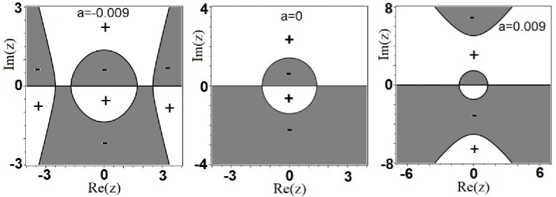
Figure 3: Sign charts of $\mathrm{Im}(\Theta(z;a)$ when $a=-0.009,0,0.009$.

4.1.1 Exponent analysis and steepest descent

Let

$$\Theta(z;a):=z+4az^{3}+2z^{-1}.$$ (4.177)

Then one has

• As $-\frac{1}{96}<a<0$, the function $\Theta(z;a)$ has four different real critical points, namely,

  $$b_{1}(a):=\sqrt{\frac{-1-\sqrt{1+96a}}{24a}},\quad-b_{1}(a),\quad b(a):=\sqrt{\frac{-1+\sqrt{1+96a}}{24a}},\quad-b(a).$$ (4.178)

• As $a=0$, the function $\Theta(z;a)$ has double simple real critical points, namely,

  $$b(a):=\sqrt{2},\qquad-b(a);$$ (4.179)

• As $0<a<\frac{1}{32}$, the function $\Theta(z;a)$ has double simple real critical points, namely,

  $$b(a):=\sqrt{\frac{-1+\sqrt{1+96a}}{24a}},\qquad-b(a).$$ (4.180)

  Moreover, the critical points of $\Theta(z;a)$ are its real roots.

There exists a component of the curve $\mathrm{Im}(\Theta(z;a))=0$ that is a Jordan curve surrounding the origin in the $z$-plane and that passes through two different real critical points, namely, $-b(a)$ and $b(a)$. We select this curve as the jump contour $\Sigma_{2}$ for $Y(z;X,a)$. The real axis divides $\Sigma_{2}$ into an arc $\Sigma_{2}^{+}$ in the upper half-plane and an arc $\Sigma_{2}^{-}$ in the lower half-plane. We introduce thin lens-shaped domains $L^{\pm}$ and $R^{\pm}$ on the left-hand and right-hand sides, respectively, of $\Sigma_{2}^{\pm}$ whose outer boundary arcs $\Sigma_{3}^{\pm}$ and $\Sigma_{4}^{\pm}$ meet the real axis at $\frac{\pi}{4}$ angles as shown in the left-hand panel of Figure 3. The region between $\Sigma_{4}^{\pm}$ and the real axis is denoted $\Omega^{\pm}$. Let the line segment $I:=[-b(a),b(a)]$. Then, we will make the following transformation:

$$W(z;X,a):=Y(z;X,a)\left[\!\!\begin{array}[]{cc}1&0\vskip 3.61371pt\\ e^{2iX^{\frac{1}{2}}\Theta(z;a)}&1\end{array}\!\!\right],\quad z\in L^{+},\vskip 3.61371pt{}$$

$$W(z;X,a):=Y(z;X,a)\left[\!\!\begin{array}[]{cc}\sqrt{2}&\frac{\sqrt{2}}{2}e^{-2iX^{\frac{1}{2}}\Theta(z;a)}\vskip 3.61371pt\\ 0&\frac{\sqrt{2}}{2}\end{array}\!\!\right],\quad z\in R^{+},\vskip 3.61371pt{}$$

$$W(z;X,a):=Y(z;X,a)2^{\frac{\sigma_{3}}{2}},\quad z\in\Omega^{+},\vskip 3.61371pt{}$$

$$W(z;X,a):=Y(z;X,a)2^{-\frac{\sigma_{3}}{2}},\quad z\in\Omega^{-},\vskip 3.61371pt$$

$$W(z;X,a):=Y(z;X,a)\left[\!\!\begin{array}[]{cc}\frac{\sqrt{2}}{2}&0\vskip 3.61371pt\\ -\frac{\sqrt{2}}{2}e^{2iX^{\frac{1}{2}}\Theta(z;a)}&\sqrt{2}\end{array}\!\!\right],\quad z\in R^{-},\vskip 3.61371pt{}$$

$$W(z;X,a):=Y(z;X,a)\left[\!\!\begin{array}[]{cc}1&-e^{-2iX^{\frac{1}{2}}\Theta(z;a)}\vskip 3.61371pt\\ 0&1\end{array}\!\!\right],\quad z\in L^{-},\vskip 3.61371pt{}$$

$$W(z;X,a):=Y(z;X,a),\quad\mathrm{otherwise}.{}$$

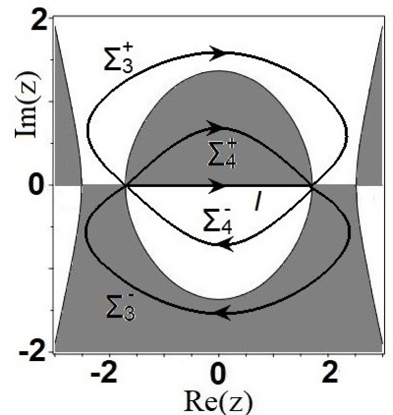
Figure 4: The jump contour $\Sigma_{2}=\Sigma_{2}^{+}\cup\Sigma_{2}^{-}$ for $Y(z;X,a)$ and the regions $L^{\pm},R^{\pm}$ and $\Omega^{\pm}$.

We can easily obtain that $W(z;X,a)$ has no jump on arc $\Sigma_{2}$, namely, $W_{+}(z;X,a)=W_{-}(z;X,a),\quad z\in\Sigma_{2}$. Below we give the jump properties of $W(z;X,a)$ on arcs $\Sigma_{3},\Sigma_{4}$ and line segment $I$.

$$W_{+}(z;X,a)=W_{-}(z;X,a)\left[\!\!\begin{array}[]{cc}1&0\vskip 3.61371pt\\ -e^{2iX^{\frac{1}{2}}\Theta(z;a)}&1\end{array}\!\!\right],\quad z\in\Sigma_{3}^{+},\vskip 3.61371pt{}$$ (4.196)

$$W_{+}(z;X,a)=W_{-}(z;X,a)\left[\!\!\begin{array}[]{cc}1&\frac{1}{2}e^{-2iX^{\frac{1}{2}}\Theta(z;a)}\vskip 3.61371pt\\ 0&1\end{array}\!\!\right],\quad z\in\Sigma_{4}^{+},\vskip 3.61371pt{}$$ (4.199)

$$W_{+}(z;X,a)=W_{-}z;X,a)2^{\sigma_{3}},\qquad\qquad\qquad\qquad\qquad z\in I,\vskip 3.61371pt$$ (4.200)

$$W_{+}(z;X,a)=W_{-}(z;X,a)\left[\!\!\begin{array}[]{cc}1&0\vskip 3.61371pt\\ -\frac{1}{2}e^{2iX^{\frac{1}{2}}\Theta(z;a)}&1\end{array}\!\!\right],\quad z\in\Sigma_{4}^{-},\vskip 3.61371pt{}$$ (4.203)

$$W_{+}(z;X,a)=W_{-}(z;X,a)\left[\!\!\begin{array}[]{cc}1&e^{-2iX^{\frac{1}{2}}\Theta(z;a)}\vskip 3.61371pt\\ 0&1\end{array}\!\!\right],\quad z\in\Sigma_{3}^{-}.{}$$ (4.206)

Since $\mathrm{Im}(\Theta(z;a))>0$ holds on $\Sigma_{3}^{+},\Sigma_{4}^{-}$ while $\mathrm{Im}(\Theta(z;a))<0$ holds on $\Sigma_{3}^{-},\Sigma_{4}^{+}$, the jump matrices are exponentially decreasing on these four contour arcs except near the endpoints $b(a)$ and $-b(a)$. Next, we will find local matrix functions defined near $z=b(a),z=-b(a)$ that exactly satisfy the jump conditions (4.200).

4.1.2 Parametrix construction

Let

$${}\overline{W}^{o}(z;a)=\left(\frac{z+b(a)}{z-b(a)}\right)^{ip\sigma_{3}},\quad z\in\mathbb{C}\setminus I,$$

where $p=\frac{\ln 2}{2\pi}$. Then, we get the jump condition of the function $\overline{W}^{o}(z;a)$ on the line segment $I$:

$${}\overline{W}_{+}^{o}(z;a)=\overline{W}_{-}^{o}(z;a)2^{\sigma_{3}},\quad z\in I.$$

Note that

$${}\Theta^{\prime}(-b(a);a)=\Theta^{\prime}(b(a);a)=0,\qquad\Theta^{\prime\prime}(-b(a);a)<0,\qquad\Theta^{\prime\prime}(b(a);a)>0,$$

we define the following conformal mappings $g_{-b}(z;a)$ and $g_{b}(z;a)$:

$${}\begin{aligned} &g_{-b}(z;a)^{2}=-2\left(\Theta(b(a);a)+\Theta(z;a)\right),\vskip 3.61371pt\\ &g_{b}(z;a)^{2}=2\left(\Theta(z;a)-\Theta(b(a);a)\right)\end{aligned}$$

and we choose the case that $g^{\prime}_{b}(b(a);a)>0$ and $g^{\prime}_{-b}(-b(a);a)<0$. Let $\xi_{-b}:=X^{\frac{1}{4}}g_{-b}(z;a)$ and $\xi_{b}:=X^{\frac{1}{4}}g_{b}(z;a)$. Then the jump conditions are satisfied by

$${}U^{-b}:=iW(z;X,a)e^{iX^{\frac{1}{2}}\Theta(b(a);a)\sigma_{3}}\sigma_{2},\quad~\mathrm{near}~z=-b$$

and by

$${}U^{b}:=W(z;X,a)e^{-iX^{\frac{1}{2}}\Theta(b(a);a)\sigma_{3}}\quad~\mathrm{near}~z=b.$$

Below we give the jump properties of $U^{-b}$ and $U^{b}$:

$$U^{b}_{+}=U^{b}_{-}\left[\!\!\begin{array}[]{cc}1&0\vskip 3.61371pt\\ e^{i\xi_{b}^{2}}&1\end{array}\!\!\right],\quad z\in\Sigma_{3}^{+}\,(\mathrm{away~from}~b(a))\vskip 3.61371pt{}$$ (4.209)

$$U^{b}_{+}=U^{b}_{-}\left[\!\!\begin{array}[]{cc}1&\frac{1}{2}e^{-i\xi_{b}^{2}}\vskip 3.61371pt\\ 0&1\end{array}\!\!\right],\quad z\in\Sigma_{4}^{+}\,(\mathrm{toward}~b(a))\vskip 3.61371pt{}$$ (4.212)

$$U^{b}_{+}=U^{b}_{-}2^{\sigma_{3}},\qquad\qquad\qquad z\in I\,(\mathrm{toward}~b(a))\vskip 3.61371pt{}$$

$$U^{b}_{+}=U^{b}_{-}\left[\!\!\begin{array}[]{cc}1&0\vskip 3.61371pt\\ \frac{1}{2}e^{i\xi_{b}^{2}}&1\end{array}\!\!\right],\quad z\in\Sigma_{4}^{-}\,(\mathrm{toward}~b(a))\vskip 3.61371pt$$ (4.215)

$$U^{b}_{+}=U^{b}_{-}\left[\!\!\begin{array}[]{cc}1&e^{-i\xi_{b}^{2}}\vskip 3.61371pt\\ 0&1\end{array}\!\!\right],\quad z\in\Sigma_{3}^{-}\,(\mathrm{away~from}~b(a)).{}$$ (4.218)

and

$$\begin{aligned} &U^{-b}_{+}=U^{-b}_{-}\left[\!\!\begin{array}[]{cc}1&e^{-i\xi_{-b}^{2}}\vskip 3.61371pt\\ 0&1\end{array}\!\!\right],\quad z\in\Sigma_{3}^{+}\,(\mathrm{away~from}-b(a))\vskip 3.61371pt\\ &U^{-b}_{+}=U^{-b}_{-}\left[\!\!\begin{array}[]{cc}1&0\vskip 3.61371pt\\ \frac{1}{2}e^{i\xi_{-b}^{2}}&1\end{array}\!\!\right],\quad z\in\Sigma_{4}^{+}\,(\mathrm{toward}-b(a))\vskip 3.61371pt\\ &U^{b}_{+}=U^{b}_{-}2^{\sigma_{3}},\qquad\qquad\qquad z\in I\,(\mathrm{toward}-b(a))\vskip 3.61371pt\\ &U^{-b}_{+}=U^{-b}_{-}\left[\!\!\begin{array}[]{cc}1&0\vskip 3.61371pt\\ e^{i\xi_{-b}^{2}}&1\end{array}\!\!\right],\quad z\in\Sigma_{3}^{-}\,(\mathrm{away~from}-b(a))\vskip 3.61371pt\\ &U^{-b}_{+}=U^{-b}_{-}\left[\!\!\begin{array}[]{cc}1&\frac{1}{2}e^{-i\xi_{-b}^{2}}\vskip 3.61371pt\\ 0&1\end{array}\!\!\right],\quad z\in\Sigma_{4}^{-},(\mathrm{toward}-b(a)).\end{aligned}$$ (4.219)

We can normalize the jump matrix near point $-b(a)$ and the jump matrix near point $b(a)$ into the jump matrix about $\xi$.

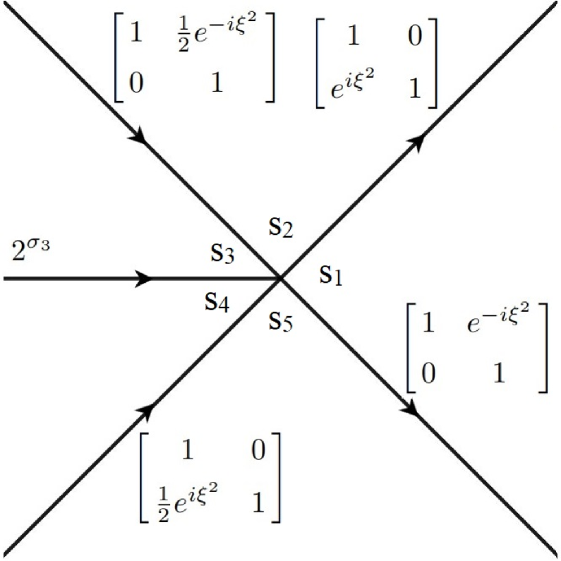
Figure 5: Regional division for $U(\xi)$.

Proposition 4.2.

Riemann-Hilbert Problem 7
Find a $2\times 2$ matrix $U(\xi)$ that satisfies the following properties:

• Analyticity: $U(\xi)$ is analytic for $\xi$ in the five regions shown in Figure 5, namely, $S_{1}:|\mathrm{arg}(\xi)|<\frac{\pi}{4}$, $S_{2}:\frac{\pi}{4}<\mathrm{arg}(\xi)<\frac{3\pi}{4}$, $S_{3}:\frac{3\pi}{4}<\mathrm{arg}(\xi)<\pi$, $S_{4}:-\pi<\mathrm{arg}(\xi)<-\frac{3\pi}{4}$, $S_{5}:-\frac{3\pi}{4}<\mathrm{arg}(\xi)<-\frac{\pi}{4}$ where $-\pi<\mathrm{arg}(\xi)\leq\pi$. It takes continuous boundary values on the excluded rays and at the origin from each sector.

• Jump conditions: The boundary values on the jump contour are related as:

  $$U_{+}(\xi)=U_{-}(\xi)\left[\!\!\begin{array}[]{cc}1&0\vskip 3.61371pt\\ e^{i\xi^{2}}&1\end{array}\!\!\right],\quad\mathrm{arg}(\xi)=\frac{\pi}{4},\vskip 3.61371pt{}$$ (4.222)

  $$U_{+}(\xi)=U_{-}(\xi)\left[\!\!\begin{array}[]{cc}1&\frac{1}{2}e^{-i\xi^{2}}\vskip 3.61371pt\\ 0&1\end{array}\!\!\right],\quad\mathrm{arg}(\xi)=\frac{3\pi}{4},\vskip 3.61371pt{}$$ (4.225)

  $$U_{+}(\xi)=U_{-}(\xi)2^{\sigma_{3}},\qquad\qquad\quad\mathrm{arg}(\xi)=\pi,\vskip 3.61371pt$$ (4.226)

  $$U_{+}(\xi)=U_{-}(\xi)\left[\!\!\begin{array}[]{cc}1&0\vskip 3.61371pt\\ \frac{1}{2}e^{i\xi^{2}}&1\end{array}\!\!\right],\quad\mathrm{arg}(\xi)=-\frac{3\pi}{4},\vskip 3.61371pt{}$$ (4.229)

  $$U_{+}(\xi)=U_{-}(\xi)\left[\!\!\begin{array}[]{cc}1&e^{-i\xi^{2}}\vskip 3.61371pt\\ 0&1\end{array}\!\!\right],\quad\mathrm{arg}(\xi)=-\frac{\pi}{4}.{}$$ (4.232)

• Normalization: $U(\xi)\xi^{ip\sigma_{3}}$ tends to identity matrix as $\xi\rightarrow\infty$, where $p=\frac{\ln(2)}{2\pi}$.

The solution of the Riemann-Hilbert Problem 7 can be expressed explicitly according to the parabolic cylinder function. In particular, the solution satisfies:

$$U(\xi)\xi^{ip\sigma_{3}}=\mathbb{I}+\frac{1}{2i\xi}\left[\!\!\begin{array}[]{cc}0&\gamma\vskip 3.61371pt\\ \gamma^{*}&0\end{array}\!\!\right]+\mathcal{O}(\xi^{-2}),\quad\xi\rightarrow\infty,$$ (4.235)

where

$${}\gamma=\dfrac{2^{\frac{5}{4}}\pi^{\frac{1}{2}}e^{\frac{i\pi}{4}}e^{\frac{i(\ln(2))^{2}}{2\pi}}}{\Gamma(\frac{i\ln(2)}{2\pi})},\quad|\gamma|=\sqrt{2p}.$$

Let

$$\begin{aligned} &T^{-b}(z;a):=i(b-z)^{-ip\sigma_{3}}\left(-\frac{b+z}{g_{-b}(z;a)}\right)^{ip\sigma_{3}}\sigma_{2},\vskip 3.61371pt\\ &T^{b}(z;a):=(b+z)^{ip\sigma_{3}}\left(\frac{g_{b}(z;a)}{z-b}\right)^{ip\sigma_{3}}.\end{aligned}$$ (4.236)

According to Proposition 4.2, we can obtain the following local functions:

$$\begin{aligned} \overline{W}^{-b}(z;X,a)=&-iX^{-\frac{ip\sigma_{3}}{4}}e^{iX^{\frac{1}{2}}\Theta(b;a)\sigma_{3}}T^{-b}(z;a)U(X^{\frac{1}{4}}g_{-b}(z;a))\sigma_{2}e^{-iX^{\frac{1}{2}}\Theta(b;a)\sigma_{3}},\quad z\in\delta_{-b}(r),\vskip 3.61371pt\\ \overline{W}^{b}(z;X,a)=&X^{\frac{ip\sigma_{3}}{4}}e^{-iX^{\frac{1}{2}}\Theta(b;a)\sigma_{3}}T^{b}(z;a)U(X^{\frac{1}{4}}g_{b}(z;a))e^{iX^{\frac{1}{2}}\Theta(b;a)\sigma_{3}},\quad z\in\delta_{b}(r),\end{aligned}$$ (4.237)

where $\delta_{-b}(r)$ and $\delta_{b}(r)$ are small circles with $-b(a)$ as the center and $r$ as the radius, and small circles with $b(a)$ as the center and $r$ as the radius, respectively. When $-\frac{1}{96}<a<0$, we define the following piecewise function:

$$\overline{W}(z;X,a):=\begin{cases}\overline{W}^{-b}(z;X,a),\quad z\in\delta_{-b}(r),\vskip 3.61371pt\\ \overline{W}^{b}(z;X,a),\quad z\in\delta_{b}(r),\vskip 3.61371pt\\ \overline{W}^{o}(z;a),\quad z\in\mathbb{C}\setminus(\overline{\delta_{-b}(r)}\cup\overline{\delta_{b}(r)}\cup I).\end{cases}$$ (4.238)

4.1.3 Error analysis

We consider the following error function:

$$E(z;X,a):=W(z;X,a)\overline{W}(z;X,a)^{-1}.$$ (4.239)

Since $W(z;X,a)$ and $\overline{W}(z;X,a)$ have the same jump property on the line segment $I$, $E(z;X,a)$ has no jump across $I$. Error function $E(z;X,a)$ is analytic in $\mathbb{C}\setminus\Sigma_{5}$ and takes continuous boundary values on $\Sigma_{5}$, where $\Sigma_{5}=\left(\Sigma_{3}^{\pm}\cup\Sigma_{4}^{\pm}\cup\partial\delta_{-b}(r)\cup\partial\delta_{b}(r)\right)\cap\complement_{\mathbb{C}}{(\delta_{-b}(r)\cup\delta_{b}(r))}$. Assuming clockwise orientation of $\delta_{-b}(r)$ and $\delta_{b}(r)$, the boundary values on the jump contour $\Sigma_{5}$ are related as:

$${}E_{+}(z;X,a):=E_{-}(z;X,a)V^{E}(z;X,a).$$

Next, we will analyze the error factors of $V^{E}(z;X,a)$ on each arcs of $\Sigma_{5}$.

Proposition 4.3.

The following identity holds:
(I)

$$\sup_{z\in\left(\Sigma_{3}^{\pm}\cup\Sigma_{4}^{\pm}\right)\cap\complement_{\mathbb{C}}{(\overline{\delta_{-b}(r)}\cup\overline{\delta_{b}(r)})}}||V^{E}(z;X,a)-\mathbb{I}||=\mathcal{O}(e^{-C(a)X^{\frac{1}{2}}}),\quad X\rightarrow+\infty.$$ (4.240)

where $C(a)$ is a constant about $a$ and $||\cdot||$ denotes the matrix norm.

(II)

$$\sup_{z\in\partial\delta_{-b}(r)\cup\partial\delta_{b}(r)}||V^{E}(z;X,a)-\mathbb{I}||=\mathcal{O}(X^{-\frac{1}{4}}),\quad X\rightarrow+\infty.$$ (4.241)

Proof.

When $z\in\left(\Sigma_{3}^{\pm}\cup\Sigma_{4}^{\pm}\right)\cap\complement_{\mathbb{C}}{(\overline{\delta_{-b}(r)}\cup\overline{\delta_{b}(r)})}$, the error term depends on the jump matrix of Eqs. (4.200), then we get formula (I). Note that

$$\begin{aligned} \overline{W}^{-b}(z;X,a)\overline{W}^{o}(z;a)^{-1}=&X^{-\frac{ip\sigma_{3}}{4}}e^{iX^{\frac{1}{2}}\Theta(b(a);a)\sigma_{3}}T^{-b}(z;a)U(\xi_{-b})\vskip 3.61371pt\\ &\times\xi_{-b}^{ip\sigma_{3}}T^{-b}(z;a)^{-1}e^{-iX^{\frac{1}{2}}\Theta(b(a);a)\sigma_{3}}X^{\frac{ip\sigma_{3}}{4}},\quad z\in\partial\delta_{-b}(r),\vskip 3.61371pt\\ \overline{W}^{b}(z;X,a)\overline{W}^{o}(z;a)^{-1}=&X^{\frac{ip\sigma_{3}}{4}}e^{-iX^{\frac{1}{2}}\Theta(b(a),a)\sigma_{3}}T^{b}(z;a)U(\xi_{b})\vskip 3.61371pt\\ &\times\xi_{b}^{ip\sigma_{3}}T^{b}(z;a)^{-1}e^{iX^{\frac{1}{2}}\Theta(b(a);a)\sigma_{3}}X^{-\frac{ip\sigma_{3}}{4}},\quad z\in\partial\delta_{b}(r).\end{aligned}$$ (4.242)

When $z\in\partial\delta_{-b}(r)\cup\partial\delta_{b}(r)$, the error term depends on $U(\xi_{-b})\xi_{-b}^{ip\sigma_{3}}$ and $U(\xi_{b})\xi_{b}^{ip\sigma_{3}}$. According to Eq. (4.235), we get formula (II). Thus the proof is completed.

∎

Using Plemelj formula, we have

$$E(z;X,a)=\mathbb{I}+\frac{1}{2\pi i}\int_{\Sigma_{5}}\dfrac{E_{-}(v;X,a)(V^{E}(v;X,a)-\mathbb{I})}{v-z}dv,\quad z\in\mathbb{C}\setminus\Sigma_{5}.$$ (4.243)

According to Proposition 4.3 and Eq. (4.243), we have

$$E_{-}(z;X,a)-\mathbb{I}=\mathcal{O}(X^{-\frac{1}{4}}),\quad X\rightarrow+\infty.$$ (4.244)

We can get the following Laurent expansion of $E(z;X,a)$ convergent for sufficiently large $|z|$:

$$E(z;X,a)=\mathbb{I}-\frac{1}{2\pi i}\sum_{j=1}^{\infty}z^{-j}\int_{\Sigma_{5}}E_{-}(v;X,a)(V^{E}(v;X,a)-\mathbb{I})v^{j-1}dv.$$ (4.245)

Substituting Eq. (4.239) into Eq. (4.176), we have

$$\widehat{q}^{+}(X,aX^{2})=2iX^{-\frac{1}{2}}\lim_{z\rightarrow\infty}zE_{12}(z;X,a),\quad X>0.$$ (4.246)

Substituting Eq. (4.245) into Eq. (4.246), we have

$$\widehat{q}^{+}(X,aX^{2})=-\frac{1}{\pi X^{\frac{1}{2}}}\int_{\Sigma_{5}}E_{11-}(v;X,a)V^{E}_{12}(v;X,a)+E_{12-}(v;X,a)(V^{E}_{22}(v;X,a)-1)dv.$$ (4.247)

According to Eq. (4.244), we have

$$q^{+}(X,aX^{2})=-\frac{1}{\pi X^{\frac{1}{2}}}\int_{\Sigma_{5}}V^{E}_{12}(v;X,a)dv+\mathcal{O}(X^{-1}),\quad X\rightarrow+\infty.$$ (4.248)

Using Eqs. (4.235) and (4.242), we can obtain the asymptotic expression of $V^{E}_{12}(z;X,a)$:

$$\begin{aligned} &V^{E}_{12}(z;X,a)=\dfrac{X^{-\frac{ip}{2}}e^{2iX^{\frac{1}{2}}\Theta(b;a)}(\gamma T^{-b}_{11}(z;a)^{2}-\gamma^{*}T^{-b}_{12}(z;a)^{2})}{2iX^{\frac{1}{4}}g_{-b}(z;a)}+\mathcal{O}(X^{-\frac{1}{2}}),\quad z\in\partial\delta_{-b}(r),\vskip 3.61371pt\\ &V^{E}_{12}(z;X,a)=\dfrac{X^{\frac{ip}{2}}e^{-2iX^{\frac{1}{2}}\Theta(b;a)}(\gamma T^{b}_{11}(z;a)^{2}-\gamma^{*}T^{b}_{12}(z;a)^{2})}{2iX^{\frac{1}{4}}g_{b}(z;a)}+\mathcal{O}(X^{-\frac{1}{2}}),\quad z\in\partial\delta_{b}(r).\end{aligned}$$ (4.249)

According to above analysis, we can provide the proof of Proposition 1.5.

Proof.

Note that $g_{-b}^{{}^{\prime}}(-b(a);a)=-g_{b}^{{}^{\prime}}(b(a);a)=-\sqrt{24ab+4b^{-3}}$. Substituting Eq. (4.249) into Eq. (4.248), we have

$$\begin{aligned} \widehat{q}^{+}(X,aX^{2})=&\frac{1}{\sqrt{24ab+4b^{-3}}X^{\frac{3}{4}}}\bigg{(}X^{\frac{ip}{2}}e^{-2iX^{\frac{1}{2}}\Theta(b;a)}(\gamma T^{b}_{11}(b(a);a)^{2}-\gamma^{*}T^{b}_{12}(b(a);a)^{2})\vskip 3.61371pt\\ &-X^{-\frac{ip}{2}}e^{2iX^{\frac{1}{2}}\Theta(b;a)}(\gamma T^{-b}_{11}(-b(a);a)^{2}-\gamma^{*}T^{-b}_{12}(-b(a);a)^{2}\bigg{)}+\mathcal{O}(X^{-1}),\quad X\rightarrow+\infty.\end{aligned}$$ (4.250)

According to Eq. (4.236), we have

$$\begin{aligned} &T^{-b}(-b(a);a)=i(2b\sqrt{24ab+4b^{-3}})^{-ip\sigma_{3}}\sigma_{2},\vskip 3.61371pt\\ &T^{b}(b(a);a)=(2b\sqrt{24ab+4b^{-3}})^{ip\sigma_{3}}.\end{aligned}$$ (4.251)

Therefore,

$$\begin{aligned} \widehat{q}^{+}(X,aX^{2})=&\frac{1}{\sqrt{24ab+4b^{-3}}X^{\frac{3}{4}}}\bigg{(}X^{\frac{ip}{2}}e^{-2iX^{\frac{1}{2}}\Theta(b;a)}(\gamma T^{b}_{11}(b(a);a)^{2}-\gamma^{*}T^{b}_{12}(b(a);a)^{2})\vskip 3.61371pt\\ &-X^{-\frac{ip}{2}}e^{2iX^{\frac{1}{2}}\Theta(b;a)}(\gamma T^{-b}_{11}(-b(a);a)^{2}-\gamma^{*}T^{-b}_{12}(-b(a);a)^{2})\bigg{)}+\mathcal{O}(X^{-1})\vskip 3.61371pt\\ =&\frac{1}{\sqrt{24ab+4b^{-3}}X^{\frac{3}{4}}}\bigg{(}X^{\frac{ip}{2}}e^{-2iX^{\frac{1}{2}}\Theta(b;a)}\gamma T^{b}_{11}(b(a);a)^{2}\vskip 3.61371pt\\ &+X^{-\frac{ip}{2}}e^{2iX^{\frac{1}{2}}\Theta(b;a)}\gamma^{*}T^{-b}_{12}(-b(a);a)^{2}\bigg{)}+\mathcal{O}(X^{-1})\vskip 3.61371pt\\ =&\frac{\sqrt{2p}}{\sqrt{24ab+4b^{-3}}X^{\frac{3}{4}}}\bigg{(}X^{\frac{ip}{2}}e^{-2iX^{\frac{1}{2}}\Theta(b;a)}e^{i\mathrm{arg}(\gamma)}(2b\sqrt{24ab+4b^{-3}})^{2ip}\vskip 3.61371pt\\ &+X^{-\frac{ip}{2}}e^{2iX^{\frac{1}{2}}\Theta(b;a)}e^{-i\mathrm{arg}(\gamma)}(2b\sqrt{24ab+4b^{-3}})^{-2ip}\bigg{)}+\mathcal{O}(X^{-1})\vskip 3.61371pt\\ =&\frac{\sqrt{2p}\cos(\phi(X,a))}{X^{\frac{3}{4}}\sqrt{6ab+b^{-3}}}+\mathcal{O}(X^{-1}),\quad X\rightarrow+\infty.\end{aligned}$$ (4.252)

Thus the proof is completed. ∎

Corollary 4.1.

Let $a=0$ and $\Theta(z;a):=z+2z^{-1}$. Then as $X\rightarrow+\infty$, we have

$$\begin{aligned} \widehat{q}^{+}(X,0)=&\frac{2^{\frac{3}{4}}\sqrt{\ln 2}}{\sqrt{\pi}X^{\frac{3}{4}}}\cos\bigg{(}2^{\frac{5}{2}}X^{\frac{1}{2}}-\frac{\ln 2}{4\pi}\ln(X)+\mathrm{arg}\left(\Gamma\left(\frac{i\ln 2}{2\pi}\right)\right)-\frac{9(\ln 2)^{2}}{4\pi}-\frac{\pi}{4}\bigg{)}+\mathcal{O}(X^{-1}).\end{aligned}$$ (4.253)

Proof.

When $a=0$, the critical points $b(0)=\sqrt{2}$. Using Theorem 1.5, we obtain Eq. (4.253). Thus the proof is completed. ∎

4.2 Asymptotic behavior of $\widehat{q}^{\pm}(X,T)$ for large $T$: part results

We will study the asymptotic behavior of $\widehat{q}^{\pm}(X,T)$ when $T$ is large. To this end, let us make the following transforms:

$$T:=\sigma|T|,\quad X:=w|T|^{\frac{1}{2}},\quad\Lambda:=|T|^{-\frac{1}{4}}z.$$ (4.254)

The phase conjugating the jump matrix for $D^{\pm}(\Lambda;X,T)$ can be rewritten as

$$\Lambda X+4\Lambda^{3}T\pm 2\Lambda^{-1}=|T|^{\frac{1}{4}}(4\sigma z^{3}+wz\pm 2z^{-1}).$$ (4.255)

Similarly to the asymptotic behavior for large $X$, we only need to consider the case that $|T|^{\frac{1}{4}}(4z^{3}+wz+2z^{-1})$. Setting

$$Y(z;T,w):=D^{+}(T^{-\frac{1}{4}}z;wT^{\frac{1}{2}},T),\quad T>0.$$ (4.256)

Using Eq. (3.108), we have

$$\widehat{q}^{+}(wT^{\frac{1}{2}},T)=2iT^{-\frac{1}{4}}\lim_{z\rightarrow\infty}zY_{12}(z;T,w),\quad T>0.$$ (4.257)

Let $\Sigma_{2}$ be an arbitrary Jordan curve surrounding $z=0$. Assuming clockwise orientation of $\Sigma_{2}$, the boundary values on the jump contour $\Sigma_{2}$ are related as:

$$Y_{+}(z;T,w)=Y_{-}(z;T,w)e^{-iT^{\frac{1}{4}}\theta(z;w)\sigma_{3}}Q^{-1}e^{iT^{\frac{1}{4}}\theta(z;w)\sigma_{3}},\quad z\in\Sigma_{2}.$$ (4.258)

where $\theta(z;w)=4z^{3}+wz+2z^{-1}$. When $|w|>\sqrt{32}$, the function $\theta(z;w)$ has double simple real roots. This case is equivalent to the case which two simple real root in the asymptotic behavior for large $X$. When $0<|w|<\sqrt{32}$, the function $\theta(z;a)$ has double simple real roots, namely, $\sqrt{\frac{-w+\sqrt{w^{2}+96}}{24}}$ and $-\sqrt{\frac{-w+\sqrt{w^{2}+96}}{24}}$. When $w=0$, the function $\Theta(z;a)$ has double simple real roots, namely, $6^{-\frac{1}{4}}$ and $-6^{-\frac{1}{4}}$. When $w=0$ and $w=2$, the sign chart of $\theta(z;w)$ are illustrated in Figure 6.

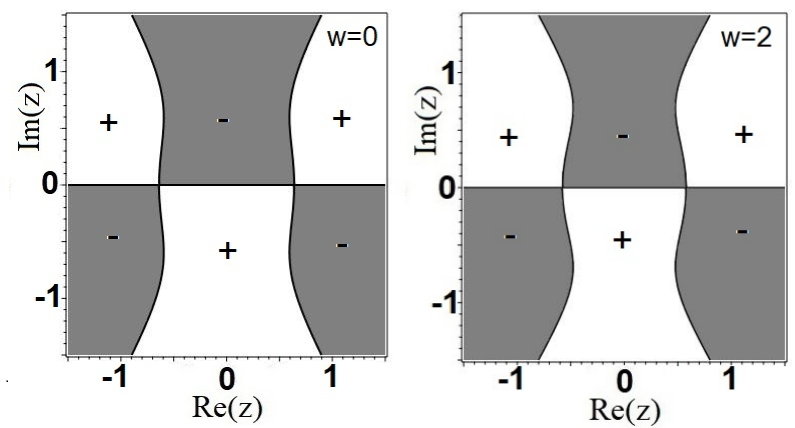
Figure 6: Sign charts of $\theta(z;w)$ when $w=0,2$.

4.2.1 The $g$-function

Suppose that $g(z;w)$ is a scalar function, that satisfies $g(z;w)=\mathcal{O}(\frac{1}{z})$ as $z\rightarrow\infty$, and the boundary values on the jump contour are related as:

$$g_{+}(z;w)+g_{-}(z;w)+2\theta(z;w)=\mathrm{constant}.$$ (4.259)

It is easy to check that the function $(g_{z}(z;w)+\theta_{z}(z;w))^{2}$ is analytic for $z\in\mathbb{C}\setminus\!\{0\}$. Then we can obtain the asymptotic expression of the function $(g_{z}(z;w)+\theta_{z}(z;w))^{2}$ at $z=0$ and $z=\infty$:

$$\begin{aligned} &(g_{z}(z;w)+\theta_{z}(z;w))^{2}=4z^{-4},\quad z\rightarrow 0,\vskip 3.61371pt\\ &(g_{z}(z;w)+\theta_{z}(z;w))^{2}=144z^{4}+24wz^{2}+\mathcal{O}(1),\quad z\rightarrow\infty.\end{aligned}$$ (4.260)

According to Liouville’s theorem, we can rewrite Eq. (4.260) as

$$\begin{aligned} &(g_{z}(z;w)+\theta_{z}(z;w))^{2}=z^{-4}Q(z;w),\vskip 3.61371pt\\ &Q(z;w)=144z^{8}+24wz^{6}+d_{4}(w)z^{4}+d_{3}(w)z^{3}+d_{2}(w)z^{2}+4.\end{aligned}$$ (4.261)

Here we will be interested in the main case in which $Q(z;w)$ has two double roots and four simple roots:

$$Q(z;w)=144(z^{2}+a_{1}z+a_{0})^{2}(z^{2}+b_{1}z+b_{0})(z^{2}+c_{1}z+c_{0}).$$ (4.262)

Expanding out the right-hand side of Eq. (4.262) and comparing with the coefficients of $z^{7},z^{6},z^{5},z^{1}$ and $z^{0}$, we have

$$\begin{aligned} &288a_{1}+144b_{1}+144c_{1}=0,\vskip 3.61371pt\\ &144a_{1}^{2}+288a_{1}b_{1}+288a_{0}+144b_{0}+144(2a_{1}+b_{1})c_{1}+144c_{0}=24w,\vskip 3.61371pt\\ &288a_{0}a_{1}+144(a_{1}^{2}+2a_{0})b_{1}+288a_{1}b_{0}+144(a_{1}^{2}+2a_{1}b_{1}+2a_{0}+b_{0})c_{1}+144(2a_{1}+b_{1})c_{0}=0,\vskip 3.61371pt\\ &144a_{0}^{2}b_{0}c_{1}+144(a_{0}^{2}b_{1}+2a_{0}a_{1}b_{0})c_{0}=0,\vskip 3.61371pt\\ &144a_{0}^{2}b_{0}c_{0}=4.\end{aligned}$$ (4.263)

To solve the above equation (4.263), we choose a constraint

$${}a_{1}=0,\quad b_{1}=0,\quad c_{1}=0.$$

For convenience, we add constraints on simple zeros of $Q(z;w)$, and the function $Q(z;w)$ can be rewritten as

$$Q(z;w)=144(z^{2}-d_{0}^{2})^{2}(z^{2}-(d_{1}+id_{2})^{2})(z^{2}-(d_{1}-id_{2})^{2}).$$ (4.264)

Expanding out the right-hand side of Eq. (4.264) and comparing with the coefficients of $z^{6}$ and $z^{0}$, we have

$$\begin{aligned} &-288d_{0}^{2}-288d_{1}^{2}+288d_{2}^{2}=24w,\vskip 3.61371pt\\ &144d_{0}^{4}d_{1}^{4}+288d_{0}^{4}d_{1}^{2}d_{2}^{2}+144d_{0}^{4}d_{2}^{4}=4.\end{aligned}$$ (4.265)

Note that the following two constraints must be met:

$$\begin{aligned} &144d_{0}^{4}+(576d_{1}^{2}-576d_{2}^{2})d_{0}^{2}+144(d_{1}^{2}+d_{2}^{2})^{2}=w^{2}+24(\lim_{z=\infty}z^{2}g_{z}(z;w)-2),\vskip 3.61371pt\\ &-288((d_{1}^{2}-d_{2}^{2})d_{0}^{2}+(d_{1}^{2}+d_{2}^{2})^{2})d_{0}^{2}=2w(\lim_{z=\infty}z^{2}g_{z}(z;w)-2).\end{aligned}$$ (4.266)

By solving Eqs. (4.265) and (4.266), we obtain

$${}d_{0}=\frac{1}{12}\sqrt{6\sqrt{w^{2}+96}-6w},\quad d_{1}=0,\quad d_{2}=\frac{1}{2d_{0}}\sqrt{\frac{12d_{0}^{4}+d_{0}^{2}w+2}{6}}.$$

Specifically, when $w=0$, we have

$${}d_{0}=6^{-\frac{1}{4}},\quad d_{1}=0,\quad d_{2}=6^{-\frac{1}{4}}.$$

Then, the function $Q(z;w)$ has the following four double roots: $d_{0}(w),~-d_{0}(w),~id_{2}(w),~-id_{2}(w).$

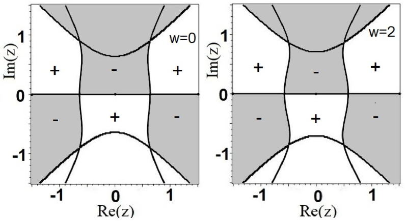
Figure 7: Sign charts of $h(z;w)$ when $w=0,2$.

4.2.2 Exponent analysis and steepest descent

Let $h(z;w)=g(z;w)+\theta(z;w)$. For convenience, we denote $b(w):=|d_{0}(w)|,d(w):=id_{2}(w)$. There exists a component of the curve $\mathrm{Im}(h(z;a))=0$ that is a Jordan curve surrounding the origin in the $z$-plane and that passes through two real simple critical points, namely, $-b(w)$ and $b(w)$. We select this curve as the jump contour $\Sigma_{2}$ for $Y(z;T,w)$. The real axis divides $\Sigma_{2}$ into an arc $\Sigma_{2}^{+}$ in the upper half-plane and an arc $\Sigma_{2}^{-}$ in the lower half-plane. We introduce thin lens-shaped domains $L^{\pm}$ and $R^{\pm}$ on the left-hand and right-hand sides, respectively, of $\Sigma_{2}^{\pm}$ whose outer boundary arcs $\Sigma_{3}^{\pm}$ and $\Sigma_{4}^{\pm}$ meet the real axis at $\frac{\pi}{4}$ angles as shown in the left-hand panel of Figure 8. The region between $\Sigma_{4}^{\pm}$ and the real axis is denoted $\Omega^{\pm}$. Let the line segment $I:=[-b(w),b(w)]$. Then, we will make the following transformations:

$$W(z;T,w):=Y(z;T,w)\left[\!\!\begin{array}[]{cc}1&0\vskip 3.61371pt\\ e^{2iT^{1/4}\theta(z;w)}&1\end{array}\!\!\right]e^{iT^{1/4}g(z;w)\sigma_{3}},\quad z\in L^{+}_{l,r},\vskip 3.61371pt{}$$ (4.269)

$$W(z;T,w):=Y(z;T,w)\left[\!\!\begin{array}[]{cc}\sqrt{2}&\frac{\sqrt{2}}{2}e^{-2iT^{1/4}\theta(z;w)}\vskip 3.61371pt\\ 0&\frac{\sqrt{2}}{2}\end{array}\!\!\right]e^{iT^{1/4}g(z;w)\sigma_{3}},\quad z\in R^{+}_{l,r},\vskip 3.61371pt{}$$ (4.272)

$$W(z;T,w):=Y(z;T,w)2^{\frac{\sigma_{3}}{2}}e^{iT^{1/4}g(z;w)\sigma_{3}},\quad z\in\Omega^{+},\vskip 3.61371pt{}$$

$$W(z;T,w):=Y(z;T,w)2^{-\frac{\sigma_{3}}{2}}e^{iT^{1/4}g(z;w)\sigma_{3}},\quad z\in\Omega^{-},\vskip 3.61371pt{}$$

$$W(z;T,w):=Y(z;T,w)\left[\!\!\begin{array}[]{cc}\frac{\sqrt{2}}{2}&0\vskip 3.61371pt\\ -\frac{\sqrt{2}}{2}e^{2iT^{1/4}\theta(z;w)}&\sqrt{2}\end{array}\!\!\right]e^{iT^{1/4}g(z;w)\sigma_{3}},\quad z\in R^{-}_{l,r},\vskip 3.61371pt{}$$ (4.275)

$$W(z;T,w):=Y(z;T,w)\left[\!\!\begin{array}[]{cc}1&-e^{-2iT^{1/4}\theta(z;w)}\vskip 3.61371pt\\ 0&1\end{array}\!\!\right]e^{iT^{1/4}g(z;w)\sigma_{3}},\quad z\in L^{-}_{l,r},\vskip 3.61371pt$$ (4.278)

$$W(z;T,w):=Y(z;T,w)2^{\frac{\sigma_{3}}{2}}\left[\!\!\begin{array}[]{cc}1&-\frac{1}{2}e^{-2iT^{1/4}\theta(z;w)}\vskip 3.61371pt\\ 0&1\end{array}\!\!\right]e^{iT^{1/4}g(z;w)\sigma_{3}},\quad z\in R_{1,l}^{+}\cup R_{1,r}^{+},\vskip 3.61371pt{}$$ (4.281)

$$W(z;T,w):=Y(z;T,w)\left[\!\!\begin{array}[]{cc}1&e^{-2iT^{1/4}\theta(z;w)}\vskip 3.61371pt\\ 0&1\end{array}\!\!\right]e^{iT^{1/4}g(z;w)\sigma_{3}},\quad z\in L_{1,l}^{+}\cup L_{1,r}^{+},\vskip 3.61371pt{}$$ (4.284)

$$W(z;T,w):=Y(z;T,w)2^{-\frac{\sigma_{3}}{2}}\left[\!\!\begin{array}[]{cc}1&0\vskip 3.61371pt\\ \frac{1}{2}e^{2iT^{1/4}\theta(z;w)}&1\end{array}\!\!\right]e^{iT^{1/4}g(z;w)\sigma_{3}},\quad z\in R_{1,l}^{-}\cup R_{1,r}^{-},\vskip 3.61371pt{}$$ (4.287)

$$W(z;T,w):=Y(z;T,w)\left[\!\!\begin{array}[]{cc}1&0\vskip 3.61371pt\\ -e^{2iT^{1/4}\theta(z;w)}&1\end{array}\!\!\right]e^{iT^{1/4}g(z;w)\sigma_{3}},\quad z\in L_{1,l}^{-}\cup L_{1,r}^{-},\vskip 3.61371pt{}$$ (4.290)

$$W(z;T,w):=Y(z;T,w)e^{iT^{1/4}g(z;w)\sigma_{3}},\quad\mathrm{otherwise}.{}$$

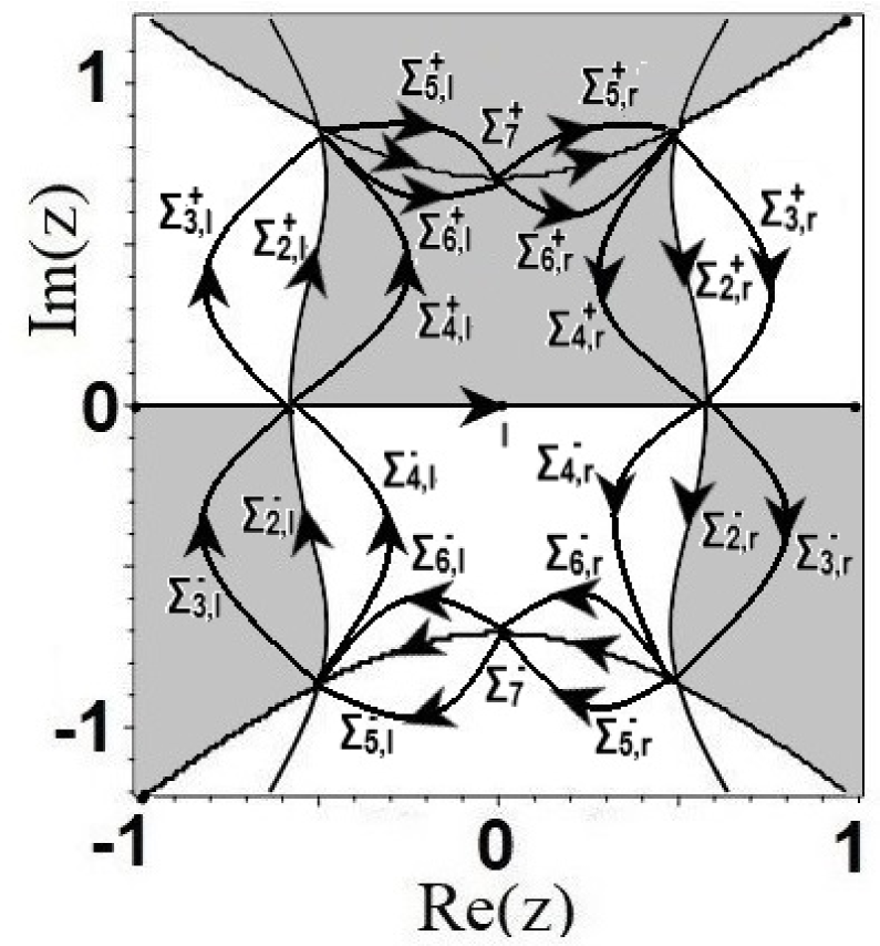
Figure 8: Regional division for large $T$.

We can easily find that $W(z;T,w)$ has no jump on the arc $\Sigma_{2}$, namely, $W_{+}(z;T,w)=W_{-}(z;T,w),\quad z\in\Sigma_{2}$. Below we give the jump properties of $W(z;T,w)$ on the arcs $\Sigma_{j},\,(j=3,4,5,6,7)$ and line segment $I$.

$$W_{+}(z;T,w)=W_{-}(z;T,w)\left[\!\!\begin{array}[]{cc}1&0\vskip 3.61371pt\\ -e^{2iT^{\frac{1}{4}}h(z;w)}&1\end{array}\!\!\right],\quad z\in\Sigma_{3,l,r}^{+},\vskip 3.61371pt{}$$ (4.293)

$$W_{+}(z;T,w)=W_{-}(z;T,w)\left[\!\!\begin{array}[]{cc}1&\frac{1}{2}e^{-2iT^{\frac{1}{4}}h(z;w)}\vskip 3.61371pt\\ 0&1\end{array}\!\!\right],\quad z\in\Sigma_{4,l,r}^{+},\vskip 3.61371pt{}$$ (4.296)

$$W_{+}(z;T,w)=W_{-}(z;T,w)2^{\sigma_{3}},\qquad z\in I,\vskip 3.61371pt{}$$

$$W_{+}(z;T,w)=W_{-}(z;T,w)\left[\!\!\begin{array}[]{cc}1&0\vskip 3.61371pt\\ -\frac{1}{2}e^{2iT^{\frac{1}{4}}h(z;w)}&1\end{array}\!\!\right],\quad z\in\Sigma_{4,l,r}^{-},\vskip 3.61371pt{}$$ (4.299)

$$W_{+}(z;T,w)=W_{-}(z;T,w)\left[\!\!\begin{array}[]{cc}1&e^{-2iT^{\frac{1}{4}}h(z;w)}\vskip 3.61371pt\\ 0&1\end{array}\!\!\right],\quad z\in\Sigma_{3,l,r}^{-},\vskip 3.61371pt$$ (4.302)

$$W_{+}(z;T,w)=W_{-}(z;T,w)\left[\!\!\begin{array}[]{cc}1&-e^{-2iT^{\frac{1}{4}}h(z;w)}\vskip 3.61371pt\\ 0&1\end{array}\!\!\right],\quad z\in\Sigma_{5,l,r}^{+},\vskip 3.61371pt{}$$ (4.305)

$$W_{+}(z;T,w)=W_{-}(z;T,w)\left[\!\!\begin{array}[]{cc}1&-\frac{1}{2}e^{-2iT^{\frac{1}{4}}h(z;w)}\vskip 3.61371pt\\ 0&1\end{array}\!\!\right],\quad z\in\Sigma_{6,l,r}^{+},\vskip 3.61371pt{}$$ (4.308)

$$W_{+}(z;T,w)=W_{-}(z;T,w)\left[\!\!\begin{array}[]{cc}1&0\vskip 3.61371pt\\ \frac{1}{2}e^{2iT^{\frac{1}{4}}h(z;w)}&1\end{array}\!\!\right],\quad z\in\Sigma_{6,l,r}^{-},\vskip 3.61371pt{}$$ (4.311)

$$W_{+}(z;T,w)=W_{-}(z;T,w)\left[\!\!\begin{array}[]{cc}1&0\vskip 3.61371pt\\ e^{2iT^{\frac{1}{4}}h(z;w)}&1\end{array}\!\!\right],\quad z\in\Sigma_{5,l,r}^{-},\vskip 3.61371pt{}$$ (4.314)

$$W_{+}(z;T,w)=W_{-}(z;T,w)\left[\!\!\begin{array}[]{cc}0&e^{-iT^{\frac{1}{4}}c(w)}\vskip 3.61371pt\\ -e^{iT^{\frac{1}{4}}c(w)}&0\end{array}\!\!\right],\quad z\in\Sigma_{7}^{+}\cup\Sigma_{7}^{-},{}$$ (4.317)

where $c(w)=g_{+}(z;w)+g_{-}(z;w)+2\theta(z;w),~z\in\Sigma_{7}^{+}\cup\Sigma_{7}^{-}$. Since $\mathrm{Im}(h(z;w))>0$ holds on $\Sigma_{3,r}^{+},\Sigma_{3,l}^{+},\Sigma_{4,l}^{-},\Sigma_{4,r}^{-},\Sigma_{5,l,r}^{-},\Sigma_{6,l,r}^{-}$ while $\mathrm{Im}(h(z;w))<0$ holds on $\Sigma_{3,l}^{-},\Sigma_{3,r}^{-},\Sigma_{4,l}^{+},\Sigma_{4,r}^{+},\Sigma_{5,l,r}^{+},\Sigma_{6,l,r}^{+}$, the jump matrices are exponentially decreasing on these four contour arcs except near the endpoints $b(w),-b(w),d(w)$ and $-d(w)$. At these four endpoints, the new models are needed, which cannot be provided in this paper now. This will be further studied in our future work.

4.3 Transitional asymptotic behavior: $a\rightarrow-1/96$

Let $\Theta(z;a):=z+4az^{3}+2z^{-1}$. When $a\rightarrow-\frac{1}{96}:=a_{c}$, there is a pair of critical points (real for $-\frac{1}{96}<a<0$ and complex-conjugate for $a<-\frac{1}{96}$) near the double critical point $b_{c}:=2$ and a pair of critical points (real for $-\frac{1}{96}<a<0$ and complex-conjugate for $a<-\frac{1}{96}$) near the double critical point $-b_{c}$. Sign chart of $\Theta(z;a)$ when $a=-\frac{1}{96}$ is shown in Figure 9. Note that $\Theta(b_{c};a_{c}):=\frac{8}{3}$ and $\Theta(-b_{c};a_{c}):=-\frac{8}{3}$. The Taylor expansion of $\Theta(z;a)$ about $z=-b_{c},a=a_{c}$ as:

$$\begin{aligned} \Theta(z;a):=&-\frac{8}{3}-32(a-a_{c})+48(a-a_{c})(z+b_{c})-24(a-a_{c})(z+b_{c})^{2}-\frac{1}{6}(z+b_{c})^{3}\vskip 3.61371pt\\ &+4(a-a_{c})(z+b_{c})^{3}-\frac{1}{16}(z+b_{c})^{4}-\frac{1}{32}(z+b_{c})^{5}+\mathcal{O}((z+b_{c})^{6}),\quad z\rightarrow-b_{c},\end{aligned}$$ (4.318)

and when $a=a_{c}$, we have

$$\begin{aligned} \Theta(z;a_{c}):=&-\frac{8}{3}-\frac{1}{6}(z+b_{c})^{3}-\frac{1}{16}(z+b_{c})^{4}-\frac{1}{32}(z+b_{c})^{5}+\mathcal{O}((z+b_{c})^{6}),\quad z\rightarrow-b_{c}.\end{aligned}$$ (4.319)

Figure 9: Sign charts of $\Theta(z;a)$ when $a=-\frac{1}{96}$.

According to [23], we can define a Schwarz-symmetric conformal mapping $z\mapsto M_{1}(z;a)$ in the neighborhood of $z=-b_{c},a=a_{c}$ by the equation:

$${}2\Theta(z;a)=M_{1}(z;a)^{3}+r_{1}(a)M_{1}(z;a)-s_{1}(a),$$

where $r_{1}(a)$ and $s_{1}(a)$ are real analytic functions of $a$ near $a_{c}$. And they satisfy the following properties:

$$r_{1}(a_{c})=0,\quad s_{1}(a_{c})=\frac{16}{3},\quad M_{1}^{{}^{\prime}}(-b_{c};a_{c})=-3^{-\frac{1}{3}}<0,\quad s_{1}^{{}^{\prime}}(a_{c})=64,\quad r_{1}^{{}^{\prime}}(a_{c})=-96\cdot 3^{\frac{1}{3}}.$$ (4.320)

Moreover, we denote by $z_{1}(a)$ the preimage of $M_{1}(z;a)=0$. It is an analytic function of $a$ that satisfies $z_{1}(a_{c})=-b_{c}$.

On the other hand, the Taylor expansion of $\Theta(z;a)$ about $z=b_{c},a=a_{c}$ as:

$$\begin{aligned} \Theta(z;a):=&\frac{8}{3}+32(a-a_{c})+48(a-a_{c})(z-b_{c})+24(a-a_{c})(z-b_{c})^{2}-\frac{1}{6}(z-b_{c})^{3}\vskip 3.61371pt\\ &+4(a-a_{c})(z-b_{c})^{3}+\frac{1}{16}(z-b_{c})^{4}-\frac{1}{32}(z-b_{c})^{5}+\mathcal{O}((z-b_{c})^{6}),\quad z\rightarrow b_{c},\end{aligned}$$ (4.321)

and when $a=a_{c}$, we have

$$\begin{aligned} \Theta(z;a_{c}):=&\frac{8}{3}-\frac{1}{6}(z-b_{c})^{3}+\frac{1}{16}(z-b_{c})^{4}-\frac{1}{32}(z-b_{c})^{5}+\mathcal{O}((z-b_{c})^{6}),\quad z\rightarrow b_{c}.\end{aligned}$$ (4.322)

Similarly, we can define a Schwarz-symmetric conformal mapping $z\mapsto M_{2}(z;a)$ in the neighborhood of $z=b_{c},a=a_{c}$ by the equation:

$${}-2\Theta(z;a)=M_{2}(z;a)^{3}+r_{2}(a)M_{2}(z;a)-s_{2}(a),$$

where $r_{2}(a)$ and $s_{2}(a)$ are real analytic functions of $a$ near $a_{c}$. And they satisfy the following properties:

$$r_{2}(a_{c})=0,\quad s_{2}(a_{c})=\frac{16}{3},\quad M_{2}^{\prime}(b_{c};a_{c})=3^{-\frac{1}{3}}>0,\quad s_{2}^{\prime}(a_{c})=64,\quad r_{2}^{\prime}(a_{c})=-96\cdot 3^{\frac{1}{3}}.$$ (4.323)

Moreover, we denote by $z_{2}(a)$ the preimage of $M_{2}(z;a)=0$. It is an analytic function of $a$ that satisfies $z_{2}(a_{c})=b_{c}$

4.3.1 Parametrix modification

The matrix function $W(z;X,a)$ and its jumping properties are given by Eqs. (4.200) and (4.1.1). We define the following function:

$${}\overline{W}^{o}(z;a)=\left(\frac{z-z_{1}(a)}{z-z_{2}(a)}\right)^{ip\sigma_{3}},\quad z\in\mathbb{C}\setminus[z_{1}(a),z_{2}(a)],$$

where $p=\frac{\ln(2)}{2\pi}$. Then, we get the jump condition of the function $\overline{W}^{o}(z;a)$ on the line segment $[z_{1}(a),z_{2}(a)]$:

$${}\overline{W}_{+}^{o}(z;a)=\overline{W}_{-}^{o}(z;a)2^{\sigma_{3}},\quad z\in[z_{1}(a),z_{2}(a)].$$

Let $\xi_{-b}:=X^{\frac{1}{6}}M_{1},~y_{1}:=X^{\frac{1}{3}}r_{1}$ and $\xi_{b}:=X^{\frac{1}{6}}M_{2},~y_{2}:=X^{\frac{1}{3}}r_{2}$. Then the jump conditions satisfied by

$${}U^{-b}:=iW(z;X,a)e^{\frac{i}{2}X^{\frac{1}{2}}s_{1}(a)\sigma_{3}}\sigma_{2},\quad~\mathrm{near}~z=-b_{c}$$

and by

$${}U^{b}:=W(z;X,a)e^{-\frac{i}{2}X^{\frac{1}{2}}s_{2}(a)\sigma_{3}}\quad~\mathrm{near}~z=b_{c}.$$

The outer parametrix can also be expressed near $z=-b_{c}$ or $z=b_{c}$ in terms of the relevant conformal coordinate:

$$\begin{aligned} &i\overline{W}^{o}(z;a)e^{\frac{i}{2}X^{\frac{1}{2}}s_{1}(a)\sigma_{3}}\sigma_{2}=X^{-\frac{i}{6}p\sigma_{3}}e^{\frac{i}{2}X^{\frac{1}{2}}s_{1}(a)\sigma_{3}}T^{-b}(z;a)\xi_{-b}^{-ip\sigma_{3}},\vskip 3.61371pt\\ &\overline{W}^{o}(z;a)e^{-\frac{i}{2}X^{\frac{1}{2}}s_{2}(a)\sigma_{3}}=X^{\frac{i}{6}p\sigma_{3}}e^{-\frac{i}{2}X^{\frac{1}{2}}s_{2}(a)\sigma_{3}}T^{b}(z;a)\xi_{b}^{-ip\sigma_{3}},\end{aligned}$$ (4.324)

where

$$\begin{aligned} &T^{-b}(z;a):=i(z_{2}(a)-z)^{-ip\sigma_{3}}\left(\frac{z_{1}(a)-z}{M_{1}(z;a)}\right)^{ip\sigma_{3}}\sigma_{2},\vskip 3.61371pt\\ &T^{b}(z;a):=(z-z_{1}(a))^{ip\sigma_{3}}\left(\frac{M_{2}(z;a)}{z-z_{2}(a)}\right)^{ip\sigma_{3}}.\end{aligned}$$ (4.325)

Below we give the jump properties of $U^{-b}$ and $U^{b}$:

$$\begin{aligned} &U^{b}_{+}=U^{b}_{-}\left[\!\!\begin{array}[]{cc}1&0\vskip 3.61371pt\\ e^{-i(\xi_{b}^{3}+y_{2}\xi_{b})}&1\end{array}\!\!\right],\quad z\in\Sigma_{3}^{+}\,(\mathrm{away~from}~z_{2}(a)),\vskip 5.78172pt\\ &U^{b}_{+}=U^{b}_{-}\left[\!\!\begin{array}[]{cc}1&\frac{1}{2}e^{i(\xi_{b}^{3}+y_{2}\xi_{b})}\vskip 5.78172pt\\ 0&1\end{array}\!\!\right],\quad z\in\Sigma_{4}^{+}\,(\mathrm{toward}~z_{2}(a)),\vskip 5.78172pt\\ &U^{b}_{+}=U^{b}_{-}2^{\sigma_{3}},\qquad\qquad\qquad\qquad z\in I\,(\mathrm{toward}~z_{2}(a)),\vskip 5.78172pt\\ &U^{b}_{+}=U^{b}_{-}\left[\!\!\begin{array}[]{cc}1&0\vskip 5.78172pt\\ \frac{1}{2}e^{-i(\xi_{b}^{3}+y_{2}\xi_{b})}&1\end{array}\!\!\right],\quad z\in\Sigma_{4}^{-}\,(\mathrm{toward}~z_{2}(a)),\vskip 5.78172pt\\ &U^{b}_{+}=U^{b}_{-}\left[\!\!\begin{array}[]{cc}1&e^{i(\xi_{b}^{3}+y_{2}\xi_{b})}\vskip 3.61371pt\\ 0&1\end{array}\!\!\right],\qquad z\in\Sigma_{3}^{-}\,(\mathrm{away~from}~z_{2}(a)).\end{aligned}$$ (4.326)

and

$$\begin{aligned} &U^{-b}_{+}=U^{-b}_{-}\left[\!\!\begin{array}[]{cc}1&e^{i(\xi_{-b}^{3}+y_{1}\xi_{-b})}\vskip 3.61371pt\\ 0&1\end{array}\!\!\right],\quad z\in\Sigma_{3}^{+},(\mathrm{away~from}z_{1}(a))\vskip 3.61371pt\\ &U^{-b}_{+}=U^{-b}_{-}\left[\!\!\begin{array}[]{cc}1&0\vskip 3.61371pt\\ \frac{1}{2}e^{-i(\xi_{-b}^{3}+y_{1}\xi_{-b})}&1\end{array}\!\!\right],\quad z\in\Sigma_{4}^{+}\,(\mathrm{toward}~z_{1}(a)),\vskip 3.61371pt\\ &U^{b}_{+}=U^{b}_{-}2^{\sigma_{3}},\qquad\qquad\qquad\qquad\qquad z\in I\,(\mathrm{toward}~z_{1}(a)),\vskip 3.61371pt\\ &U^{-b}_{+}=U^{-b}_{-}\left[\!\!\begin{array}[]{cc}1&0\vskip 3.61371pt\\ e^{-i(\xi_{-b}^{3}+y_{1}\xi_{-b})}&1\end{array}\!\!\right],\quad z\in\Sigma_{3}^{-}\,(\mathrm{away~from}~z_{1}(a)),\vskip 3.61371pt\\ &U^{-b}_{+}=U^{-b}_{-}\left[\!\!\begin{array}[]{cc}1&\frac{1}{2}e^{i(\xi_{-b}^{3}+y_{1}\xi_{-b})}\vskip 3.61371pt\\ 0&1\end{array}\!\!\right],\quad z\in\Sigma_{4}^{-}\,(\mathrm{toward}~z_{1}(a)).\end{aligned}$$ (4.327)

We can normalize the jump matrix near point $z_{1}(a)$ and the jump matrix near point $z_{2}(a)$ into the jump matrix about $\xi$.

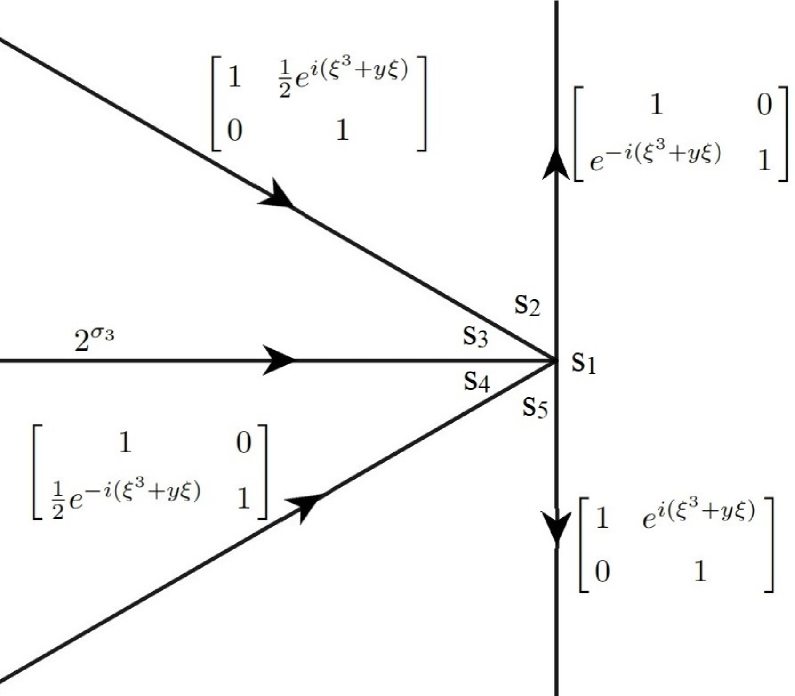
Figure 10: Regional division for $U(\xi)$.

Proposition 4.4.

Riemann-Hilbert Problem 8

Find a $2\times 2$ matrix $U(\xi;y)$ that satisfies the following properties:

• Analyticity: $U(\xi;y)$ is analytic for $\xi$ in the five regions shown in Figure 10, namely, $S_{1}:|\mathrm{arg}(\xi)|<\frac{\pi}{2}$, $S_{2}:\frac{\pi}{2}<\mathrm{arg}(\xi)<\frac{5\pi}{6}$, $S_{3}:\frac{5\pi}{6}<\mathrm{arg}(\xi)<\pi$, $S_{4}:-\pi<\mathrm{arg}(\xi)<-\frac{5\pi}{6}$, $S_{5}:-\frac{5\pi}{6}<\mathrm{arg}(\xi)<-\frac{\pi}{2}$ where $-\pi<\mathrm{arg}(\xi)\leq\pi$. It takes continuous boundary values on the excluded rays and at the origin from each sector.

• Jump conditions: The boundary values on the jump contour are related as:

  $$\begin{aligned} &U_{+}(\xi;y)=U_{-}(\xi;y)\left[\!\!\begin{array}[]{cc}1&0\vskip 3.61371pt\\ e^{-i(\xi^{3}+y\xi)}&1\end{array}\!\!\right],\quad\mathrm{arg}(\xi)=\frac{\pi}{2},\vskip 3.61371pt\\ &U_{+}(\xi;y)=U_{-}(\xi;y)\left[\!\!\begin{array}[]{cc}1&\frac{1}{2}e^{i(\xi^{3}+y\xi)}\vskip 3.61371pt\\ 0&1\end{array}\!\!\right],\quad\mathrm{arg}(\xi)=\frac{5\pi}{6},\vskip 3.61371pt\\ &U_{+}(\xi;y)=U_{-}(\xi;y)2^{\sigma_{3}},\qquad\qquad\mathrm{arg}(\xi)=\pi,\vskip 3.61371pt\\ &U_{+}(\xi;y)=U_{-}(\xi;y)\left[\!\!\begin{array}[]{cc}1&0\vskip 3.61371pt\\ \frac{1}{2}e^{-i(\xi^{3}+y\xi)}&1\end{array}\!\!\right],\quad\mathrm{arg}(\xi)=-\frac{5\pi}{6},\vskip 3.61371pt\\ &U_{+}(\xi;y)=U_{-}(\xi;y)\left[\!\!\begin{array}[]{cc}1&e^{i(\xi^{3}+y\xi)}\vskip 3.61371pt\\ 0&1\end{array}\!\!\right],\quad\mathrm{arg}(\xi)=-\frac{\pi}{2}.\end{aligned}$$ (4.328)

• Normalization: $U(\xi;y)\xi^{ip\sigma_{3}}$ tends to the identity matrix as $\xi\rightarrow\infty$, where $p=\frac{\ln(2)}{2\pi}$.

The solution of the Riemann-Hilbert Problem 8 can be expressed explicitly according to the Painlevé-II differential equation [67]. In particular, the solution satisfies:

$$U(\xi;y)\xi^{ip\sigma_{3}}\sim\mathbb{I}+\sum\limits_{j=1}^{\infty}U^{[j]}(y)\xi^{-j},\quad\xi\rightarrow\infty,$$ (4.329)

uniformly in all directions of the complex $\xi$-plane. Let

$${}\mathcal{V}_{1}(y):=U_{21}^{[1]}(y)=\lim\limits_{\xi\rightarrow\infty}\xi U_{21}(\xi;y)\xi^{ip},$$

and $\mathcal{Q}(y):=\frac{\mathcal{V}_{1}^{{}^{\prime}}(y)}{\mathcal{V}_{1}(y)}$. Then the function $\mathcal{Q}(y)$ satisfies the Painlevé-II differential equation:

$$\frac{d^{2}\mathcal{Q}}{dy^{2}}+\frac{2}{3}y\mathcal{Q}-2\mathcal{Q}^{3}-\frac{2}{3}ip-\frac{1}{3}=0,$$ (4.330)

with the following asymptotic behavior

$${}\mathcal{Q}(y)=i(-\frac{y}{3})^{\frac{1}{2}}-(\frac{1}{4}+\frac{ip}{2})\frac{1}{y}+\mathcal{O}(|y|^{-\frac{5}{2}}),\quad|\mathrm{arg}(-y)|<\frac{2\pi}{3}.$$

The alternate formula for the function $\mathcal{V}_{1}(y)$ is given as follows:

$$\mathcal{V}_{1}(y)=\begin{cases}\displaystyle-\frac{i\gamma^{*}}{2}e^{-\frac{2\sqrt{3}i}{9}(-y)^{\frac{3}{2}}}(-3y)^{-(\frac{1}{4}+\frac{ip}{2})}\exp\left(\int_{-\infty}^{y}\mathcal{Q}(k)-i(-\frac{k}{3})^{\frac{1}{2}}+\frac{1+2ip}{4k}dk\right),\quad y<0,\vskip 3.61371pt\\ \mathcal{V}_{1}(-1)\exp\left(\displaystyle\int_{-1}^{y}\mathcal{Q}(k)dk\right),\quad y\geq 0.\end{cases}$$ (4.331)

Then, $\mathcal{V}_{1}(y)$ has the asymptotic behavior:

$$\mathcal{V}_{1}(y)=-\sqrt{\frac{y}{6}}\left(\frac{y}{6}\right)^{ip}+\mathcal{O}(y^{-\frac{1}{4}}),\quad y\rightarrow\infty.$$ (4.332)

And the function $\mathcal{V}_{2}(y)$ defined by the formula:

$${}\mathcal{V}_{2}(y):=U_{12}^{[1]}(y)=\lim\limits_{\xi\rightarrow\infty}\xi U_{12}(\xi;y)\xi^{-ip},$$

and $\mathcal{P}(y):=\frac{\mathcal{V}_{2}^{{}^{\prime}}(y)}{\mathcal{V}_{2}(y)}$. Then the function $\mathcal{P}(y)$ satisfies the Painlevé-II differential equation:

$$\frac{d^{2}\mathcal{P}}{dy^{2}}+\frac{2}{3}y\mathcal{P}-2\mathcal{P}^{3}+\frac{2}{3}ip-\frac{1}{3}=0,$$ (4.333)

with the following asymptotic behavior

$${}\mathcal{P}(y)=i(-\frac{y}{3})^{\frac{1}{2}}-(\frac{1}{4}-\frac{ip}{2})\frac{1}{y}+\mathcal{O}(|y|^{-\frac{5}{2}}),\quad|\mathrm{arg}(-y)|<\frac{2\pi}{3}.$$

Finally, $\mathcal{V}_{2}(y)$ has the asymptotic behavior:

$$\mathcal{V}_{2}(y)=\sqrt{\frac{y}{6}}\left(\frac{y}{6}\right)^{-ip}+\mathcal{O}(y^{-\frac{1}{4}}),\quad y\rightarrow\infty.$$ (4.334)

Then, we can get $\mathcal{V}_{2}(y)=-\mathcal{V}_{1}(y)^{*}$. According to Proposition 4.4, we can obtain the following local functions:

$$\begin{aligned} \overline{W}^{-b}(z;X,a)=&-iX^{-\frac{ip\sigma_{3}}{6}}e^{\frac{i}{2}X^{\frac{1}{2}}s_{1}(a)\sigma_{3}}T^{-b}(z;a)\vskip 3.61371pt\\ &\times U(X^{\frac{1}{6}}M_{1}(z;a);X^{\frac{1}{3}}r_{1}(a))\sigma_{2}e^{-\frac{i}{2}X^{\frac{1}{2}}s_{1}(a)\sigma_{3}},\quad z\in\delta_{-b_{c}}(r),\vskip 3.61371pt\\ \overline{W}^{b}(z;X,a)=&X^{\frac{ip\sigma_{3}}{6}}e^{-\frac{i}{2}X^{\frac{1}{2}}s_{2}(a)\sigma_{3}}T^{b}(z;a)\vskip 3.61371pt\\ &\times U(X^{\frac{1}{6}}M_{2}(z;a);X^{\frac{1}{3}}r_{2}(a))e^{\frac{i}{2}X^{\frac{1}{2}}s_{2}(a)\sigma_{3}},\quad z\in\delta_{b_{c}}(r),\end{aligned}$$ (4.335)

where $\delta_{-b}(r)$ and $\delta_{b}(r)$ are small circles with $-b(a)$ as the center and $r$ as the radius, and small circles with $b(a)$ as the center and $r$ as the radius, respectively. When $-\frac{1}{96}<a<0$, we define the following piecewise function:

$$\overline{W}(z;X,a):=\begin{cases}\overline{W}^{-b}(z;X,a),\quad z\in\delta_{-b_{c}}(r),\vskip 3.61371pt\\ \overline{W}^{b}(z;X,a),\quad z\in\delta_{b_{c}}(r),\vskip 3.61371pt\\ \overline{W}^{o}(z;a),\quad z\in\mathbb{C}\setminus(\overline{\delta_{-b_{c}}(r)}\cup\overline{\delta_{b_{c}}(r)}\cup[z_{1}(a),z_{2}(a)]).\end{cases}$$ (4.336)

Then, we will conduct the error analysis.

4.3.2 Error analysis

We consider the following error function:

$$E(z;X,a):=W(z;X,a)\overline{W}(z;X,a)^{-1}.$$ (4.337)

Since $W(z;X,a)$ and $\overline{W}(z;X,a)$ have the same jump property on the line segment $[z_{1}(a),z_{2}(a)]$, $E(z;X,a)$ has no jump across $[z_{1}(a),z_{2}(a)]$. The error function $E(z;X,a)$ is analytic in $\mathbb{C}\setminus\Sigma_{5}$ and takes continuous boundary values on $\Sigma_{5}$, where $\Sigma_{5}=\left(\Sigma_{3}^{\pm}\cup\Sigma_{4}^{\pm}\cup\partial\delta_{-b_{c}}(r)\cup\partial\delta_{b_{c}}(r)\right)\cap\complement_{\mathbb{C}}{(\delta_{-b_{c}}(r)\cup\delta_{b_{c}}(r))}$. Assuming the clockwise orientation of $\delta_{-b_{c}}(r)$ and $\delta_{b_{c}}(r)$, the boundary values on the jump contour $\Sigma_{5}$ are related as:

$${}E_{+}(z;X,a):=E_{-}(z;X,a)V^{E}(z;X,a).$$

Next, we will analyze the error factors of $V^{E}(z;X,a)$ on each arc of $\Sigma_{5}$.

Proposition 4.5.

The following identity holds:
(I)

$$\sup_{z\in\left(\Sigma_{3}^{\pm}\cup\Sigma_{4}^{\pm}\right)\cap\complement_{\mathbb{C}}{(\overline{\delta_{-b_{c}}(r)}\cup\overline{\delta_{b_{c}}(r)})}}||V^{E}(z;X,a)-\mathbb{I}||=\mathcal{O}(e^{-C(a)X^{\frac{1}{2}}}),\quad X\rightarrow+\infty,$$ (4.338)

where $C(a)$ is a constant about $a$ and $||\cdot||$ denotes the matrix norm.

(II)

$$\sup_{z\in\partial\delta_{-b_{c}}(r)\cup\partial\delta_{b_{c}}(r)}||V^{E}(z;X,a)-\mathbb{I}||=\mathcal{O}(X^{-\frac{1}{6}}),\quad X\rightarrow+\infty.$$ (4.339)

Proof.

When $z\in\left(\Sigma_{3}^{\pm}\cup\Sigma_{4}^{\pm}\right)\cap\complement_{\mathbb{C}}{(\overline{\delta_{-b_{c}}(r)}\cup\overline{\delta_{b_{c}}(r)})}$, the error term depends on the jump matrix of Eq. (4.200), then we get formula (I). Note that

$$\begin{aligned} \overline{W}^{-b}(z;X,a)\overline{W}^{o}(z;a)^{-1}=&X^{-\frac{ip\sigma_{3}}{6}}e^{\frac{i}{2}X^{\frac{1}{2}}s_{1}(a)\sigma_{3}}T^{-b}(z;a)U(\xi_{-b};y_{1})\vskip 3.61371pt\\ &\times\xi_{-b}^{ip\sigma_{3}}T^{-b}(z;a)^{-1}e^{-\frac{i}{2}X^{\frac{1}{2}}s_{1}(a)\sigma_{3}}X^{\frac{ip\sigma_{3}}{6}},\quad z\in\partial\delta_{-b_{c}}(r)\vskip 3.61371pt\\ \overline{W}^{b}(z;X,a)\overline{W}^{o}(z;a)^{-1}=&X^{\frac{ip\sigma_{3}}{6}}e^{-\frac{i}{2}X^{\frac{1}{2}}s_{2}(a)\sigma_{3}}T^{b}(z;a)U(\xi_{b};y_{2})\vskip 3.61371pt\\ &\times\xi_{b}^{ip\sigma_{3}}T^{b}(z;a)^{-1}e^{\frac{i}{2}X^{\frac{1}{2}}s_{2}(a)\sigma_{3}}X^{-\frac{ip\sigma_{3}}{6}},\quad z\in\partial\delta_{b_{c}}(r).\end{aligned}$$ (4.340)

When $z\in\partial\delta_{-b}(r)\cup\partial\delta_{b}(r)$, the error term depends on $U(\xi_{-b};y_{1})\xi_{-b}^{ip\sigma_{3}}$ and $U(\xi_{b};y_{2})\xi_{b}^{ip\sigma_{3}}$. According to Eq. (4.235), we get the formula (II). Thus the proof is completed.

∎

Using the Plemelj formula and Proposition 4.5, we have

$$E_{-}(z;X,a)-\mathbb{I}=\mathcal{O}(X^{-\frac{1}{6}}),\quad X\rightarrow+\infty.$$ (4.341)

Similarly to Eq. (4.247), we have

$$\widehat{q}^{+}(X,aX^{2})=-\frac{1}{\pi X^{\frac{1}{2}}}\int_{\Sigma_{5}}E_{11-}(v;X,a)V^{E}_{12}(v;X,a)+E_{12-}(v;X,a)(V^{E}_{22}(v;X,a)-1)dv.$$ (4.342)

According to Eqs. (4.341) and (4.342), we have

$$\begin{aligned} \widehat{q}^{+}(X,aX^{2})=&-\frac{1}{\pi X^{\frac{1}{2}}}\int_{\delta_{-b_{c}}(r)\cup\delta_{b_{c}}(r)}V^{E}_{12}(v;X,a)dv+\mathcal{O}(X^{-\frac{5}{6}})\vskip 3.61371pt\\ =&-\frac{1}{\pi X^{\frac{1}{2}}}\int_{\delta_{-b_{c}}(r)}X^{-\frac{1}{6}}X^{-\frac{ip}{3}}e^{iX^{\frac{1}{2}}s_{1}(a)}M_{1}(v;a)^{-1}\vskip 3.61371pt\\ &\times\left(T^{-b}(v;a)U^{[1]}(X^{\frac{1}{3}}r_{1}(a))T^{-b}(v;a)^{-1}\right)_{12}dv\vskip 3.61371pt\\ &-\frac{1}{\pi X^{\frac{1}{2}}}\int_{\delta_{b_{c}}(r)}X^{-\frac{1}{6}}X^{\frac{ip}{3}}e^{-iX^{\frac{1}{2}}s_{2}(a)}M_{2}(v;a)^{-1}\vskip 3.61371pt\\ &\times\left(T^{b}(v;a)U^{[1]}(X^{\frac{1}{3}}r_{2}(a))T^{b}(v;a)^{-1}\right)_{12}dv+\mathcal{O}(X^{-\frac{5}{6}})\vskip 3.61371pt\\ =&\frac{2i}{X^{\frac{2}{3}}}\bigg{(}\frac{X^{-\frac{ip}{3}}e^{iX^{\frac{1}{2}}s_{1}(a)}}{M_{1}^{{}^{\prime}}(z_{1}(a);a)}\left(T^{-b}(z_{1}(a);a)U^{[1]}(X^{\frac{1}{3}}r_{1}(a))T^{-b}(z_{1}(a);a)^{-1}\right)_{12}\vskip 3.61371pt\\ &+\frac{X^{\frac{ip}{3}}e^{-iX^{\frac{1}{2}}s_{2}(a)}}{M_{2}^{{}^{\prime}}(z_{2}(a);a)}\left(T^{b}(z_{2}(a);a)U^{[1]}(X^{\frac{1}{3}}r_{2}(a))T^{b}(z_{2}(a);a)^{-1}\right)_{12}\bigg{)}+\mathcal{O}(X^{-\frac{5}{6}}).\end{aligned}$$ (4.343)

Using the L’Hôpital’s rule, we know

$$\begin{aligned} &T^{-b}(z_{1}(a);a):=i(z_{2}(a)-z_{1}(a))^{-ip\sigma_{3}}\left(-{M_{1}^{{}^{\prime}}(z_{1}(a);a)}\right)^{-ip\sigma_{3}}\sigma_{2},\vskip 3.61371pt\\ &T^{b}(z_{2}(a);a):=(z_{2}(a)-z_{1}(a))^{ip\sigma_{3}}M_{2}^{{}^{\prime}}(z_{2}(a);a)^{ip\sigma_{3}}.\end{aligned}$$ (4.344)

Substituting Eq. (4.344) into Eq. (4.343), we obtain

$$\begin{aligned} \widehat{q}^{+}(X,aX^{2})=&\frac{2i}{X^{\frac{2}{3}}}\bigg{(}-\frac{X^{-\frac{ip}{3}}e^{iX^{\frac{1}{2}}s_{1}(a)}}{M_{1}^{\prime}(z_{1}(a);a)}\mathcal{V}_{1}(X^{\frac{1}{3}}r_{1}(a))\left(-M_{1}^{\prime}(z_{1}(a);a)(z_{2}(a)-z_{1}(a))\right)^{-2ip}\vskip 3.61371pt\\ &+\frac{X^{\frac{ip}{3}}e^{-iX^{\frac{1}{2}}s_{2}(a)}}{M_{2}^{\prime}(z_{2}(a);a)}\mathcal{V}_{2}(X^{\frac{1}{3}}r_{2}(a))\left((z_{2}(a)-z_{1}(a))M_{2}^{\prime}(z_{2}(a);a)\right)^{2ip}\bigg{)}+\mathcal{O}(X^{-\frac{5}{6}}).\end{aligned}$$ (4.345)

According to the above analysis, we can provide the proof of Theorem 1.6.

Proof.

If $a-a_{c}=\mathcal{O}(X^{-\frac{1}{3}})$, we have

$$\begin{aligned} &r_{1}(a)=r_{1}^{\prime}(a_{c})(a-a_{c})+\mathcal{O}(X^{-\frac{2}{3}}),\quad s_{1}(a)=s_{1}(a_{c})+s_{1}^{\prime}(a_{c})(a-a_{c})+\mathcal{O}(X^{-\frac{2}{3}}),\vskip 3.61371pt\\ &r_{2}(a)=r_{2}^{\prime}(a_{c})(a-a_{c})+\mathcal{O}(X^{-\frac{2}{3}}),\quad s_{2}(a)=s_{2}(a_{c})+s_{2}^{\prime}(a_{c})(a-a_{c})+\mathcal{O}(X^{-\frac{2}{3}}).\end{aligned}$$ (4.346)

Substituting Eq. (4.346) into Eq. (4.345), we obtain

$$\begin{aligned} \widehat{q}^{+}(X,aX^{2})=&\frac{2i}{X^{\frac{2}{3}}}\bigg{(}-\frac{X^{-\frac{ip}{3}}e^{iX^{\frac{1}{2}}s_{1}(a_{c})}e^{iX^{\frac{1}{2}}s_{1}^{{}^{\prime}}(a_{c})(a-a_{c})}}{M_{1}^{{}^{\prime}}(-b_{c};a_{c})}\mathcal{V}_{1}(X^{\frac{1}{3}}r_{1}^{{}^{\prime}}(a_{c})(a-a_{c}))\left(-2M_{1}^{{}^{\prime}}(-b_{c};a_{c})b_{c}\right)^{-2ip}\vskip 3.61371pt\\ &+\frac{X^{\frac{ip}{3}}e^{-iX^{\frac{1}{2}}s_{2}(a_{c})}e^{-iX^{\frac{1}{2}}s_{2}^{{}^{\prime}}(a_{c})(a-a_{c})}}{M_{2}^{{}^{\prime}}(b_{c};a_{c})}\mathcal{V}_{2}(X^{\frac{1}{3}}r_{2}^{{}^{\prime}}(a_{c})(a-a_{c}))\left(2b_{c}M_{2}^{{}^{\prime}}(b_{c};a_{c})\right)^{2ip}\bigg{)}+\mathcal{O}(X^{-\frac{5}{6}}).\end{aligned}$$ (4.347)

Substituting Eqs. (4.320) and (4.323) into Eq. (4.347), we have

$$\widehat{q}^{+}(X,aX^{2})= \!\!\!\!\!\!\frac{4}{X^{\frac{2}{3}}}\mathrm{Im}\bigg{(}\frac{X^{-\frac{ip}{3}}e^{iX^{\frac{1}{2}}s_{1}(a_{c})}e^{iX^{\frac{1}{2}}s_{1}^{\prime}(a_{c})(a-a_{c})}}{M_{1}^{\prime}(-b_{c};a_{c})}\mathcal{V}_{1}(X^{\frac{1}{3}}r_{1}^{\prime}(a_{c})(a-a_{c}))\vskip 3.61371pt{}$$

$$\!\!\!\!\!\!\times\left(-2M_{1}^{{}^{\prime}}(-b_{c};a_{c})b_{c}\right)^{-2ip}\bigg{)}+\mathcal{O}(X^{-\frac{5}{6}})\vskip 3.61371pt{}$$

$$= \!\!\!\!\!\!-\frac{4\cdot 3^{\frac{1}{3}}|\mathcal{V}_{1}(-96\cdot 3^{\frac{1}{3}}(a+\frac{1}{96})X^{\frac{1}{3}})|}{X^{\frac{2}{3}}}\mathrm{Im}\bigg{(}e^{-\frac{i\ln(2)}{6\pi}\ln(X)+i\frac{16}{3}X^{\frac{1}{2}}+i64(a+\frac{1}{96})X^{\frac{1}{2}}}\vskip 3.61371pt{}$$

$$\!\!\!\!\!\!\times e^{i\mathrm{arg}(\mathcal{V}_{1}(-96\cdot 3^{\frac{1}{3}}(a+\frac{1}{96})X^{\frac{1}{3}}))-i\frac{\ln(2)}{\pi}\ln(4\cdot 3^{-\frac{1}{3}})}\bigg{)}+\mathcal{O}(X^{-\frac{5}{6}})\vskip 3.61371pt{}$$

$$= \!\!\!\!\!\!-\frac{4\cdot 3^{\frac{1}{3}}|\mathcal{V}_{1}(-96\cdot 3^{\frac{1}{3}}(a+\frac{1}{96})X^{\frac{1}{3}})|}{X^{\frac{2}{3}}}\sin(\phi(X,a))+\mathcal{O}(X^{-\frac{5}{6}}).$$ (4.348)

Thus the proof is completed. ∎

5 Conclusions and discussions

In summary, we have studied the multi-rational solitons of the c-mKdV equation with nonzero background in the limit of large order. We construct an infinite-order rational solitons corresponding to a solvable Riemann-Hilbert problem of the c-mKdV equation by a series of deformations. Then, we construct a Riemann-Hilbert problem corresponding to the limit function, which is a new solution of the c-mKdV equation with respect to the new space $X$ and time $T$, and prove the existence and uniqueness of the Riemann-Hilbert problem’s solution. Moreover, we also find that the limit functions satisfy ordinary differential equations with respect to $X$ and $T$, respectively. We also analyze the asymptotic behaviors of near-field limit solutions with respect to the large $X$ and transitional asymptotics. For the asymptotics of the large $T$, we give some part results due to the complicated arcs passing through the endpoints and additional requirement of new models. In future, we will try to analyze the asymptotics of the large $T$, and use the RHP-numerical method [70, 71] to study the near-field limits of the c-mKdV equation, in order to compare them with the results of this paper. Moreover, the used method can also be extended to other integrable nonlinear wave equations, such as the higher-order c-mKdV euqations, the mKdV equation hierarchy, and the (2+1)-dimensional KP equation.

Acknowledgments

This work was supported by the National Natural Science Foundation of China (Grant Nos. 11925108 and 12201615).

References

- [1]
- [2] M. J. Ablowitz, P. A. Clarkson, Solitons, Nonlinear Evolution Equations and Inverse Scattering (Cambridge University Press, Cambridge, 1990).
- [3] M. J. Ablowitz, D. J. Kaup, A. C. Newell, H. Segur, The inverse scattering transform-Fourier analysis for nonlinear problems, Stud. Appl. Math. 53 (1974) 249.
- [4] G. Agrawal, Applications of Nonlinear Fiber Optics (5th ed.) (Elsevier, Amsterdam, 2012).
- [5] N. Akhmediev, A. Ankiewicz, J. M. Soto-Crespo, Rogue waves and rational solutions of the nonlinear Schrödinger equation, Phys. Rev. E 80 (2009) 026601.
- [6] A. Ankiewicz, J.M. Soto-Crespo, N. Akhmediev, Rogue waves and rational solutions of the Hirota equation, Phys. Rev. E 81 (2010) 046602.
- [7] M. Bertola, A. Tovbis, Universality in the profile of the semiclassical limit solutions to the focusing nonlinear Schrödinger equation at the first breaking curve, Inter. Math. Research Notices 11 (2010) 2119.
- [8] D. Bilman,R. Buckingham, Large-order asymptotics for multiple-pole solitons of the focusing nonlinear Schrödinger equation, J. Nonlinear Sci. 29 (2019) 2185.
- [9] D. Bilman, R. Buckingham, D. S. Wang, Far-field asymptotics for multiple-pole solitons in the large-order limit, J. Differential Equations 297 (2021) 320.
- [10] D. Bilman, L. Ling, P. D. Miller, Extreme superposition: rogue waves of infinite order and the Painlevé-III hierarchy, Duke Math. J. 169 (2020) 671.
- [11] D. Bilman, P. D. Miller, A robust inverse scattering transform for the focusing nonlinear Schrödinger equation, Comm. Pure Appl. Math. 72 (2019) 1722.
- [12] D. Bilman, P. D. Miller, Broader universality of rogue waves of infinite order, Physica D 435 (2022) 133289.
- [13] G. Biondini, G. Kovaci, Inverse scattering transform for the focusing nonlinear Schrödinger equation with nonzero boundary conditions, J. Math. Phys. 55 (2014) 031506.
- [14] G. Biondini, S. Li, D. Mantzavinos, Long-time asymptotics for the focusing nonlinear Schrödinger equation with nonzero boundary conditions in the presence of a discrete spectrum, Commun. Math. Phys. 382 (2021) 1495-1577.
- [15] G. Biondini, D. Mantzavinos, Long-time asymptotics for the focusing nonlinear Schrödinger equation with nonzero boundary conditions at infinity and asymptotic stage of modulational instability, Comm. Pure Appl. Math. 70 (2017) 2300.
- [16] Yu. V. Bludov, V. V. Konotop, and N. Akhmediev, Matter rogue waves, Phys. Rev. A 80 (2009) 033610.
- [17] M. Borghese, R. Jenkins, K. T. R. McLaughlin, Long-time asymptotic behavior of the focusing nonlinear Schrödinger equation, Ann. I. H. Poincaré Anal, 35 (2018) 887-920.
- [18] A. Boutet de Monvel, J. Lenells, D. Shepelsky, The focusing NLS equation with step-like oscillating background: scenarios of long-time asymptotics, Commun. Math. Phys. 383 (2021) 893–952.
- [19] A. Boutet de Monvel, J. Lenells, D. Shepelsky, The Focusing NLS Equation with Step-Like Oscillating Background: The Genus 3 Sector, Commun. Math. Phys. 390 (2022) 1081-1148.
- [20] A. Boutet de Monvel, V. P. Kotlyarov, D. Shepelsky, Focusing NLS equation: Long-time dynamics of step-like initial data, Inter. Math. Res. Notices, 2011 (2011) 1613-1653.
- [21] A. Boutet de Monvel, A. Its, V. P. Kotlyarov, Long-time asymptotics for the focusing NLS equation with time-periodic boundary condition on the half-line, Commun. Math. Phys. 290 (2009) 479-522.
- [22] S. Chen, Z. Yan, The Hirota equation: Darboux transform of the Riemann-Hilbert problem and higher-order rogue waves, Appl. Math. Lett. 95 (2019) 65.
- [23] C. Chester, B. Friedman, F. Ursell, An extension of the method of steepest descents, Math. Proc. Cambridge Phil. Soc. 53 (1957) 599.
- [24] A. Constantin, On the existence of standing waves for the nonlinear Schrödinger equation, C. R. Math. Rep. Acad. Sci. Canada 17 (1995) 22-24.
- [25] S. Cuccagna, R. Jenkins, On asymptotic stability of N-solitons of the defocusing nonlinear Schrödinger equation, Commun. Math. Phys. 343 (2016) 921.
- [26] P. A. Deift, J. Park, Long-time asymptotics for solutions of the NLS equation with a Delta potential and even initial data, Lett. Math. Phys. 96 (2011) 143.
- [27] P. Deift, X. Zhou, A steepest descent method for oscillatory Riemann-Hilbert problems, Asymptotics for the MKdV equation, Ann. of Math. 137 (1993) 295.
- [28] P. A. Deift, X. Zhou, Long-time behavior of the non-focusing nonlinear Schrödinger equation, a case study, Lectures in Mathematical Sciences, New Ser, vol. 5. University of Tokyo, Graduate School of Mathematical Sciences (1994).
- [29] P. A. Deift, X. Zhou, Long-time asymptotics for integrable systems. Higher order theory. Commun. Math. Phys. 165 (1994) 175.
- [30] P. A. Deift, X. Zhou, Long-time asymptotics for solutions of the NLS equation with initial data in a weighted Sobolev space, Comm. Pure Appl. Math. 56 (2003) 1029.
- [31] F. Demontis, B. Prinari, C. van der Mee, F. Vitale, The inverse scattering transform for the defocusing nonlinear Schrödinger equations with nonzero boundary conditions, Stud. Appl. Math. 131 (2013) 1.
- [32] M. Dieng, K. McLaughlin, Long-time asymptotics for the NLS equation via dbar methods, arXiv: 0805.2807.
- [33] R. K. Dodd, J. C. Eilbeck, J. D. Gibbon, and H. C. Morris, Solitons and nonlinear wave equations (Academic Press, New York, 1982).
- [34] P. G. Drazin and R. S. Johnson, Solitons: An Introduction (2nd) (Cambridge University Press, Cambridge, 1989).
- [35] K. Dysthe, H. E. Krogstad, and P. Müller, Oceanic rogue waves, Ann. Rev. Fluid Mech. 40 (2008) 287.
- [36] L. D. Faddeev and L. A. Takhtajan, Hamiltonian Methods in the Theory of Solitons (Springer, New York, 1987).
- [37] H. Flaschka, A. C. Newell, Monodromy-and spectrum-preserving deformations I, Commun. Math. Phys. 76 (1980) 65.
- [38] A. S. Fokas, A. R. Its, L.-Y. Sung, The nonlinear Schrödinger equation on the half-line, Nonlinearity 18 (2005) 1771.
- [39] A. S. Fokas, J. Lenells, The unified method: I. nonlinearizable problem on the half-line, J. Phys. A: Math. Theor. 45 (2012) 195201.
- [40] S. Fromm, J. Lenells, R. Quirchmayr, The defocusing onlinear Schrödinger equation with step-like oscillatory initial data, arXiv:2104.03714.
- [41] A. N. Ganshin, V. B. Efimov, G. V. Kolmakov, L. P. Mezhov-Deglin, and P. V. McClintock, Observation of an inverse energy cascade in developed acoustic turbulence in superfluid helium, Phys. Rev. Lett. 101 (2008) 065303.
- [42] C.S. Gardner, J.M. Green, M.D. Kruskal, R.M. Miura, Method for solving the Korteweg-de Vries equation, Phys. Rev. Lett. 19 (1967) 1095.
- [43] X.G. Geng, H. Liu, The nonlinear steepest descent method to long-time asymptotics of the coupled nonlinear Schrödinger equation, J. Nonlinear Sci. 28 (2018) 739–763.
- [44] E.P. Gross, Hydrodynamics of a superfluid condensate, J. Math. Phys. 4 (1963) 195.
- [45] B. Guo, L. Tian, Z. Yan, L. Ling, Y. Wang, Rogue waves: Mathematical Theory and Applications in Physics (De Gruyter, Berlin, 2017).
- [46] R. Hirota, Exact envelope-soliton solutions of a nonlinear wave equation, J. Math. Phys. 14 (1973) 805.
- [47] A. R. Its, Asymptotics of solutions of the nonlinear Schrödinger equation and isompnpdromic deformations of systems of linear equation. Sov. Math. Dokl. 24 (1981) 452.
- [48] Y. Kartashov, B.A. Malomed, L. Torner, Solitons in nonlinear lattices, Rev. Mod. Phys. 83 (2011) 247.
- [49] T. Kawata, H. Inoue, Inverse scattering method for the nonlinear evolution equations under nonvanishing conditions, J. Phys. Soc. Jpn. 44 (1978) 1722.
- [50] D. J. Kedziora, A. Ankiewicz, N. Akhmediev, Circular rogue wave clusters, Phys. Rev. E 84 (2011) 056611.
- [51] C. Kharif and E. Pelinovsky, Physical mechanisms of the rogue wave phenomenon, Eur. J. Mech. B Fluids 22 (2003) 603.
- [52] B. Kibler, J. Fatome, C. Finot, G. Millot, F. Dias, G. Genty, N. Akhmediev, J. M. Dudley, The Peregrine soliton in nonlinear fibre optics, Nature Phys. 6, 790 (2010).
- [53] Y. S. Kivshar and G. Agrawal, Optical Solitons: From Fibers to Photonic Crystals (Academic Press, San Diego, CA, 2003).
- [54] H. Koch, X. Liao, Conserved energies for the one dimensional Gross-Pitaevskii equation, Adv. Math. 377 (2021) 107467.
- [55] H. Koch, X. Liao, Conserved energies for the one dimensional Gross-Pitaevskii equation: Low regularity case, Adv. Math. 420 (2023) 108996.
- [56] H. Koch, D. Tataru, Conserved energies for the cubic nonlinear Schrödinger equation in one dimension, Duke Math. J. 167 (2018) 3207.
- [57] Y. Kodama, Optical solitons in a monomode fiber, J. Stat. Phys. 39, 597 (1985).
- [58] Y. Kodama, A. Hasegawa, Nonlinear pulse propagation in a monomode dielectric guide, IEEE J. Quantum Electron. 23, 510 (1987).
- [59] E. A. Kuznetsov, Solitons in a parametrically unstable plasma, Sov. Phys. Dokl. 22 (1977) 507-508.
- [60] P. D. Lax, Integrals of nonlinear equations of evolution and solitary waves, Comm. Pure Appl. Math. 21 (1968) 467.
- [61] J. Lenells, A. S. Fokas, The unified method: II. NLS on the half-line -periodic boundary conditions, J. Phys. A: Math. Theor. 45 (2012) 195202.
- [62] J. Lenells, A. S. Fokas, The unified method: III. Nonlinearizable problem on the interval, J. Phys. A: Math. Theor. 45 (2012) 195203.
- [63] L. Ling, X. Zhang, Large and infinite-order solitons of the coupled nonlinear Schrödinger equation, Physica D 457 (2024) 133981.
- [64] L. Ling, L. C. Zhao, Z. Y. Yang, et al, Generation mechanisms of fundamental rogue wave spatial-temporal structure, Phys. Rev. E 96 (2017) 022211.
- [65] Y.-C. Ma, The perturbed plane-wave solutions of the cubic Schrödinger equation, Stud. Appl. Math. 60 (1979) 43.
- [66] D. Mihalache, Multidimensional localized structures in optics and Bose-Einstein condensates: a selection of recent studies, Rom. J. Phys. 59 (2014) 295.
- [67] P. D. Miller, On the increasing tritronquée solutions of the Painlevé-II equation, SIGMA 14 (2018) 125.
- [68] W. M. Moslem, P. K. Shukla, and B. Eliasson, Surface plasma rogue waves, Europhys. Lett. 96 (2011) 25002.
- [69] S. Novikov, S.V. Manakov, L.P. Pitaevskii, V.E. Zakharov, Theory of Solitons The Inverse Scattering Method (Springer, New York, 1984).
- [70] S. Olver, A general framework for solving Riemann-Hilbert problems numerically, Numer. Math. 122 (2012) 305.
- [71] S. Olver, T. Trogdon, Nonlinear steepest descent and numerical solution of Riemann-Hilbert problems, Comm. Pure Appl. Math. 67 (2014) 1353.
- [72] L. A. Ostrowskii, Propagation of wave packets and space-time self-focusing in a nonlinear medium. Sov. Phys. JETP 24 (1967) 797.
- [73] D. Peregrine, Water waves, nonlinear Schrödinger equations and their solutions, J. Aust. Math. Soc. B: Appl. Math. 25 (1983) 16.
- [74] L.P. Pitaevskii, Vortex lines in an imperfect Bose gas, Sov. Phys. JETP 13 (1961) 451.
- [75] A. H. Sakka, Linear problems and hierarchies of Painlevé equations, J. Phys. A 42 (2008) 025210.
- [76] M. Shats, H. Punzmann, and H. Xia, Capillary rogue waves, Phys. Rev. Lett. 104 (2010) 104503.
- [77] D. R. Solli, C. Ropers, P. Koonath, and B. Jalali, Optical rogue waves, Nature (London) 450 (2007) 1054.
- [78] J. Song, Z. Yan, Formation, propagation, and excitation of matter solitons and rogue waves in chiral BECs with a current nonlinearity trapped in external potentials, Chaos 33 (2023) 103132.
- [79] S. Toenger, T. Godin, C. Billet, F. Dias, M. Erkintalo, G. Genty, and J. M. Dudley, Emergent rogue wave structures and statistics in spontaneous modulation instability, Sci. Rep. 5 (2015) 1.
- [80] A. Tovbis, X. Zhou, On the long-time limit of semiclassical solutions of focusing NLS equation: pure radiation, Comm. Pure Appl. Math. 59 (2006) 1379.
- [81] A. H. Vartanian, Long-time asymptotics of solutions to the Cauchy problem for the defocusing nonlinear Schrödinger equation with finite-density initial data, Math. Phys. Anal. Geom. 5 (2002) 319.
- [82] Z. Wang, E. Fan, Defocusing NLS equation with nonzero background: Large-time asymptotics in a solitonless region, J. Differential Equations 336 (2022) 334.
- [83] Z. Wang, E. Fan, The Defocusing nonlinear Schrödinger equation with a nonzero background: Painlevé asymptotics in two transition regions, Commun. Math. Phys. (2023) 1.
- [84] Z. Wang, K. Xu, E. Fan, The complex mKdV equation with step-like initial data: Large time asymptotic analysis, arXiv:2208.01856 (2022).
- [85] L. Wang, Z. Yan, Rogue wave formation and interactions in the defocusing nonlinear Schrödinger equation with external potentials, Appl. Math. Lett. 111 (2021) 106670.
- [86] W. Weng, G. Zhang, Z. Yan, Strong and weak interactions of rational vector rogue waves and solitons to any n-component nonlinear Schrödinger system with higher-order effects, Proc. R. Soc. A 478 (2022) 20210670.
- [87] Z. Yan, Financial rogue waves, Commun. Theor. Phys. 54 (2010) 947.
- [88] Z. Yan, C. Dai, Optical rogue waves in the generalized inhomogeneous higher-order nonlinear Schrödinger equation with modulating coefficients, J. Opt. 15, 064012 (2013).
- [89] J. Yang, Nonlinear Waves in Integrable and Nonintegrable Systems (SIAM, Philadelphia, 2010).
- [90] H. C. Yuen, B. M. Lake, Nonlinear dynamics of deep-water gravity waves, Adv. Appl. Mech. 22 (1982) 67.
- [91] V. E. Zakharov, Stability of periodic waves of finite amplitude on the surface of a deep fluid, Sov. Phys. J. Appl. Mech. Tech. Phys. 4 (1968) 190.
- [92] V. E. Zakharov, Collapse of Langmuir waves, Sov. Phys. JETP 35 (1972) 908.
- [93] V .E. Zakharov, S. V. Manakov, Asymptotic behavior of nonlinear wave systems ntegrated by the inverse scattering method, Sov. Phys. JETP 44 (1976) 106.
- [94] V. E. Zakharov, A. B. Shabat, Exact theory of two-dimensional self-focusing and one-dimensional self-modulation of waves in nonlinear media, Sov. Phys. JETP 34 (1972) 62-69 [Zh. Eksp. Teor. Fiz. 61 (1971) 118].
- [95] Zhaqilao, Nth-order rogue wave solutions of the complex modified Korteweg–de Vries equation, Phys. Scr. 87 (2013) 065401.
- [96] H.-Y. Zhang, Y.-F. Zhang, Spectral analysis and long-time asymptotics of complex mKdV equation, J. Math. Phys. 63 (2022) 021509.
- [97] X. Zhou, The Riemann-Hilbert problem and inverse scattering, SIAM J. Math. Anal. 20 (1989) 966.