Deep Spectral Clustering via Joint Spectral Embedding and Kmeans
Abstract
Spectral clustering is a popular clustering method. It first maps data into the spectral embedding space and then uses Kmeans to find clusters. However, the two decoupled steps prohibit joint optimization for the optimal solution. In addition, it needs to construct the similarity graph for samples, which suffers from the curse of dimensionality when the data are high-dimensional. To address these two challenges, we introduce Deep Spectral Clustering (DSC), which consists of two main modules: the spectral embedding module and the greedy Kmeans module. The former module learns to efficiently embed raw samples into the spectral embedding space using deep neural networks and power iteration. The latter module improves the cluster structures of Kmeans on the learned spectral embeddings by a greedy optimization strategy, which iteratively reveals the direction of the worst cluster structures and optimizes embeddings in this direction. To jointly optimize spectral embeddings and clustering, we seamlessly integrate the two modules and optimize them in an end-to-end manner. Experimental results on seven real-world datasets demonstrate that DSC achieves state-of-the-art clustering performance.
I Introduction
Clustering has been an active research topic over the years, which aims to find a natural grouping of data such that samples within the same cluster are more similar than those from different clusters. Spectral clustering is one of the most popular clustering methods, which makes few assumptions regarding the shapes of clusters and has a solid mathematical interpretation. It works by mapping data into the eigenspace of the graph Laplacian matrix and then performing Kmeans clustering [1] on these spectral embeddings. However, spectral clustering suffers from two main challenges: First, constructing the similarity graph for high-dimensional data becomes non-trivial due to the curse of dimensionality. Second, the spectral embedding step and the Kmeans step are decoupled, which prohibits joint optimization for achieving better solutions.

To address the first challenge, the simplest way is to conduct dimensionality reduction before the similarity graph construction. The early works [3] employ shallow methods for dimensionality reduction, such as Principal Component Analysis (PCA) [4] and Non-negative Matrix Factorization (NMF) [5]. However, these shallow methods cannot adequately capture the complex and nonlinear structures hidden in high-dimensional data due to their limited representational ability. To solve the second challenge, existing methods [6, 7] typically discretize the continuous spectral embedding matrix into the binary cluster assignment matrix using a linear transformation. However, the discreteness error could be inevitably large, which results in suboptimal clustering performance.
Recently, some literature has started to employ powerful deep neural networks for improving spectral clustering. Graphencoder [8] exploits a deep autoencoder to map the graph Laplacian matrix into the spectral embedding space. Furthermore, SpectralNet [9] directly maps raw samples into the spectral embedding space. However, these methods require a predefined meaningful similarity matrix for subsequent spectral embedding learning, but constructing such a similarity matrix is inherently challenging for high-dimensional data. In additions, these methods simply conduct posthoc Kmeans clustering on their learned spectral embeddings for final clustering results, implicitly assuming these embeddings follow isotropic Gaussian structures. This assumption is not always valid or reasonable for many real-world data.
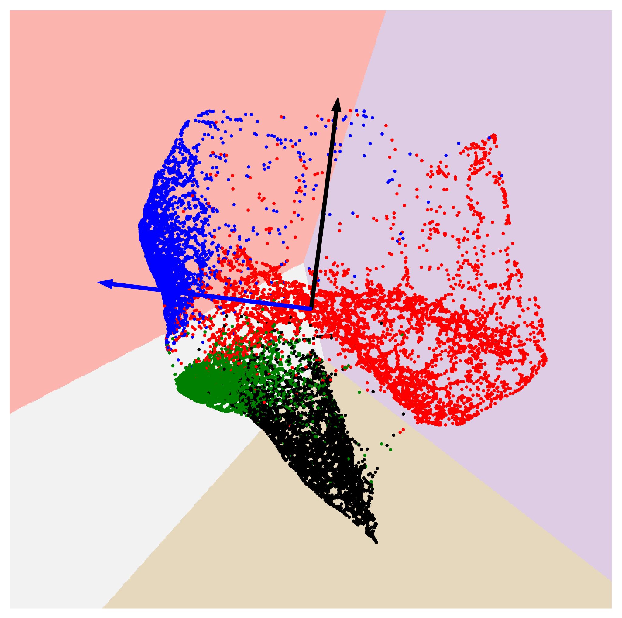
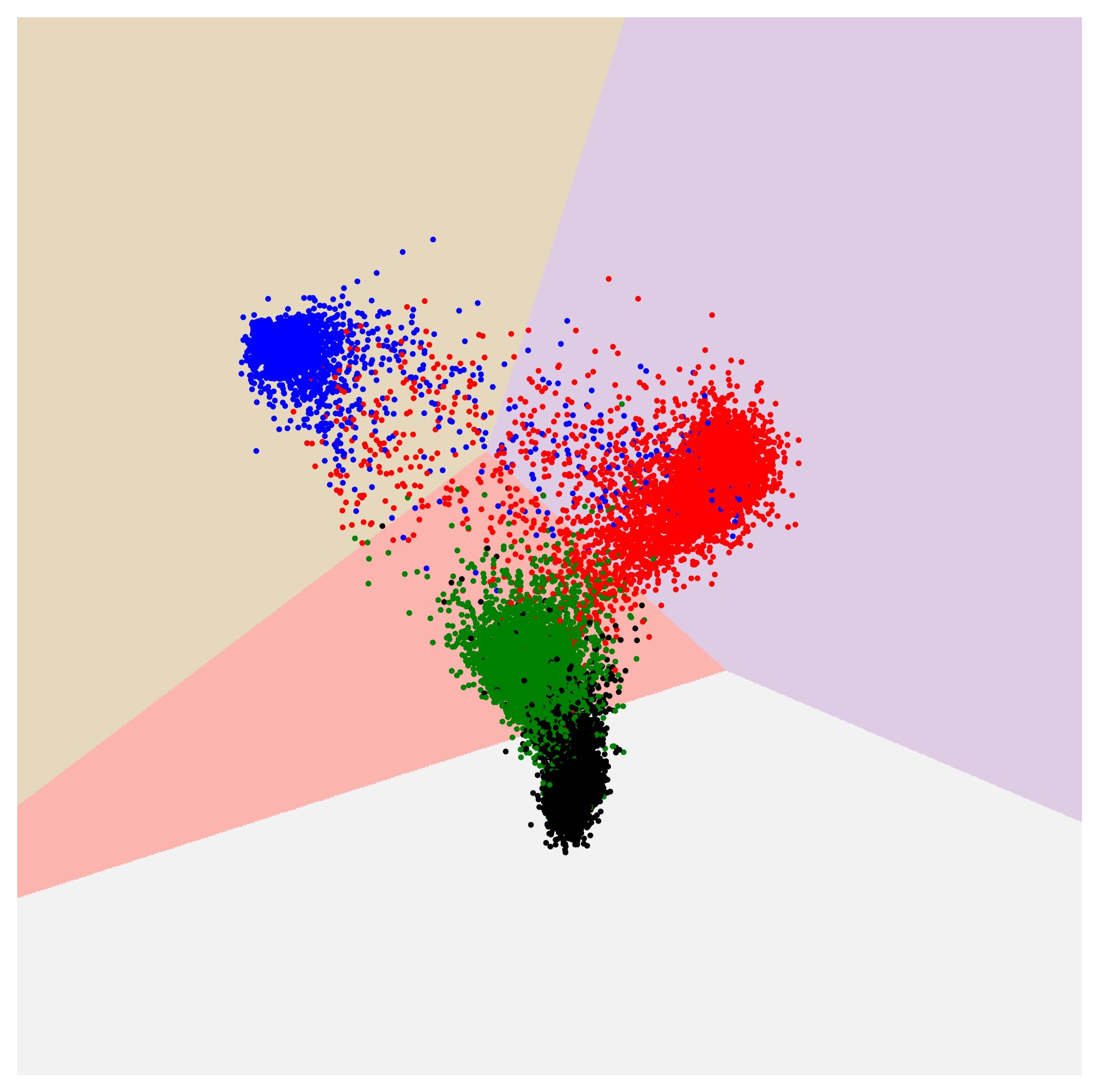
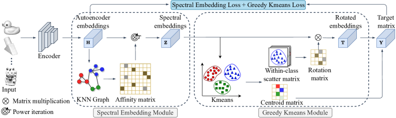
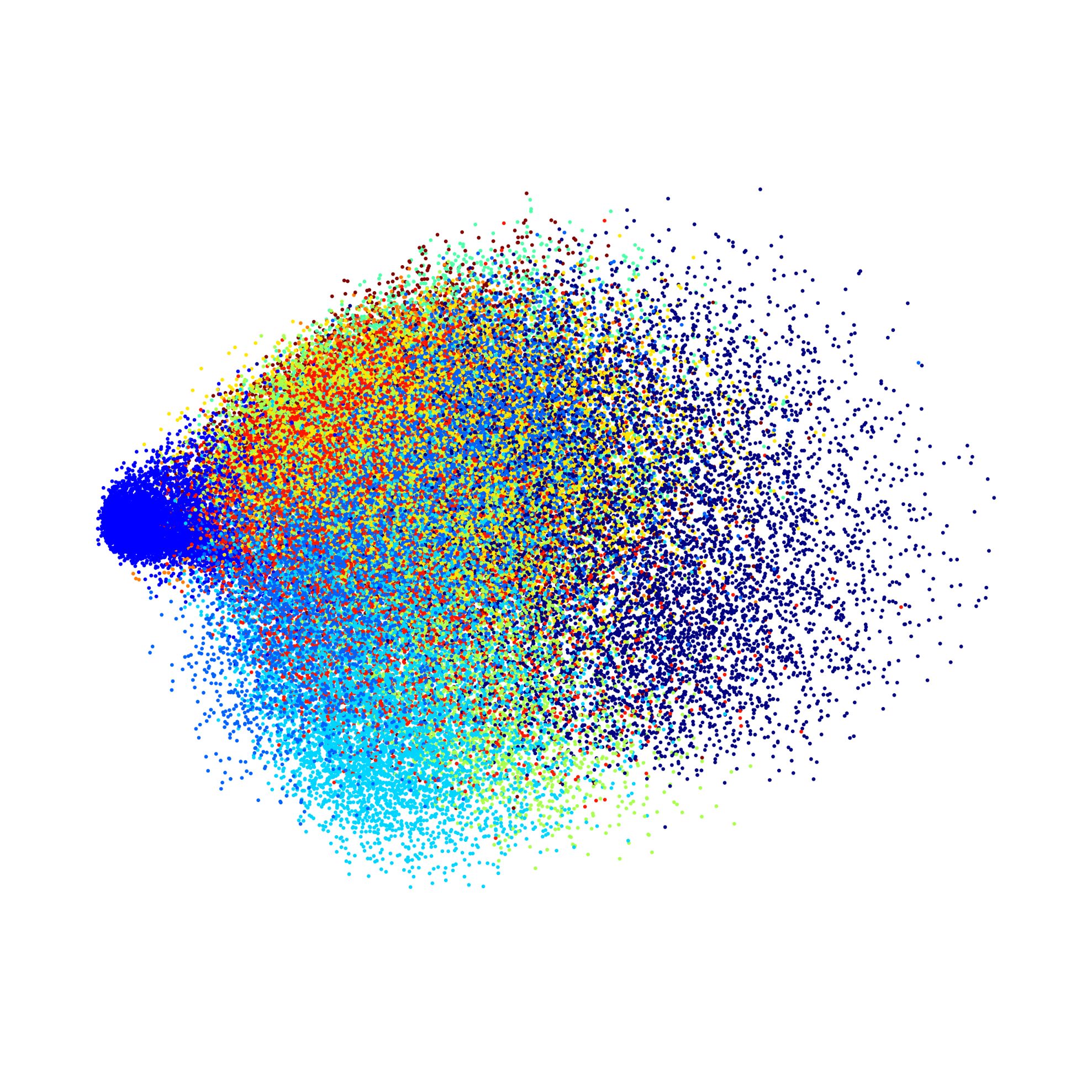
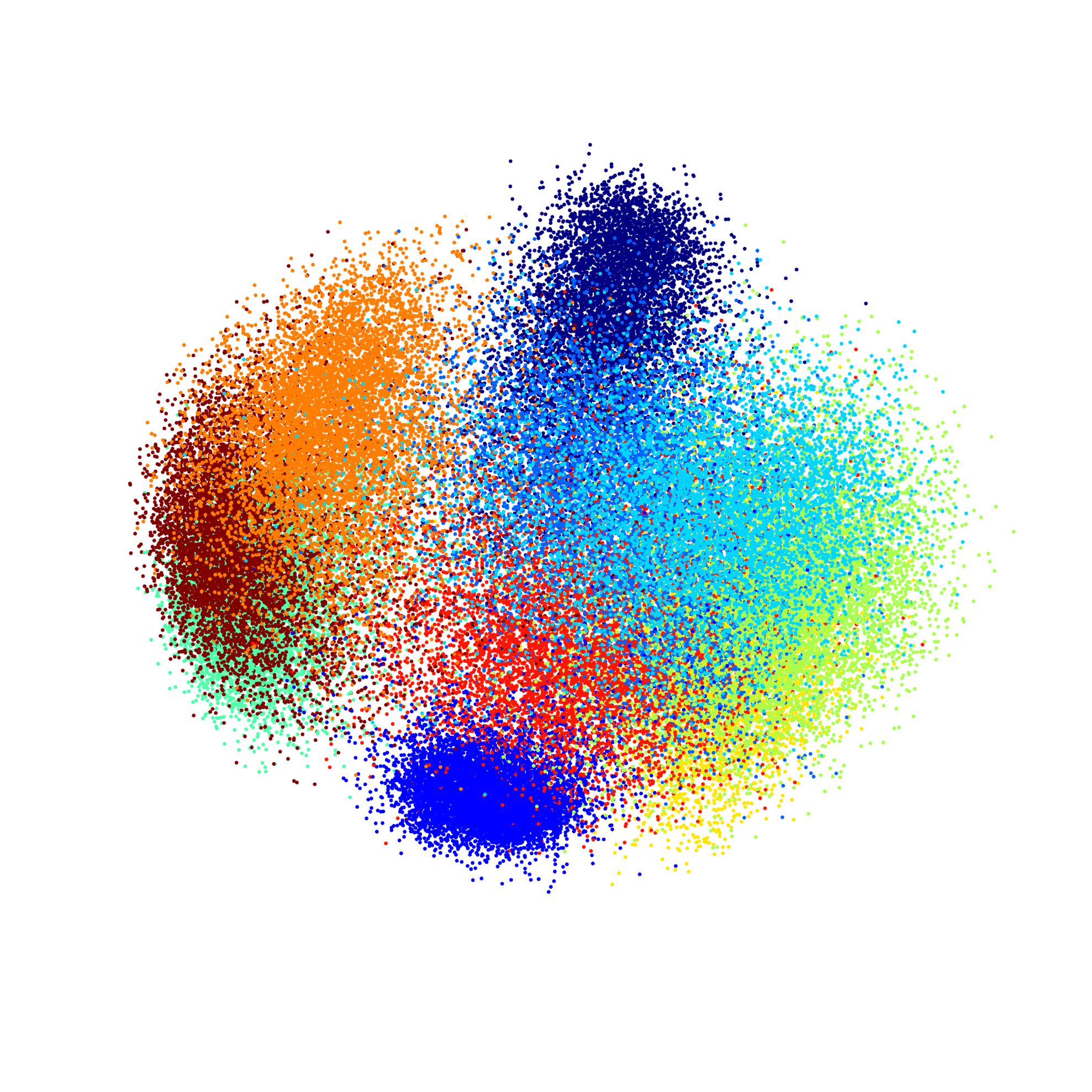
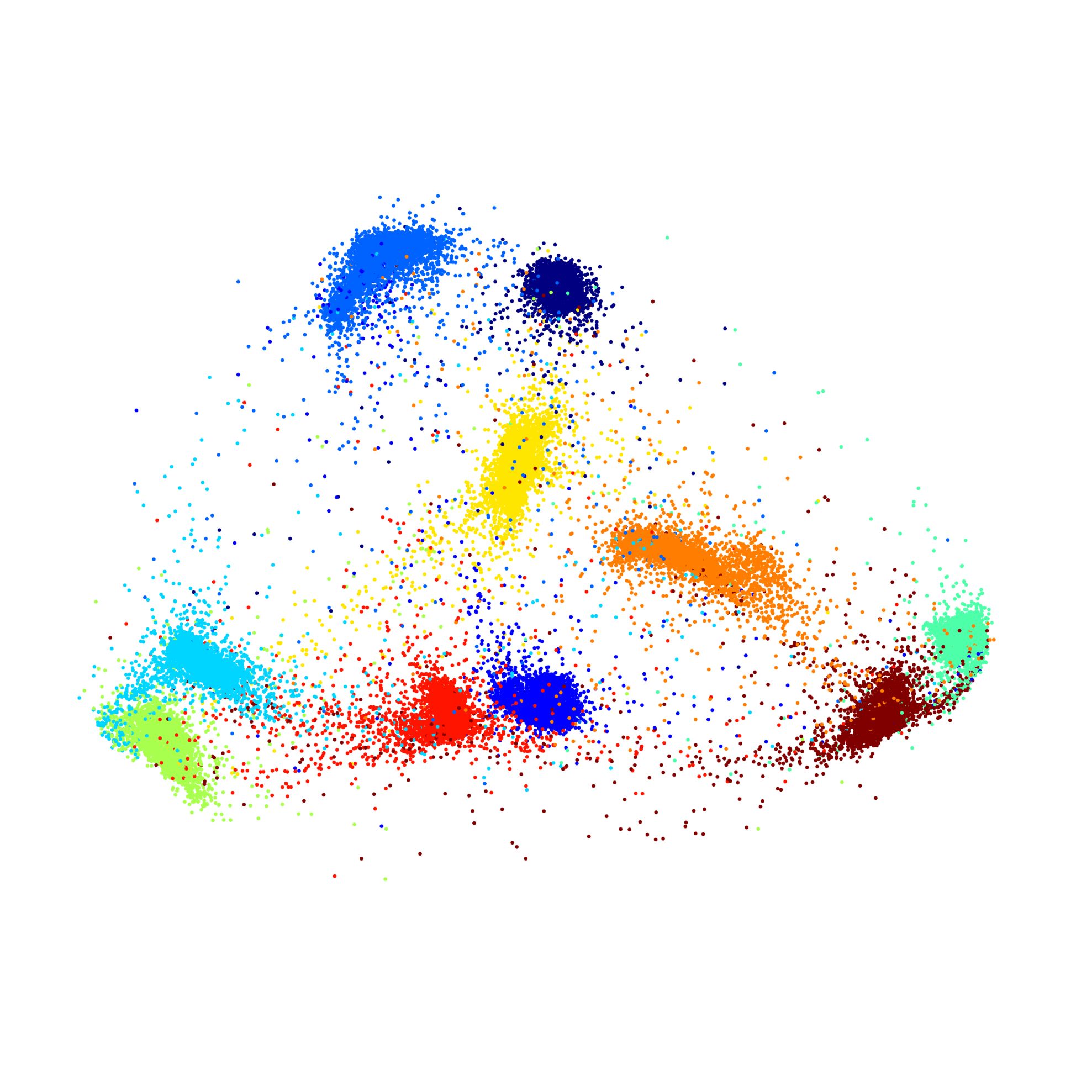
In this paper, we extend spectral clustering to a deep version called DSC to solve the two challenges mentioned above. DSC consists of two main modules: the spectral embedding module and the greedy Kmeans module. The former module efficiently embeds raw samples into a discriminative low-dimensional spectral embedding space using a deep autoencoder, which is similar to the spectral embedding step in spectral clustering but has a much lower time complexity. The high efficiency is attributed to replacing the labor-intensive eigendecomposition with the lightweight power iteration method. The latter greedy Kmeans module aims to make spectral embeddings Kmeans-friendly. The motivation is that while the spectral embeddings derived by graph Laplacian matrix are discriminative, they may not be optimally suited for Kmeans clustering, as the Kmeans objective is agnostic during their generation. For example, the spectral embeddings generated in Fig. 1(b) (viewing autoencoder (AE) embeddings in Fig. 1(a) as inputs) exhibit clear cluster structures, but they do not follow the isotropic Gaussian structures that Kmeans prefers. To address this issue, we propose fusing the Kmeans objective into the generation process of the spectral embeddings and propose a novel optimization strategy. Fig. 1(c) displays the spectral embedding after fusing Kmeans prior, showcasing cluster structures that are more aligned with Kmeans. To jointly optimize spectral embeddings and clustering, we seamlessly unify these two modules into a joint loss function and optimize this loss in an end-to-end manner.
Our main contributions can be summarized as:
-
•
We propose a deep spectral clustering method DSC that jointly optimizes spectral embeddings and Kmeans clustering by minimizing a novel joint loss.
-
•
To the best of our knowledge, this is the first work of deep joint spectral clustering.
-
•
Experiments on 7 real-world datasets demonstrate that DSC achieves state-of-the-art clustering performance.
II Related Work
In this section, we briefly review related works on spectral clustering, power-iteration-based clustering, deep spectral clustering, and deep clustering.
Spectral Clustering formulates the clustering task as a graph cut problem known as Min-Cut, drawing on the correlation between the eigenvalues of the graph Laplacian matrix and the connectivity of a graph. However, directly solving the Min-Cut problem yields degenerate clustering where a single outlier vertex forms a cluster. To promote balanced clusters, SC-Ncut [10] and SC-NJW [11] respectively introduce normalized cut, which have gained much popularity and promote further extensions.
Power-iteration-based clustering aims to reduce the computational cost of the eigendecomposition in spectral clustering. PIC [12] first proposes exploiting truncated power iteration to compute spectral embeddings. [13] provides a rigorous theoretical justification for power-iteration-based clustering methods. To reduce the redundancy of embeddings generated by power iteration, [14] introduces a procedure to orthogonalize these embeddings, and FUSE [15] utilizes Independent Component Analysis (ICA) [16] to make these embeddings pair-wise statistically independent. However, these methods still suffer from the high-dimensional data due to the shallow nature of their models. In contrast, we exploit the high representational power of deep neural networks to cope with the high-dimensional data.
Deep Spectral Clustering [8, 9, 17] combines spectral clustering with deep neural networks to improve spectral clustering. In the viewpoint of matrix reconstruction, Graphencoder [8] shows that both spectral clustering and autoencoder aim for the optimal low-rank reconstruction of the input affinity matrix. It thus proposes optimizing the reconstruction loss of the autoencoder instead of eigendecomposition. SpectralNet [9] learns to map raw samples into the eigenspace of the graph Laplacian matrix by deep neural networks. To prevent trivial solutions, it exploits QR decomposition [17] to ensure embedding orthogonality. Unlike these methods, we uniquely employ power iteration for spectral embedding learning.
Deep Clustering [18, 19, 20, 21, 22, 23, 24, 25, 26, 27, 28] has recently attracted significant attention. For example, DEC [18] pretrains an autoencoder with the reconstruction loss and performs Kmeans to obtain the soft cluster assignment of each sample. Then, it derives an auxiliary target distribution from the current soft cluster assignments, which emphasizes samples assigned with high confidence. Finally, it updates parameters by minimizing the Kullback–Leibler divergence between the soft cluster assignment and the auxiliary target distribution. The key idea behind DEC is to refine the clusters by learning from high-confidence assignments. JULE [19] introduces a recurrent framework for joint representation learning and clustering, where clustering is conducted in the forward pass and representation learning is conducted in the backward pass. DEPICT [20] consists of an autoencoder for learning the embedding space and a multinomial logistic regression layer functioning as a discriminative clustering model. DEPICT defines a clustering loss function using relative entropy minimization, regularized by a prior for the frequency of cluster assignments. As for deep subspace clustering, SENet [21] and EDESC [22] employ the neural network to learn a self-expressive representation. In very recent, some literature [23, 24] has explored Large Language Models (LLMs) [29] for clustering. Due to space limitations, we only review some classical methods here and interested readers can refer to [30] for a detailed review of deep clustering.
III Preliminaries
III-A Spectral Clustering
Let’s consider the problem of grouping samples into distinct clusters. The classical spectral clustering method SC-Ncut [10] converts the clustering task as a graph cut problem. Let denote the affinity matrix where element represents the similarity between samples and , denote the degree matrix where is the vector with all ones, denote the normalized affinity matrix, and denote the normalized graph Laplacian matrix where is the identity matrix. SC-Ncut optimizes the relaxed normalized cut objective:
| (1) |
where is the spectral embedding matrix (a relaxation of the discrete cluster assignment matrix), is the cost of graph cut, and the constraint item encourages -way partition. SC-Ncut performs eigendecomposition to solve that turns out to be the top minimum eigenvectors of (which are also the top maximum eigenvectors of ). Finally, SC-Ncut applies Kmeans to cluster the rows of and the resulting cluster assignments are assigned back to the original samples.
III-B Pretrained Autoencoder Embeddings
Autoencoder is a deep neural network that can unsupervisedly learn meaningful representations of data. It commonly consists of a trainable encoder that maps samples into a low-dimensional embedding space and a mirrored decoder that reconstructs the original samples from the embedding space . Autoencoder is trained by minimizing the reconstruction loss:
| (2) |
IV Deep Spectral Clustering
In this section, we elaborate on the proposed deep spectral clustering (DSC) method. As shown in Fig. 2, DSC has two main modules: the spectral embedding module and the greedy Kmeans module.
IV-A Spectral Embedding Module
Given data , we first pretrain a deep autoencoder to generate the -dimensional embeddings . We then compute the self-tuning affinity matrix [31]:
| (3) |
where is the autoencoder embedding of sample , is a scaling parameter that reflects local density information of , and denotes the -nearest neighbor of . We also compute the normalized affinity matrix .
Computing spectral embedding in Equation (1) via eigendecomposition is cost prohibitive when the number of samples is very large, due to its troublesome time complexity . Instead, we propose using power iteration to compute pseudo-eigenvectors, which has a much lower cost, requiring only a few matrix multiplications. Specifically, let , we repeatedly perform the below update rule:
| (4) |
The final output is termed spectral embeddings in this paper, which are linear combinations of the dominant eigenvectors of and contain rich cluster separation information. The multiplication can be regarded as independent matrix-vector multiplication , where the vector denotes the -th column of . Let and denote the eigenvalues and eigenvectors of respectively, we can rewrite the -th column of spectral embedding as:
| (5) | ||||
where represents the decomposition of using the basis and is the weight coefficient. As there exists an eigengap between the -th and -th eigenvalues (a basic assumption of spectral clustering [10]), will be a linear combination of the top maximum eigenvectors of after several iterations, and the ablation experiment in Table II indicate they are highly discriminative.
Choosing the iteration number is important for clustering, which trades off discrimination power with computational cost. An excessively large makes final spectral embeddings converge to the largest eigenvector of , which is a uniform vector and thus useless for clustering. To avoid this trivial solution, we introduce the acceleration metric to dynamically determine the appropriate , where . We set to be the smallest value of such that , where is a predefined threshold. For conciseness, the final spectral embeddings are hereafter denoted as .
Generalizing spectral embeddings to previously-unseen samples is non-trivial for traditional spectral clustering methods. To address this issue, we propose training the autoencoder to directly predict spectral embeddings, which can be formulated as a regression problem:
| (6) |
In this way, the encoder learns a deep mapping that embeds raw data into their spectral embedding space. Once trained, the deep mapping can be applied to out-of-sample data without needing to compute and eigendecompose their graph Laplacian matrix as shown by the experimental results in Table III.
IV-B Greedy Kmeans Module
After obtaining the spectral embeddings, traditional spectral clustering employs Kmeans to yield the final clustering results. This may result in underperformed clustering results, as the Kmeans objective is independent to the generation of these embeddings. We propose fusing the Kmeans objective into the generation process of the spectral embeddings, thereby obtaining Kmeans-friendly embeddings and potentially resulting in better clustering performance. Specifically, we employ Kmeans to find a partition of the spectral embeddings . The Kmeans objective is to minimize:
| (7) |
where denotes the set of samples assigned to the -th cluster, denotes the centroid of .
To generate Kmeans-friendly embeddings, a direct idea is to minimize Objective (7) by pulling samples closer to their respective cluster centroids. To this end, we propose a greedy optimization strategy: pulling samples towards their cluster centroids only in the direction that exhibits the worst cluster structures. This greedy strategy is easier to optimize than naively pulling samples in all directions. To find the direction of the worst cluster structure in the spectral embedding space , we rotate using an orthogonal matrix (). We select the linear rotation transformation for two reasons: (1) the linearity is sufficient for this task, as the deep autoencoder has already learned the non-linear relationships. (2) the orthogonal matrix maintains the Euclidean distances between embeddings and thus preserves all cluster structures in . We use the Kmeans objective as a prior—the smaller the Kmeans objective value, the better the cluster structures—to help solve for . The Kmeans objective value along the direction of is:
| (8) |
where is the within-class scatter matrix of Kmeans. The Kmeans Objective (7) w.r.t thus can be rewritten as:
| (9) |
The solution of contains the eigenvectors of , and the eigenvalues (the Kmeans objective value) indicate the quality of cluster structures in the corresponding eigenvectors. The smaller the eigenvalue, the better the cluster structures along its eigenvector direction. The solution can always be found as is symmetric and thus orthogonally diagonalizable, and the computational cost is negligible as the size of is much smaller than the raw data, i.e., . We sort these eigenvectors in in ascending order w.r.t. their eigenvalues. Thus, the direction of the last eigenvector whose eigenvalue is the largest, has the worst quality of the cluster structure. Fig. 1(b) displays an example, where the black arrow denotes .
After obtaining the largest eigenvector , we will pull samples towards their cluster centroids in the direction of . Specifically, we construct a target matrix and then replace the last column of with a pulling target vector . The -th element of is defined as , i.e., the projection of ’s cluster mean into the direction of the largest eigenvector. The objective is to minimize the difference between spectral embeddings and the target matrix in the direction of :
| (10) |
where is the last column of the identity matrix . In this paper, we solve for and minimize the Kmeans objective along in an alternate manner, thus terming the above equation as greedy Kmeans loss.
| Dataset | USPS | FASHION | FASHION-test | MNIST | MNIST-test | COIL20 | FRGC | |||||||
|---|---|---|---|---|---|---|---|---|---|---|---|---|---|---|
| Method | ACC | NMI | ACC | NMI | ACC | NMI | ACC | NMI | ACC | NMI | ACC | NMI | ACC | NMI |
| Kmeans | 66.81 | 62.62 | 47.57 | 51.22 | 52.25 | 58.78 | 53.22 | 49.96 | 54.24 | 50.00 | 25.28 | 67.17 | 12.63 | 18.27 |
| SC-Ncut | 62.51 | 69.48 | 52.06 | 59.05 | 52.24 | 58.76 | 63.15 | 73.25 | 59.54 | 69.12 | 60.35 | 72.42 | 27.50 | 33.03 |
| SC-NJW | 66.91 | 61.66 | 55.17 | 62.82 | 46.15 | 50.31 | 55.17 | 62.82 | 56.13 | 48.62 | 70.14 | 79.42 | 42.45 | 51.52 |
| PIC | 61.79 | 58.67 | 44.18 | 54.21 | 46.74 | 50.59 | 49.89 | 60.67 | 51.23 | 54.05 | 18.61 | 38.52 | 16.04 | 11.44 |
| FUSE | 57.55 | 56.86 | 52.10 | 53.44 | 49.00 | 52.00 | 63.89 | 69.64 | 77.00 | 72.00 | 23.47 | 37.17 | 17.43 | 12.25 |
| SE-ISR | 60.55 | 65.60 | 57.38 | 57.22 | 51.44 | 55.15 | 57.56 | 55.06 | 67.36 | 64.25 | 69.51 | 82.79 | 36.23 | 44.28 |
| DEC | 69.75 | 68.66 | 51.80 | 55.23 | 59.20 | 59.52 | 81.27 | 75.70 | 75.86 | 69.89 | 53.47 | 70.81 | 32.13 | 40.64 |
| DEKM | 78.87 | 80.51 | 58.89 | 62.55 | 52.36 | 60.27 | 95.75 | 91.06 | 83.99 | 80.86 | 72.62 | 81.97 | 37.29 | 49.32 |
| Graphencoder | 20.66 | 12.65 | - | - | 34.28 | 31.19 | 14.84 | - | - | 5.55 | 45.49 | 59.87 | 12.84 | 7.42 |
| SpectralNet | 78.12 | 81.36 | 53.07 | 59.07 | 52.58 | 58.36 | 60.95 | 67.02 | 61.91 | 68.21 | 64.03 | 86.39 | 31.52 | 43.60 |
| DEPICT | 96.40 | 92.70 | 50.38 | 57.04 | 50.74 | 51.74 | 96.50 | 91.70 | 96.50 | 91.50 | 74.38 | 81.97 | 47.00 | 61.00 |
| SENet | 80.60 | 75.37 | 66.19 | 66.08 | 60.24 | 64.14 | 96.80 | 91.69 | 96.27 | 91.94 | 44.58 | 71.06 | 46.72 | 27.71 |
| EDESC | 72.90 | 69.20 | 55.13 | 58.41 | 56.91 | 56.79 | 74.15 | 66.74 | 66.23 | 56.41 | 70.42 | 78.16 | 28.76 | 30.53 |
| WEC-MMD | - | - | 62.20 | 62.96 | - | - | 96.74 | 92.23 | - | - | 82.71 | 87.80 | - | - |
| DML-DSL | 84.41 | 79.47 | 63.20 | 64.80 | 55.34 | 57.50 | 96.33 | 91.22 | 95.16 | 89.23 | 88.38 | 70.54 | 79.12 | 46.75 |
| DSC | 97.26 | 93.00 | 64.62 | 67.98 | 62.56 | 68.81 | 97.80 | 94.10 | 96.86 | 92.36 | 81.88 | 89.53 | 41.55 | 58.27 |
IV-C Joint Loss Function
We consider jointly optimizing the spectral embedding loss and greedy Kmeans loss in an end-to-end way. To this end, we slightly modify the spectral embedding Loss (6). Instead of forcing the encoder to predict the whole spectral embeddings , we encourage the encoder to predict in all directions except for the direction that contains the worst cluster structures:
| (11) |
where we use the fact the first columns of and are the same, and is the first columns of the identity matrix . This above loss can still learn meaningful embeddings, as most discriminative information exists in the directions with good cluster structures. Finally, we combine the above loss with the greedy Kmeans Loss (10) seamlessly:
| (12) |
Algorithm 1 shows the pseudo-code of DSC. The time complexity of DSC for training is and for inference is , where denotes the number of neurons in the autoencoder. Since , , and are constants, the time complexity for training is bounded by and for inference is bounded by . In addition, the space complexity is .
| Dataset | USPS | FASHION | FASHION-test | MNIST | MNIST-test | COIL20 | FRGC | |||||||
|---|---|---|---|---|---|---|---|---|---|---|---|---|---|---|
| Method | ACC | NMI | ACC | NMI | ACC | NMI | ACC | NMI | ACC | NMI | ACC | NMI | ACC | NMI |
| AE+Kmeans | 83.93 | 80.05 | 56.36 | 61.87 | 60.40 | 62.30 | 94.43 | 87.51 | 91.07 | 81.87 | 68.72 | 80.34 | 37.04 | 46.15 |
| AE+SC-Ncut | 76.44 | 74.86 | 56.33 | 59.38 | 54.76 | 59.56 | 93.59 | 86.29 | 83.75 | 76.61 | 69.91 | 80.51 | 41.52 | 52.29 |
| AE+SE | 96.21 | 91.29 | 64.23 | 67.63 | 62.50 | 68.65 | 97.34 | 93.28 | 96.01 | 90.92 | 77.02 | 86.97 | 40.68 | 56.84 |
| AE+GK | 86.67 | 82.15 | 56.91 | 62.25 | 61.49 | 62.84 | 95.68 | 89.68 | 93.37 | 85.54 | 71.56 | 80.85 | 41.17 | 54.06 |
| AE+SE+GK (DSC) | 97.26 | 93.00 | 64.62 | 67.98 | 62.56 | 68.81 | 97.80 | 94.10 | 96.86 | 92.36 | 81.88 | 89.53 | 41.55 | 58.27 |
V Experimental Evaluation
In this section, we first compare DSC with 15 clustering methods on 7 benchmark datasets. We then conduct ablation study to evaluate the effect of each module of DSC. Subsequently, we evaluate the generalization ability by conducting out-of-sample experiment. After that, we evaluate the efficiency of each method by comparing their running time. Finally, we visualize the learned embeddings at different training stages.
Datasets and Metrics. We utilize 7 benchmark datasets that cover handwritten digits, fashion products, multi-view objects, and human faces: USPS [32], MNIST[33], FASHION [2], COIL-20 [34], FRGC [19]. The first three datasets each contains 10 clusters, while the latter two datasets each contains 20 clusters. Unless explicitly specified, we concatenate the training and test sets of each dataset for evaluation. We use two standard metrics to evaluate clustering performance: Clustering Accuracy (ACC) and Normalized Mutual Information (NMI). Both metrics range from 0 to 1, and higher values indicate better clustering performance.
Implementation Details. We employ a convolutional autoencoder for evalution. The encoder consists of three stacked convolutional layers with 32, 64, and 128 channels respectively and a linear embedding layer with 10 neurons. The decoder is a mirrored version of the encoder layers. The parameter for constructing the self-tuning affinity matrix is set to 7. The early stopping threshold of power iteration is set to 0.01, and the maximum update iteration number is limited to 15. The batch size is set to 256 for pretraining the autoencoder and 32 for clustering training. In each iteration of clustering training, we use 40 mini-batches of samples. The autoencoder is trained by the Adam optimizer with parameters , , . We pretrain the autoencoder with 200 epochs and stop the clustering training when less than 0.5% of samples change their cluster assignments between two consecutive iterations. We fix these parameter settings for all the datasets. Our code is available at https://github.com/spdj2271/DSC.
V-A Comparisons to State-of-the-Art Methods
We compare the proposed DSC with 6 conventional clustering methods and 9 deep clustering methods. The conventional clustering methods contain: Kmeans [1]; two common spectral clustering methods: spectral clustering with normalized cuts (SC-Ncut) [10] and NJW spectral clustering (SC-NJW) [11]; three improved spectral clustering methods: power iteration clustering (PIC) [12], full spectral clustering (FUSE) [15], spectral clustering with simultaneous spectral embedding and spectral rotation (SE-ISR) [35]. The deep clustering methods contain: deep embedded clustering (DEC) [18], deep embedded Kmeans clustering (DEKM) [36], autoencoder-based spectral graph clustering (Graphencoder) [8], spectral clustering network (SpectralNet) [9], deep embedded regularized clustering (DEPICT) [20], self-expressive clustering network (SENet) [21], deep embedded subspace clustering (EDESC) [22], deep multi-representation clustering (DML-DS) [37], and deep Wasserstein embedding clustering (WEC-MMD) [38].
Table I shows the overall clustering results on the 7 benchmark datasets. DSC achieves much better clustering performance than all the shallow clustering methods (the first 6 rows in Table I). Similar to DSC, SC-ISR optimizes spectral embedding and spectral rotation simultaneously, but DSC significantly outperforms it. This large margin in performance is due to the powerful representation capability of the neural networks. Compared with deep clustering methods, DSC achieves better results on most datasets, which can be attributed to the effective simultaneous representation (spectral embedding) learning and clustering strategy.
V-B Ablation Study
DSC consists of two main modules: the spectral embedding (SE) module and the greedy Kmeans (GK) module. To evaluate each module’s effectiveness, we first detect clusters on the pretrained autoencoder embeddings with Kmeans (AE+Kmeans) and SC-Ncut (AE+SC-Ncut), whose clustering results serve as the baselines. We then train a model (AE+SE) by only minimizing and report clustering results by conducting posthoc Kmeans clustering on the learned spectral embeddings. Subsequently, we train another model (AE+EM) by only minimizing , where Kmeans is applied on the autoencoder embeddings to obtain the rotation matrix and generate the target matrix. Table II indicates that both the SE and GK modules improve the clustering performance. The SE module plays a key role, which helps to reduce the dimensionality of the data while capturing the essential cluster structural information. The GK module could improve the performance to some extent, which aligns with its purpose of fine-tuning the spectral embeddings to be Kmeans-friendly.
| Dataset | MNIST-testMNIST-train | FASHION-testFASHION-train | ||
|---|---|---|---|---|
| Method | ACC | NMI | ACC | NMI |
| SpectralNet | 61.9161.31 | 68.2166.35 | 52.5852.74 | 58.3658.88 |
| DSC | 96.8696.06 | 92.3690.59 | 62.5662.62 | 69.3068.78 |
V-C Evaluation of Generalization Ability
We compare the generalization ability of our DSC with the existing deep spectral clustering method SpectralNet by applying the trained models to the previously-unseen samples. We respectively train DSC and SpectralNet on FASHION-test and MNIST-test datasets and then evaluate these two models on the FASHION-train and MNIST-train datasets. For a more challenging evaluation setting, we select to conduct the generalization experiments on the larger train datasets (60,000 samples) rather than the test datasets (10,000 samples). Table III shows that DSC exhibits better generalization performance compared to SpectralNet.
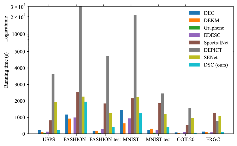
V-D Running Time Comparison
We compare the running time (including the pretraining time of autoencoders) of each deep clustering model on all the datasets and the results are presented in Figure 3. The experiment is conducted on a server equipped with one Nvidia GeForce GTX 1050Ti GPU. Our DSC outperforms SpectralNet, DEPICT, and SENet with an obvious advantage. Specifically, the running time of DEPICT dramatically grows on large datasets (FASHION and MNIST), leading to manual stopping after 30,000 seconds on the FASHION dataset. In contrast, DSC only takes 1,900 seconds to complete the FASHION dataset. Despite the efficiency advantages exhibited by other competitors, such as DEC, DEKM, Graphenc, and EDESC, their clustering performance is clearly unsatisfactory as demonstrated in Table I. Our DSC requires a similar running time to these models but achieves significantly higher clustering performance. In fact, the majority running time of DSC expends on the pretraining of autoencoder, which is requisite for any autoencoder-based clustering methods.
V-E Embedding Space Comparison
We visualize the embedding space at different training stages of DSC on the MNIST dataset in Fig. 4. We conduct Principal Component Analysis (PCA) [4] on the embeddings and then select the first three principal components for visualization. Fig. 4(a) shows that raw samples are in a chaotic status and there are no obvious cluster structures. Compared with the pretrained autoencoder embeddings in Fig. 4(b), the embeddings learned by DSC in Fig. 4(c) are well-separated, exhibiting much better cluster structures.
VI Conclusion
In this paper, we have proposed a novel deep spectral clustering method called DSC. It combines the deep autoencoder and power iteration to efficiently learn the discriminative spectral embeddings. DSC also introduces a greedy Kmeans objective to make the spectral embeddings Kmeans-friendly. Experiments on seven real-world datasets indicate that DSC achieves state-of-the-art clustering performance. In the future, we will extend DSC to cluster multi-view data.
VII Acknowledgments
We thank the anonymous reviewers for their valuable and constructive comments. This work was supported partially by the National Natural Science Foundation of China (grant #62176184), the National Key Research and Development Program of China (grant #2020AAA0108100), and the Fundamental Research Funds for the Central Universities of China.
References
- [1] S. Lloyd, “Least squares quantization in pcm,” IEEE Trans. Inf. Theory, 1982.
- [2] H. Xiao, K. Rasul, and R. Vollgraf, “Fashion-mnist: a novel image dataset for benchmarking machine learning algorithms,” 2017.
- [3] S. Wang, F. Chen, and J. Fang, “Spectral clustering of high-dimensional data via nonnegative matrix factorization,” in IJCNN, 2015.
- [4] K. Pearson, “Liii. on lines and planes of closest fit to systems of points in space,” The London, Edinburgh, and Dublin Philosophical Magazine and Journal of Science, 1901.
- [5] D. D. Lee and H. S. Seung, “Learning the parts of objects by non-negative matrix factorization,” Nature, 1999.
- [6] Y. Yang, F. Shen, Z. Huang, and H. T. Shen, “A unified framework for discrete spectral clustering.,” in IJCAI, 2016.
- [7] Y. Pang, J. Xie, F. Nie, and X. Li, “Spectral clustering by joint spectral embedding and spectral rotation,” TCYB, 2018.
- [8] F. Tian, B. Gao, Q. Cui, E. Chen, and T.-Y. Liu, “Learning deep representations for graph clustering,” in AAAI, 2014.
- [9] U. Shaham, K. Stanton, H. Li, R. Basri, B. Nadler, and Y. Kluger, “Spectralnet: Spectral clustering using deep neural networks,” in ICLR, 2018.
- [10] J. Shi and J. Malik, “Normalized cuts and image segmentation,” TPAMI, 2000.
- [11] A. Y. Ng, M. I. Jordan, Y. Weiss, et al., “On spectral clustering: Analysis and an algorithm,” NeurIPS, 2002.
- [12] F. Lin and W. W. Cohen, “Power iteration clustering,” in ICML, 2010.
- [13] C. Boutsidis, P. Kambadur, and A. Gittens, “Spectral clustering via the power method-provably,” in ICML, 2015.
- [14] H. Huang, S. Yoo, D. Yu, and H. Qin, “Diverse power iteration embeddings: Theory and practice,” TKDE, 2015.
- [15] W. Ye, S. Goebl, C. Plant, and C. Böhm, “Fuse: Full spectral clustering,” in SIGKDD, 2016.
- [16] E. G. Learned-Miller and J. W. F. Iii, “Ica using spacings estimates of entropy,” J. Mach. Learn. Res., 2003.
- [17] A. S. Householder, “Unitary triangularization of a nonsymmetric matrix,” Journal of the ACM (JACM).
- [18] J. Xie, R. Girshick, and A. Farhadi, “Unsupervised deep embedding for clustering analysis,” in ICML, 2016.
- [19] J. Yang, D. Parikh, and D. Batra, “Joint unsupervised learning of deep representations and image clusters,” in CVPR, 2016.
- [20] K. Ghasedi Dizaji, A. Herandi, C. Deng, W. Cai, and H. Huang, “Deep clustering via joint convolutional autoencoder embedding and relative entropy minimization,” in ICCV, 2017.
- [21] S. Zhang, C. You, R. Vidal, and C.-G. Li, “Learning a self-expressive network for subspace clustering,” in CVPR, 2021.
- [22] J. Cai, J. Fan, W. Guo, S. Wang, Y. Zhang, and Z. Zhang, “Efficient deep embedded subspace clustering,” in CVPR, 2022.
- [23] S. Kwon, J. Park, M. Kim, J. Cho, E. K. Ryu, and K. Lee, “Image clustering conditioned on text criteria,” in ICLR, 2024.
- [24] Y. Zhang, Z. Wang, and J. Shang, “Clusterllm: Large language models as a guide for text clustering,” in EMNLP, 2023.
- [25] L. Miklautz, M. Teuffenbach, P. Weber, R. Perjuci, W. Durani, C. Böhm, and C. Plant, “Deep clustering with consensus representations,” in ICDM, 2022.
- [26] C. Leiber, L. G. Bauer, M. Neumayr, C. Plant, and C. Böhm, “The dipencoder: Enforcing multimodality in autoencoders,” in SIGKDD, 2022.
- [27] C. Leiber, L. G. Bauer, B. Schelling, C. Böhm, and C. Plant, “Dip-based deep embedded clustering with k-estimation,” in SIGKDD, 2021.
- [28] L. Miklautz, L. G. Bauer, D. Mautz, S. Tschiatschek, C. Böhm, and C. Plant, “Details (don’t) matter: Isolating cluster information in deep embedded spaces.,” in IJCAI, 2021.
- [29] J. Achiam, S. Adler, S. Agarwal, L. Ahmad, I. Akkaya, F. L. Aleman, D. Almeida, J. Altenschmidt, S. Altman, S. Anadkat, et al., “Gpt-4 technical report,” 2023.
- [30] S. Zhou, H. Xu, Z. Zheng, J. Chen, J. Bu, J. Wu, X. Wang, W. Zhu, M. Ester, et al., “A comprehensive survey on deep clustering: Taxonomy, challenges, and future directions,” 2022.
- [31] L. Zelnik-Manor and P. Perona, “Self-tuning spectral clustering,” NeurIPS, 2004.
- [32] J. J. Hull, “A database for handwritten text recognition research,” TPAMI, 1994.
- [33] Y. LeCun, L. Bottou, Y. Bengio, and P. Haffner, “Gradient-based learning applied to document recognition,” 1998.
- [34] S. A. Nene, S. K. Nayar, H. Murase, et al., “Columbia object image library (coil-100),” 1996.
- [35] Z. Wang, X. Dai, P. Zhu, R. Wang, X. Li, and F. Nie, “Fast optimization of spectral embedding and improved spectral rotation,” TKDE, 2021.
- [36] W. Guo, K. Lin, and W. Ye, “Deep embedded k-means clustering,” in ICDMW, 2021.
- [37] M. Sadeghi and N. Armanfard, “Deep multirepresentation learning for data clustering,” TNNLS, 2023.
- [38] J. Cai, Y. Zhang, S. Wang, J. Fan, and W. Guo, “Wasserstein embedding learning for deep clustering: A generative approach,” TMM, 2024.