Classification Drives Geographic Bias in Street Scene Segmentation

Abstract

Previous studies showed that image datasets lacking geographic diversity can lead to biased performance in models trained on them. While earlier work studied general-purpose image datasets (e.g., ImageNet) and simple tasks like image recognition, we investigated geo-biases in real-world driving datasets on a more complex task: instance segmentation. We examined if instance segmentation models trained on European driving scenes (Eurocentric models) are geo-biased. Consistent with previous work, we found that Eurocentric models were geo-biased. Interestingly, we found that geo-biases came from classification errors rather than localization errors, with classification errors alone contributing $10$-$90\%$ of the geo-biases in segmentation and $19$-$88\%$ of the geo-biases in detection. This showed that while classification is geo-biased, localization (including detection and segmentation) is geographically robust. Our findings show that in region-specific models (e.g., Eurocentric models), geo-biases from classification errors can be significantly mitigated by using coarser classes (e.g., grouping car, bus, and truck as $4$-wheeler).

1 Introduction

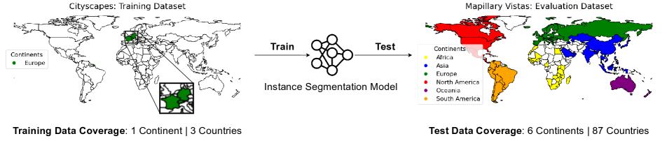
Figure 1: Evaluating Eurocentric models on the Mapillary Vistas dataset

Image datasets like ImageNet [6] and OpenImages [10] have been crucial in advancing computer vision research. However, they have a notable drawback — they lack geographic diversity. These datasets primarily contain images from Western countries (Europe and the USA), which do not reflect the diversity of visual scenes worldwide. Previous studies have shown that models trained on biased datasets perform well when tested on images from regions (countries or continents) well-represented in the dataset. However, these models perform poorly on images from regions underrepresented in the dataset [15, 5]. This variation in model performance across regions, stemming from a lack of geographic diversity in the training dataset, is often referred to as geographic bias (or geo-bias for short).

Identifying and mitigating geo-bias is crucial to avoid the need for retraining models when they encounter images from new geographic locations. Previous studies on geo-biases in computer vision have been useful but face several limitations [15, 5]. First, they studied general-purpose datasets like ImageNet and OpenImages. These datasets have simple scenes with $1$-$2$ objects of interest per image. Hence, they rarely represent real-world scenarios. Second, previous work examined geo-biases for image recognition, a coarse-grained task. No prior work has examined geo-biases in tasks involving both classification and localization (e.g., detection or segmentation).

While general-purpose image datasets are popular, they are not the only type of image datasets used in vision research. Some image datasets are also designed for real-world applications — like driving datasets for autonomous driving. Driving datasets contain images that represent complex real-world street scenes captured from a dashcam. Like general-purpose datasets, well-known driving datasets (e.g., BDD100K [17], Cityscapes [4], nuScenes [2]) are primarily collected in Western countries. Previous work on geo-biases would suggest that vision models trained on Western-centric driving datasets will perform poorly on scenes from regions not represented in the training dataset. However, no study has investigated if models trained on Western-centric driving datasets also exhibit geo-biases.

Our study is the first to answer the following questions: Do vision models trained on Eurocentric driving datasets perform poorly on continents outside Europe? If there are performance variations among continents (i.e., geo-biases), what is the root cause? We focused on instance segmentation models pre-trained on Cityscapes, a dataset of urban street scenes widely used in computer vision research. All images in Cityscapes are from cities in Germany or neighboring countries. We refer to models pre-trained on Cityscapes as Eurocentric models. We evaluated these Eurocentric models on out-of-distribution images from the Mapillary Vistas dataset (Vistas) [12], a driving dataset containing images from six continents (refer to Figure 1).

We examined geo-biases in instance segmentation models, measuring performance disparities in detection (bounding boxes) and segmentation. We found that Eurocentric models were geo-biased for several classes (rider, bicycle, bus, truck, motorcycle). Interestingly, we found that geo-biases were not caused by localization errors but rather by classification errors. We introduce a new class-merging strategy to isolate the contribution of classification errors on geo-bias. In class-merging, we combine classes that are often misclassified with each other: person-rider (people), car-bus-truck (vehicles with $\geq 4$ wheels), and motorcycle-bicycle ($2$-wheelers). For the geo-biased classes, we found that classification errors alone accounted for $19$-$88\%$ of the geo-biases in detection and $10$-$90\%$ of the geo-biases in segmentation. This shows that classification is highly geo-biased, but localization is more geographically robust.

Our findings show that if a user aims to apply region-specific models (like Eurocentric models) globally, it is preferable to use coarser class labels (e.g., $4$-wheeler) rather than fine-grained ones (e.g., car, bus, truck). This significantly reduces the geo-biases from classification errors. Geo-biases in localization are minimal, but further research is needed to mitigate these biases.

In summary, our contributions are as follows: (1) We are the first to examine geo-biases in driving datasets on a localization task like instance segmentation; (2) We conduct a systematic analysis of instance segmentation models to identify the root cause of geo-biases; and (3) We propose a new class-merging strategy to measure the isolated contribution of classification errors to geo-bias.

2 Related Work

Previous work examined geo-biases in general-purpose datasets like ImageNet, OpenImages, and DollarStreet. Shankar et al. [15] showed that models trained using datasets biased towards Western countries (ImageNet [6] and OpenImages [10]) had poor performance for countries underrepresented in the training dataset (e.g., Ethiopia and Pakistan) for fine-grained classes (e.g., groom, police officer, vendor). Through experiments with the ImageNet and DollarStreet [14] datasets, De Vries et al. [5] showed that models trained using ImageNet, which is dominated by images from high-income countries, had poorer performance on images from low-income countries for fine-grained classes in DollarStreet (e.g., spices, soap). Rojas et al. [14] showed that training models on DollarStreet, which was more diverse in terms of geography and income than ImageNet, resulted in more balanced performance across geographies and income levels. Gustafson et al. [7] conducted an in-depth analysis of DollarStreet to understand why geo-biases occurred across geographies and income levels. They annotated DollarStreet images with factor labels (e.g., texture, shape, lighting, occlusion) and showed that factors like texture and occlusion contributed to the poor performance of models in low-income continents (e.g., Africa and Asia) in DollarStreet.

Kalluri et al. [9] proposed GeoNet, a general-purpose dataset to study geographic adaptation between the USA and India. They showed that unsupervised domain adaption (UDA) models performed equal to or worse than baseline models trained only using source domain data. This indicated that the domain shift between the USA and India is large, and better UDA models are needed to bridge the domain gap. Ramaswamy et al. [13] proposed GeoDE, a geographically diverse general-purpose dataset created by soliciting images from people across six continents. They showed that models trained on a combined set of ImageNet and GeoDE images performed better on DollarStreet across geographies than models trained solely on ImageNet.

Prior works on geo-biases either examined existing general-purpose datasets or proposed new (more diverse) general-purpose datasets. Most of this work has examined geo-bias in simple tasks like image classification. Geo-bias in complex tasks like localization (e.g., detection, segmentation) is largely unexplored. In our work, we studied geo-bias in driving datasets as they represent real-world scenarios like street scenes. We are the first to investigate geo-biases in instance segmentation models.

3 Experiment Design

3.1 Instance segmentation task

We evaluated driving datasets on the instance segmentation task. We chose instance segmentation for several reasons. Instance segmentation is important for scene understanding in autonomous driving use cases. Unlike image recognition labels (studied in previous work) and bounding box annotations, instance segmentation offers pixel-level localization, which could be important when examining geo-biases. While semantic segmentation also offers pixel-level localization, it labels objects at the class level. As a result, the global-intersection-over-union (global-IoU) metric gives more weight to the larger objects (objects occupying more area) in a class. This size bias in semantic segmentation could mask other important factors causing geo-bias.

((a))

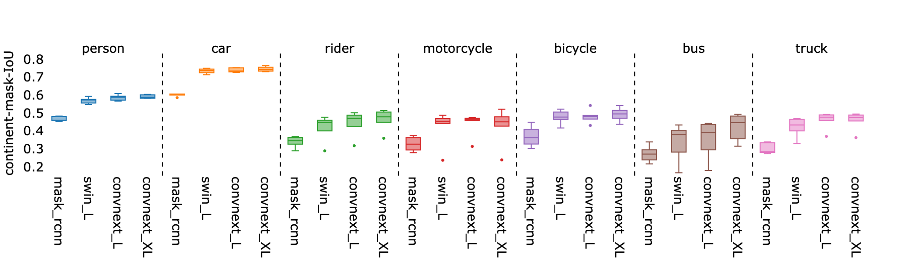
((b))

Figure 2: Detection and segmentation box plots. Each box plot is made with $6$ data points. Here, a data point refers to the average performance (IoU) of a model for a class in a continent. In both figures, while person and car hold minimal geo-biases, other classes (rider, motorcycle, bicycle, bus, and truck) have significant geo-biases.

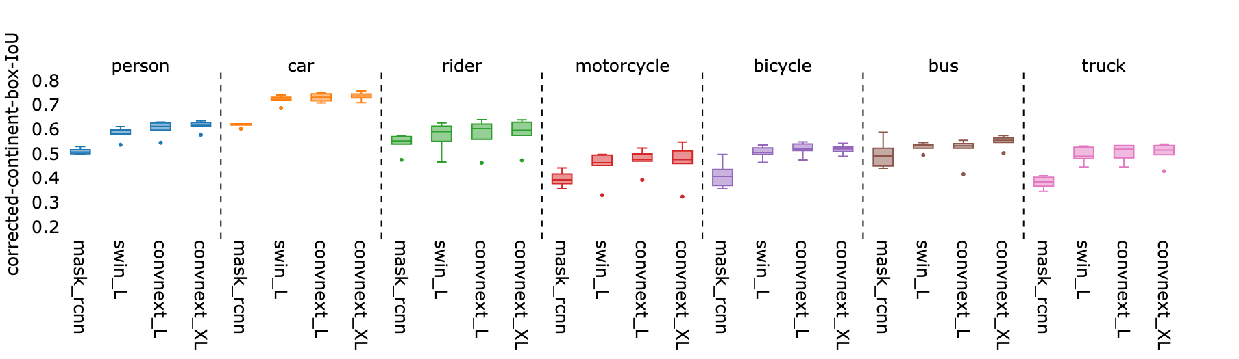
((a))

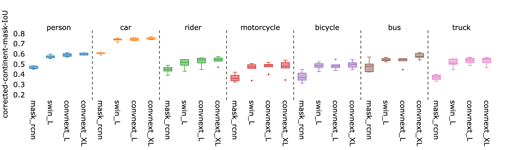
((b))

Figure 3: Detection and segmentation box plots after class-merging. Class-merging was applied to the following groups: car-bus-truck, motorcycle-bicycle, and person-rider.

3.2 Models

We used a total of four models in our experiments to ensure our findings are not limited to a single architecture. We used the Mask-RCNN model (with ResNet-50 backbone) since it is widely used for instance segmentation tasks. Given the growing popularity of vision transformers (ViTs), we also evaluated OneFormer, which is the current state-of-the-art ViT available for instance segmentation. We used Swin-L, ConvNext-L, and ConvNext-XL backbones for OneFormer. For all models, we examined geo-biases in segmentation performance (using instance masks) and detection performance (using bounding boxes of these instances). Using these models, we covered the two most widely used instance segmentation approaches: detect-and-segment (Mask-RCNN) and segment-only (OneFormer).

3.3 Datasets

We pre-trained all four models on the Cityscapes dataset [4]. Cityscapes is a widely used, Eurocentric driving dataset containing complex urban street scenes from cities in Germany and neighboring countries in Europe. The Cityscapes instance segmentation dataset has $3475$ images. The pre-trained model for Mask-RCNN was sourced from MMDetection [3], while the OneFormer models were sourced from the author’s GitHub repository [1].

We used Mapillary Vistas (Vistas) [12] for evaluating models trained on Cityscapes. To the best of our knowledge, Vistas is the only driving dataset with global coverage and instance-level annotations (refer to a comparison of different driving datasets in section A). Vistas is an instance segmentation dataset that was originally proposed to improve the geographic diversity of datasets like Cityscapes. Vistas contains $20,000$ (training and validation) images of street scenes on six continents (Europe, North America, South America, Africa, Asia, and Oceania).

Since the Vistas dataset does not include geographic metadata, we used the Mapillary API to obtain the longitude and latitude of each image. We removed images for which location metadata could not be obtained. We published the metadata, including Vistas image IDs and their corresponding latitude and longitude information on $<$anonymous link$>$.

We combined the training and validation sets into a single evaluation dataset for our experiments. We did not use the Vistas test set because it did not contain location metadata. Our resulting Vistas evaluation dataset contains $11,300$ images. We provide additional information about our Vistas evaluation dataset (number of images per continent, number of instances for each class in a continent) in section B.

We evaluated Eurocentric models trained on Cityscapes using geographically diverse images from Vistas to investigate geo-bias in Eurocentric models. To assess geo-bias, we measured model performance for each of the $6$ continents. We could not evaluate at the country level since certain countries (e.g., Uganda, Mozambique) had only one image in Vistas. We chose all classes common to both Cityscapes and Vistas: person, car, bus, truck, bicycle, motorcycle, and rider. Note that Vistas uses two classes — motorcyclist and bicyclist, instead of one rider class. To ensure consistent labels, we relabeled both classes in Vistas as the rider class.

For pre-processing, we filtered images in Vistas that had at least one of the classes in our study. Next, we resized these images such that the smaller side of each image was 1024 pixels. This resizing was done to match the resolution on which the Mask-RCNN was pre-trained. We used the same resolution while evaluating the ViT models for a fair comparison. We ignored point-like objects that occupied less than $0.01\%$ of pixels in the image. Point-like objects do not have shape or texture information. We would be unable to find concrete insights on geo-biases by analyzing them.

3.4 Metrics

Since we are the first study to examine geo-biases in instance segmentation, we discuss the appropriate metric to compare performance variations across geographies (in our case, continents).

In widely used datasets like Cityscapes and similar benchmarks, the Average Precision (AP) metric is used to evaluate instance segmentation models. AP is calculated across $10$ IoU (intersection-over-union) thresholds, ranging from $0.5$ to $0.95$ in steps of $0.05$. While AP is useful for comparing performance between different models, it may not be suitable for comparing the performance of a single model between different continents.

As an example, let us compare the performance of a Eurocentric model between two continents: Africa and Asia. Assume the Eurocentric model predicts an IoU in the range $(0,0.2)$ for all bus instances in Africa and $(0.25,0.45)$ for all bus instances in Asia. Although there is a disparity in IoUs between Africa and Asia, the bus-AP for both continents would be $0$ (as both precision and recall are $0$), indicating no performance disparity (or geo-bias). The AP metric penalizes bus predictions in both continents due to the high IoU threshold of $0.5$. While lowering the IoU threshold could address this issue, choosing a new threshold introduces human bias.

To eliminate external biases (e.g., human bias) from our geo-bias evaluations, we selected model predictions with the highest IoU (i.e., highest overlap) for the ground truth instances. We then averaged these IoU scores for each class. We ignored duplicate predictions of an instance, as they are not relevant when examining geo-biases. If the model failed to predict a ground truth instance, we assigned an IoU score of $0$ for that instance.

4 Results

4.1 Are Eurocentric models geo-biased?

In this study, we analyzed geo-biases in instance segmentation models at two levels of localization: detection and segmentation. We measured geo-biases in segmentation performance (using instance masks) and in detection performance (using bounding boxes for these instances).

First, we calculated the classwise performance of a model in each continent, which we call the continent-IoU:

$$\text{continent-IOU}_{C,y}(I,\hat{I})=\frac{1}{N_{C,y}}\sum_{k\in K}IOU(I_{k},\hat{I_{k}})$$ (1)

Here, $C$ represents a continent (e.g., Europe), and $y$ represents a class (e.g., person). $K$ refers to all instances of class $y$ in continent $C$. $I_{k}$ and $\hat{I_{k}}$ represent the ground-truth and predicted masks for the $k^{th}$ instance. $N_{C,y}$ represents the number of instances of class $y$ in continent $C$ .

Using this formula, we calculated continent-box-IoUs (for detection performance) and continent-mask-IoUs (for segmentation performance) for each {class, model} pair. Figure 2(a) and Figure 2(b) report box plots of continent-box-IoUs and continent-mask-IoUs, respectively. We used box plots because their interquartile ranges (boxes) effectively visualize the geo-biases in a {class, model} pair.

For detection performance, Figure 2(a) shows that the interquartile range (IQR) for the person (e.g., IQR for Swin-L $=0.014$) and car (e.g., IQR for Swin-L $=0.011$) box plots is small, regardless of the model. For the other five classes, we observed significantly larger IQRs across models. For example, with Swin-L, the IQR for trucks (IQR $=0.057$) is nearly $4\times$ that of the person class, and the IQR for buses (IQR $=0.085$) is nearly $7\times$ that of the person class.

For segmentation performance, the box plots in Figure 2(b) show a similar trend to those for detection in Figure 2(a). Overall, the results in Figures 2(a) and 2(b) indicate that Eurocentric models have minimal geo-biases for the person and car classes. However, they exhibit significant geo-biases for rider, motorcycle, bicycle, bus, and truck classes.

4.2 What types of errors are driving geo-bias?

For the classes that were geo-biased (rider, bus, truck, motorcycle, bicycle), Eurocentric models performed the worst in Africa and Asia. In Figure 4, we visualized some of the incorrect predictions made by the Swin-L on images from Africa and Asia.

As shown in the first two columns in Figure 4, the Swin-L often misclassified buses and trucks in Africa as cars. Mini-buses are a common mode of transportation in Africa that are less common in Western countries, where buses are typically larger. These mini-buses resemble large cars or vans in Europe, where they would likely be annotated with the car class. The Swin-L also frequently misclassified motorcycles in Africa and Asia as bicycles, as shown in the third column in Figure 4. This is because many motorcycles in Africa and Asia have thin wheels, visually similar to bicycles in Europe. Eurocentric models often confused objects in non-European continents (e.g., buses in Africa, motorcycles in Asia) with visually similar classes (e.g., cars, bicycles).

In a small number of cases, misclassifications occurred due to occlusion. For instance, when a bus was occluded, the model misclassified the bus as a car due to a lack of information. Such misclassifications occurred in buses as well as other classes like rider, motorcycle, and truck.

Figure 4: Misclassifications by a Eurocentric model (ViT-Swin-L) on images from Africa (left two) and Asia (right one). Objects circled in red were misclassified.

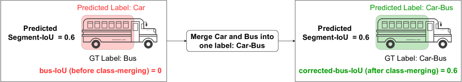
Figure 5: An example figure with a bus icon to demonstrate how class-merging resolves misclassification of the bus class and calculates a corrected-bus-IoU.

4.3 What is the contribution of classification error in geo-bias?

Since misclassifications were common in non-European continents, we measured their isolated contribution to geo-biases using a class-merging strategy. In class-merging, we merged classes that were visually similar (and often misclassified with each other) during evaluation.

As an example, assume that the bus icon shown in Figure 5 is originally labeled as a bus. Also, let us assume an instance segmentation model predicted a segment (or a bounding box) that has an IoU of $0.6$ with this bus. If the model mistakenly classified the bus as a car, the IoU of the bus class would be $0$. To address this misclassification, we modified the ground-truth class of the bus to car-bus. At the prediction stage, all car and bus predictions were also relabeled as car-bus. The bus that was previously predicted as a car is now predicted as the car-bus class. Since the ground-truth label matches the predicted label (car-bus), the model will return an IoU value of $0.6$ for car-bus. We remap this car-bus IoU value of $0.6$ back to the bus class. We refer to this updated IoU as the corrected-IoU of the bus class.

We applied class-merging on the following groups: car-bus-truck, motorcycle-bicycle and person-rider. These groupings were based on the general structure of objects. For instance, car-bus-truck contains $4$-wheeled vehicles, motorcycle-bicycle contains $2$-wheeled vehicles, and person-rider contains humans.

We applied class-merging to the detection and segmentation results and generated corrected-continent-box-IoUs and corrected-continent-mask-IoUs, respectively, for each class. Figure 3(a) and Figure 3(b) show the corrected-continent-box-IoUs and corrected-continent-mask-IoUs after class-merging.

Compared to Figures 2(a) and 2(b) (before class-merging), the IQR of the box plots in Figures 3(a) and 3(b) (after class-merging) were significantly reduced for the geo-biased classes (bus, motorcycle, bicycle, rider, and truck). In both detection and segmentation, class-merging significantly mitigated geo-bias.

To further demonstrate how class-merging mitigates geo-biases, we detailed the segmentation performance before and after class-merging of all classes for one of the segmentation models (Swin-L) in Table 1. The continent-mask-IoUs are shown on the left side of the arrow, while the corrected-continent-mask-IoUs are shown on the right side. As shown in Table 1, class-merging improved performance in non-European continents (especially Africa). This shows how misclassification contributed to performance drops in non-European continents.

Surprisingly, class-merging also improved the performance of Eurocentric models in Europe for classes like bus, truck, and rider. As discussed earlier, misclassifications can also occur when objects are occluded. Several of these occlusion cases were resolved in Europe through class-merging, which explains why the performance in Europe also increased after class-merging for some classes.

Table 1: Segmentation performance on ViT-Swin-L before (left) and after (right) class-merging. Values on the left of the arrow are continent-mask-IoUs, while values on the right are corrected-continent-mask-IoUs. Values highlighted in green indicate significant performance improvements ($>0.05$).

	Continents
Class	Europe	Africa	N. America	S. America	Asia	Oceania
person	$0.59\rightarrow 0.60$	$0.55\rightarrow 0.56$	$0.58\rightarrow 0.58$	$0.56\rightarrow 0.56$	$0.57\rightarrow 0.58$	$0.57\rightarrow 0.58$
car	$0.75\rightarrow 0.75$	$0.71\rightarrow 0.72$	$0.74\rightarrow 0.74$	$0.74\rightarrow 0.74$	$0.73\rightarrow 0.74$	$0.75\rightarrow 0.76$
bus
truck
bicycle	$0.46\rightarrow 0.47$	$0.51\rightarrow 0.51$	$0.49\rightarrow 0.50$	$0.52\rightarrow 0.52$	$0.42\rightarrow 0.43$	$0.46\rightarrow 0.47$
motorcycle	$0.46\rightarrow 0.46$		$0.47\rightarrow 0.50$	$0.44\rightarrow 0.47$	$0.45\rightarrow 0.48$	$0.49\rightarrow 0.51$
rider

Using the corrected-IoU scores (obtained through class-merging), we measured the contribution of classification errors in geo-bias. To measure this contribution, we first introduce a term to measure geo-biases in models, called geo-disparity. We define geo-disparity as the variation in model performance across continents. We calculated geo-disparity (Disp) using the ratio of the standard deviation in continent-IoUs (box or mask) to the mean continent-IoU for a {class, model} pair: $\text{Disp}=\sigma_{\text{continents}}/\mu_{\text{continents}}$. Normalizing geo-disparity by $\mu_{\text{continents}}$ ensures scale invariance.

To measure the contribution of classification errors in detection, we computed two measures: $\text{Disp}_{\text{det}}$, the disparity in detection performance originally (before class-merging), and $\text{Disp}_{\text{det-corrected}}$, the disparity in detection performance after class-merging. We computed the percentage change in disparity for detection performance before and after class-merging:

$$\text{Disp}_{\text{det-det-corrected}}=\frac{\text{Disp}_{\text{det-corrected}}-\text{Disp}_{\text{det}}}{\text{Disp}_{\text{det}}}\times 100$$ (2)

In the second column of Table 2, we show the $\text{Disp}_{\text{det-det-corrected}}$ (percentage change) values for each class for the Swin-L model. Class-merging reduced the geo-disparity in detection for all geo-biased classes: $19\%$ for bicycles, $36\%$ for motorcycles, $37\%$ for riders, $45\%$ for trucks, and $88\%$ for buses. This shows that classification errors accounted for $19$-$88\%$ of the geo-biases in detection performance. There were small changes in geo-disparity for the person and car classes as geo-biases were already negligible.

Similar to detection, we measured the contribution of classification errors in segmentation using the corresponding geo-disparity measures:

$$\text{Disp}_{\text{seg-seg-corrected}}=\frac{\text{Disp}_{\text{seg-corrected}}-\text{Disp}_{\text{seg}}}{\text{Disp}_{\text{seg}}}\times 100$$ (3)

In the third column of Table 2, we show the $\text{Disp}_{\text{seg-seg-corrected}}$ (percentage change) values for each class for the Swin-L model. Similar to detection, class-merging reduced the geo-disparity in segmentation for all geo-biased classes: $10\%$ for bicycles, $37\%$ for trucks, $39\%$ for motorcycles, $47\%$ for riders, and $90\%$ for buses. Hence, classification errors accounted for $10$-$90\%$ of the geo-biases in segmentation performance. As expected, there were minimal changes in geo-disparity for the person and car classes.

We observed similar reductions in geo-bias (in detection and segmentation) after class-merging for all the other instance segmentation models (Mask-RCNN, ConvNext-L, and ConvNext-XL). We provide the $\text{Disp}_{\text{det-det-corrected}}$ and the $\text{Disp}_{\text{seg-seg-corrected}}$ values for these models in Section C.

In conclusion, classification errors are the dominant source of geo-bias in instance segmentation models. For the geo-biased classes (bus, truck, bicycle, motorcycle, and rider), classification errors contributed to $19$-$88\%$ of the geo-biases in detection performance and $10$-$90\%$ of the geo-biases in segmentation performance.

Table 2: Percentage change in geo-disparity for the Swin-L. Column $2$ shows the change in disparity in detection performance before and after class-merging ($\text{Disp}_{\text{det-det-corrected}}$). Column $3$ shows the change in disparity in segmentation performance before and after class-merging ($\text{Disp}_{\text{seg-seg-corrected}}$).

Class	$\text{Disp}_{\text{det-det-corrected}}$	$\text{Disp}_{\text{seg-seg-corrected}}$
person	$-5.78\%$	$-5.32\%$
car	$6.07\%$	$0.61\%$
bus	$-88.68\%$	$-90.07\%$
truck	$-45.14\%$	$-37.59\%$
bicycle	$-19.44\%$	$-10.62\%$
motorcycle	$-36.29\%$	$-39.66\%$
rider	$-37.38\%$	$-47.44\%$

5 Discussion

In Section 4, we saw that geo-biases in Eurocentric models were primarily due to classification errors. Localization errors accounted for only a small part of geo-biases. We also observed that these models often misclassified objects from non-European regions. For example, small buses in Africa and motorcycles in Asia were frequently confused with visually similar objects in Europe, like cars and bicycles. A simple strategy like class-merging, which addressed these classification errors, reduced geo-biases in the geo-biased classes by up to $19$-$88\%$ in detection and $10$-$90\%$ in segmentation.

The classes we merged in our class-merging strategy (e.g., car-bus-truck, motorcycle-bicycle, and person-rider) shared similar structural features. For instance, car-bus-truck includes vehicles with $4+$ wheels, motorcycle-bicycle includes two-wheelers, and person-rider includes people. In essence, we created a coarser version of the original Vistas classes.

Our findings suggest that region-specific models, like Eurocentric ones, could perform better globally if coarser class labels are used. By simplifying class labels (e.g., four-wheeler over car vs. bus or two-wheeler over motorcycle vs. bicycle), we can reduce misclassifications and largely mitigate geo-biases. However, further research is needed to mitigate geo-biases arising from localization issues.

For applications where fine-grained class labels are important, other strategies may be more effective. We can train and test models within the same region (e.g., train on African data, test on African data). However, this approach is only feasible if sufficient training data is available for the target region (Africa in this example). We can also use geography-aware classification techniques [11] to reduce misclassifications and, consequently, geo-bias.

6 Limitations

Our study is the first to provide insights into geographic biases in driving datasets for instance segmentation. We evaluated Eurocentric models (trained on Cityscapes) using only one globally curated driving dataset: Mapillary Vistas. Although this might appear as a limitation, Vistas is the only publicly available driving dataset that offers global coverage and instance-level annotations, as detailed in Section A.

We used models pre-trained only on the Cityscapes (Eurocentric) dataset. For the driving datasets that supported instance segmentation (shown in Section A), the models we used only supported training on Cityscapes (Eurocentric dataset). Future work could focus on investigating geo-biases in Americentric datasets like BDD100k.

In our study, we examined seven classes that were common to both Cityscapes and Vistas. Most datasets (including Cityscapes and Vistas) typically provide instance-level annotations only for objects critical to driving safety, such as people, cars, and trucks. Several important classes that could have added value to this study (e.g., traffic signs and traffic lights) did not have instance-level annotations.

We also point out a limitation in our class-merging strategy. In class-merging, we manually identified classes that were visually similar and merged them during evaluation. Future research could explore ways to automate class-merging, perhaps using metrics that measure visual similarity among classes.

Although we provided country-level metadata for the Vistas images (as shown in Section 3.3), we examined geo-biases at the continent level. This is because some countries had very few images in the dataset. For instance, countries like Uganda and Mozambique (in Africa) had only one image each in Vistas. Since we examined geo-biases at the continent level, we could not capture performance variations between countries.

7 Conclusion

We investigated if instance segmentation models trained on Cityscapes (a Eurocentric driving dataset) are geo-biased. We used Vistas, a driving dataset with global coverage, to test the performance of Eurocentric models on driving scenes from new geographic regions.

We observed that geo-biases were present for some classes (bus, truck, motorcycle, bicycle, rider) but not for others (person, car). For most of the geo-biased classes, geo-biases were caused by classification errors, not localization errors. Eurocentric models often misclassified objects in non-European continents (e.g., buses in Africa, motorcycles in Asia) with visually similar objects in Europe (e.g., cars, bicycles). Using a class-merging strategy, we showed that for geo-biased classes, classification errors contributed to $19$-$88\%$ of the geo-biases in detection and $10$-$90\%$ of the geo-biases in segmentation. Hence, we identified that geo-biases are largely due to issues in classification rather than localization.

In class-merging, we created simpler, coarse-grained classes (e.g., four-wheelers, two-wheelers, and humans) for the original Vistas classes and mitigated geo-biases. Hence, region-specific models (Eurocentric in our case), when used globally, could benefit from coarser class definitions. However, this does not mitigate geo-biases stemming from localization errors. Although geo-biases from localization are minimal, mitigating these biases requires further research.

Supplementary Material

Appendix A Dataset Comparision

We compared some of the widely used driving datasets in Table 3. It is evident that Mapillary Vistas (Vistas) [12] is the only dataset with global coverage and instance-level annotations.

Appendix B Additional Details on Vistas

In Table 4, we show the number of images in each continent in Vistas. Note that the total count of images in Table 4 ($10,547$) is lesser than the number of images in our Vistas evaluation set ($11,300$ reported in Section 3.3). This is because a few images were eliminated in pre-processing (pre-processing steps are discussed in Section 3.3).

Table 5 shows the number of instances of each class in each continent. To compute Table 5, we used the $10,547$ images obtained after the pre-processing stage. Tables 4 and 5 confirm that we had sufficient instances across continents (for most classes) to conduct robust geo-bias evaluations.

Appendix C Class-merging on additional models

In addition to Swin-L (shown in Table 2), we applied class-merging on the following instance segmentation models: Mask-RCNN, ConvNext-L, and ConvNext-XL. Table 7 shows the $\text{Disp}_{\text{det-det-corrected}}$ and the $\text{Disp}_{\text{seg-seg-corrected}}$ values for these models. Similar to Swin-L, for the geo-biased classes, the geo-disparity in detection and segmentation performance reduced for all models (Mask-RCNN, ConvNext-L, ConvNext-XL) after class-merging. This shows that classification errors significantly contributed to geo-biases in instance segmentation models.

To further demonstrate that class-merging mitigates geo-biases in detection, we also applied class-merging to well-known object detection models (trained on Cityscapes): YOLOv7 and Faster-RCNN. Table 8 shows the $\text{Disp}_{\text{det-det-corrected}}$ values for these models. Similar to the segmentation models (shown in Tables 2 and 7), the geo-disparity in detection performance reduced for YOLOv7 and Faster-RCNN after class-merging.

Interestingly, in Faster-RCNN, the geo-disparity increased for buses ($32\%$) and slightly for motorcycles ($9\%$). To explain the increase in geo-disparity, we show the continent-box-IoUs for buses and motorcycles before and after class-merging in Table 6.

For buses, the detection performance of Faster-RCNN before class-merging was similar across continents. After class-merging, performance improved significantly in non-European continents like Africa ($0.36$ to $0.61$), North America ($0.30$ to $0.51$), and Oceania ($0.37$ to $0.54$), compared to a smaller improvement in Europe ($0.30$ to $0.43$). This led to an increase in geo-disparity. Similarly, for motorcycles, non-European continents like North America ($0.40$ to $0.45$), South America ($0.39$ to $0.48$), and Asia ($0.42$ to $0.46$) saw larger gains than Europe ($0.40$ to $0.42$).

Despite the increased geo-disparity in buses (and marginally in motorcycles) for Faster-RCNN, the results show that classification errors significantly impacted performance in non-European continents.

Table 3: A comparison of well-known driving datasets.

Driving Datasets	Continents Covered						Instance Segmentation
	Asia	Europe	N. America	S. America	Africa	Oceania
IDD [16]	✓	✗	✗	✗	✗	✗	✗
BDD100K [17]	✗	✗	✓	✗	✗	✗	✓
Cityscapes [4]	✗	✓	✗	✗	✗	✗	✓
nuScenes [2]	✓	✗	✓	✗	✗	✗	✓
ApolloScapes [8]	✓	✗	✗	✗	✗	✗	✗
Mapillary Vistas [12]	✓	✓	✓	✓	✓	✓	✓

Table 4: Number of images per continent in the Vistas dataset.

Continent	Asia	Europe	N. America	S. America	Africa	Oceania	Total
Number of Images	2157	3752	3090	712	154	682	10547

Table 5: Number of instances of each class in each continent in the Vistas dataset.

Class	Asia	Europe	N. America	S. America	Africa	Oceania
person	1892	10106	4265	2197	833	1109
car	9514	21848	22068	4820	1090	4256
bus	459	943	435	350	80	94
truck	1205	886	1057	275	84	165
bicycle	411	1691	380	160	24	69
motorcycle	743	1022	149	388	128	37
rider	771	1178	322	469	127	62

Table 6: Detection performance on Faster-RCNN for buses and motorcycles before and after class-merging. Values on the left of the arrow are continent-box-IoUs, while values on the right are corrected-continent-box-IoUs.

	Continents
Class	Europe	Africa	N. America	S. America	Asia	Oceania
bus	$0.30\rightarrow 0.43$	$0.36\rightarrow 0.61$	$0.30\rightarrow 0.51$	$0.33\rightarrow 0.49$	$0.29\rightarrow 0.44$	$0.37\rightarrow 0.54$
motorcycle	$0.40\rightarrow 0.42$	$0.36\rightarrow 0.43$	$0.40\rightarrow 0.45$	$0.39\rightarrow 0.48$	$0.42\rightarrow 0.46$	$0.37\rightarrow 0.40$

Table 7: Percentage change in geo-disparity for various instance segmentation models. Column $2$ shows the change in disparity in detection performance before and after class-merging ($\text{Disp}_{\text{det-det-corrected}}$). Column $3$ shows the change in disparity in segmentation performance before and after class-merging ($\text{Disp}_{\text{seg-seg-corrected}}$).

Model Name	Class	$\text{Disp}_{\text{det-det-corrected}}$	$\text{Disp}_{\text{seg-seg-corrected}}$
Mask-RCNN	person	$4.05\%$	$2.72\%$
	car	$-5.97\%$	$-6.97\%$
	bus	$-29.06\%$	$-29.18\%$
	truck	$-28.84\%$	$-24.96\%$
	bicycle	$-15.41\%$	$-11.45\%$
	motorcycle	$-26.83\%$	$-17.03\%$
	rider	$-15.64\%$	$-19.35\%$
ConvNext-L	person	$-0.65\%$	$1.34\%$
	car	$4.87\%$	$1.44\%$
	bus	$-66.61\%$	$-72.34\%$
	truck	$-29.97\%$	$-42.22\%$
	bicycle	$-7.99\%$	$-1.10\%$
	motorcycle	$-30.42\%$	$-40.02\%$
	rider	$-34.12\%$	$-46.19\%$
ConvNext-XL	person	$-2.76\%$	$-0.23\%$
	car	$-10.43\%$	$-14.04\%$
	bus	$-74.10\%$	$-72.78\%$
	truck	$-29.14\%$	$-34.48\%$
	bicycle	$-16.60\%$	$-3.39\%$
	motorcycle	$-30.96\%$	$-37.36\%$
	rider	$-27.12\%$	$-44.82\%$

Table 8: Percentage change in geo-disparity for various detection models. Column $2$ shows the change in disparity in detection performance before and after class-merging ($\text{Disp}_{\text{det-det-corrected}}$)

. Model Name Class $\text{Disp}_{\text{det-det-corrected}}$ YOLOv7 person $-5.81\%$ car $2.59\%$ bus $-55.49\%$ truck $-34.21\%$ bicycle $-0.47\%$ motorcycle $-33.13\%$ rider $-14.23\%$ Faster-RCNN person $-2.66\%$ car $-6.46\%$ bus $32.55\%$ truck $-51.98\%$ bicycle $-1.85\%$ motorcycle $9.41\%$ rider $-6.79\%$

References

- one [2023] https://github.com/SHI-Labs/OneFormer, 2023.
- Caesar et al. [2020] Holger Caesar, Varun Bankiti, Alex H Lang, Sourabh Vora, Venice Erin Liong, Qiang Xu, Anush Krishnan, Yu Pan, Giancarlo Baldan, and Oscar Beijbom. nuscenes: A multimodal dataset for autonomous driving. In Proceedings of the IEEE/CVF conference on computer vision and pattern recognition, pages 11621–11631, 2020.
- Chen et al. [2019] Kai Chen, Jiaqi Wang, Jiangmiao Pang, Yuhang Cao, Yu Xiong, Xiaoxiao Li, Shuyang Sun, Wansen Feng, Ziwei Liu, Jiarui Xu, et al. Mmdetection: Open mmlab detection toolbox and benchmark. arXiv preprint arXiv:1906.07155, 2019.
- Cordts et al. [2016] Marius Cordts, Mohamed Omran, Sebastian Ramos, Timo Rehfeld, Markus Enzweiler, Rodrigo Benenson, Uwe Franke, Stefan Roth, and Bernt Schiele. The cityscapes dataset for semantic urban scene understanding. In Proceedings of the IEEE conference on computer vision and pattern recognition, pages 3213–3223, 2016.
- De Vries et al. [2019] Terrance De Vries, Ishan Misra, Changhan Wang, and Laurens Van der Maaten. Does object recognition work for everyone? In Proceedings of the IEEE/CVF Conference on Computer Vision and Pattern Recognition Workshops, pages 52–59, 2019.
- Deng et al. [2009] Jia Deng, Wei Dong, Richard Socher, Li-Jia Li, Kai Li, and Li Fei-Fei. Imagenet: A large-scale hierarchical image database. In 2009 IEEE conference on computer vision and pattern recognition, pages 248–255. Ieee, 2009.
- Gustafson et al. [2024] Laura Gustafson, Megan Richards, Melissa Hall, Caner Hazirbas, Diane Bouchacourt, and Mark Ibrahim. Exploring why object recognition performance degrades across income levels and geographies with factor annotations. Advances in Neural Information Processing Systems, 36, 2024.
- Huang et al. [2018] Xinyu Huang, Xinjing Cheng, Qichuan Geng, Binbin Cao, Dingfu Zhou, Peng Wang, Yuanqing Lin, and Ruigang Yang. The apolloscape dataset for autonomous driving. In Proceedings of the IEEE conference on computer vision and pattern recognition workshops, pages 954–960, 2018.
- Kalluri et al. [2023] Tarun Kalluri, Wangdong Xu, and Manmohan Chandraker. Geonet: Benchmarking unsupervised adaptation across geographies. In Proceedings of the IEEE/CVF Conference on Computer Vision and Pattern Recognition, pages 15368–15379, 2023.
- Kuznetsova et al. [2020] Alina Kuznetsova, Hassan Rom, Neil Alldrin, Jasper Uijlings, Ivan Krasin, Jordi Pont-Tuset, Shahab Kamali, Stefan Popov, Matteo Malloci, Alexander Kolesnikov, et al. The open images dataset v4: Unified image classification, object detection, and visual relationship detection at scale. International Journal of Computer Vision, 128(7):1956–1981, 2020.
- Mac Aodha et al. [2019] Oisin Mac Aodha, Elijah Cole, and Pietro Perona. Presence-only geographical priors for fine-grained image classification. In Proceedings of the IEEE/CVF International Conference on Computer Vision, pages 9596–9606, 2019.
- Neuhold et al. [2017] Gerhard Neuhold, Tobias Ollmann, Samuel Rota Bulo, and Peter Kontschieder. The mapillary vistas dataset for semantic understanding of street scenes. In Proceedings of the IEEE International Conference on Computer Vision, pages 4990–4999, 2017.
- Ramaswamy et al. [2023] Vikram V Ramaswamy, Sing Yu Lin, Dora Zhao, Aaron Bryan Adcock, Laurens van der Maaten, Deepti Ghadiyaram, and Olga Russakovsky. Geode: a geographically diverse evaluation dataset for object recognition. In Thirty-seventh Conference on Neural Information Processing Systems Datasets and Benchmarks Track, 2023.
- Rojas et al. [2022] William A Gaviria Rojas, Sudnya Diamos, Keertan Ranjan Kini, David Kanter, Vijay Janapa Reddi, and Cody Coleman. The dollar street dataset: Images representing the geographic and socioeconomic diversity of the world. In Thirty-sixth Conference on Neural Information Processing Systems Datasets and Benchmarks Track, 2022.
- Shankar et al. [2017] Shreya Shankar, Yoni Halpern, Eric Breck, James Atwood, Jimbo Wilson, and D Sculley. No classification without representation: Assessing geodiversity issues in open data sets for the developing world. arXiv preprint arXiv:1711.08536, 2017.
- Varma et al. [2019] Girish Varma, Anbumani Subramanian, Anoop Namboodiri, Manmohan Chandraker, and CV Jawahar. Idd: A dataset for exploring problems of autonomous navigation in unconstrained environments. In 2019 IEEE Winter Conference on Applications of Computer Vision (WACV), pages 1743–1751. IEEE, 2019.
- Yu et al. [2020] Fisher Yu, Haofeng Chen, Xin Wang, Wenqi Xian, Yingying Chen, Fangchen Liu, Vashisht Madhavan, and Trevor Darrell. Bdd100k: A diverse driving dataset for heterogeneous multitask learning. In Proceedings of the IEEE/CVF conference on computer vision and pattern recognition, pages 2636–2645, 2020.