DisCo-DSO: Coupling Discrete and Continuous Optimization for Efficient Generative Design in Hybrid Spaces

Abstract

We consider the challenge of black-box optimization within hybrid discrete-continuous and variable-length spaces, a problem that arises in various applications, such as decision tree learning and symbolic regression. We propose DisCo-DSO (Discrete-Continuous Deep Symbolic Optimization), a novel approach that uses a generative model to learn a joint distribution over discrete and continuous design variables to sample new hybrid designs. In contrast to standard decoupled approaches, in which the discrete and continuous variables are optimized separately, our joint optimization approach uses fewer objective function evaluations, is robust against non-differentiable objectives, and learns from prior samples to guide the search, leading to significant improvement in performance and sample efficiency. Our experiments on a diverse set of optimization tasks demonstrate that the advantages of DisCo-DSO become increasingly evident as the complexity of the problem increases. In particular, we illustrate DisCo-DSO’s superiority over the state-of-the-art methods for interpretable reinforcement learning with decision trees.

Introduction

(a) Standard decoupled approach

(b) DisCo-DSO

Figure 1: Comparison of the standard decoupled approach and DisCo-DSO for discrete-continuous optimization using an autoregressive model. In the decoupled approach, the discrete skeleton $\tau_{\text{d}}=\langle(l_{1},\cdot),\ldots,(l_{T},\cdot)\rangle$ is sampled first and then the continuous parameters $\beta_{1},\ldots,\beta_{T}$ are optimized independently. In contrast, DisCo-DSO models the joint distribution over the sequence of tokens $\langle(l_{1},\beta_{1}),\ldots,(l_{T},\beta_{T})\rangle$. Here, the notation $\oplus$ stands for concatenation of vectors.

Deep learning methods have shown success in important combinatorial optimization problems (Bello et al., 2016), including generating interpretable policies for continuous control (Landajuela et al., 2021b) and symbolic regression (SR) to discover the underlying mathematical equations from the data (Petersen et al., 2021a; Biggio et al., 2021; Kamienny et al., 2022; Landajuela et al., 2022). Existing approaches train a generative model that constructs a solution to the optimization problem by sequentially choosing from a set of discrete tokens, using the value of the objective function as the terminal reward for learning. However, these approaches do not jointly optimize the discrete and continuous components of such hybrid problems: Certain discrete tokens require the additional specification of an associated real-valued parameter, such as the threshold value at a decision tree node or the value of a constant token in an equation, but the learned generative model does not produce these values. Instead, they adopt the design choice of decoupled optimization, whereby only the construction of a discrete solution skeleton is optimized by deep learning, while the associated continuous parameters are left to a separate black-box optimizer.

We hypothesize that a joint discrete-continuous optimization approach (Figure 1(b)) that generates a complete solution based on deep reinforcement learning (RL) (Sutton and Barto, 2018) has significant advantages compared to existing decoupled approaches that employ learning only for the discrete skeleton (Figure 1(a)). In terms of efficiency, a joint approach only requires one evaluation of the objective function for each candidate solution, whereas the decoupled approach based on common non-linear black-box optimization methods such as BFGS (Fletcher, 2000), simulated annealing (Xiang et al., 1997), or evolutionary algorithms (Storn and Price, 1997) requires a significant number of function evaluations to optimize each discrete skeleton. This decoupled approach incurs a high cost for applications such as interpretable control, where each objective function evaluation involves running the candidate solution on many episodes of a high-dimensional and stochastic physical simulation (Landajuela et al., 2021b). Furthermore, joint exploration and learning on the full discrete-continuous solution space has the potential to escape from local optima and use information from prior samples to guide the subsequent search.

In this work, we consider discrete-continuous optimization problems that exhibit several key distinguishing features: (1) a black-box reward, (2) a variable-length structure of the design space, and (3) a sequential structure in the form of prefix-dependent positional constraints. These problems are not well-suited to existing joint optimization approaches such as Mixed Integer Programming (MIP) (Fischetti and Jo, 2018; Nair et al., 2021) or Mixed Bayesian Optimization (BO) (Daxberger et al., 2019), which are designed for problems with fixed-length discrete components and do not naturally handle positional constraints in the design space. To address these challenges, we draw upon the success of deep reinforcement learning in parameterized action space Markov decision processes (Hausknecht and Stone, 2016) to extend existing deep learning methods for discrete optimization (Bello et al., 2016; Zoph and Le, 2017; Petersen et al., 2021a; Landajuela et al., 2021b) to the broader space of joint discrete-continuous optimization. We summarize the main contributions of this paper as follows:

• We propose a novel method for joint discrete-continuous optimization using autoregressive models and deep reinforcement learning, which we call DisCo-DSO, that is suited for black-box hybrid optimization problems over variable-length search spaces with prefix-dependent positional constraints.

• We present a novel formulation for decision tree policy search in control tasks as sequential discrete-continuous optimization and propose a method for sequentially finding bounds for parameter ranges in decision nodes.

• We perform exhaustive empirical evaluation of DisCo-DSO on a diverse set of tasks, including interpretable control policies and symbolic regression. We show that DisCo-DSO outperforms decoupled approaches on all tasks.

Related work

Hybrid discrete-continuous action spaces in reinforcement learning.

The treatment of the continuous parameters as part of the action space has strong parallels in the space of hybrid discrete-continuous RL. In Hausknecht and Stone (2016), the authors present a successful application of deep reinforcement learning to a domain with continuous state and action spaces. In Xiong et al. (2018), the authors take an off-policy DQN-type approach that directly works on the hybrid action space without approximation of the continuous part or relaxation of the discrete part, but requires an extra loss function for the continuous actions. In Neunert et al. (2020), they propose a hybrid RL algorithm that uses continuous policies for discrete action selection and discrete policies for continuous action selection.

Symbolic regression with constants optimization.

In the field of symbolic regression, different approaches have been proposed for addressing the optimization of both discrete skeletons and continuous parameters. Traditional genetic programming approaches and deep generative models handle these problems separately, with continuous constants optimized after discrete parameters (Topchy et al., 2001; Petersen et al., 2021a; Biggio et al., 2021). Recent works aim to jointly optimize discrete constants and continuous parameters by relaxing the discrete problem into a continuous one (Martius and Lampert, 2016; Sahoo et al., 2018), or by tokenizing (i.e., discretizing) the continuous constants (Kamienny et al., 2022). The former approach faces challenges such as exploding gradients and the need to revert continuous values to discrete ones. The latter approach tokenizes continuous constants, treating them similarly to discrete tokens, but such quantization is problem-dependent, restricts the search space, and requires additional post-hoc optimization to refine the continuous parameters.

Decision tree policies in reinforcement learning.

In the domain of symbolic reinforcement learning, where the goal is to find intelligible and concise control policies, works such as Landajuela et al. (2021b) and Sahoo et al. (2018) have discretized the continuous space and used relaxation approaches, respectively, to optimize symbolic control policies in continuous action spaces. For discrete action spaces, a natural representation of a symbolic policy is a decision tree (Ding et al., 2020; Silva et al., 2020; Custode and Iacca, 2023). In Custode and Iacca (2023), the authors use an evolutionary search to find the best decision tree policy and further optimized the real valued thresholds using a decoupled approach. Relaxation approaches find their counterparts within this domain in works such as Sahoo et al. (2018); Silva et al. (2020); Ding et al. (2020), where a soft decision tree is used to represent the policy. The soft decision tree, which fixes the discrete structure of the policy and exposes the continuous parameters, is then optimized using gradient-based methods.

Discrete-Continuous Deep Symbolic Optimization

Notation and problem definition

We consider a discrete-continuous optimization problem defined over a search space $\mathcal{T}$ of sequences of tokens $\tau=\langle\tau_{1},\ldots,\tau_{T}\rangle$, where each token $\tau_{i}$ belongs to a library $\mathcal{L}$ and the length $T$ of the sequence is not fixed a priori. The library $\mathcal{L}$ is a set of $K$ tokens $\mathcal{L}=\{l_{1},\ldots,l_{K}\}$, where a subset $\hat{\mathcal{L}}\subseteq\mathcal{L}$ of them are parametrized by a continuous parameter, i.e., each token $l\in\hat{\mathcal{L}}$ has an associated continuous parameter $\beta\in\mathcal{A}(l)\subset\mathbb{R}$, where $\mathcal{A}(l)$ is the token-dependent range. To ease the notation, we define $\bar{\mathcal{L}}\overset{\text{\tiny def}}{=}\mathcal{L}\setminus\hat{\mathcal{L}}$ and consider a dummy range $\mathcal{A}(l)=[0,1]\subset\mathbb{R}$ for the strictly discrete tokens $l\in\bar{\mathcal{L}}$. Thus, we define

$$l(\beta)=\begin{cases}l&\text{if }l\in\bar{\mathcal{L}}\\ l(\beta)&\text{if }l\in\hat{\mathcal{L}}\end{cases},\forall(l,\beta)\in\mathcal{L}\times\mathcal{A}(l).$$

In other words, the parameter $\beta$ is ignored if $l\in\bar{\mathcal{L}}$. With this notation, we can write $\tau_{i}=l_{i}(\beta_{i})\in\mathcal{L},\forall i\in\{1,\ldots,T\}$. In the following, we use the notation $l_{i}(\beta_{i})\equiv(l_{i},\beta_{i})$ and write $\tau=\langle\tau_{1},\ldots,\tau_{T}\rangle=\langle l_{1}(\beta_{1}),\ldots,l_{T}(\beta_{T})\rangle\equiv\langle(l_{1},\beta_{1}),\ldots,(l_{T},\beta_{T})\rangle.$

Given a sequence $\tau$, we define the discrete skeleton $\tau_{\text{d}}$ as the sequence obtained by removing the continuous parameters from $\tau$, i.e., $\tau_{\text{d}}=\langle(l_{1},\cdot),\ldots,(l_{T},\cdot)\rangle.$ We introduce the operator ${\tt eval}:\mathcal{T}\rightarrow\mathbb{T}$ to represent the semantic interpretation of the sequence $\tau$ as an object in the relevant design space $\mathbb{T}$. We consider problems with prefix-dependent positional constraints, i.e., problems for which, given a prefix $\tau_{1:(i-1)}$, there exists a possible non-empty set of unfeasible tokens $\mathcal{C}_{\tau_{1:(i-1)}}\subseteq\mathcal{L}$ such that ${\tt eval}(\tau_{1:(i-1)}\cup\tau_{i}\cup\tau_{(i+1):T})\notin\mathbb{T}$ for all $\tau_{i}\in\mathcal{C}_{\tau_{1:(i-1)}}$ and for all $\tau_{j}\in\mathcal{L}$ with $i<j\leq T$. Variable-length problems exhibiting such constraints are not well-suited for MIP solvers or classical Bayesian Optimization methods.

The optimization problem is defined by the reward function $R:\mathbb{T}\rightarrow\mathbb{R}$, which can be deterministic or stochastic. In the stochastic case, we have a reward distribution $p_{R}(r|t)$ conditioned on the design $t\in\mathbb{T}$ and the reward function is given by $R(t)=\mathbb{E}_{r\sim p_{R}(r|t)}[r].$ Note that we do not assume that the reward function $R$ is differentiable with respect to the continuous parameters $\beta_{i}$. In the following, we make a slight abuse of notation and use $R(\tau)$ and $p_{R}(r|\tau)$ to denote $R({\tt eval}(\tau))$ and $p_{R}(r|{\tt eval}(\tau))$, respectively. The optimization problem is to find a sequence $\tau^{*}=\langle\tau^{*}_{1},\ldots,\tau^{*}_{T}\rangle=\langle(l^{*}_{1},\beta^{*}_{1}),\ldots,(l^{*}_{T},\beta^{*}_{T})\rangle$ (where the length $T$ is not fixed a priori) such that $\tau^{*}\in\operatorname*{arg\,max}_{\tau\in\mathcal{T}}R(\tau)$.

Method

Combinatorial optimization with autoregressive models.

In applications of deep learning to combinatorial optimization (Bello et al., 2016), a probabilistic model $p(\tau)$ is learned over the design space $\mathcal{T}$. The model is trained to gradually allocate more probability mass to high scoring solutions. The training can be done using supervised learning, if problem instances with their corresponding solutions are available, or, more generally, using RL. In most cases, the model $p(\tau)$ is parameterized by an autoregressive (AR) model with parameters $\theta$. The model is used to generate sequences as follows.

At position $i$, the model emits a vector of logits $\psi^{(i)}$ conditioned on the previously generated tokens $\tau_{1:(i-1)}$, i.e., $\psi^{(i)}=\text{AR}(\tau_{1:(i-1)};\theta)$. The new token $\tau_{i}$ is sampled from the distribution $p(\tau_{i}|\tau_{1:(i-1)},\theta)=\text{softmax}(\psi^{(i)})_{\mathcal{L}(\tau_{i})},$ where $\mathcal{L}(\tau_{i})$ is the index in $\mathcal{L}$ corresponding to node value $\tau_{i}$. The new token $\tau_{i}$ is then added to the sequence $\tau_{1:(i-1)}$ and used to condition the generation of the next token $\tau_{i+1}$. The process continues until a stopping criterion is met.

Different model architectures can be employed to generate the logits $\psi^{(i)}$. For instance, recurrent neural networks (RNNs) have been utilized in Petersen et al. (2021a); Landajuela et al. (2021b); Mundhenk et al. (2021); da Silva et al. (2023), and transformers with causal attention have been applied in works like Biggio et al. (2021) and Kamienny et al. (2022).

Prefix-dependent positional constraints.

Sequential token generation enables flexible configurations and the incorporation of constraints during the search process (Petersen et al., 2021a). Specifically, given a prefix $\tau_{1:(i-1)}$, a prior $\psi^{(i)}_{\circ}\in\mathbb{R}^{|\mathcal{L}|}$ is computed such that ${\psi^{(i)}_{\circ}}_{\mathcal{L}(\tau_{i})}=-\infty$ for tokens $\tau_{i}$ in the unfeasible set $\mathcal{C}_{\tau_{1:(i-1)}}$ and zero otherwise. The prior is added to the logits $\psi^{(i)}$ before sampling the token $\tau_{i}$.

Extension to discrete-continuous optimization.

Current deep learning approaches for combinatorial optimization only support discrete tokens, i.e., $\hat{\mathcal{L}}=\emptyset$, (Bello et al., 2016) or completely decouple the discrete and continuous parts of the problem, as in Petersen et al. (2021a); Landajuela et al. (2021b); Mundhenk et al. (2021); da Silva et al. (2023), by sampling first the discrete skeleton $\tau_{\text{d}}$ and then optimizing its continuous parameters separately (see Figure 1(a)). In this work, we extend these frameworks to support joint optimization of discrete and continuous tokens. The model is extended to emit two outputs $\psi^{(i)}$ and $\phi^{(i)}$ for each token $\tau_{i}=(l_{i},\beta_{i})$ conditioned on the previously generated tokens, i.e., $\left(\psi^{(i)},\phi^{(i)}\right)=\text{AR}((l,\beta)_{1:(i-1)};\theta)$, where we use the notation $(l,\beta)_{1:(i-1)}$ to denote the sequence of tokens $\langle(l_{1},\beta_{1}),\ldots,(l_{i-1},\beta_{i-1})\rangle$ (see Figure 1(b)). Given tokens $(l,\beta)_{1:(i-1)}$, the $i^{\textrm{\tiny th}}$ token $(l_{i},\beta_{i})$ is generated by sampling from the following distribution:

$$p((l_{i},\beta_{i})|(l,\beta)_{1:(i-1)},\theta)=\begin{cases}\mathcal{U}_{[0,1]}(\beta_{i})\text{softmax}(\psi^{(i)})_{\mathcal{L}(l_{i})}&\text{if }l_{i}\in\bar{\mathcal{L}}\\ \mathcal{D}(\beta_{i}|l_{i},\phi^{(i)})\text{softmax}(\psi^{(i)})_{\mathcal{L}(l_{i})}&\text{if }l_{i}\in\hat{\mathcal{L}}\\ \end{cases},$$

where $\mathcal{D}(\beta_{i}|l_{i},\phi^{(i)})$ is the probability density function of the distribution $\mathcal{D}$ that is used to sample $\beta_{i}$ from $\phi^{(i)}$. Note that the choice of $\beta_{i}$ is conditioned on the choice of discrete token $l_{i}$. We assume that the support of $\mathcal{D}(\beta|l,\phi)$ is a subset of $\mathcal{A}(l)$ for all $l\in\hat{\mathcal{L}}$. Additional priors of the form $(\psi^{(i)}_{\circ},0)$ can be added to the logits before sampling the token $\tau_{i}$.

Training DisCo-DSO.

The parameters $\theta$ of the model are learned by maximizing the expected reward $J(\theta)=\mathbb{E}_{\tau\sim p(\tau|\theta)}[R(\tau)]$ or, alternatively, the quantile-conditioned expected reward $J_{\varepsilon}(\theta)=\mathbb{E}_{\tau\sim p(\tau|\theta)}[R(\tau)|R(\tau)\geq R_{\varepsilon}(\theta)],$ where $R_{\varepsilon}(\theta)$ represents the $(1-\varepsilon)$-quantile of the reward distribution $R(\tau)$ sampled from the trajectory distribution $p(\tau|\theta)$. The motivation for using $J_{\varepsilon}(\theta)$ is to encourage the model to focus on best case performance over average case performance (see Petersen et al. (2021a)), which is the preferred behavior in optimization problems. It is worth noting that both objectives, $J(\theta)$ and $J_{\varepsilon}(\theta)$, serve as relaxations of the original $\operatorname*{arg\,max}R(\tau)$ optimization problem described above.

To optimize the objective $J_{\varepsilon}(\theta)$, we extend the risk-seeking policy gradient of Petersen et al. (2021a) to the discrete-continuous setting. The gradient of $J_{\varepsilon}(\theta)$ reads as

$$\nabla_{\theta}J_{\varepsilon}(\theta)=\mathbb{E}_{\tau\sim p(\tau|\theta)}\left[A(\tau,\varepsilon,\theta)\,S((l,\beta)_{1:T})\mid A(\tau,\varepsilon,\theta)>0\right],$$

where $A(\tau,\varepsilon,\theta)=R(\tau)-R_{\varepsilon}(\theta)$ and

$$S((l,\beta)_{1:T})=\displaystyle\sum_{i=1}^{T}\begin{cases}\nabla_{\theta}\log p(l_{i}|(l,\beta)_{1:(i-1)},\theta)&\text{if }l_{i}\in\bar{\mathcal{L}},\\[8.61108pt] \begin{aligned} &\nabla_{\theta}\log p(l_{i}|(l,\beta)_{1:(i-1)},\theta)\\ &\ \ \ \ \ \ \ \ +\nabla_{\theta}\log p(\beta_{i}|l_{1:i},\beta_{1:i-1},\theta)\end{aligned}&\text{if }l_{i}\in\hat{\mathcal{L}}.\end{cases}$$

We provide pseudocode for DisCo-DSO, a derivation of the risk-seeking policy gradient, and additional details of the learning procedure in the appendix.

Experiments

We demonstrate the benefits and generality of our approach on a diverse set of tasks as follows. Firstly, we introduce a new pedagogical task, called Parameterized Bitstring, to understand the conditions under which the benefits of DisCo-DSO versus decoupled approaches become apparent. We then consider two preeminent tasks in combinatorial optimization: decision tree policy optimization for reinforcement learning and symbolic regression for equation discovery.

Baselines.

To demonstrate the advantages of joint discrete-continuous optimization, we compare DisCo-DSO with the following classes of methods:

• Decoupled-RL-{BFGS, anneal, evo}: This baseline trains a generative model with reinforcement learning to produce a discrete skeleton (Petersen et al., 2021a), which is then optimized by a downstream nonlinear solver for the continuous parameters. The objective value at the optimized solution is the reward, which is used to update the generative model using the same policy gradient approach and architecture as DisCo-DSO. The continuous optimizer is either L-BFGS-B (BFGS), simulated annealing (anneal) (Xiang et al., 1997), or differential evolution (evo) (Storn and Price, 1997), using the SciPy implementation (Virtanen et al., 2020).

• Decoupled-GP-{BFGS, anneal, evo}: This baseline uses genetic programming (GP) (Koza, 1990) to produce a discrete skeleton, which is then optimized by a downstream nonlinear solver for the continuous parameters.

• BO: For the Parameterized Bitstring task, which has a fixed length search space and no positional constraints, we also consider a Bayesian Optimization baseline using expected improvement as acquisition function (Shahriari et al., 2015; Garrido-Merchán and Hernández-Lobato, 2020).

All experiments involving RL and DisCo-DSO use a RNN with a single hidden layer of 32 units as the generative model. The GP baselines use the “Distributed Evolutionary Algorithms in Python” software (Fortin et al., 2012). Additional details are provided in the appendix.

Note on baselines for symbolic regression.

In the context of symbolic regression, some of the above baselines corresponds to popular methods in the literature. Specifically, Decoupled-RL-BFGS corresponds exactly to the method “Deep Symbolic Regression” from Petersen et al. (2021a), and Decoupled-GP-BFGS corresponds to a standard implementation of genetic programming for symbolic regression à la Koza (1994) (most common approach to symbolic regression in the literature).

Parameterized bitstring task

Problem formulation.

We design a general and flexible Parameterized Bitstring benchmark problem, denoted $\text{PB}(N,f,l^{*},\beta^{*})$, to test the hypothesis that DisCo-DSO is more efficient than the decoupled optimization approach. In each problem instance, the task is to recover a hidden string $l^{*}\in[0,1]^{T}$ of $T$ bits and a vector of parameters $\beta^{*}\in\mathbb{R}^{T}$. Each bit $l^{*}_{i}$ is paired with a parameter $\beta^{*}_{i}$ via the reward function $R$, which gives a positive value based on an objective function $f(\beta_{i},\beta^{*}_{i})\in[0,1]$ only if the correct bit $l_{i}^{*}$ is chosen at position $i$:

$$R(\tau,\beta)\overset{\text{\tiny def}}{=}\frac{1}{T}\sum_{i=1}^{T}\bm{1}_{\tau_{i}=\tau^{*}_{i}}\left(\alpha+(1-\alpha)f(\beta_{i},\beta^{*}_{i})\right)$$ (1)

The scalar $\alpha\in[0,1]$ controls the relative importance of expending computational effort to optimize the discrete or continuous parts of the reward. The problem difficulty can be controlled by increasing the length $T$ and increasing the nonlinearity of the objective function $f$, such as by increasing the number of local optima. In our experiment, we tested the following objective functions, which represent objectives with multiple suboptimal local maxima ($f_{1}$) and discontinuous objective landscapes ($f_{2}$):

$$f_{1}(x,x^{*})\overset{\text{\tiny def}}{=}\left\lvert\frac{\sin(50(x-x^{*}))}{50(x-x^{*})}\right\rvert,\quad\quad$$ (2)

$$f_{2}(x,x^{*})\overset{\text{\tiny def}}{=}\begin{cases}1,\quad&|x-x^{*}|\leq 0.05\\ 0.5,\quad&0.05<|x-x^{*}|\leq 0.1\\ 0,\quad&0.1<|x-x^{*}|\end{cases}.$$ (3)

Results.

Figure 2 shows that DisCo-DSO is significantly more sample efficient than the decoupled approach when the discrete solution contributes more to the overall reward. This is because each sample generated by DisCo-DSO is a complete solution, which costs only one function evaluation to get a reward. In contrast, each sample generated by the baseline decoupled methods only has a discrete skeleton, which requires many function evaluations using the downstream optimizer to get a single complete solution. As the discrete skeleton increases in importance, the relative contribution of function evaluations for continuous optimization decreases. Note that, given the same computational budget, the BO method performs less function evaluations than the rest of the methods and the final results are worse than DisCo-DSO. This is because BO has a computational complexity of $\mathcal{O}(n^{3})$ (Shahriari et al., 2015), where $n$ is the number of function evaluations. This computational complexity makes BO challenging or even infeasible for large $n$ (Lan et al., 2022).

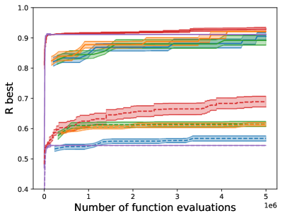
(a) Parameterized Bitstring with $f_{1}$

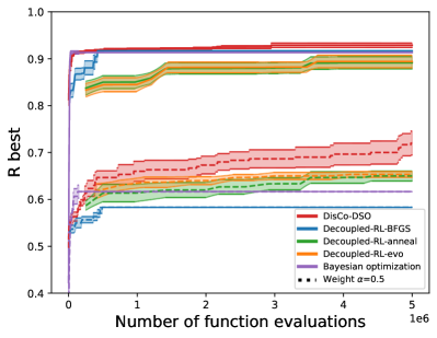
(b) Parameterized Bitstring with $f_{2}$

Figure 2: Reward of best solution versus number of function evaluations on a parameterized bitstring task, for two continuous optimization landscapes $f_{1}$ and $f_{2}$ and weights $\alpha=0.5,0.9$. Solid line corresponds to weight $\alpha=0.9$, dashed line $\alpha=0.5$. Mean and standard error over 5 seeds.

Decision tree policies for reinforcement learning

Problem formulation.

In this section we consider the problem of discovering decision tree policies for RL. We consider $\mathbb{T}$ as the space of univariate decision trees (Silva et al., 2020). Extensions to multivariate decision trees, also known as oblique trees, are possible, but we leave them for future work. Given an RL environment with observations $x_{1},\dots,x_{n}$ and discrete actions $a_{1},\dots,a_{m}$, we consider the library of Boolean expressions and actions given by $\mathcal{L}=\{x_{1}<\beta_{1},\dots,x_{n}<\beta_{n},a_{1},\dots,a_{m}\},$ where $\beta_{1},\dots,\beta_{n}$ are the values of the observations that are used in the internal nodes of the decision tree. The evaluation operator ${\tt eval}:\mathcal{T}\rightarrow\mathbb{T}$ is defined as follows. We treat sequence $\tau$ as the pre-order traversal of a decision tree, where the decision tokens ($x_{n}<\beta_{n}$) are treated as binary nodes and the action tokens ($a_{n}$) are treated as leaf nodes. For evaluating the decision tree, we start from the root node and follow direction

$$D_{x_{n}<\beta_{n}}(x)=\begin{cases}\text{left if }x_{n}<\beta_{n}\text{ is True,}\\ \text{right if }x_{n}<\beta_{n}\text{ is False,}\end{cases}$$

for every decision node encountered until we reach a leaf node. See Figure 3 for an example. The reward function is defined as $R(t)=\mathbb{E}_{r\sim p_{R}(r|t)}[r]$ where $p_{R}(r|t)$ is the reward distribution following policy $t$ in the environment. In practice, we use the average reward over $N$ episodes, i.e., $R(t)=\frac{1}{N}\sum_{i=1}^{N}r_{i},$ where $r_{i}$ is the reward obtained in episode $i$. Prefix-dependent positional constraints for this problem are given in the appendix.

Sampling decision nodes in decision trees.

To efficiently sample decision nodes, we employ truncated normal distributions to select parameters $\beta_{i}$ within permissible ranges. Many RL environments place boundaries on observations, and the use of the truncated normal distribution guarantees that parameters will only be sampled within those boundaries. Additionally, a decision node which is a child of another decision node cannot select parameters from the environment-enforced boundaries. This is because the threshold involved at a decision node changes the range of values which will be observed at subsequent decision nodes. In this way, a previous decision node ”dictates” the bounds on a current decision node. For instance, consider the decision tree displayed in Figure 3. Assume that the observation $x_{1}$ falls within the interval $[0,5]$ (note that in practice the RL environment provided bounds are used to determine the interval), and the tree commences with the node $x_{1}<2$. In the left child node, as $x_{1}<2$ is true, there is no need to evaluate whether $x_{1}$ is less than 4 (or any number between 2 and 5), as that is already guaranteed. Consequently, we should sample a parameter $\beta_{1}$ within the range (0, 2). Simultaneously, since we do not assess the Boolean expression regarding $x_{2}$, the bounds on $\beta_{2}$ remain consistent with those at the parent node. The parameter bounds for the remaining nodes are illustrated in Figure 3. The procedure for determining these maximum and minimum values is outlined in Algorithm 3 in Appendix F.

Figure 3: Left: the decision tree associated with the traversal $\langle x_{1}<2,a_{2},x_{2}<6,x_{1}<3,a_{1},a_{3},a_{2}\rangle$. Right: the corresponding bounds for the parameters during the sampling process (suppose the bounds for observations $x_{1}$ and $x_{2}$ are respectively [0, 5] and [1, 8]).

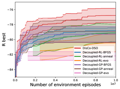
(a) Acrobot-v1

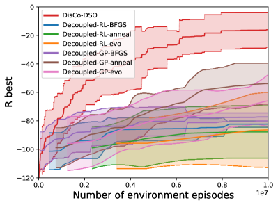
(b) LunarLander-v2

Figure 4: Reward of the best solution versus number of function evaluations on the decision tree policy task, for Acrobot-v1 and LunarLander-v2.

Evaluation.

For evaluation, we follow other works in the field (Silva et al., 2020; Ding et al., 2020; Custode and Iacca, 2023) and use the OpenAI Gym’s (Brockman et al., 2016) environments MountainCar-v0, CartPole-v1, Acrobot-v1, and LunarLander-v2. We investigate the sample-efficiency of DisCo-DSO on the decision tree policy task when compared to the decoupled baselines described at the beginning of this section. We train each algorithm for 10 different random seeds.

Results.

In Figure 4 (see also Figure 8 in the appendix), we report the mean and standard deviation of the best reward found by each algorithm versus number of environment episodes. These results show that DisCo-DSO dominates the baselines in terms of sample-efficiency. The trend is consistent across all environments, and is more pronounced in the more complex environments. The efficient use of evaluations by DisCo-DSO (each sample is a complete well-defined decision tree) versus the decoupled approaches, where each sample is a discrete skeleton that requires many evaluations to get a single complete solution, becomes a significant advantage in the RL environments where each evaluation involves running the environment for $N$ episodes.

Literature comparisons.

We conduct a performance comparison of DisCo-DSO against various baselines in the literature, namely evolutionary decision trees as detailed in Custode and Iacca (2023), cascading decision trees introduced in Ding et al. (2020), and interpretable differentiable decision trees (DDTs) introduced in Silva et al. (2020). In addition, we provide results with a BO baseline, where the structure of the decision tree is fixed to a binary tree of depth 4 without prefix-dependent positional constraints. Whenever a method provides a tree structure for a specific environment, we utilize the provided structure and assess it locally. In cases where the method’s implementation is missing, we address this by leveraging open-source code. This approach allows us to train a tree in absent environments, ensuring that we obtain a comprehensive set of results for all methods evaluated across all environments. The decision trees found by DisCo-DSO are shown in Figure 5 (see also Figure 9 in the appendix). Comparisons are shown in Table 1. Methods we trained locally are marked with an asterisk (*). Critically, we ensure consistent evaluation across baselines by assessing each decision tree policy on an identical set of 1,000 random seeds per environment.

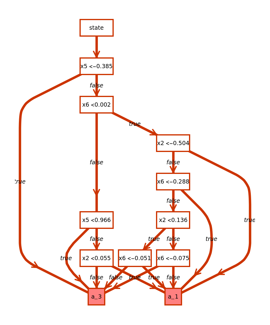
(a) Acrobot-v1

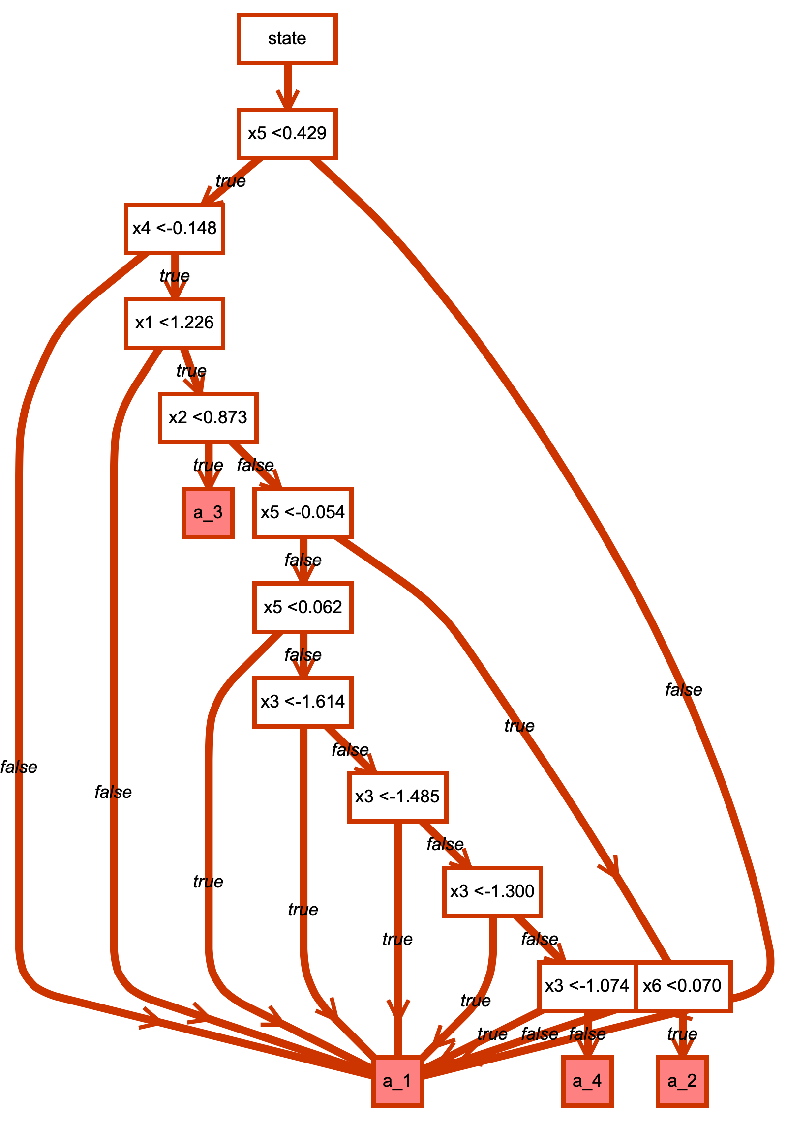
(b) LunarLander-v2

Figure 5: Best decision trees found by DisCo-DSO on the decision tree policy tasks for Acrobot-v1 and LunarLander-v2.

Algorithm	Acrobot-v1		CartPole-v1		LunarLander-v2		MountainCar-v0
	MR	PC	MR	PC	MR	PC	MR	PC
DisCo-DSO	-76.58	18	500.00	14	99.24	23	-100.97	15
Evolutionary DTs	-97.12*	5	499.58	5	-87.62*	17	-104.93	13
Cascading DTs	-82.14*	58	496.63	22	-227.02	29	-200.00	10
Interpretable DDTs	-497.86*	15	389.79	11	-120.38	19	-172.21*	15
Bayesian Optimization†	-90.99*	7	85.47*	7	-112.14*	7	-200.0*	7

Table 1: Evaluation of the best univariate decision trees found by DisCo-DSO and other baselines on the decision tree policy task. Here, MR is the mean reward earned in evaluation over a set of 1,000 random seeds, while PC represents the parameter count in each tree. For models trained in-house (*), the figures indicate the parameter count after the discretization process. ^†The topology of the tree is fixed for BO.

In Table 1 we also show the complexity of the discovered decision tree as measured by the number of parameters in the tree. We count every (internal or leaf) node of univariate decision trees (produced by all methods except for Cascading decision trees) as one parameter. For Cascading decision trees, the trees contain feature learning trees and decision making trees. The latter is just univariate decision trees, so the same complexity measurement is used. For the leaf nodes of feature learning trees, the number of parameters is number of observations times number of intermediate features. From Table 1, we observe that the univariate decision trees found by DisCo-DSO have the best performance on all environments at a comparable or lower complexity than the other literature baselines.

Symbolic regression for equation discovery

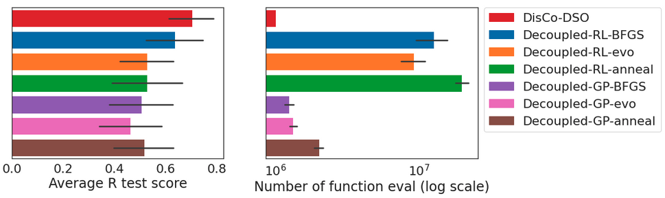
Figure 6: Average test set reward (left) and number of function evaluations (right) used across methods on the symbolic regression task. Recall that Decoupled-RL-BFGS and Decoupled-GP-BFGS correspond to the methods proposed in Petersen et al. (2021a) and Koza (1994), respectively. DisCo-DSO achieves the best average reward on the test set at the lowest number of function evaluations.

Problem formulation.

Symbolic regression (SR) (Koza, 1994; Bongard and Lipson, 2007; Petersen et al., 2021a; Landajuela et al., 2021a; de Franca et al., 2024) is a classical discrete-continuous optimization problem with applications in many fields, including robotics, control, and machine learning. In SR, we have $\mathcal{L}=\{x_{1},\ldots,x_{d},+,-,\times,\div,\sin,\cos,\ldots\}$ and $\hat{\mathcal{L}}=\{\text{const}(\beta)\}$, where $\text{const}(\beta)$ represents a constant with value $\beta$. The design space is a subset of the space of continuous functions, $\mathbb{T}\subset C(V^{\mathbb{R}})$, where $V\subset\mathbb{R}^{d}$ is the function support that depends on $\mathcal{L}$. The evaluation operator ${\tt eval}$ returns the function which expression tree has the sequence $\tau$ as pre-order traversal (depth-first and then left-to-right). For example, ${\tt eval}(\langle+,\cos,y,\times,\text{const}(3.14),\sin,x\rangle)=\cos(y)+3.14\times\sin(x)$. Given a dataset $D=\{(x_{1}^{(i)},\dots,x_{d}^{(i)},y^{(i)})\}_{i=1}^{N}$, the reward function is defined as the inverse of the normalized mean squared error (NMSE) between $y^{(i)}$ and ${\tt eval}(\tau)(x_{1}^{(i)},\dots,x_{d}^{(i)}),\forall i\in\{1,\dots,N\}$, computed as $\frac{1}{1+\text{NMSE}}$. SR has been shown to be NP-hard even for low-dimensional data (Virgolin and Pissis, 2022). Prefix-dependent positional constraints are given in the appendix.

Evaluation.

A key evaluation metric for symbolic regression is the parsimony of the discovered equations, i.e., the balance between the complexity of the identified equations and their ability to fit the data. A natural way to measure it is to consider the generalization performance over a test set. A SR method could find symbolic expressions that overfit the training data (using for instance overly complex expressions), but those expressions will not generalize well to unseen data. For evaluating the generalization performance of various baselines, we rely on the benchmark datasets detailed in Table 6 of the appendix.

Results.

Results in Figure 6 demonstrate the superior efficiency and generalization capability of DisCo-DSO in the SR setting. In particular, DisCo-DSO achieves the best average reward on the test set and the lowest number of function evaluations. Note that for DisCo-DSO we have perfect control over the number of function evaluations as it is determined by the number of samples ($10^{6}$ in this case). The Decoupled-GP methods exhibit a strong tendency to overfit to the training data and perform poorly on the test set. This phenomenon is known as the bloat problem in the SR literature (Silva and Costa, 2009). We observe that the joint optimization of DisCo-DSO avoids this problem and achieve the best generalization performance.

Literature comparisons.

In Table 2, we compare DisCo-DSO against state-of-the-art methods in the SR literature. In addition to the baselines (Petersen et al., 2021a; Koza, 1994) described above, we compare against the methods proposed in Biggio et al. (2021) and Kamienny et al. (2022). Since the method in Biggio et al. (2021) is only applicable to $\leq 3$ dimensions, we consider the subset of benchmarks with $\leq 3$ dimensions. We observe that DisCo-DSO dominates all baselines in terms of average reward on the full test set. For the subset of benchmarks with $\leq 3$ dimensions, DisCo-DSO achieves comparative performance to the specialized method in Biggio et al. (2021).

Algorithm	Dim $\leq 3$	Dim $\geq 1$
DisCo-DSO	0.6632 $\pm$ 0.3194	$\bm{0.7045}$ $\pm$ 0.3007
Decoupled-RL-BFGS⋆	0.6020 $\pm$ 0.4169	0.6400 $\pm$ 0.3684
Decoupled-RL-evo	0.0324 $\pm$ 0.1095	0.0969 $\pm$ 0.2223
Decoupled-RL-anneal	0.1173 $\pm$ 0.2745	0.1436 $\pm$ 0.3015
Decoupled-GP-BFGS⋆⋆	0.5372 $\pm$ 0.4386	0.4953 $\pm$ 0.4344
Decoupled-GP-evo	0.0988 $\pm$ 0.1975	0.0747 $\pm$ 0.1763
Decoupled-GP-anneal	0.1615 $\pm$ 0.2765	0.1364 $\pm$ 0.2608
Kamienny et al. (2022)	0.6068 $\pm$ 0.1650	0.5699 $\pm$ 0.1065
Biggio et al. (2021)	$\bm{0.6858}$ $\pm$ 0.1995	N/A

Table 2: Comparison of DisCo-DSO against decoupled baselines and the methods proposed in Biggio et al. (2021) and Kamienny et al. (2022) on the symbolic regression task. Values are mean $\pm$ standard deviation of the reward across benchmarks (provided in Table 6 of the appendix). We group benchmarks because Biggio et al. (2021) is only applicable to $\leq 3$ dimensions. ^⋆ Petersen et al. (2021a). ^⋆⋆ Koza (1994).

Conclusion

We proposed DisCo-DSO (Discrete-Continuous Deep Symbolic Optimization), a novel approach to optimization in hybrid discrete-continuous spaces. DisCo-DSO uses a generative model to learn a joint distribution on discrete and continuous design variables to sample new hybrid designs. In contrast to standard decoupled approaches, in which the discrete skeleton is sampled first, and then the continuous variables are optimized separately, our joint optimization approach samples both discrete and continuous variables simultaneously. This leads to more efficient use of objective function evaluations, as the discrete and continuous dimensions of the design space can “communicate” with each other and guide the search. We have demonstrated the benefits of DisCo-DSO in challenging problems in symbolic regression and decision tree optimization, where, in particular, DisCo-DSO outperforms the state-of-the-art on univariate decision tree policy optimization for RL.

Regarding the limitations of DisCo-DSO, it is important to note that the method relies on domain-specific information to define the ranges of continuous variables. In cases where this information is not available and estimates are necessary, the performance of DisCo-DSO could be impacted. Furthermore, in our RL experiments, we constrain the search space to univariate decision trees. Exploring more complex search spaces, such as multivariate or “oblique” decision trees, remains an avenue for future research.

Appendix A Pseudocode for DisCo-DSO

In this section we present pseudocode for the DisCo-DSO algorithm. The algorithm is presented in Algorithm 1. We also provide pseudocode for the discrete-continuous sampling procedure in Algorithm 2. Algorithm 2 is called multiple times to form a batch in Algorithm 1. Note that for decision tree policies for reinforcement learning, the distribution, $\mathcal{D}$, used for sampling the next continuous token in Algorithm 2 is only truncated with bounds produced with Algorithm 3 at a decision tree node. Otherwise, the distribution is unbounded.

Algorithm 1 Discrete-Continuous Deep Symbolic Optimization

0: batch size $N$, reward function $R$, risk factor $\epsilon$, policy gradient function $S$, entropy coefficient $\lambda_{\mathcal{H}}$, learning rate $\alpha$

0: Best fitting design $\tau^{\star}=\langle(l_{1},\beta_{1}),\ldots,(l_{T},\beta_{T})\rangle^{\star}$

1: Initialize AR with parameters $\theta$, defining distribution over designs $p(\cdot|\theta)$

2: repeat

3:  $\mathcal{T}\leftarrow\{\tau^{(i)}=(l,\beta)_{1:{T_{i}}}^{(i)}\sim p(\cdot|\theta)\}_{i=1}^{N}$ Sample batch of $N$ discrete-continous designs (Algorithm 2)

4:  $\mathcal{R}\leftarrow\{R(\tau^{(i)})\}_{i=1}^{N}$ Compute rewards

5:  $R_{\epsilon}\leftarrow(1-{\epsilon})$-quantile of $\mathcal{R}$ Compute reward threshold

6:  $\mathcal{T}\leftarrow\{\tau^{(i)}:R(\tau^{(i)})\geq R_{\epsilon}\}$ Select subset of expressions above threshold

7:  $\mathcal{R}\leftarrow\{R(\tau^{(i)}):R(\tau^{(i)})\geq R_{\epsilon}\}$ Select corresponding subset of rewards

8:  $\hat{g_{1}}\leftarrow\textrm{ReduceMean}((\mathcal{R}-R_{\epsilon})S(\mathcal{T},\theta))$ Compute risk-seeking policy gradient

9:  $\hat{g_{2}}\leftarrow\textrm{ReduceMean}(-\lambda_{\mathcal{H}}\nabla_{\theta}\mathcal{H}(\mathcal{T}|\theta))$ Compute entropy gradient

10:  $\theta\leftarrow\theta+\alpha(\hat{g_{1}}+\hat{g_{2}})$ Apply gradients

11:  if $\max\mathcal{R}>R(\tau^{\star})$ then $\tau^{\star}\leftarrow\tau^{(\arg\max\mathcal{R})}$ Update best discrete-continuous design

12: return $\tau^{\star}$

Algorithm 2 Discrete-continuous sampling

0: parameters of the given AR $\theta$, token library $\mathcal{L}$

0: sequence $\tau=\langle(l_{1},\beta_{1}),\ldots,(l_{T},\beta_{T})\rangle$ sampled from the AR

1: $\tau=\tau_{1:0}\leftarrow[\cdot]$ Initialize empty sequence

2: for $i=1,2,\ldots$ do

3:  $(\psi^{(i)},\phi^{(i)})\leftarrow\text{AR}(\tau_{1:(i-1)}=(l,\beta)_{1:(i-1)};\theta)$ Emit two outputs for each token

4:  Compute $\mathcal{C}_{\tau_{1:(i-1)}}\subseteq\mathcal{L}$ Compute unfeasible tokens

5:  $\psi^{(i)}_{\mathcal{C}_{\tau_{1:(i-1)}}}\leftarrow-\infty$ Set unfeasible tokens to $-\infty$

6:  $l_{i}\leftarrow$ Categorical($\psi^{(i)}$) Sample the next discrete token

7:  if $l_{i}\in\bar{\mathcal{L}}$ then

8:   $\beta_{i}\leftarrow\mathcal{U}_{[0,1]}(\cdot)$ Sample the next continuous token

9:  else if $l_{i}\in\hat{\mathcal{L}}$ then

10:   $\beta_{i}\leftarrow\mathcal{D}(\cdot|l_{i},\phi^{(i)})$ Sample the next continuous token

11:  end if

12:  $\tau_{i}\leftarrow(l_{i},\beta_{i})$ Joint discrete and continuous token

13:  $\tau\leftarrow\tau\mathbin{\|}\tau_{i}$ Append token to traversal

Appendix B Additional algorithm details

Risk-seeking policy gradient for hybrid discrete-continuous action space

The derivation of the risk-seeking policy gradient for the hybrid discrete-continuous action space follows closely the derivation in Petersen et al. [2021a] (see also Tamar et al. [2014]). The risk-seeking policy gradient for a univariate sequence $\tau$ is given by

$$\nabla_{\theta}J_{\varepsilon}(\theta) =\mathbb{E}_{\tau\sim p(\tau|\theta)}\left[\left(R(\tau)-R_{\varepsilon}(\theta)\right)\nabla_{\theta}\log p(\tau|\theta)\mid R(\tau)\geq R_{\varepsilon}(\theta)\right].$$

In the hybrid discrete-continuous action space case, we have $\tau=\langle(l_{1},\beta_{1}),\ldots,(l_{T},\beta_{T})\rangle$ and

$$p(\tau|\theta)=\prod_{i=1}^{|\tau|}p(\tau_{i}|\tau_{1:(i-1)},\theta)=\prod_{i=1}^{|\tau|}p((l_{i},\beta_{i})|(l,\beta)_{1:(i-1)},\theta).$$ (4)

Thus, using the convenient notation $A(\tau,\varepsilon,\theta)=R(\tau)-R_{\varepsilon}(\theta)$, the risk-seeking policy gradient for the hybrid discrete-continuous action space is given by

$$\nabla_{\theta}J_{\varepsilon}(\theta)=\mathbb{E}_{\tau\sim p(\tau|\theta)}\left[A(\tau,\varepsilon,\theta)\nabla_{\theta}\log p(\tau|\theta)\mid A(\tau,\varepsilon,\theta)\geq 0\right]$$

$$=\mathbb{E}_{\tau\sim p(\tau|\theta)}\left[A(\tau,\varepsilon,\theta)\nabla_{\theta}\log\prod_{i=1}^{|\tau|}p((l_{i},\beta_{i})|(l,\beta)_{1:(i-1)},\theta)\mid A(\tau,\varepsilon,\theta)\geq 0\right]$$

$$=\mathbb{E}_{\tau\sim p(\tau|\theta)}\left[A(\tau,\varepsilon,\theta)\sum_{i=1}^{|\tau|}\nabla_{\theta}\log p((l_{i},\beta_{i})|(l,\beta)_{1:(i-1)},\theta)\mid A(\tau,\varepsilon,\theta)\geq 0\right]$$

$$=\mathbb{E}_{\tau\sim p(\tau|\theta)}\left[A(\tau,\varepsilon,\theta)\sum_{i=1}^{|\tau|}\begin{cases}\nabla_{\theta}\log p(l_{i}|(l,\beta)_{1:(i-1)},\theta),&\text{if }l_{i}\in\bar{\mathcal{L}}\\ \nabla_{\theta}\log p(\beta_{i}|l_{i},(l,\beta)_{1:(i-1)},\theta)+\nabla_{\theta}\log p(l_{i}|(l,\beta)_{1:(i-1)},\theta),&\text{if }l_{i}\in\hat{\mathcal{L}}\end{cases}\mid A(\tau,\varepsilon,\theta)\geq 0\right].$$

In practice, we use the following estimator for the risk-seeking policy gradient:

$$\nabla_{\theta}J_{\varepsilon}(\theta)\approx\frac{1}{M}\sum_{i=1}^{M}\tilde{A}(\tau^{(i)},\varepsilon,\theta)\sum_{j=1}^{|\tau^{(i)}|}\begin{cases}\nabla_{\theta}\log p(l_{j}^{(i)}|(l,\beta)_{1:(j-1)}^{(i)},\theta),&\text{if }l_{j}^{(i)}\in\bar{\mathcal{L}}\\ \nabla_{\theta}\log p(\beta_{j}^{(i)}|l_{j}^{(i)},(l,\beta)_{1:(j-1)}^{(i)},\theta)+\\ \quad\quad\nabla_{\theta}\log p(l_{j}^{(i)}|(l,\beta)_{1:(j-1)}^{(i)},\theta),&\text{if }l_{j}^{(i)}\in\hat{\mathcal{L}}\end{cases}$$

$$\ \ \ \ \ \ \ \ \ \ \ \ \ \ \ \ \ \ \ \ \ \ \ \ \ \ \ \ \ \ \ \ \ \ \ \ \ \ \ \ \ \ \ \ \ \ \ \ \ \ \ \ \ \ \ \ \ \ \ \ \ \ \ \ \ \ \ \ \ \ \cdot\mathbb{I}(\tilde{A}(\tau^{(i)},\varepsilon,\theta)\geq 0),$$

where $\tau^{(i)}=\langle(l_{1}^{(i)},\beta_{1}^{(i)}),\ldots,(l_{T}^{(i)},\beta_{T}^{(i)})\rangle$ is the $i$-th trajectory sampled from $p(\tau|\theta)$, $M$ is the number of trajectories used in the estimator, and $A(\tau^{(i)},\varepsilon,\theta)\approx\tilde{A}(\tau^{(i)},\varepsilon,\theta)=R(\tau^{(i)})-\tilde{R}_{\varepsilon}(\theta)$, with $\tilde{R}_{\varepsilon}(\theta)$ being an estimate of $R_{\varepsilon}(\theta)$.

Entropy derivation in the hybrid discrete-continuous action space

As in Petersen et al. [2021a], we add entropy to the loss function as a bonus. Since there is a continuous component in the library, the entropy for the distribution of $\tau_{i}$ in the sequence is

$$\mathcal{H}_{i}=\sum_{l\in\hat{\mathcal{L}}}p(l|(l,\beta)_{1:(i-1)},\theta)\mathcal{H}_{\beta\sim\mathcal{D}(\beta|l,\phi_{l})}(\beta|l)+\mathcal{H}_{l\sim p(l|(l,\beta)_{1:(i-1)},\theta)}(l).$$

For the derivation, recall that, for a distribution $\mathcal{D}$, the entropy is defined as $\mathcal{H}(\mathcal{D})=-\int_{-\infty}^{\infty}\mathcal{D}(x)\log\mathcal{D}(x)\,dx,$ and that, in DisCo-DSO, we add an entropy regularization term for each distribution $p((l_{i},\beta_{i})|(l,\beta)_{1:(i-1)},\theta)$ encountered during the rollout. Thus, we have

$$\begin{split}\mathcal{H}_{i}=&-\sum_{l_{i}\in\hat{\mathcal{L}}}\int_{-\infty}^{\infty}p((l_{i},\beta_{i})|(l,\beta)_{1:(i-1)},\theta)\log p((l_{i},\beta_{i})|(l,\beta)_{1:(i-1)},\theta)\,d\beta_{i}\\ &\hskip 113.81102pt-\sum_{l_{i}\in\bar{\mathcal{L}}}p(l_{i}|(l,\beta)_{1:(i-1)},\theta)\log p(l_{i}|(l,\beta)_{1:(i-1)},\theta)\\ =&-\sum_{l_{i}\in\hat{\mathcal{L}}}\int_{-\infty}^{\infty}p(\beta_{i}|l_{i})p(l)\log\left(p(\beta_{i}|l_{i})p(l_{i})\right)\,d\beta_{i}-\sum_{l_{i}\in\bar{\mathcal{L}}}p(l_{i})\log p(l_{i})\\ =&-\sum_{l_{i}\in\hat{\mathcal{L}}}\int_{-\infty}^{\infty}p(\beta_{i}|l_{i})p(l_{i})\log p(\beta_{i}|l_{i})\,d\beta_{i}-\sum_{l_{i}\in\hat{\mathcal{L}}}\int_{-\infty}^{\infty}p(\beta_{i}|l_{i})p(l_{i})\log p(l_{i})\,d\beta_{i}\\ &\ \ \ \ \ \ \ \ -\sum_{l_{i}\in\bar{\mathcal{L}}}p(l_{i})\log p(l_{i})\\ =&-\sum_{l_{i}\in\hat{\mathcal{L}}}p(l_{i})\int_{-\infty}^{\infty}p(\beta_{i}|l_{i})\log p(\beta_{i}|l_{i})\,d\beta_{i}-\sum_{l_{i}\in\hat{\mathcal{L}}}p(l_{i})\log p(l_{i})\int_{-\infty}^{\infty}p(\beta_{i}|l_{i})\,d\beta_{i}\\ &\ \ \ \ \ \ \ \ -\sum_{l_{i}\in\bar{\mathcal{L}}}p(l_{i})\log p(l_{i})\\ =&\sum_{l_{i}\in\hat{\mathcal{L}}}p(l_{i}|(l,\beta)_{1:(i-1)},\theta)\mathcal{H}_{\beta_{i}\sim\mathcal{D}(\beta_{i}|l_{i},\phi_{l_{i}})}(\beta_{i}|l_{i})\\ &\ \ \ \ \ \ \ \ -\sum_{l_{i}\in\mathcal{L}}p(l_{i}|(l,\beta)_{1:(i-1)},\theta)\log p(l_{i}|(l,\beta)_{1:(i-1)},\theta).\end{split}$$

Note that we have removed the conditioning elements $\theta$ and $(l,\beta)_{1:(i-1)}$ in some terms in the above derivation for brevity.

Appendix C Additional experimental results per task

Parameterized bitstring task

Objective functions.

The objective functions $f_{1}$ and $f_{2}$ in Equation 3 are plotted in Figure 7. They are both non-differentiable and difficult to be optimized by Quasi-Newton methods.

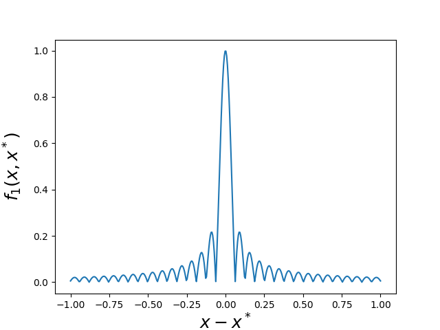
(a) $f_{1}$

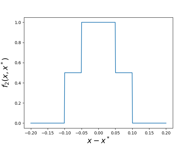
(b) $f_{2}$

Figure 7: Objective functions in equation 3 against the difference $x-x^{*}$.

Objective gap between the best solutions found by DisCo-DSO and baselines for the parameterized bitstring task.

In Table 3, we show the gap between the best solutions obtained by DisCo-DSO and the baselines for the parameterized bitstring task. The gap is computed by taking the best DisCo-DSO solutions and the best solutions of the baselines for each seed. The reward differences are averaged over the 5 seeds.

Baseline	$f_{1}$, $\alpha=0.5$	$f_{1}$, $\alpha=0.9$	$f_{2}$, $\alpha=0.5$	$f_{2}$, $\alpha=0.9$
Decoupled-RL-BFGS	0.1263	0.0123	0.1433	0.0253
Decoupled-RL-evo	0.0970	0.0100	0.0833	0.0187
Decoupled-RL-anneal	0.1211	0.0095	0.1000	0.0140

Table 3: Gap between the best solutions found by DisCo-DSO and baselines for the parameterized bitstring task. Positive values indicate that DisCo-DSO found better solutions.

Decision tree policies for reinforcement learning

Results for MountainCar-v0 and CartPole-v1 environments.

In this section, we provide results for the MountainCar-v0 and CartPole-v1 environments. In Figure 8, we show the best reward versus number of environment episodes for MountainCar-v0 and CartPole-v1. Figure 9 shows the best decision trees found by DisCo-DSO for MountainCar-v0 and CartPole-v1.

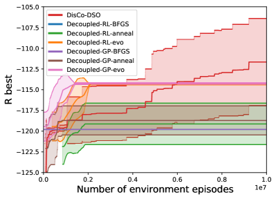
(a) MountainCar-v0

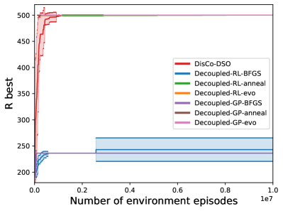
(b) CartPole-v1

Figure 8: Reward of the best solution versus number of function evaluations on the decision tree policy task, for MountainCar-v0 and CartPole-v1.

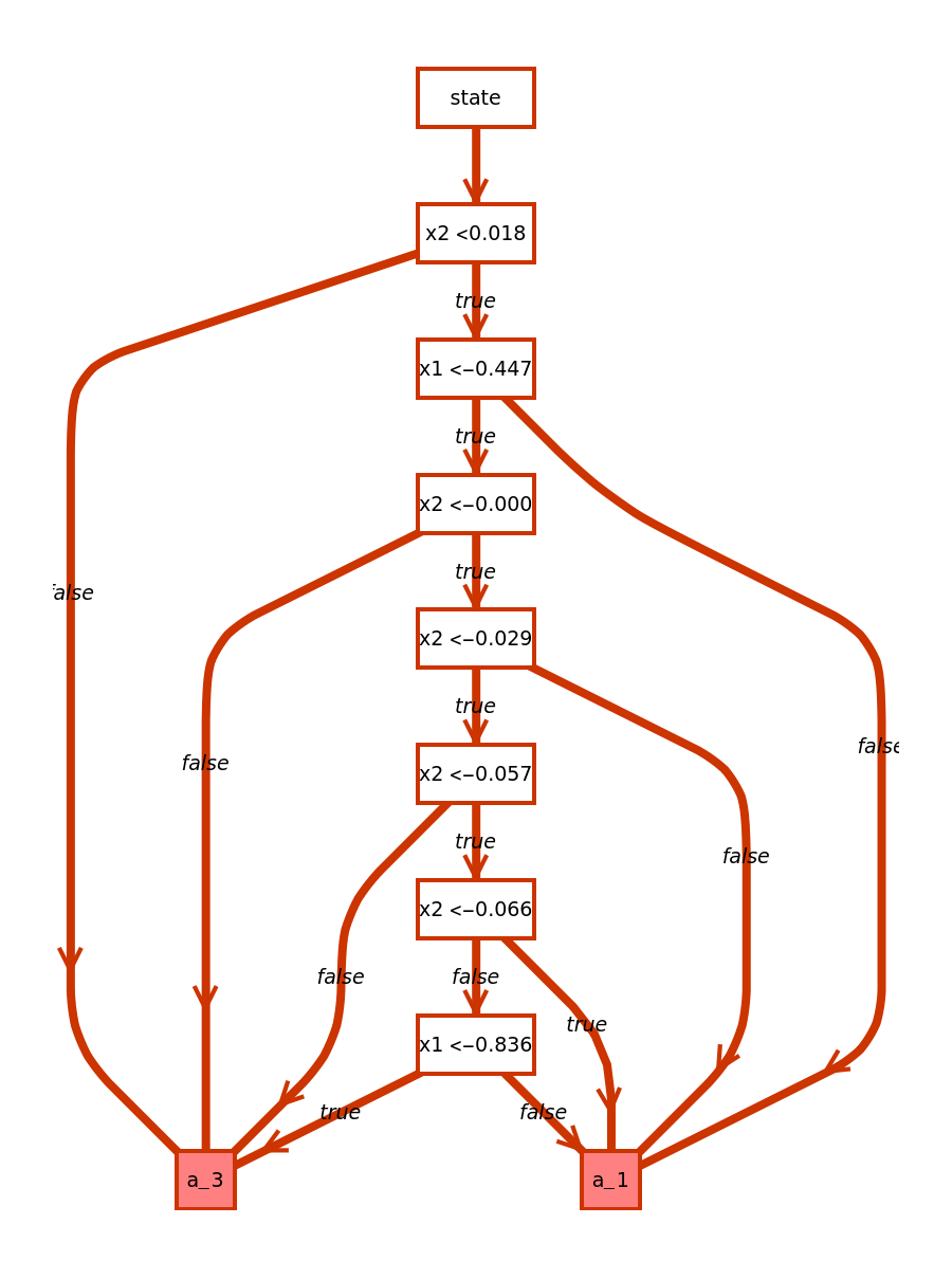
(a) MountainCar-v0

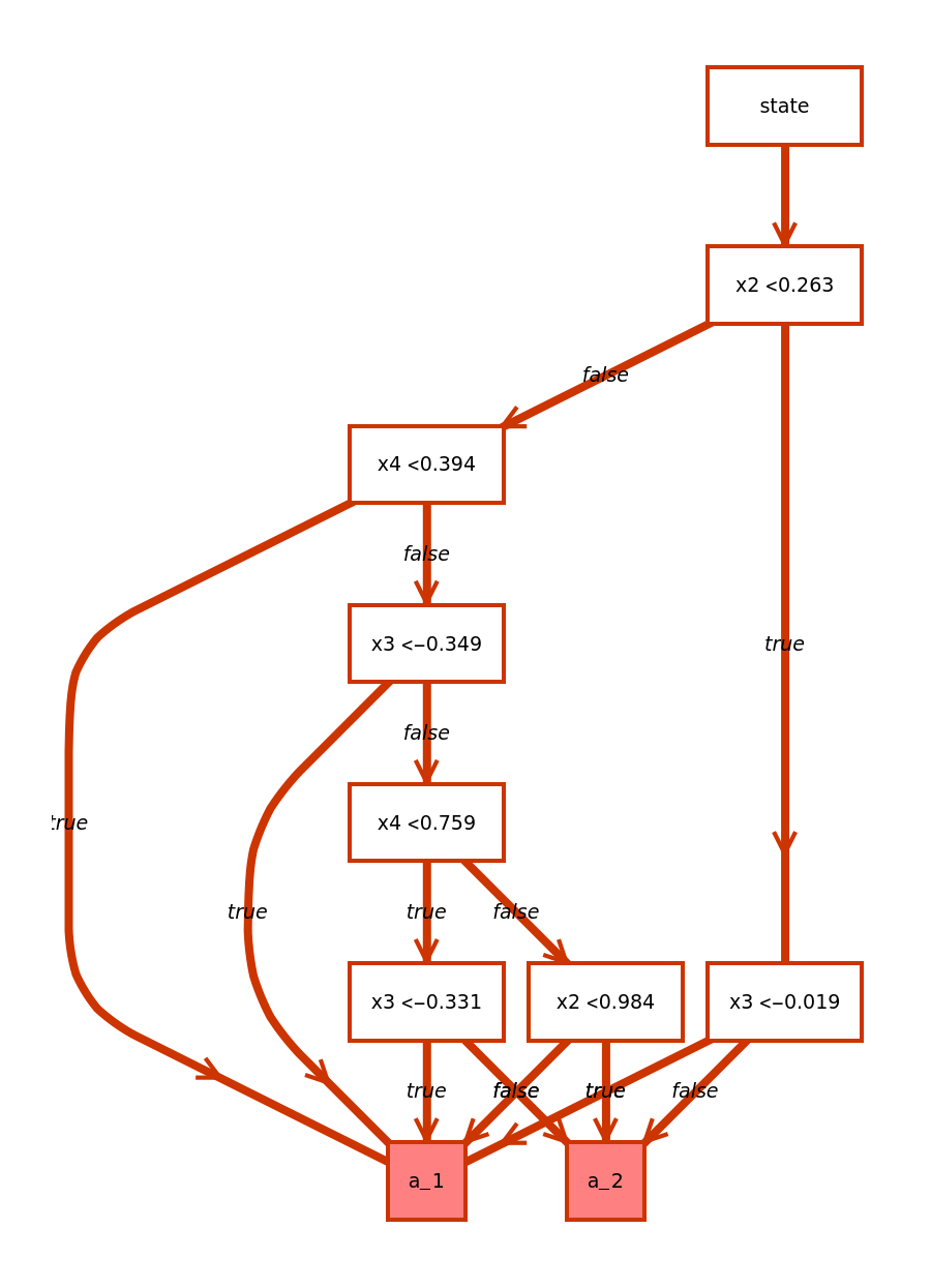
(b) CartPole-v1

Figure 9: Best decision trees found by DisCo-DSO on the decision tree policy tasks for MountainCar-v0 and CartPole-v1.

Note on “oblique” decision trees.

Custode and Iacca [2023] consider multivariate, or ”oblique” decision trees. These are trees where the left-hand side of a decision node is composed of an expression, while the right-hand side is still a boolean decision parameter $\beta_{n}$. While these trees perform well on more complex environments such as LunarLander-v2 (published results report an average test score of 213.09), we do not compare against them here as the search space is drastically different.

Objective gap between the best solutions found by DisCo-DSO and baselines for the decision tree policy task.

In Table 4 and Table 5, we show the objective gap between the best solutions found by DisCo-DSO and the baselines for the decision tree policy task. The gap is computed by taking the best DisCo-DSO solutions and the best solutions of the baselines.

Baseline	CartPole-v1	MountainCar-v0	LunarLander-v2	Acrobot-v1
Decoupled-RL-BFGS	260.00	7.80	74.80	4.22
Decoupled-RL-evo	0.00	2.60	80.60	6.52
Decoupled-RL-anneal	0.00	7.10	79.60	4.52
Decoupled-GP-BFGS	265.00	7.70	64.80	4.72
Decoupled-GP-evo	0.00	2.80	54.60	7.92
Decoupled-GP-anneal	0.00	6.10	43.20	4.52

Table 4: Objective gap between the best solutions found by DisCo-DSO and baselines for the decision tree policy task. Positive values indicate that DisCo-DSO found better solutions.

Baseline	CartPole-v1	MountainCar-v0	LunarLander-v2	Acrobot-v1
Evolutionary DTs	0.42	3.96	186.86	20.54
Cascading DTs	3.37	99.03	326.26	5.56
Interpretable DDTs	110.21	71.24	219.62	421.28
Bayesian Optimization	414.53	99.03	211.38	14.41

Table 5: Objective gap between the best solutions found by DisCo-DSO and baselines from the literature for the decision tree policy task. Positive values indicate that DisCo-DSO found better solutions.

Symbolic regression for equation discovery with constants

Additional details on the evaluation procedure for symbolic regression.

For evaluating the generalization performance of various baselines, we rely on the benchmark datasets detailed in Table 6. The test set is obtained by expanding the benchmark’s domain $(a,b)$ and increasing the number of data points on which an expression is evaluated. Since all experiments were conducted with 10 different random seeds, each random seed leads to a distinct “best” expression for that specific run. We take each of these 10 best expressions and compute the reward obtained on the evaluation dataset. Additionally, we calculate the number of function evaluations required to arrive at each expression. Subsequently, we aggregate the set of 10 evaluation rewards to calculate a single average reward and a single average number of function evaluations for each dataset. Following this procedure, we average over all the datasets to get an overall evaluation for each method.

Benchmarks.

In Table 6, we provide a compilation of benchmarks used in the symbolic regression task. The list comprises Livermore benchmarks from Mundhenk et al. [2021], Jin benchmarks from Jin et al. [2020], and Neat and Korn benchmarks from Trujillo et al. [2016]. We also introduce Constant benchmarks, which are a variation of the Nguyen benchmarks from Uy et al. [2011] where floating constants are added to increase the complexity of the problem. Note that the selection of these benchmarks is not arbitrary. The linear and non-linear dependency of the expressions on $\beta_{i}$ is taken into consideration. Non-linear functions involving $\beta_{i}$ exhibit more complicated expressions, thus rendering more challenges for the optimization problem. On the other hand, linear functions, such as Jin-1, employ constants as coefficients for each variable term, thereby simplifying the optimization problems into linear regression problems. Consequently, we have selected approximately 25 non-linear functions and 20 linear functions, resulting in a total of 45 benchmark datasets. Exploring whether joint discrete-continuous optimization can outperform other classes of methods for both non-linear functions and linear functions can be a focus for future research.

Evaluations sets.

To create the evaluation set, we adhere to a straightforward rule: we take the training set of each benchmark function, double the size of its domain, and double the number of points at which it is computed. For instance, a benchmark function with a training domain of $(-1,1)$ and 20 points in that domain would have an evaluation set spanning $(-2,2)$ with 40 data points within the expanded domain.

Benchmark Name	Expression	Dataset
Livermore2-Vars2-2	$x_{1}\,x_{2}\,\left(x_{1}+x_{1}\,\sqrt{x_{2}\,(\beta_{1}+x_{1}+\beta_{2}\,x_{1}\,x_{2}+\beta_{3}\,x_{2}^{3})}\right)$	U(-10,10,1000)
Livermore2-Vars2-4	$\beta_{1}\,x_{1}+\beta_{2}\,x_{2}+(x_{1}-x_{2})^{2}$	U(-10,10,1000)
Livermore2-Vars2-6	$-\left((x_{1}-x_{1}^{2}-x_{2})\,x_{2}\right)+\frac{(\beta_{1}\,x_{1})}{(\beta_{2}+\beta_{3}\,x_{2})}$	U(-10,10,1000)
Livermore2-Vars2-7	$1+\beta_{1}\,\sqrt{x_{1}}+\beta_{2}\,x_{1}+\frac{(\beta_{3}\,x_{2})}{x_{1}}+\beta_{4}\,\sqrt{-x_{1}+x_{2}}$	U(-10,10,1000)
Livermore2-Vars2-8	$\beta_{1}\,x_{1}^{2}+\beta_{2}\,x_{2}^{2}+\beta_{3}\,x_{2}^{3}+\frac{((\sqrt{x_{1}}-x_{1})\,\log{(x_{2})})}{\log{(x_{1})}}$	U(-10,10,1000)
Livermore2-Vars2-12	$\sqrt{(x_{1}+\frac{x_{2}}{e^{x_{2}}})\,\log(\beta_{1}\,x_{1}^{3}+\beta_{2}\,x_{1}^{2}\,x_{2}+\beta_{3}\,x_{2}^{3})}$	U(-10,10,1000)
Livermore2-Vars2-24	$\beta_{1}+\beta_{2}\,x_{1}+\beta_{3}\,(x_{1}-x_{2}^{2})^{2}$	U(-10,10,1000)
Livermore2-Vars3-4	$\beta_{1}+\beta_{2}x_{2}x_{3}+x_{1}+x_{2}+\sqrt{\cos(x_{2}})+x_{3}$	U(-10,10,1000)
Livermore2-Vars2-9	$\beta_{1}+x_{1}+x_{1}^{2}-x_{2}+\beta_{2}\,\sqrt{1+\beta_{3}\,x_{1}+\beta_{4}\,x_{2}}$	U(-10,10,1000)
Livermore2-Vars2-16	$-\left((x_{1}-x_{1}^{2}-x_{2})\,x_{2}\right)+\frac{(\beta_{1}\,x_{1})}{(\beta_{2}+\beta_{3}\,x_{2})}$	U(-10,10,1000)
Livermore2-Vars2-17	$x_{1}-\sqrt{x_{1}}\,x_{2}-\sin{\left(\log{(\beta_{1}\,x_{1}+\beta_{2}\,x_{1}^{3}+\beta_{3}\,x_{2}^{2})}\right)}^{2}$	U(-10,10,1000)
Livermore2-Vars2-19	$\left(x_{1}+\frac{(\beta_{1}*\cos{(x1)})}{\sqrt{1+\beta_{2}\,x_{1}+\beta_{3}\,x_{1}\,(x_{2}^{2}+\log{(x_{2})})}}\right)\,(x_{1}+\sin{(1)})$	U(-10,10,1000)
Livermore2-Vars2-22	$\frac{\log{(\beta_{1}\,(-1+\beta_{2}\,x_{1})^{2}+\frac{(e^{x_{2}}\,x_{1})}{\sqrt{\cos{(\beta_{3}*x_{2})}}})}}{\sqrt{x_{1}}}$	U(-10,10,1000)
Livermore2-Vars2-23	$x_{1}^{2}+\beta_{1}\,\sqrt{1+\frac{(\beta_{2}\,(\beta_{3}-x_{2})\,(\beta_{4}+\log{x_{2}}))}{x_{1}}}$	U(-10,10,1000)
Livermore2-Vars3-2	$\frac{(\beta_{1}\,(\beta_{2}\,x_{1}-x_{2})^{2}\,(\beta_{4}-x_{3})^{2})}{(1+\beta_{3}\,x_{2}^{2})^{2}}$	U(-10,10,1000)
Livermore2-Vars3-8	$\frac{x_{1}}{\left((e^{(x_{2}+x_{2}^{4})}+\beta_{1}\,x_{1}^{2}+\beta_{2}\,x_{1}^{2}\,x_{3}+\beta_{3}\,x_{3}^{2})\,(-x_{2}+x_{3}+\sqrt{\frac{\log{(x_{3})}}{(x_{1}^{2}+\sqrt{x_{3}})}})\right)}$	U(-10,10,1000)
Livermore2-Vars3-9	$x_{1}\,\sin{\left(\frac{(\beta_{1}\,x_{1})}{\sqrt{\beta_{2}\,x_{1}^{2}-\frac{(x_{1}\,(-1+x_{1}+x_{2}^{2})^{4}\,\sqrt{x_{2}+\beta_{3}\,x_{1}\,x_{3}^{2}})}{x_{3}}}}\right)}$	U(-10,10,1000)
Livermore2-Vars3-11	$\beta_{1}\,x_{1}+\frac{x_{1}}{x_{2}}+\beta_{2}\,x_{2}+\beta_{3}\,x_{3}$	U(-10,10,1000)
Livermore2-Vars3-12	$\beta_{1}+\beta_{2}\,x_{1}x_{2}^{2}+x_{2}+x_{3}$
Livermore2-Vars3-17	$\beta_{1}\,x_{1}+\beta_{2}\,x_{2}+x_{1}\sqrt{x_{2}}\cos(x_{1})+x_{3}+1$	U(-10,10,1000)
Livermore2-Vars3-20	$\beta_{1}+\beta_{2}\sqrt{\frac{\sqrt{x_{2}}}{\sqrt{x_{3}}}}+x_{1}$	U(-10,10,1000)
Livermore2-Vars3-24	$\beta_{1}+\beta_{2}\,x_{1}\,x_{2}^{2}+x_{2}+x_{3}$	U(-10,10,1000)
Livermore2-Vars4-8	$-x_{1}+x_{1}\,\left(x_{1}+x_{4}+\sin{\left(\frac{(-(e^{e^{x_{3}}}\,x_{1})+x_{2})}{(\beta_{1}\,x_{1}^{2}\,x_{3}+\beta_{2}\,x_{3}^{2}+\beta_{3}\,x_{3}^{3})}\right)}\right)$	U(-10,10,1000)
Livermore2-Vars4-16	$x_{3}\left(\frac{\beta_{1}}{x_{3}}-x_{4}\right)+\frac{\beta_{2}\,x_{4}}{x_{1}}+\sqrt{x_{2}\left(x_{1}^{2}\left(-e^{x_{2}}\right)-x_{2}\right)}$	U(-10,10,1000)
Livermore2-Vars4-18	$x_{1}+\sin{\left(2\,x_{2}+x_{3}+\beta_{1}\,\sqrt{\beta_{2}+\beta_{3}\,x_{2}^{3}+x_{2}\,x_{3}^{2}}-e^{x_{1}}\,x_{4}+\log{((-x_{1}+x_{2})\,\log{(x_{2})})}\right)}$	U(-10,10,1000)
Livermore2-Vars4-23	$-(\frac{x_{1}}{x_{2}})+x_{2}+\beta_{1}\,x_{2}\,x_{3}+\frac{(\beta_{2}\,x_{3})}{\sqrt{x_{4}}}+\beta_{3}\,\sqrt{x_{4}}+\log{(x_{1})}$	U(-10,10,1000)
Livermore2-Vars6-22	$x_{1}+\cos{(x_{2}+\beta_{1}\,x_{5})}\,(x_{4}-\cos{(x_{6})}\,\sin{\left(\beta_{2}\,(\beta_{3}+x_{3}-x_{4})\right)})$	U(-10,10,1000)
Livermore2-Vars6-23	$x_{1}+x_{4}+\log{\left(x_{1}^{2}+x_{1}\left(\beta_{1}\,\sqrt{\beta_{2}\,x_{1}+x_{2}+\beta_{3}\,(x_{3}-\frac{x_{4}}{x_{5}})}-x_{6}\right)\right)}$	U(-10,10,1000)
Livermore2-Vars6-24	$\frac{\left(\beta_{1}\,\left(\beta_{2}\left(\beta_{3}\,x_{2}+\frac{\sqrt{x_{3}}}{(\sqrt{-x_{4}+x_{5}}\,x_{6})}\right)^{1/4}+\sin{(x_{1})}\right)\right)}{x_{6}}$	U(-10,10,1000)
Livermore2-Vars7-14	$\beta_{1}x_{6}+\beta_{2}\,x_{1}^{2}x_{6}-\cos\left(x_{7}\left(\frac{x_{2}^{2}x_{5}^{2}x_{6}^{2}(x_{1}+x_{3}\,x_{4}\,x_{6})^{2}+x_{6}}{x_{1}}+x_{7}\right)\right)$	U(-10,10,1000)
Livermore2-Vars7-23	$-\left(\frac{(\sqrt{x_{3}}x_{4})}{(x_{3}+x_{5}+\beta_{1}\,x_{2}\,x_{3}\,x_{5}+\beta_{2}\,x_{2}\,x_{6}+\beta_{3}\,x_{4}\,x_{6}\,x_{7}+(-x_{6}+x_{7})^{2})}\right)+x_{1}\,\cos{(x_{1})}+\cos{(x_{2})}$	U(-10,10,1000)
Jin-1	$\beta_{1}\,x_{1}^{3}+\beta_{2}\,x_{1}^{4}+\beta_{3}\,x_{2}+\beta_{4}\,x_{2}^{2}$	U(-3,3,100)
Jin-2	$\beta_{1}+\beta_{2}\,x_{1}^{2}+\beta_{3}\,x_{2}^{3}$	U(-3,3,100)
Jin-3	$\beta_{1}\,x_{1}+\beta_{2}\,x_{1}^{3}+\beta_{3}\,x_{2}+\beta_{4}\,x_{2}^{3}$	U(-3,3,100)
Jin-6	$\beta_{1}\,x_{1}\,x_{2}+\beta_{2}\sin((\beta_{3}+x_{1})(\beta_{4}+x_{2}))$	U(-3,3,100)
Korn-12	$2+\beta_{1}\cos(\beta_{2}\,x_{1})\sin(\beta_{3}\,x_{5})$	U(-50,50,100)
Neat-7	$2+\beta_{1}\cos(\beta_{2}\,x_{1})\sin(\beta_{3}\,x_{2})$	U(-50,50,10000)
Constant-1	$\beta_{1}\,x_{1}+\beta_{2}\,x_{1}^{2}+\beta_{3}\,x_{1}^{3}$	U(-1,1,20)
Constant-2	$\beta_{1}+\sin\left(x_{1}^{2}\right)\cos(x_{1})$	U(-1,1,20)
Constant-3	$\cos(x_{1}\,x_{2})\sin(\beta_{2}\,x_{1})$	U(0,1,20)
Constant-4	$\beta_{1}\,x_{1}^{x_{2}}$	U(0,1,20)
Constant-5	$\beta_{1}\,\sqrt{x_{1}}$	U(0,4,20)
Constant-6	$x_{1}^{\beta_{1}}$	U(0,4,20)
Constant-7	$2\cos(x_{2})\sin(\beta_{1}\,x_{1})$	U(0,1,20)
Constant-8	$\log(\beta_{1}+x_{1})+\log\left(\beta_{2}+x_{1}^{2}\right)$	U(0,4,20)

Table 6: List of benchmarks used for symbolic regression task. Each benchmark includes input variables denoted as $x_{1},x_{2},\ldots,x_{d}$, along with floating constants denoted as $\beta_{i}$. The notation U$(a,b,c)$ denotes the inclusion of $c$ random points uniformly sampled from the open interval $(a,b)$ for each input variable $x_{i}$.

Analysis of traversal lengths generated in symbolic regression task.

Figure 10 shows the distribution of traversal lengths sampled by each method. These traversals are gathered from the top-performing expressions sampled, in the same way as the traversals used to generate Figure 6. Notice the extreme density placed at the maximum length (32) by the Decoupled-GP methods. This, paired with its poor generalization capability demonstrated in Figure 6a, leads us to conclude that the Decoupled-GP methods overfit heavily on the training data. The Decoupled-RL methods do this to a lesser degree, as does DisCo-DSO.

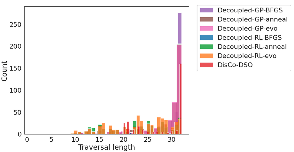
Figure 10: Histogram illustrating the lengths of traversals selected by different methods on the SR task.

Analysis of the effect of architecture and size of the autoregressive model in the symbolic regression task.

In Table 7, we provide a compilation of results obtained by using different autoregressive models of various sizes. Specifically, we consider a GRU and a LSTM recurrent cell with 16, 32 and 64 hidden units. We observe that the performance of the model is not very sensitive to the size of the model, although LSTM models tend to perform slightly better than GRU models. In this work, we use a LSTM model with 32 hidden units for all experiments.

Architecture	Mean R	Std R
DisCo-DSO-GRU16	0.7377	0.3161
DisCo-DSO-GRU32	0.7092	0.3442
DisCo-DSO-GRU64	0.7236	0.3261
DisCo-DSO-LSTM16	0.7385	0.3177
DisCo-DSO-LSTM32	0.7391	0.3134
DisCo-DSO-LSTM64	0.7302	0.3182

Table 7: Experiments with symbolic regression repeated using different autoregressive models of various sizes. Specifically, we consider a GRU and a LSTM recurrent cell with 16, 32 and 64 hidden units.

Objective gap between the best solutions found by DisCo-DSO and baselines for symbolic regression for equation discovery task.

In Table 8 and Table 9, we show the objective gap between the best solutions found by DisCo-DSO and the baselines for the symbolic regression task. The gap is computed by taking the best DisCo-DSO solutions and the best solutions of the baselines.

Baseline	Dim $\leq$ 3	All Table 3
Decoupled-RL-BFGS	0.0612	0.0645
Decoupled-RL-evo	0.6308	0.6085
Decoupled-RL-anneal	0.5459	0.5609
Decoupled-GP-BFGS	0.126	0.2092
Decoupled-GP-evo	0.5644	0.6298
Decoupled-GP-anneal	0.5017	0.5681

Table 8: Objective gap between the best solutions found by DisCo-DSO and the baselines for the symbolic regression task. Positive values indicate that DisCo-DSO found better solutions.

Literature	Dim $\leq$ 3	All Table 3
Kamienny et al. (2022)	0.0564	0.1346
Biggio et al. (2021)	-0.0226	N/A

Table 9: Objective gap between the best solutions found by DisCo-DSO and the baselines for the symbolic regression task. Positive values indicate that DisCo-DSO found better solutions.

Appendix D Hyperparameters

In Table 10, we provide the common hyperparameters used for the RL-based generative methods (DisCo-DSO and Decoupled-RL). The hyperparameters for the GP-based method are provided in Table 11. DisCo-DSO’s specific hyperparameters, linked to modeling of the distribution $\mathcal{D}$, are provided in Table 12. For the DT policies for reinforcement learning task, the parameter $N$ (number of episodes to average over to compute a single reward $R(\tau)$) is set to 100.

Parameter	Value
Optimizer	Adam [Kingma and Ba, 2017]
Number of layers	1
Number of hidden units	32
RNN type	LSTM [Hochreiter and Schmidhuber, 1997]
Learning rate ($\alpha$)	0.001
Entropy coefficient ($\lambda_{\mathcal{H}}$)	0.01
Moving average coefficient $(\beta)$	0.5
Risk factor $(\epsilon)$	0.2

Table 10: DisCo-DSO and Decoupled-RL hyperparameters

Parameter	Value
Population size	1,000
Generations	1,000
Fitness function	NRMSE
Initialization method	Full
Selection type	Tournament
Tournament size $(k)$	5
Crossover probability	0.5
Mutation probability	0.5
Minimum subtree depth $(d_{\textrm{min}})$	0
Maximum subtree depth $(d_{\textrm{max}})$	2

Table 11: Decoupled-GP hyperparameters

Parameter	Value
Parameter shift	0.0
Parameter generating distribution scale $(\sigma)$	0.5
Learn parameter generating distribution scale	False
Parameter generating distribution type	Normal

Table 12: DisCo-DSO specific hyperparameters

Appendix E Performance Analysis

Our numerical experiments were conducted using 24 cores in parallel of an Intel Xeon E5-2695 v2 machine with 128 GB per node. The experiments were implemented in Python using TensorFlow.

For Decision Tree Policies for Reinforcement Learning, every single objective function evaluation requires running $N=100$ episodes of a reinforcement learning environment. In addition, the environment is reset after every episode, and the policy is evaluated on a new environment seed. This means that every single objective function evaluation requires running $N=100$ episodes on a new environment seed. Each episode requires running a decision tree policy on a full dynamical simulation of the environment. This task is computationally expensive, and the time per function evaluation is shown in Table 13.

Task	Time per function evaluation
CartPole-v1	0.89 s
MountainCar-v0	1.12 s
LunarLander-v2	1.66 s
Acrobot-v1	5.41 s

Table 13: Time per function evaluation for the Decision Tree Policies for Reinforcement Learning task.

To quantify improvements in terms of computational time of DisCo-DSO over the decoupled baselines, we provide in Table 14 the average computational efficiency for all the environments in the Decision Tree Policies for Reinforcement Learning task. We define computational efficiency as the ratio between the final objective value and the total time required to reach that value. We compare DisCo-DSO with the decoupled baselines.

Algorithm	CartPole-v1	MountainCar-v0	LunarLander-v2	Acrobot-v1
DisCo-DSO	485.94	-85.87	-8.07	-11.91
Decoupled-RL-BFGS	233.25	-91.88	-47.03	-12.58
Decoupled-RL-anneal	485.94	-91.34	-49.53	-12.63
Decoupled-RL-evo	485.94	-87.87	-50.05	-12.95
Decoupled-GP-BFGS	228.39	-91.80	-41.82	-12.66
Decoupled-GP-anneal	485.94	-90.57	-30.57	-12.63
Decoupled-GP-evo	485.94	-88.03	-36.51	-13.17

Table 14: Computational efficiency for the Decision Tree Policies for Reinforcement Learning task.

We can see that, as the scale of the problem increase (see Table 13), DisCo-DSO shows a significant improvement in terms of computational time compared to the decoupled baselines.

Appendix F Prefix-dependent positional constraints

The autoregressive sampling used by DisCo-DSO allows for the incorporation of task-dependent constraints. These constraints are applied in situ, i.e., during the sampling process. These ideas have been used by several works using similar autoregressive sampling procedures [Popova et al., 2019, Petersen et al., 2021a, b, Landajuela et al., 2021a, Mundhenk et al., 2021, Kim et al., 2021]. In this work, we include three novel constraints that are specific to the decision tree generation task, one on the continuous parameters and two on the discrete tokens.

Constraints for decision tree generation

Constraint on parameter range.

By using a truncated normal distribution, upper/lower bounds are imposed on the parameters of decision trees (i.e., $\beta_{n}$ in the Boolean expression tokens $x_{n}<\beta_{n}$) to prevent meaningless internal nodes from being sampled. In Algorithm 3, we provide the detailed procedure for determining the upper/lower bounds at each position of the traversal. The resolution $h>0$ is a hyperparameter that controls the distance between the parameters $\beta_{p}$ at the parent node and the corresponding bounds at the children nodes. This guarantees that the sampled decision trees must have finite depth if the environment-enforced bounds on the features of the optimization problem are finite. Moreover, it also prevents the upper/lower bounds from being too close, which can lead to numerical instability in the truncated normal distribution.

Algorithm 3 Finding bounds for parameters in decision trees

  input: parent token $l_{p}(\beta_{p})$, bounds for the parameters of the parent token $\beta_{p}^{\max}$, $\beta_{p}^{\min}$

  Parameters: Resolution $h>0$

  output: bounds for the parameters of the next token $\beta^{\max}_{i}$, $\beta^{\min}_{i}$

  $\beta_{i}^{\max},\beta_{i}^{\min}\leftarrow\beta_{p}^{\max},\beta_{p}^{\min}$ Inherit parameter bounds from parent

  if the next token is a right child of $l_{p}(\beta_{p})$ then

  $(\beta_{i}^{\min})_{l_{p}}\leftarrow\beta_{p}+h$ Adjust the lower bound corresponding to $l_{p}$

  if $(\beta_{i}^{\max})_{l_{p}}-(\beta_{i}^{\min})_{l_{p}}<h$  then

   $(\beta_{i}^{\min})_{l_{p}}\leftarrow(\beta_{i}^{\max})_{l_{p}}-h/2$ Maintain a minimal distance between bounds

  end if

  else

  $(\beta_{i}^{\max})_{l_{p}}\leftarrow\beta_{p}-h$ Adjust the upper bound corresponding to $l_{p}$

  if $(\beta_{i}^{\max})_{l_{p}}-(\beta_{i}^{\min})_{l_{p}}<h$  then

   $(\beta_{i}^{\max})_{l_{p}}\leftarrow(\beta_{i}^{\min})_{l_{p}}+h/2$ Maintain a minimal distance between bounds

  end if

  end if

  Return: $\beta_{i}^{\max},\beta_{i}^{\min}$

Constraint on Boolean expression tokens.

Depending on the values of the parameter bounds, we also impose constraints on the discrete tokens $x_{n}<\beta_{n}$. Specifically, when the upper/lower bounds $\beta_{n}^{\max}$ and $\beta_{n}^{\min}$ for the parameter of the $n$-th Boolean expression token $x_{n}<\beta_{n}$ are too close, oftentimes there is not much value to split the $n$-th feature space further. Therefore, if $\beta_{n}^{\max}-\beta_{n}^{\min}<h$, where $h$ is the resolution hyperparameter in Algorithm 3, then $x_{n}<\beta_{n}$ are constrained from being sampled.

Constraint on discrete action tokens.

If the left child and right child of a Boolean expression token $x_{n}<\beta_{n}$ are the same discrete action token $a_{j}$, the subtree will just be equivalent to a single leaf node containing $a_{j}$. We add a constraint that if the left child of $x_{n}<\beta_{n}$ is $a_{j}$, then the right child cannot be $a_{j}$.

Constraints for equation generation

Trigonometry constraint.

The design space $\mathbb{T}$ in symbolic regression does not include expressions involving nested trigonometric functions, such as $\sin(\cos(\sin(\dots)))$, since such expressions are not found in physical or engineering domains. Following Petersen et al. [2021a], we use a constraint to prevent the sampling of nested trigonometric functions. For example, given the partial traversal $\tau=\langle+,x_{1},\cos,\div,1\rangle$, $\sin$ and $\cos$ are constrained because they would be descendants of $\cos$.

Length constraint.

For symbolic regression, we constrain the length of the traversal to prevent the generation of overly complex expressions. We follow Petersen et al. [2021a] and constrain the length of the traversal to be no less than 4 and no more than 32. The requirement for a minimum length is enforced by limiting terminal tokens when their selection would prematurely conclude the traversal before reaching the specified minimum length. For instance, in the case of the partial traversal $\tau=\langle\sin\rangle$, terminal tokens are restricted because opting for one would terminate the traversal with a length of 2.

On the other hand, the restriction on maximum length is applied by constraining unary and/or binary tokens when their selection, followed by the choice of only terminal tokens, would lead to a traversal surpassing the prescribed maximum length.

References

- Bello et al. (2016) Irwan Bello, Hieu Pham, Quoc V Le, Mohammad Norouzi, and Samy Bengio. Neural combinatorial optimization with reinforcement learning. arXiv preprint arXiv:1611.09940, 2016.
- Biggio et al. (2021) Luca Biggio, Tommaso Bendinelli, Alexander Neitz, Aurelien Lucchi, and Giambattista Parascandolo. Neural symbolic regression that scales. In International Conference on Machine Learning, pages 936–945. PMLR, 2021.
- Bongard and Lipson (2007) Josh Bongard and Hod Lipson. Automated reverse engineering of nonlinear dynamical systems. Proceedings of the National Academy of Sciences, 104(24):9943–9948, 2007. URL https://www.pnas.org/doi/10.1073/pnas.0609476104.
- Brockman et al. (2016) Greg Brockman, Vicki Cheung, Ludwig Pettersson, Jonas Schneider, John Schulman, Jie Tang, and Wojciech Zaremba. Openai gym, 2016.
- Custode and Iacca (2023) Leonardo L Custode and Giovanni Iacca. Evolutionary learning of interpretable decision trees. IEEE Access, 11:6169–6184, 2023. URL https://ieeexplore.ieee.org/document/10015004.
- da Silva et al. (2023) Felipe Leno da Silva, Andre Goncalves, Sam Nguyen, Denis Vashchenko, Ruben Glatt, Thomas Desautels, Mikel Landajuela, Daniel Faissol, and Brenden Petersen. Language model-accelerated deep symbolic optimization. Neural Computing and Applications, pages 1–17, 2023. URL https://link.springer.com/article/10.1007/s00521-023-08802-8.
- Daxberger et al. (2019) Erik Daxberger, Anastasia Makarova, Matteo Turchetta, and Andreas Krause. Mixed-variable bayesian optimization. arXiv preprint arXiv:1907.01329, 2019.
- de Franca et al. (2024) F. O. de Franca, M. Virgolin, M. Kommenda, M. S. Majumder, M. Cranmer, G. Espada, L. Ingelse, A. Fonseca, M. Landajuela, B. Petersen, R. Glatt, N. Mundhenk, C. S. Lee, J. D. Hochhalter, D. L. Randall, P. Kamienny, H. Zhang, G. Dick, A. Simon, B. Burlacu, Jaan Kasak, Meera Machado, Casper Wilstrup, and W. G. La Cavaz. Srbench++: Principled benchmarking of symbolic regression with domain-expert interpretation. IEEE Transactions on Evolutionary Computation, pages 1–1, 2024. doi: 10.1109/TEVC.2024.3423681.
- Ding et al. (2020) Zihan Ding, Pablo Hernandez-Leal, Gavin Weiguang Ding, Changjian Li, and Ruitong Huang. Cdt: Cascading decision trees for explainable reinforcement learning. arXiv preprint: arXiv:2011.07553v2, 2020.
- Fischetti and Jo (2018) Matteo Fischetti and Jason Jo. Deep neural networks and mixed integer linear optimization. Constraints, 23(3):296–309, 2018.
- Fletcher (2000) Roger Fletcher. Practical methods of optimization. John Wiley & Sons, 2000.
- Fortin et al. (2012) Félix-Antoine Fortin, François-Michel De Rainville, Marc-André Gardner Gardner, Marc Parizeau, and Christian Gagné. Deap: Evolutionary algorithms made easy. The Journal of Machine Learning Research, 13(1):2171–2175, 2012. URL https://jmlr.org/papers/v13/fortin12a.html.
- Garrido-Merchán and Hernández-Lobato (2020) Eduardo C Garrido-Merchán and Daniel Hernández-Lobato. Dealing with categorical and integer-valued variables in bayesian optimization with gaussian processes. Neurocomputing, 380:20–35, 2020.
- Hausknecht and Stone (2016) Matthew Hausknecht and Peter Stone. Deep reinforcement learning in parameterized action space. In International Conference on Learning Representations, 2016.
- Hochreiter and Schmidhuber (1997) Sepp Hochreiter and Jürgen Schmidhuber. Long short-term memory. Neural computation, 9(8):1735–1780, 1997. URL https://ieeexplore.ieee.org/abstract/document/6795963.
- Jin et al. (2020) Ying Jin, Weilin Fu, Jian Kang, Jiadong Guo, and Jian Guo. Bayesian symbolic regression, 2020.
- Kamienny et al. (2022) Pierre-Alexandre Kamienny, Stéphane d’Ascoli, Guillaume Lample, and François Charton. End-to-end symbolic regression with transformers. arXiv preprint arXiv:2204.10532, 2022.
- Kim et al. (2021) Joanne Taery Kim, Mikel Landajuela Larma, and Brenden K. Petersen. Distilling wikipedia mathematical knowledge into neural network models. CoRR, abs/2104.05930, 2021. URL https://arxiv.org/abs/2104.05930.
- Kingma and Ba (2017) Diederik P. Kingma and Jimmy Ba. Adam: A method for stochastic optimization, 2017. URL https://arxiv.org/abs/1412.6980.
- Koza (1990) John R Koza. Genetic programming: A paradigm for genetically breeding populations of computer programs to solve problems, volume 34. Stanford University, Department of Computer Science Stanford, CA, 1990.
- Koza (1994) John R Koza. Genetic programming as a means for programming computers by natural selection. Statistics and computing, 4:87–112, 1994. URL https://link.springer.com/article/10.1007/BF00175355.
- Lan et al. (2022) Gongjin Lan, Jakub M Tomczak, Diederik M Roijers, and AE Eiben. Time efficiency in optimization with a bayesian-evolutionary algorithm. Swarm and Evolutionary Computation, 69:100970, 2022.
- Landajuela et al. (2021a) Mikel Landajuela, Brenden K. Petersen, Soo K. Kim, Claudio P. Santiago, Ruben Glatt, T. Nathan Mundhenk, Jacob F. Pettit, and Daniel M. Faissol. Improving exploration in policy gradient search: Application to symbolic optimization. In 1st Mathematical Reasoning in General Artificial Intelligence Workshop, ICLR 2021. arXiv, 2021a. doi: 10.48550/ARXIV.2107.09158. URL https://arxiv.org/abs/2107.09158.
- Landajuela et al. (2021b) Mikel Landajuela, Brenden K Petersen, Sookyung Kim, Claudio P Santiago, Ruben Glatt, Nathan Mundhenk, Jacob F Pettit, and Daniel Faissol. Discovering symbolic policies with deep reinforcement learning. In Marina Meila and Tong Zhang, editors, Proceedings of the 38th International Conference on Machine Learning, volume 139 of Proceedings of Machine Learning Research, pages 5979–5989. PMLR, 18–24 Jul 2021b. URL https://proceedings.mlr.press/v139/landajuela21a.html.
- Landajuela et al. (2022) Mikel Landajuela, Chak Lee, Jiachen Yang, Ruben Glatt, Claudio P Santiago, Ignacio Aravena, Terrell N Mundhenk, Garrett Mulcahy, and Brenden K Petersen. A unified framework for deep symbolic regression. In Advances in Neural Information Processing Systems, 2022.
- Martius and Lampert (2016) Georg Martius and Christoph H. Lampert. Extrapolation and learning equations, 2016. URL https://arxiv.org/abs/1610.02995.
- Mundhenk et al. (2021) Terrell Mundhenk, Mikel Landajuela, Ruben Glatt, Claudio P Santiago, Daniel faissol, and Brenden K Petersen. Symbolic regression via deep reinforcement learning enhanced genetic programming seeding. In M. Ranzato, A. Beygelzimer, Y. Dauphin, P.S. Liang, and J. Wortman Vaughan, editors, Advances in Neural Information Processing Systems, volume 34, pages 24912–24923. Curran Associates, Inc., 2021. URL https://proceedings.neurips.cc/paper/2021/file/d073bb8d0c47f317dd39de9c9f004e9d-Paper.pdf.
- Nair et al. (2021) Vinod Nair, Sergey Bartunov, Felix Gimeno, Ingrid von Glehn, Pawel Lichocki, Ivan Lobov, Brendan O’Donoghue, Nicolas Sonnerat, Christian Tjandraatmadja, Pengming Wang, Ravichandra Addanki, Tharindi Hapuarachchi, Thomas Keck, James Keeling, Pushmeet Kohli, Ira Ktena, Yujia Li, Oriol Vinyals, and Yori Zwols. Solving mixed integer programs using neural networks, 2021.
- Neunert et al. (2020) Michael Neunert, Abbas Abdolmaleki, Markus Wulfmeier, Thomas Lampe, Tobias Springenberg, Roland Hafner, Francesco Romano, Jonas Buchli, Nicolas Heess, and Martin Riedmiller. Continuous-discrete reinforcement learning for hybrid control in robotics. In Conference on Robot Learning, pages 735–751. PMLR, 2020.
- Petersen et al. (2021a) Brenden K. Petersen, Mikel Landajuela, T. Nathan Mundhenk, Cláudio Prata Santiago, Sookyung Kim, and Joanne Taery Kim. Deep symbolic regression: Recovering mathematical expressions from data via risk-seeking policy gradients. In 9th International Conference on Learning Representations, ICLR 2021, Virtual Event, Austria, May 3-7, 2021. OpenReview.net, 2021a. URL https://openreview.net/forum?id=m5Qsh0kBQG.
- Petersen et al. (2021b) Brenden K Petersen, Claudio Santiago, and Mikel Landajuela. Incorporating domain knowledge into neural-guided search via in situ priors and constraints. In 8th ICML Workshop on Automated Machine Learning (AutoML), 2021b. URL https://openreview.net/forum?id=yAis5yB9MQ.
- Popova et al. (2019) Mariya Popova, Mykhailo Shvets, Junier Oliva, and Olexandr Isayev. Molecularrnn: Generating realistic molecular graphs with optimized properties. arXiv preprint arXiv:1905.13372, 2019. URL https://arxiv.org/abs/1905.13372.
- Sahoo et al. (2018) Subham Sahoo, Christoph Lampert, and Georg Martius. Learning equations for extrapolation and control. In International Conference on Machine Learning, pages 4442–4450. PMLR, 2018. URL http://proceedings.mlr.press/v80/sahoo18a.html.
- Shahriari et al. (2015) Bobak Shahriari, Kevin Swersky, Ziyu Wang, Ryan P Adams, and Nando De Freitas. Taking the human out of the loop: A review of bayesian optimization. Proceedings of the IEEE, 104(1):148–175, 2015.
- Silva et al. (2020) Andrew Silva, Matthew Gombolay, Taylor Killian, Ivan Jimenez, and Sung-Hyun Son. Optimization methods for interpretable differentiable decision trees applied to reinforcement learning. In International conference on artificial intelligence and statistics, pages 1855–1865. PMLR, 2020.
- Silva and Costa (2009) Sara Silva and Ernesto Costa. Dynamic limits for bloat control in genetic programming and a review of past and current bloat theories. Genetic Programming and Evolvable Machines, 10:141–179, 2009. URL https://link.springer.com/article/10.1007/s10710-008-9075-9.
- Storn and Price (1997) Rainer Storn and Kenneth Price. Differential evolution–a simple and efficient heuristic for global optimization over continuous spaces. Journal of global optimization, 11:341–359, 1997. URL https://link.springer.com/article/10.1023/A:1008202821328.
- Sutton and Barto (2018) Richard S Sutton and Andrew G Barto. Reinforcement learning: An introduction. MIT press, 2018.
- Tamar et al. (2014) Aviv Tamar, Yonatan Glassner, and Shie Mannor. Policy gradients beyond expectations: Conditional value-at-risk. arXiv preprint arXiv:1404.3862, 2014.
- Topchy et al. (2001) Alexander Topchy, William F Punch, et al. Faster genetic programming based on local gradient search of numeric leaf values. In Proceedings of the genetic and evolutionary computation conference (GECCO-2001), volume 155162. Morgan Kaufmann San Francisco, CA, 2001. URL https://dl.acm.org/doi/10.5555/2955239.2955258.
- Trujillo et al. (2016) Leonardo Trujillo, Luis Muñoz, Edgar Galván-López, and Sara Silva. neat genetic programming: Controlling bloat naturally. Information Sciences, 333:21–43, 2016. ISSN 0020-0255. doi: https://doi.org/10.1016/j.ins.2015.11.010. URL https://www.sciencedirect.com/science/article/pii/S0020025515008038.
- Uy et al. (2011) Nguyen Quang Uy, Nguyen Xuan Hoai, Michael O’Neill, R. I. McKay, and Edgar Galvan-Lopez. Semantically-based crossover in genetic programming: application to real-valued symbolic regression. Genetic Programming and Evolvable Machines, 12(2):91–119, June 2011. ISSN 1389-2576. doi: doi:10.1007/s10710-010-9121-2. URL https://rdcu.be/c9fmr.
- Virgolin and Pissis (2022) Marco Virgolin and Solon P Pissis. Symbolic regression is np-hard. arXiv preprint arXiv:2207.01018, 2022. URL https://arxiv.org/abs/2207.01018.
- Virtanen et al. (2020) Pauli Virtanen, Ralf Gommers, Travis E. Oliphant, Matt Haberland, Tyler Reddy, David Cournapeau, Evgeni Burovski, Pearu Peterson, Warren Weckesser, Jonathan Bright, Stéfan J. van der Walt, Matthew Brett, Joshua Wilson, K. Jarrod Millman, Nikolay Mayorov, Andrew R. J. Nelson, Eric Jones, Robert Kern, Eric Larson, C J Carey, İlhan Polat, Yu Feng, Eric W. Moore, Jake VanderPlas, Denis Laxalde, Josef Perktold, Robert Cimrman, Ian Henriksen, E. A. Quintero, Charles R. Harris, Anne M. Archibald, Antônio H. Ribeiro, Fabian Pedregosa, Paul van Mulbregt, and SciPy 1.0 Contributors. SciPy 1.0: Fundamental Algorithms for Scientific Computing in Python. Nature Methods, 17:261–272, 2020. doi: 10.1038/s41592-019-0686-2.
- Xiang et al. (1997) Yang Xiang, DY Sun, W Fan, and XG Gong. Generalized simulated annealing algorithm and its application to the thomson model. Physics Letters A, 233(3):216–220, 1997. URL https://www.sciencedirect.com/science/article/abs/pii/S037596019700474X.
- Xiong et al. (2018) Jiechao Xiong, Qing Wang, Zhuoran Yang, Peng Sun, Lei Han, Yang Zheng, Haobo Fu, Tong Zhang, Ji Liu, and Han Liu. Parametrized deep q-networks learning: Reinforcement learning with discrete-continuous hybrid action space. arXiv preprint arXiv:1810.06394, 2018.
- Zoph and Le (2017) Barret Zoph and Quoc V. Le. Neural architecture search with reinforcement learning. In 5th International Conference on Learning Representations, ICLR 2017, Toulon, France, April 24-26, 2017, Conference Track Proceedings. OpenReview.net, 2017. URL https://openreview.net/forum?id=r1Ue8Hcxg.