Abstract

In this work, we study the mass spectrum of the hidden-charm hybrid states with the $J^{PC}=0^{-+}$, $0^{++}$, $0^{--}$, $1^{++}$, $1^{+-}$, $1^{-+}$, $1^{--}$, $2^{-+}$ and $2^{++}$ via the QCD sum rules in a consistent way. We calculate the vacuum condensates up to dimensions-6 by taking account of both the leading order and next-to-leading order contributions, and take the energy scale formula $\mu=\sqrt{M^{2}_{X/Y/Z}-(2{\mathbb{M}}_{c})^{2}}$ to choose the suitable energy scales of the QCD spectral densities, it is the first time to explore the energy scale dependence of the QCD sum rules for the hidden-charm hybrid states.

PACS number: 12.39.Mk, 12.38.Lg

Key words: Hidden-charm hybrid states, QCD sum rules

1 Introduction

In the traditional quark model, the hadrons are classified into mesons and baryons, which are bound states of a quark-antiquark pair or three quarks. However, the quark model does not forbid the possibilities of tetraquark states, pentaquark states, hybrid states, glue-balls, the commonly called exotic hadrons or $X$, $Y$, $Z$, $P$, $T$ states. The quantum chromodynamics (QCD) allows valence color degrees of freedom, such as hybrid states with gluonic excitations or glue-balls consist of constituent gluons, which are a major arena for testing our understanding of the strong interactions beyond perturbative region.

In 2003, the Belle collaboration observed the first exotic state $X(3872)$ [1], thereafter, dozens of exotic states have been observed by the ATLAS, BaBar, Belle, BESIII, CDF, CMS, D0 and LHCb collaborations [2]. The theoretical physicists have proposed many interpretations for the nature of those exotic states, such as the tetraquark states, pentaquark states, molecular states, hadro-charmonium states, hybrid states, glue-balls, re-scattering states, etc. However, an single interpretation cannot explain the entire spectrum of the exotic states satisfactorily due to shortcomings in one way or another.

It has been argued that the $Y(4260)$, $Y(4360)$ and $Y(4140)$ may be hybrid charmonium states $\bar{c}cg$ or their essential components [3, 4, 5, 6, 7], however, they have the normal quantum numbers $J^{PC}=1^{--}$ and $1^{++}$, respectively, which make the assignments even complex. In 2021, the LHCb collaboration observed the $X(4630)$ in the $J/\psi\phi$ mass spectrum with the favored assignment $J^{P}=1^{-}$ [8]. Although its quantum numbers $J^{PC}=1^{-+}$ are exotic, the assignments as the tetraquark state or molecular state with the valence quarks $c\bar{c}s\bar{s}$ are also possible [9, 10]. We can consult Ref.[11] for detailed analysis of semi-inclusive decays of the hidden-charm (hidden-bottom) hybrid states to charmonium (bottomonium) states based on the Born-Oppenheimer effective field theory to diagnose their nature.

At the light sector, there exist hybrid candidates, such as the $\pi(1400)$ and $\pi(1600)$ with the $J^{PC}=1^{-+}$ [2]. In 2022, the BESIII collaboration observed the isoscalar resonance $\eta(1855)$ with the exotic quantum numbers $J^{PC}=1^{-+}$ in the process $J/\psi\rightarrow\gamma\eta(1855)\rightarrow\gamma\eta\eta^{\prime}$ [12], it may be a possible candidate for the hybrid state [13, 14, 15]. Theoretically, the mass spectrum of the hybrid states have been investigated by the MIT bag mode [16, 17, 18], the confining linear potential model [19], the flux tube model for QCD [20, 21, 22], the QCD sum-rules [23, 24, 25, 26, 27, 28, 29, 30, 31, 32, 33, 34, 35, 36, 37, 38, 39, 40, 41, 42], the lattice QCD [43, 44, 45, 46, 47], the Born-Oppenheimer effective field theory [48, 49], etc.

Predictions from different theoretical works differ from each other greatly, for example, the ground state mass of the $\bar{c}cg$ with the $J^{PC}=1^{-+}$ is $3.70\,\rm{GeV}$ [33], $3.93\,\rm{GeV}$ [40], $4.31\,\rm{GeV}$ [44], $3.96\,\rm{GeV}$ [49], which makes the relevant problems unresolved until now, new analysis is necessary and interesting.

The QCD sum rules play an important role in studying the hadron masses, decay constants, form-factors, hadronic coupling constants, etc, and have been applied extensively to study the $X$, $Y$, $Z$, $P$, $T$ states. In Ref.[50], we explore the energy scale dependence of the QCD sum rules for the $X$, $Y$ and $Z$ states for the first time, subsequently, we suggest an energy scale formula,

$$\mu = \sqrt{M^{2}_{X/Y/Z}-(2{\mathbb{M}}_{Q})^{2}}\,,$$ (1)

with the effective heavy quark masses ${\mathbb{M}}_{Q}$ to obtain the ideal energy scales for the hidden-charm (hidden-bottom) tetraquark states [51, 52], which can enhance the ground state contributions significantly and improve the convergent behavior of the operator product expansion significantly. It is our unique feature.

In our unique scheme of the QCD sum rules, we have performed systematic analysis of the hidden-charm tetraquark states with the $J^{PC}=0^{++}$, $0^{-+}$, $0^{--}$, $1^{--}$, $1^{-+}$, $1^{+-}$, $1^{++}$, $2^{++}$ [9, 53, 54, 55, 56, 57], hidden-bottom tetraquark states with the $J^{PC}=0^{++}$, $1^{+-}$, $1^{++}$, $2^{++}$ [58], hidden-charm molecular states with the $J^{PC}=0^{++}$, $1^{+-}$, $1^{++}$, $2^{++}$ [59], doubly-charm tetraquark (molecular) states with the $J^{P}=0^{+}$, $1^{+}$, $2^{+}$ [60] ([61]), hidden-charm pentaquark (molecular) states with the $J^{P}={\frac{1}{2}}^{-}$, ${\frac{3}{2}}^{-}$, ${\frac{5}{2}}^{-}$ [62]([63]). In this work, we extend our previous works to study the hidden-charm hybrid states as there exists the strong fine structure constant $\alpha_{s}(\mu)=\frac{g_{s}^{2}}{4\pi}$ even in the leading order, we should take into account the energy scale dependence in a consistent way, just like what we have done in our previous works.

The article is arranged as follows: we obtain the QCD sum rules for the hidden-charm hybrid states in section 2; in section 3, we present the numerical results and discussions; section 4 is reserved for our conclusion.

2 QCD sum rules for the hidden-charm hybrid states

Firstly, we write down the two-point correlation functions $\Pi(p)$, $\Pi_{\mu\mu^{\prime}}(p)$ and $\Pi_{\mu\nu\mu^{\prime}\nu^{\prime}}(p)$,

$$\Pi(p) = i\int d^{4}xe^{ip\cdot x}\langle 0|T\Big{\{}J(x)J^{\dagger}(0)\Big{\}}|0\rangle\,,$$

$$\Pi_{\mu\mu^{\prime}}(p) = i\int d^{4}xe^{ip\cdot x}\langle 0|T\Big{\{}J_{\mu}(x)J_{\mu^{\prime}}^{\dagger}(0)\Big{\}}|0\rangle\,,$$

$$\Pi_{\mu\nu\mu^{\prime}\nu^{\prime}}(p) = i\int d^{4}xe^{ip\cdot x}\langle 0|T\Big{\{}J_{\mu\nu}(x)J_{\mu^{\prime}\nu^{\prime}}^{\dagger}(0)\Big{\}}|0\rangle\,,$$ (2)

where the interpolating currents $J(x)=J^{P}(x)$, $J^{S}(x)$, $J_{\mu}(x)=J^{V}_{\mu}(x)$, $J^{A}_{\mu}(x)$, $J_{\mu\nu}(x)=J_{\mu\nu}^{0}(x)$, $J_{\mu\nu}^{5}(x)$, $J_{\mu\nu}^{\sigma,0}(x)$, $J_{\mu\nu}^{\sigma,5}(x)$, $J_{\mu\nu}^{2,\sigma,0}(x)$, $J_{\mu\nu}^{2,\sigma,5}(x)$,

$$J^{P}(x) = \bar{c}_{i}(x)i\gamma_{5}\sigma^{\mu\alpha}G^{ij}_{\alpha\mu}(x)c_{j}(x)\,,$$

$$J^{S}(x) = \bar{c}_{i}(x)\sigma^{\mu\alpha}G^{ij}_{\alpha\mu}(x)c_{j}(x)\,,$$ (3)

$$J_{\mu}^{V}(x) = \bar{c}_{i}(x)\gamma^{\alpha}G^{ij}_{\alpha\mu}(x)c_{j}(x)\,,$$

$$J_{\mu}^{A}(x) = \bar{c}_{i}(x)\gamma^{\alpha}\gamma_{5}G^{ij}_{\alpha\mu}(x)c_{j}(x)\,,$$ (4)

$$J_{\mu\nu}^{0}(x) = \bar{c}_{i}(x)G^{ij}_{\mu\nu}(x)c_{j}(x)\,,$$

$$J_{\mu\nu}^{5}(x) = \bar{c}_{i}(x)i\gamma_{5}G^{ij}_{\mu\nu}(x)c_{j}(x)\,,$$ (5)

$$J_{\mu\nu}^{\sigma,0}(x) = \bar{c}_{i}(x)\left[\sigma_{\mu}{}^{\alpha}G^{ij}_{\alpha\nu}(x)-\sigma_{\nu}{}^{\alpha}G^{ij}_{\alpha\mu}(x)\right]c_{j}(x)\,,$$

$$J_{\mu\nu}^{\sigma,5}(x) = \bar{c}_{i}(x)i\gamma_{5}\left[\sigma_{\mu}{}^{\alpha}G^{ij}_{\alpha\nu}(x)-\sigma_{\nu}{}^{\alpha}G^{ij}_{\alpha\mu}(x)\right]c_{j}(x)\,,$$ (6)

$$J_{\mu\nu}^{2,\sigma,0}(x) = \bar{c}_{i}(x)\left[\sigma_{\mu}{}^{\alpha}G^{ij}_{\alpha\nu}(x)+\sigma_{\nu}{}^{\alpha}G^{ij}_{\alpha\mu}(x)-\frac{1}{2}g_{\mu\nu}\sigma^{\beta\alpha}G^{ij}_{\alpha\beta}(x)\right]c_{j}(x)\,,$$

$$J_{\mu\nu}^{2,\sigma,5}(x) = \bar{c}_{i}(x)i\gamma_{5}\left[\sigma_{\mu}{}^{\alpha}G^{ij}_{\alpha\nu}(x)+\sigma_{\nu}{}^{\alpha}G^{ij}_{\alpha\mu}(x)-\frac{1}{2}g_{\mu\nu}\sigma^{\beta\alpha}G^{ij}_{\alpha\beta}(x)\right]c_{j}(x)\,,$$ (7)

the $i$ and $j$ are color indexes. We modify the hybrid currents in Ref.[26] to have definite quantum numbers so as to avoid using complex projectors to obtain the hadronic representations.

At the hadron side, we insert a complete set of intermediate hadronic states with the same quantum numbers as the currents $J(x)$, $J_{\mu}(x)$ and $J_{\mu\nu}(x)$ into the correlation functions $\Pi(p)$, $\Pi_{\mu\mu^{\prime}}(p)$ and $\Pi_{\mu\nu\mu^{\prime}\nu^{\prime}}(p)$ to obtain the hadronic representation, and isolate the ground state (in other words, pole) contributions [64, 65],

$$\Pi(p) = \frac{\lambda_{P/S}^{2}}{M_{P/S}^{2}-p^{2}}+\cdots$$ (8)

$$= \Pi_{P/S}(p^{2})\,,$$

$$\Pi_{\mu\mu^{\prime}}(p) = \frac{\lambda_{A/V}^{2}}{M_{A/V}^{2}-p^{2}}\,\tilde{g}_{\mu\mu^{\prime}}+\frac{\lambda_{P/S}^{2}}{M_{P/S}^{2}-p^{2}}\,\tilde{p}_{\mu}\tilde{p}_{\mu^{\prime}}+\cdots$$ (9)

$$= \Pi_{A/V}(p^{2})\,\tilde{g}_{\mu\mu^{\prime}}+\Pi_{P/S}(p^{2})\,\tilde{p}_{\mu}\tilde{p}_{\mu^{\prime}}\,,$$

$$\Pi_{\mu\nu\mu^{\prime}\nu^{\prime}}^{0}(p) = \varepsilon_{\mu\nu\alpha\beta}\varepsilon_{\mu^{\prime}\nu^{\prime}\alpha^{\prime}\beta^{\prime}}\tilde{g}^{\alpha\alpha^{\prime}}\tilde{p}^{\beta}\tilde{p}^{\beta^{\prime}}\,\Pi_{A}(p^{2})+S_{\mu\nu\mu^{\prime}\nu^{\prime}}\,\Pi_{V}(p^{2})\,,$$

$$\Pi_{\mu\nu\mu^{\prime}\nu^{\prime}}^{5}(p) = \varepsilon_{\mu\nu\alpha\beta}\varepsilon_{\mu^{\prime}\nu^{\prime}\alpha^{\prime}\beta^{\prime}}\tilde{g}^{\alpha\alpha^{\prime}}\tilde{p}^{\beta}\tilde{p}^{\beta^{\prime}}\,\Pi_{V}(p^{2})+S_{\mu\nu\mu^{\prime}\nu^{\prime}}\,\Pi_{A}(p^{2})\,,$$ (10)

$$\Pi_{\mu\nu\mu^{\prime}\nu^{\prime}}^{\sigma,0}(p) = \varepsilon_{\mu\nu\alpha\beta}\varepsilon_{\mu^{\prime}\nu^{\prime}\alpha^{\prime}\beta^{\prime}}\tilde{g}^{\alpha\alpha^{\prime}}\tilde{p}^{\beta}\tilde{p}^{\beta^{\prime}}\,\Pi_{A}(p^{2})+S_{\mu\nu\mu^{\prime}\nu^{\prime}}\,\Pi_{V}(p^{2})\,,$$

$$\Pi_{\mu\nu\mu^{\prime}\nu^{\prime}}^{\sigma,5}(p) = \varepsilon_{\mu\nu\alpha\beta}\varepsilon_{\mu^{\prime}\nu^{\prime}\alpha^{\prime}\beta^{\prime}}\tilde{g}^{\alpha\alpha^{\prime}}\tilde{p}^{\beta}\tilde{p}^{\beta^{\prime}}\,\Pi_{V}(p^{2})+S_{\mu\nu\mu^{\prime}\nu^{\prime}}\,\Pi_{A}(p^{2})\,,$$ (11)

$$\Pi_{\mu\nu\mu^{\prime}\nu^{\prime}}^{2,\sigma,0/5}(p) = \frac{\lambda_{T}^{2}}{M_{T}^{2}-p^{2}}\left(\frac{\tilde{g}_{\mu\mu^{\prime}}\tilde{g}_{\nu\nu^{\prime}}+\tilde{g}_{\nu\mu^{\prime}}\tilde{g}_{\mu\nu^{\prime}}}{2}-\frac{\tilde{g}_{\mu\nu}\tilde{g}_{\mu^{\prime}\nu^{\prime}}}{3}\right)+\cdots\,,$$ (12)

$$= \Pi_{T}(p^{2})\left(\frac{\tilde{g}_{\mu\mu^{\prime}}\tilde{g}_{\nu\nu^{\prime}}+\tilde{g}_{\nu\mu^{\prime}}\tilde{g}_{\mu\nu^{\prime}}}{2}-\frac{\tilde{g}_{\mu\nu}\tilde{g}_{\mu^{\prime}\nu^{\prime}}}{3}\right)+\cdots\,,$$

$$S_{\mu\nu\mu^{\prime}\nu^{\prime}} = \tilde{g}_{\mu\mu^{\prime}}\tilde{p}_{\nu}\tilde{p}_{\nu^{\prime}}-\tilde{g}_{\nu\mu^{\prime}}\tilde{p}_{\mu}\tilde{p}_{\nu^{\prime}}-\tilde{g}_{\mu\nu^{\prime}}\tilde{p}_{\nu}\tilde{p}_{\mu^{\prime}}+\tilde{g}_{\nu\nu^{\prime}}\tilde{p}_{\mu}\tilde{p}_{\mu^{\prime}}\,,$$ (13)

where we have taken the definitions for the pole residues and polarization vectors,

$$\langle 0|J^{P}(0)|H_{0^{-+}}(p)\rangle = \lambda_{H}\,,$$

$$\langle 0|J^{S}(0)|H_{0^{++}}(p)\rangle = \lambda_{H}\,,$$ (14)

$$\langle 0|J_{\mu}^{V}(0)|H_{1^{-+}}(p)\rangle = \lambda_{H}\varepsilon_{\mu}\,,$$

$$\langle 0|J_{\mu}^{A}(0)|H_{1^{+-}}(p)\rangle = \lambda_{H}\varepsilon_{\mu}\,,$$ (15)

$$\langle 0|J_{\mu}^{V}(0)|H_{0^{++}}(p)\rangle = \lambda_{H}\tilde{p}_{\mu}\,,$$

$$\langle 0|J_{\mu}^{A}(0)|H_{0^{--}}(p)\rangle = \lambda_{H}\tilde{p}_{\mu}\,,$$ (16)

$$\langle 0|J_{\mu\nu}^{0}(0)|H_{1^{+-}}(p)\rangle = \lambda_{H}\varepsilon_{\mu\nu\alpha\beta}\,\tilde{p}^{\alpha}\varepsilon^{\beta}\,,$$

$$\langle 0|J_{\mu\nu}^{0}(0)|H_{1^{--}}(p)\rangle = \lambda_{H}\left(\tilde{p}_{\mu}\varepsilon_{\nu}-\tilde{p}_{\nu}\varepsilon_{\mu}\right)\,,$$ (17)

$$\langle 0|J_{\mu\nu}^{5}(0)|H_{1^{+-}}(p)\rangle = \lambda_{H}\left(\tilde{p}_{\mu}\varepsilon_{\nu}-\tilde{p}_{\nu}\varepsilon_{\mu}\right)\,,$$

$$\langle 0|J_{\mu\nu}^{5}(0)|H_{1^{--}}(p)\rangle = \lambda_{H}\varepsilon_{\mu\nu\alpha\beta}\,\tilde{p}^{\alpha}\varepsilon^{\beta}\,,$$ (18)

$$\langle 0|J_{\mu\nu}^{\sigma,0}(0)|H_{1^{++}}(p)\rangle = \lambda_{H}\varepsilon_{\mu\nu\alpha\beta}\,\tilde{p}^{\alpha}\varepsilon^{\beta}\,,$$

$$\langle 0|J_{\mu\nu}^{\sigma,0}(0)|H_{1^{-+}}(p)\rangle = \lambda_{H}\left(\tilde{p}_{\mu}\varepsilon_{\nu}-\tilde{p}_{\nu}\varepsilon_{\mu}\right)\,,$$ (19)

$$\langle 0|J_{\mu\nu}^{\sigma,5}(0)|H_{1^{++}}(p)\rangle = \lambda_{H}\left(\tilde{p}_{\mu}\varepsilon_{\nu}-\tilde{p}_{\nu}\varepsilon_{\mu}\right)\,,$$

$$\langle 0|J_{\mu\nu}^{\sigma,5}(0)|H_{1^{-+}}(p)\rangle = \lambda_{H}\varepsilon_{\mu\nu\alpha\beta}\,\tilde{p}^{\alpha}\varepsilon^{\beta}\,,$$ (20)

$$\langle 0|J_{\mu\nu}^{2,\sigma,5}(0)|H_{2^{-+}}(p)\rangle = \lambda_{H}\varepsilon_{\mu\nu}\,,$$

$$\langle 0|J_{\mu\nu}^{2,\sigma,0}(0)|H_{2^{++}}(p)\rangle = \lambda_{H}\varepsilon_{\mu\nu}\,,$$ (21)

$\tilde{g}_{\mu\mu^{\prime}}=-g_{\mu\mu^{\prime}}+\tilde{p}_{\mu}\tilde{p}_{\mu^{\prime}}$, $\tilde{p}_{\mu}\tilde{p}_{\mu^{\prime}}=\frac{p_{\mu}p_{\mu^{\prime}}}{p^{2}}$, and the symbols $H=P$, $S$, $V$, $A$ and $T$ denote the pseudoscalar, scalar, vector, axialvector and tensor hybrid states, respectively. We add the superscripts and subscripts, such as $P$, $S$, $V$, $A$, $T$, $0$, $5$, $\cdots$, to denote the corresponding correlation functions and their components, and add the subscripts $0^{++}$, $0^{-+}$, $0^{--}$, $1^{++}$, $1^{-+}$, $1^{+-}$, $1^{--}$, $2^{-+}$ and $2^{++}$ denote the corresponding quantum numbers $J^{PC}$ of the hidden-charm hybrid states.

At the QCD side, we contract the quark and gluon fields in the correlation functions $\Pi(p)$, $\Pi_{\mu\mu^{\prime}}(p)$ and $\Pi_{\mu\nu\mu^{\prime}\nu^{\prime}}(p)$ with Wick theorem, obtain the results, for example,

$$\Pi^{V}_{\mu\mu^{\prime}}(p) = -ig_{s}^{2}t^{a}_{ij}t^{b}_{j^{\prime}i^{\prime}}\int d^{4}xe^{ip\cdot x}{\rm Tr}\left[\gamma^{\alpha}S_{c}^{jj^{\prime}}(x)\gamma^{\beta}S_{c}^{i^{\prime}i}(-x)\right]S^{ab}_{\alpha\mu\beta\mu^{\prime}}(x)\,,$$ (22)

where the full gluon and heavy quark propagators,

$$S^{ab}_{\mu\nu\alpha\beta}(x) = \frac{\delta_{ab}}{2\pi^{2}x^{6}}\left[g_{\mu\alpha}\left(x^{2}g_{\nu\beta}-4x_{\nu}x_{\beta}\right)+g_{\nu\beta}\left(x^{2}g_{\mu\alpha}-4x_{\mu}x_{\alpha}\right)-g_{\mu\beta}\left(x^{2}g_{\nu\alpha}-4x_{\nu}x_{\alpha}\right)\right.$$ (23)

$$\left.-g_{\nu\alpha}\left(x^{2}g_{\mu\beta}-4x_{\mu}x_{\beta}\right)\right]-\frac{g_{s}f^{abc}}{4\pi^{2}x^{4}}\left[G^{c}_{\mu\alpha}\left(x^{2}g_{\nu\beta}-2x_{\nu}x_{\beta}\right)+G^{c}_{\nu\beta}\left(x^{2}g_{\mu\alpha}-2x_{\mu}x_{\alpha}\right)\right.$$

$$\left.-G^{c}_{\mu\beta}\left(x^{2}g_{\nu\alpha}-2x_{\nu}x_{\alpha}\right)-G^{c}_{\nu\alpha}\left(x^{2}g_{\mu\beta}-2x_{\mu}x_{\beta}\right)\right]-\frac{g_{s}f^{abc}}{8\pi^{2}x^{4}}\left[g_{\mu\alpha}G^{c}_{\lambda\beta}\left(x^{2}g_{\nu}{}^{\lambda}-2x_{\nu}x^{\lambda}\right)\right.$$

$$\left.+g_{\nu\beta}G^{c}_{\lambda\alpha}\left(x^{2}g_{\mu}{}^{\lambda}-2x_{\mu}x^{\lambda}\right)-g_{\mu\beta}G^{c}_{\lambda\alpha}\left(x^{2}g_{\nu}{}^{\lambda}-2x_{\nu}x^{\lambda}\right)-g_{\nu\alpha}G^{c}_{\lambda\beta}\left(x^{2}g_{\mu}{}^{\lambda}-2x_{\mu}x^{\lambda}\right)\right]$$

$$+\cdots\,,$$

$$S_{Q}^{ij}(x) = \frac{i}{(2\pi)^{4}}\int d^{4}ke^{-ik\cdot x}\left\{\frac{\delta_{ij}}{\!\not\!{k}-m_{Q}}-\frac{g_{s}G^{n}_{\alpha\beta}t^{n}_{ij}}{4}\frac{\sigma^{\alpha\beta}(\!\not\!{k}+m_{Q})+(\!\not\!{k}+m_{Q})\sigma^{\alpha\beta}}{(k^{2}-m_{Q}^{2})^{2}}\right.$$ (24)

$$\left.+\frac{g_{s}D_{\alpha}G^{n}_{\beta\lambda}t^{n}_{ij}(f^{\lambda\beta\alpha}+f^{\lambda\alpha\beta})}{3(k^{2}-m_{Q}^{2})^{4}}-\frac{g_{s}^{2}(t^{a}t^{b})_{ij}G^{a}_{\alpha\beta}G^{b}_{\mu\nu}(f^{\alpha\beta\mu\nu}+f^{\alpha\mu\beta\nu}+f^{\alpha\mu\nu\beta})}{4(k^{2}-m_{Q}^{2})^{5}}\right.$$

$$\left.+\frac{i\left(D_{\alpha}D_{\beta}+D_{\beta}D_{\alpha}\right)g_{s}G^{n}_{\rho\mu}t^{n}_{ij}(f^{\mu\rho\alpha\beta}+f^{\mu\alpha\rho\beta}+f^{\mu\alpha\beta\rho})}{8(k^{2}-m_{Q}^{2})^{5}}\right.$$

$$\left.+\frac{\langle g_{s}^{3}GGG\rangle\left(\!\not\!{k}+m_{Q}\right)\left[\!\not\!{k}\left(k^{2}-3m_{Q}^{2}\right)+2m_{Q}\left(2k^{2}-m_{Q}^{2}\right)\right]\left(\!\not\!{k}+m_{Q}\right)}{48(k^{2}-m_{Q}^{2})^{6}}+\cdots\right\}\,,$$

$$f^{\lambda\alpha\beta} = (\!\not\!{k}+m_{Q})\gamma^{\lambda}(\!\not\!{k}+m_{Q})\gamma^{\alpha}(\!\not\!{k}+m_{Q})\gamma^{\beta}(\!\not\!{k}+m_{Q})\,,$$

$$f^{\alpha\beta\mu\nu} = (\!\not\!{k}+m_{Q})\gamma^{\alpha}(\!\not\!{k}+m_{Q})\gamma^{\beta}(\!\not\!{k}+m_{Q})\gamma^{\mu}(\!\not\!{k}+m_{Q})\gamma^{\nu}(\!\not\!{k}+m_{Q})\,,$$ (25)

and $D_{\alpha}=\partial_{\alpha}-ig_{s}G^{n}_{\alpha}t^{n}$, $\langle g_{s}^{3}GGG\rangle=\langle g_{s}^{3}f^{abc}G^{a}_{\mu\nu}G_{b}^{\nu\alpha}G^{c}_{\alpha}{}^{\mu}\rangle$ [23, 65]. Then we compute the integrals in the coordinate space and momentum space sequentially in the $D$-dimension, and obtain the QCD spectral densities $\rho_{QCD}(s)$ through dispersion relation. We consider the vacuum condensates up to dimension $6$, and compute the condensates $\langle\frac{\alpha_{s}GG}{\pi}\rangle$, $\langle g_{s}^{3}GGG\rangle$ and $\langle\bar{q}q\rangle^{2}$ with $q=u$, $d$ or $s$. In calculations, we have used the following formulas,

$$\langle g_{s}^{2}D_{\alpha}G^{a}_{\mu\nu}D_{\beta}G^{a}_{\rho\sigma}\rangle = \frac{g_{s}^{4}\langle jj\rangle}{36}\left(g_{\alpha\nu}g_{\beta\sigma}g_{\mu\rho}-g_{\alpha\mu}g_{\beta\sigma}g_{\nu\rho}-g_{\alpha\nu}g_{\beta\rho}g_{\mu\sigma}+g_{\alpha\mu}g_{\beta\rho}g_{\nu\sigma}\right)\,,$$ (26)

$$\langle g_{s}^{2}D_{\alpha}D_{\beta}G^{a}_{\mu\nu}G^{a}_{\rho\sigma}\rangle = \left[\frac{5\langle g_{s}^{3}GGG\rangle}{72}-\frac{g_{s}^{4}\langle jj\rangle}{36}\right]g_{\alpha\beta}\left(g_{\mu\rho}g_{\nu\sigma}-g_{\mu\sigma}g_{\nu\rho}\right)$$

$$-\left[\frac{\langle g_{s}^{3}GGG\rangle}{144}+\frac{g_{s}^{4}\langle jj\rangle}{72}\right]\left[g_{\beta\mu}\left(g_{\alpha\rho}g_{\nu\sigma}-g_{\alpha\sigma}g_{\nu\rho}\right)-g_{\beta\nu}\left(g_{\alpha\rho}g_{\mu\sigma}-g_{\alpha\sigma}g_{\mu\rho}\right)\right]$$

$$-\left[\frac{7\langle g_{s}^{3}GGG\rangle}{144}+\frac{g_{s}^{4}\langle jj\rangle}{72}\right]\left[g_{\alpha\mu}\left(g_{\beta\rho}g_{\nu\sigma}-g_{\beta\sigma}g_{\nu\rho}\right)-g_{\alpha\nu}\left(g_{\beta\rho}g_{\mu\sigma}-g_{\beta\sigma}g_{\mu\rho}\right)\right]\,,$$

$$\langle jj\rangle = \langle\bar{\psi}\gamma_{\mu}t^{a}\psi\bar{\psi}\gamma^{\mu}t^{a}\psi\rangle=-\frac{4}{9}\left[\langle\bar{u}u\rangle^{2}+\langle\bar{d}d\rangle^{2}+\langle\bar{s}s\rangle^{2}\right]\,.$$ (28)

The QCD spectral densities $\rho_{QCD}(s)$ have the terms $\frac{\alpha_{s}}{\pi}$, $\langle\frac{\alpha_{s}}{\pi}GG\rangle$, $\langle g_{s}^{3}GGG\rangle$ and $g_{s}^{4}\langle jj\rangle$ of the leading-order (LO), and the terms $\frac{\alpha_{s}}{\pi}\langle\frac{\alpha_{s}}{\pi}GG\rangle$, $\frac{\alpha_{s}}{\pi}\langle g_{s}^{3}GGG\rangle$ and $\frac{\alpha_{s}}{\pi}g_{s}^{4}\langle jj\rangle$ of the next-to-leading order (NLO), they are all originated from directly calculating the integrals in Eqs.(22)-(2). Compared with the previous works [31, 32, 33, 36, 40], we perform the operator product expansion in a more comprehensive way by taking account of both the LO and NLO contributions, as the derivatives $D_{\alpha}G^{a}_{\mu\nu}$ and $D_{\alpha}D_{\beta}G^{a}_{\mu\nu}$ lead to both the LO and NLO contributions. In Ref.[40], although the higher dimensional condensates $\langle\frac{\alpha_{s}}{\pi}GG\rangle^{2}$, $\langle\frac{\alpha_{s}}{\pi}GG\rangle\langle g_{s}^{3}GGG\rangle$ and $\langle g_{s}^{3}GGG\rangle^{2}$ are taken into account, they are far from complete, many other vacuum condensates of dimension-8 are neglected [65], furthermore, the important vacuum condensate $\langle jj\rangle$ of dimension-6 is also neglected.

We match the hadronic representation with the QCD representation for the components $\Pi_{i}(p^{2})$ with $i=P$, $S$, $V$, $A$ and $T$ below the continuum thresholds $s_{0}$ and accomplish the Borel transform with respect to the variable $P^{2}=-p^{2}$ to obtain the QCD sum rules:

$$\lambda^{2}_{H}\,\exp\left(-\frac{M^{2}_{H}}{T^{2}}\right)=\int_{4m_{c}^{2}}^{s_{0}}ds\,\rho_{QCD}(s)\,\exp\left(-\frac{s}{T^{2}}\right)\,,$$ (29)

where the $T^{2}$ is the Borel parameter.

At last, we differentiate the QCD sum rules in Eq.(29) with respect to the variable $\tau=\frac{1}{T^{2}}$, and obtain the QCD sum rules for the masses of the hidden-charm hybrid states $H$,

$$M^{2}_{H} = -\frac{\int_{4m_{c}^{2}}^{s_{0}}ds\frac{d}{d\tau}\rho_{QCD}(s)\exp\left(-\tau s\right)}{\int_{4m_{c}^{2}}^{s_{0}}ds\rho_{QCD}(s)\exp\left(-\tau s\right)}\,.$$ (30)

3 Numerical results and discussions

We write down the energy-scale dependence of the input parameters,

$$\langle\bar{q}q\rangle(\mu) = \langle\bar{q}q\rangle({\rm 1GeV})\left[\frac{\alpha_{s}({\rm 1GeV})}{\alpha_{s}(\mu)}\right]^{\frac{12}{33-2n_{f}}}\,,$$

$$m_{c}(\mu) = m_{c}(m_{c})\left[\frac{\alpha_{s}(\mu)}{\alpha_{s}(m_{c})}\right]^{\frac{12}{33-2n_{f}}}\,,$$

$$\alpha_{s}(\mu) = \frac{1}{b_{0}t}\left[1-\frac{b_{1}}{b_{0}^{2}}\frac{\log t}{t}+\frac{b_{1}^{2}(\log^{2}{t}-\log{t}-1)+b_{0}b_{2}}{b_{0}^{4}t^{2}}\right]\,,$$ (31)

where the quarks $q=u$, $d$ and $s$, $t=\log\frac{\mu^{2}}{\Lambda_{QCD}^{2}}$, $b_{0}=\frac{33-2n_{f}}{12\pi}$, $b_{1}=\frac{153-19n_{f}}{24\pi^{2}}$, $b_{2}=\frac{2857-\frac{5033}{9}n_{f}+\frac{325}{27}n_{f}^{2}}{128\pi^{3}}$, $\Lambda_{QCD}=210\,\rm{MeV}$, $292\,\rm{MeV}$ and $332\,\rm{MeV}$ for the flavors $n_{f}=5$, $4$ and $3$, respectively [2, 66]. And we choose $n_{f}=4$ in the present analysis.

At the initial points, we take the standard values $\langle\bar{q}q\rangle=-(0.24\pm 0.01\,\rm{GeV})^{3}$, $\langle\bar{s}s\rangle=(0.8\pm 0.1)\langle\bar{q}q\rangle$, $\pi\langle\frac{\alpha_{s}GG}{\pi}\rangle=(6.40\pm 0.30)\,\rm{GeV}^{4}$ and $\langle g_{s}^{3}GGG\rangle=(8.2\pm 1.0){\rm{GeV}^{2}}\pi\langle\frac{\alpha_{s}GG}{\pi}\rangle$ at the particular energy scale $\mu=1\,\rm{GeV}$ with $q=u$ and $d$ [64, 65, 67, 68, 69], and take the $\overline{MS}$ mass $m_{c}(m_{c})=(1.275\pm 0.025)\,\rm{GeV}$ from the Particle Data Group [2]. The values of the gluon condensate and three-gluon condensate have been updated from time to time, and change considerably, we choose most recent values [68, 69].

In our previous works, we take the energy scale formula

$$\mu = \sqrt{M^{2}_{X/Y/Z}-(2{\mathbb{M}}_{c})^{2}}\,,$$ (32)

to choose the optimal energy scales of the QCD spectral densities for the hidden-charm tetraquark (molecular) states and pentaquark (molecular) states [9, 53, 54, 55, 56, 57, 59, 62, 63], where the effective $c$-quark mass ${\mathbb{M}}_{c}=1.82\,\rm{GeV}$ for the diquark type tetraquark and pentaquark states [9, 53, 54, 55, 56, 57, 62]. In this work, we adopt the value ${\mathbb{M}}_{c}=1.82\,\rm{GeV}$.

As the spectrum of the hidden-charm hybrid states is rather vague, we have no knowledge about the energy gaps between the ground states and first radial excitations. In practical calculations, we assume the energy gaps are about $0.6\sim 0.7\,\rm{GeV}$, just like in the case of the hidden-charm tetraquark (molecular) states and pentaquark (molecular) states [9, 53, 54, 55, 56, 57, 59, 62, 63], and change the continuum threshold parameters $s_{0}$ and Borel parameters $T^{2}$ to satisfy the four criteria:
$\bullet$ Pole dominance at the hadron side;
$\bullet$ Convergence of the operator product expansion;
$\bullet$ Appearance of the Borel platforms;
$\bullet$ Satisfying the energy scale formula,
via trial and error.

At first, we define the pole contributions (PC),

$${\rm{PC}} = \frac{\int_{4m_{c}^{2}}^{s_{0}}ds\rho_{QCD}\left(s\right)\exp\left(-\frac{s}{T^{2}}\right)}{\int_{4m_{c}^{2}}^{\infty}ds\rho_{QCD}\left(s\right)\exp\left(-\frac{s}{T^{2}}\right)}\,,$$ (33)

and the contributions of the vacuum condensates $D(n)$ of dimension $n$,

$$D(n) = \frac{\int_{4m_{c}^{2}}^{s_{0}}ds\rho_{QCD,n}(s)\exp\left(-\frac{s}{T^{2}}\right)}{\int_{4m_{c}^{2}}^{s_{0}}ds\rho_{QCD}\left(s\right)\exp\left(-\frac{s}{T^{2}}\right)}\,.$$ (34)

After numerous trial and error, we obtain the Borel windows, continuum threshold parameters, optimal energy scales of the spectral densities and pole contributions, which are shown explicitly in Table 1. At the Borel windows, the ground state contributions are about $(40-60)\%$, while the central values are slightly larger than $50\%$, the pole dominance criterion is satisfied. On the other hand, the contributions of the vacuum condensates have the relations $D(0)>D(4)\gg|D(6)|$, $D(0)\gg D(4)\gg|D(6)|$, $D(0)\gg|D(4)|\sim|D(6)|$, $D(0)\gg D(4)>|D(6)|$ or $D(0)\sim D(4)\gg|D(6)|$, they are all convergent very well.

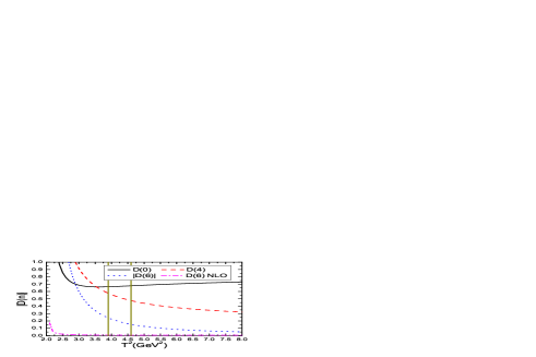
Figure 1: The contributions of the condensates for the hybrid state with the $J^{PC}=1^{-+}$ from the current $J^{V}_{\mu}(x)$, where the two vertical lines denote the Borel window.

In Fig.1, we plot the contributions of the vacuum condensates for the hidden-charm hybrid state with the $J^{PC}=1^{-+}$ from the current $J^{V}_{\mu}(x)$, as an example. From the figure, we can see explicitly that the contributions $D(0)>D(4)\gg|D(6)|$ in the Borel window, on the other hand, the contribution of the $D(6)$ of the NLO is about $1\%$, as the vacuum condensates of dimension-8 are originated from the operators of higher-order expansion of the full heavy quark propagator, see Eq.(24), and companied with the powers $g_{s}^{4}$ and $g_{s}^{5}$, and their contributions are of the NLO [65], and thus they can be neglected safely. The convergent behaviors of the operator product expansion are very good.

In Fig.2, we plot the mass of the hidden-charm hybrid state with the $J^{PC}=1^{-+}$ from the current $J^{V}_{\mu}(x)$ in the cases of different truncations of the operator product expansion, as an example. From the figure, we can see explicitly that the NLO contributions can be absorbed into the pole residue safely, and result in almost degenerated mass, while the LO contributions of dimension-6 play an important role and affect the predicted mass significantly beyond the pole residue.

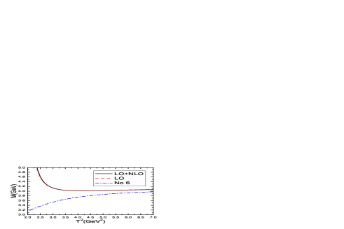
Figure 2: The mass of the hidden-charm hybrid state with the $J^{PC}=1^{-+}$ from the current $J^{V}_{\mu}(x)$, where the ”No 6” denotes the contributions of the condensates of dimension-6 are not included.

Finally, we take account of uncertainties of all input parameters and obtain the masses and pole residues of the hidden-charm hybrid states, which are shown explicitly in Table 2. From Tables 1–2, we can observe explicitly that the energy scale formula, see Eq.(32), is satisfied very good.

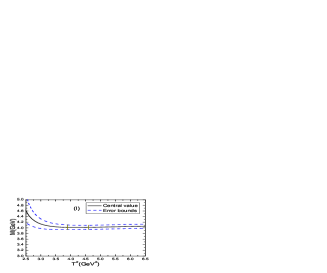
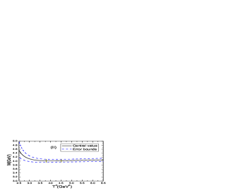
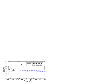
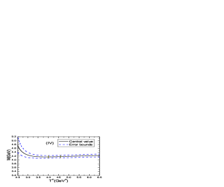
Figure 3: The masses of the hidden-charm hybrid states, where the (I), (II), (III) and (IV) denote the hybrid states with the $J^{PC}=1^{-+}$, $1^{-+}$, $1^{--}$ and $0^{-+}$ from the currents $J_{\mu}^{V}$, $J_{\mu\nu}^{\sigma,0/5}$, $J^{5}_{\mu\nu}$ and $J^{P}$, respectively, the two vertical lines denote the Borel windows.

In Fig.3, we plot the masses of the hidden-charm hybrid states with the $J^{PC}=1^{-+}$, $1^{-+}$, $1^{--}$ and $0^{-+}$ from the currents $J_{\mu}^{V}$, $J_{\mu\nu}^{\sigma,0/5}$, $J^{5}_{\mu\nu}$ and $J^{P}$ respectively with variations of the Borel parameters, as an example. From the figure, we can see explicitly that there really appear elegant platforms in the Borel windows, the uncertainties come from the Borel parameters are rather small. In fact, we can choose larger Borel parameters at the cost of smaller pole contributions, thus we obtain more flatter platforms and better convergent behavior in the operator product expansion, see Figs.1-3. Compared with Ref.[33], we choose larger pole contributions, in fact, only the representation in Ref.[33] is convenient to compare with.

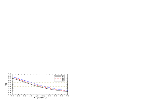
Figure 4: The pole contribution of the hybrid state with the $J^{PC}=1^{-+}$ from the current $J^{V}_{\mu}(x)$, where the $A$, $B$ and $C$ denote the continuum threshold parameters $\sqrt{s_{0}}=4.5\,\rm{GeV}$, $4.6\,\rm{GeV}$ and $4.7\,\rm{GeV}$, respectively.

In Fig.4, we plot the pole contribution of the hidden-charm hybrid state with the $J^{PC}=1^{-+}$ from the current $J^{V}_{\mu}(x)$. From the figure, we can see explicitly that the pole contribution decreases monotonically with increase of the Borel parameter, at the value larger than $4.5\,\rm{GeV}^{2}$, the upper bound of the Borel parameter, the pole contribution is smaller than $40\%$. Although the operator product expansion converge better, see Fig.1, we prefer larger pole contributions, $(40-60)\%$, in an uniform way, and expect to obtain robust predictions.

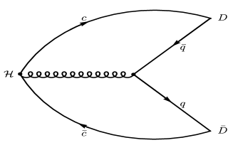
Figure 5: The Feynman diagram for the decays of the hidden-charm hybrid states.

In Fig.5, we draw the Feynman diagram for the decays of the hidden-charm hybrid states, where the $H$ denotes the hidden-charm hybrid states, the light quarks $q=u$, $d$, $s$, the $D$ denotes the charmed mesons $D$, $D_{s}$, $D^{*}$, $D_{s}^{*}$, $D_{0}$, $D_{s0}$, $D_{1}$, $D_{s1}$, $D_{2}$ and $D_{s2}$. We can take the pole residues $\lambda_{H}$, see Table 2, as input parameters to explore the strong decays of those hidden-charm hybrid states with the three-point QCD sum rules, and obtain ratios among the partial decay widths to diagnose their nature. At the present time, the experimental data on the hidden-charm hybrid states are vague, if there really exist a hybrid state with the $J^{PC}=1^{-+}$ at about $4.0\,\rm{GeV}$, see Table 2, then the LHCb’s new state $X(4630)$ can be assigned as the first radial excitation [8].

Currents	$J^{PC}$	$T^{2}(\rm{GeV}^{2})$	$\sqrt{s_{0}}(\rm GeV)$	$\mu(\rm{GeV})$	pole
$J^{P}$	$0^{-+}$	$4.0-4.6$	$4.75\pm 0.10$	$2.0$	$(41-60)\%$
$J^{S}$	$0^{++}$	$6.3-7.6$	$5.75\pm 0.10$	$3.6$	$(40-61)\%$
$J^{V}_{\mu}$	$0^{++}$	$7.4-9.0$	$6.05\pm 0.10$	$3.9$	$(40-60)\%$
$J^{A}_{\mu}$	$0^{--}$	$7.8-9.5$	$6.45\pm 0.10$	$4.5$	$(40-60)\%$
$J^{V}_{\mu}$	$1^{-+}$	$3.9-4.6$	$4.60\pm 0.10$	$1.7$	$(40-61)\%$
$J_{\mu\nu}^{\sigma,0/5}$	$1^{-+}$	$3.8-4.5$	$4.60\pm 0.10$	$1.7$	$(40-61)\%$
$J_{\mu\nu}^{\sigma,0/5}$	$1^{++}$	$6.0-7.3$	$5.60\pm 0.10$	$3.4$	$(40-61)\%$
$J_{\mu\nu}^{0}$	$1^{+-}$	$4.8-5.7$	$5.00\pm 0.10$	$2.4$	$(40-61)\%$
$J^{A}_{\mu}$	$1^{+-}$	$5.6-6.7$	$5.40\pm 0.10$	$3.1$	$(40-60)\%$
$J_{\mu\nu}^{5}$	$1^{+-}$	$6.6-8.0$	$5.85\pm 0.10$	$3.7$	$(40-60)\%$
$J_{\mu\nu}^{5}$	$1^{--}$	$4.3-5.1$	$4.65\pm 0.10$	$1.8$	$(41-61)\%$
$J_{\mu\nu}^{0}$	$1^{--}$	$7.3-8.8$	$6.30\pm 0.10$	$4.3$	$(40-60)\%$
$J_{\mu\nu}^{2,\sigma,5}$	$2^{-+}$	$4.4-5.2$	$4.90\pm 0.10$	$2.3$	$(40-61)\%$
$J_{\mu\nu}^{2,\sigma,0}$	$2^{++}$	$5.6-6.7$	$5.45\pm 0.10$	$3.2$	$(40-60)\%$

Table 1: The Borel windows, continuum threshold parameters, energy scales and pole contributions for the hidden-charm hybrid states.

Currents	$J^{PC}$	$M_{H}(\rm{GeV})$	$\lambda_{H}(\rm{GeV}^{4})$
$J^{P}$	$0^{-+}$	$4.17\pm 0.08$	$1.97\pm 0.22$
$J^{S}$	$0^{++}$	$5.10\pm 0.06$	$5.74\pm 0.44$
$J^{V}_{\mu}$	$0^{++}$	$5.37\pm 0.06$	$2.05\pm 0.14$
$J^{A}_{\mu}$	$0^{--}$	$5.79\pm 0.06$	$2.01\pm 0.14$
$J^{V}_{\mu}$	$1^{-+}$	$4.02\pm 0.08$	$(6.18\pm 0.64)\times 10^{-1}$
$J_{\mu\nu}^{\sigma,0/5}$	$1^{-+}$	$4.01\pm 0.08$	$(5.80\pm 0.62)\times 10^{-1}$
$J_{\mu\nu}^{\sigma,0/5}$	$1^{++}$	$4.96\pm 0.06$	$1.68\pm 0.14$
$J_{\mu\nu}^{0}$	$1^{+-}$	$4.36\pm 0.09$	$(4.31\pm 0.40)\times 10^{-1}$
$J^{A}_{\mu}$	$1^{+-}$	$4.76\pm 0.07$	$1.32\pm 0.11$
$J_{\mu\nu}^{5}$	$1^{+-}$	$5.21\pm 0.07$	$1.12\pm 0.08$
$J_{\mu\nu}^{5}$	$1^{--}$	$4.07\pm 0.10$	$(4.37\pm 0.40)\times 10^{-1}$
$J_{\mu\nu}^{0}$	$1^{--}$	$5.61\pm 0.07$	$1.21\pm 0.09$
$J_{\mu\nu}^{2,\sigma,5}$	$2^{-+}$	$4.31\pm 0.08$	$1.24\pm 0.12$
$J_{\mu\nu}^{2,\sigma,0}$	$2^{++}$	$4.85\pm 0.06$	$2.14\pm 0.18$

Table 2: The masses and pole residues of the hidden-charm hybrid states.

4 Conclusion

In this work, we extend our previous works on the hidden-charm tetraquark (molecular) states and pentaquark (molecular) states to study the hidden-charm hybrid states with the quantum numbers $J^{PC}=0^{-+}$, $0^{++}$, $0^{--}$, $1^{++}$, $1^{+-}$, $1^{-+}$, $1^{--}$, $2^{-+}$ and $2^{++}$ via the QCD sum rules in an systematic way. We calculate the vacuum condensates up to dimensions six in a consistent way by taking account of both the leading-order and next-to-leading order contributions, and take the energy scale formula $\mu=\sqrt{M^{2}_{X/Y/Z}-(2{\mathbb{M}}_{c})^{2}}$ to choose the best energy scales of the QCD spectral densities, it is the first time to explore the energy scale dependence of the QCD sum rules for the hidden-charm hybrid states. Finally, we obtain the mass spectrum, which can be confronted to experimental data in the future. While the pole residues can be taken as input parameters to study the two-body strong decays of the hidden-charm hybrid states with the three-point QCD sum rules.

References

- [1] S. K. Choi et al, Phys. Rev. Lett. 91 (2003) 262001.
- [2] S. Navas et al, Phys. Rev. D110 (2024) 030001.
- [3] E. Kou, and O. Pene, Phys. Lett. B631 (2005) 164.
- [4] S. L. Olsen, T. Skwarnicki and D. Zieminska, Rev. Mod. Phys. 90 (2018) 015003.
- [5] S. L. Zhu, Phys. Lett. B625 (2005) 212.
- [6] Z. G. Wang, Eur. Phys. J. C63 (2009) 115.
- [7] N. Mahajan, Phys. Lett. B679 (2009) 228.
- [8] R. Aaij et al, Phys. Rev. Lett. 127 (2021) 082001.
- [9] Z. G. Wang, Nucl. Phys. B1002 (2024) 116514.
- [10] Z. G. Wang, Adv. High Energy Phys. 2021 (2021) 4426163.
- [11] N. Brambilla, W. K. Lai, A. Mohapatra and A. Vairo, Phys. Rev. D107 (2023) 054034.
- [12] M. Ablikim et al, Phys. Rev. Lett. 129 (2022) 192002.
- [13] H. X. Chen, N. Su and S. L. Zhu, Chin. Phys. Lett. 39 (2022) 051201.
- [14] L. Qiu and Q. Zhao, Chin. Phys. C46 (2022) 051001.
- [15] V. Shastry, C. S. Fischer and F. Giacosa, Phys. Lett. B834 (2022) 137478.
- [16] R. L. Jaffe and K. Johnson, Phys. Lett. B60 (1976) 201.
- [17] T. Barnes, F. E. Close and F. de Viron, Nucl. Phys. B224 (1983) 241.
- [18] M. S. Chanowitz and S. R. Sharpe, Nucl. Phys. B222 (1983) 211.
- [19] D. Horn and J. Mandula, Phys. Rev. D17 (1978) 898.
- [20] N. Isgur, R. Kokoski and J. Paton, Phys. Rev. Lett. 54 (1985) 869.
- [21] F. E. Close and P. R. Page, Nucl. Phys. B443 (1995) 233.
- [22] P. R. Page, E. S. Swanson and A. P. Szczepaniak, Phys. Rev. D59 (1999) 034016.
- [23] J. Govaerts, F. de Viron, D. Gusbin and J. Weyers, Nucl. Phys. B248 (1984) 1.
- [24] J. Govaerts, L. J. Reinders, H. R. Rubinstein and J. Weyers, Nucl. Phys. B258 (1985) 215.
- [25] J. Govaerts, L. J. Reinders and J. Weyers, Nucl. Phys. B262 (1985) 575.
- [26] J. Govaerts, L. J. Reinders, P. Francken, X. Gonze and J. Weyers, Nucl. Phys. B284 (1987) 674.
- [27] T. Huang, H. Y. Jin and A. L. Zhang, Eur. Phys. J. C8 (1999) 465.
- [28] K. G. Chetyrkin and S. Narison, Phys. Lett. B485 (2000) 145.
- [29] H. Y. Jin, J. G. Korner and T. G. Steele, Phys. Rev. D67 (2003) 014025.
- [30] S. Narison, Phys. Lett. B675 (2009) 319.
- [31] C. F. Qiao, L. Tang, G. Hao and X. Q. Li, J. Phys. G39 (2012) 015005.
- [32] D. Harnett, R. T. Kleiv, T. G. Steele and H. Y. Jin, J. Phys. G39 (2012) 125003.
- [33] W. Chen, R. T. Kleiv, T. G. Steele, B. Bulthuis, D. Harnett, J. Ho, T. Richards and S. L. Zhu, JHEP 09 (2013) 019.
- [34] W. Chen, T. G. Steele and S. L. Zhu, J. Phys. G41 (2014) 025003.
- [35] Z. R. Huang, H. Y. Jin and Z. F. Zhang, JHEP 04 (2015) 004.
- [36] A. Palameta, D. Harnett and T. G. Steele, Phys. Rev. D98 (2018) 074014.
- [37] B. Barsbay, K. Azizi and H. Sundu, Eur. Phys. J. C82 (2022) 1086.
- [38] C. M. Tang, Y. C. Zhao and L. Tang, Phys. Rev. D105 (2022) 114004.
- [39] Q. N. Wang, D. K. Lian and W. Chen, Phys. Rev. D108 (2023) 114010.
- [40] A. Alaakol, S. S. Agaev, K. Azizi and H. Sundu, Phys. Lett. B854 (2024) 138711.
- [41] W. H. Tan, N. Su and H. X. Chen, Phys. Rev. D110 (2024) 034031.
- [42] C. M. Tang, C. G. Duan and L. Tang, arXiv: 2411.11433 [hep-ph].
- [43] L. Liu et al, JHEP 07 (2012) 126.
- [44] G. K. C. Cheung, C. O’Hara, G. Moir, M. Peardon, S. M. Ryan, C. E. Thomas and D. Tims, JHEP 12 (2016) 089.
- [45] S. M. Ryan and D. J. Wilson, JHEP 02 (2021) 214.
- [46] A. J. Woss, J. J. Dudek, R. G. Edwards, C. E. Thomas and D. J. Wilson, Phys. Rev. D103 (2021) 054502.
- [47] F. Chen, X. Jiang, Y. Chen, M. Gong, Z. Liu, C. Shi and W. Sun, Phys. Rev. D107 (2023) 054511.
- [48] N. Brambilla, W. K. Lai, J. Segovia, J. T. Castella and A. Vairo, Phys. Rev. D99 (2019) 014017.
- [49] J. Soto and S. T. Valls, Phys. Rev. D108 (2023) 014025.
- [50] Z. G. Wang and T. Huang, Phys. Rev. D89 (2014) 054019.
- [51] Z. G. Wang, Eur. Phys. J. C74 (2014) 2874.
- [52] Z. G. Wang and T. Huang, Nucl. Phys. A930 (2014) 63.
- [53] Z. G. Wang and Q. Xin, Nucl. Phys. B978 (2022) 115761.
- [54] Z. G. Wang, Phys. Rev. D102 (2020) 014018.
- [55] Z. G. Wang, Nucl. Phys. B1007 (2024) 116661.
- [56] Z. G. Wang, Chin. Phys. C48 (2024) 103103.
- [57] Z. G. Wang, Nucl. Phys. B973 (2021) 115592.
- [58] Z. G. Wang, Eur. Phys. J. C79 (2019) 489.
- [59] Z. G. Wang, Int. J. Mod. Phys. A36 (2021) 2150107.
- [60] Z. G. Wang and Z. H. Yan, Eur. Phys. J. C78 (2018) 19.
- [61] Q. Xin and Z. G. Wang, Eur. Phys. J. A58 (2022) 110.
- [62] Z. G. Wang, Int. J. Mod. Phys. A35 (2020) 2050003.
- [63] X. W. Wang, Z. G. Wang, G. L. Yu and Q. Xin, Sci. China-Phys. Mech. Astron. 65 (2022) 291011.
- [64] M. A. Shifman, A. I. Vainshtein and V. I. Zakharov, Nucl. Phys. B147 (1979) 385; Nucl. Phys. B147 (1979) 448.
- [65] L. J. Reinders, H. Rubinstein and S. Yazaki, Phys. Rept. 127 (1985) 1.
- [66] S. Narison and R. Tarrach, Phys. Lett. B125 (1983) 217.
- [67] P. Colangelo and A. Khodjamirian, hep-ph/0010175.
- [68] S. Narison, Nucl. Part. Phys. Proc. 324-329 (2023) 94.
- [69] S. Narison, Nucl. Part. Phys. Proc. 343 (2024) 104.