Symmetric instability in a Boussinesq fluid on a rotating planet

Abstract

Symmetric instability has broad applications in geophysical fluid dynamics. It plays a crucial role in the formation of mesoscale rainbands at mid-latitudes on Earth, instability in the ocean’s mixed layer, and slantwise convection on gas giants and in the oceans of icy moons. Here, we apply linear instability analysis to an arbitrary zonally symmetric Boussinesq flow on a rotating spherical planet, with applicability to planetary atmospheres and icy moon oceans. We characterize the instabilities into three types: (1) gravitational instability, occurring when stratification is unstable along angular momentum surfaces, (2) inertial instability, occurring when angular momentum shear is unstable along buoyancy surfaces, and (3) a mixed “PV” instability, occurring when the potential vorticity has the opposite sign as planetary rotation. We note that $N^{2}>0$, where $N$ is the Brunt-Väisälä frequency, is neither necessary nor sufficient for stability. Instead, $b_{z}\sin{\theta}>0$, where $b_{z}$ is the stratification along the planetary rotation axis and $\theta$ is latitude, is always necessary for stability and also sufficient in the low Rossby number limit. In the low Rossby number limit, applicable to convection in the oceans of icy moons and in the atmospheres of gas giants, the most unstable mode is slantwise convection parallel to the planetary rotation axis.

1 Introduction

Symmetric instability describes the instability of axisymmetric flow. In an axisymmetric rotating fluid with background density stratification and angular momentum gradient, if a fluid parcel is perturbed from its origin, two restoring forces come into play: the buoyancy force and the inertial acceleration (Coriolis and centrifugal forces). These forces individually may result in gravitational instability or inertial instability. Moreover, even when the fluid is both gravitationally and inertially stable, the combined effects of the two force anomalies may cause the parcel to deviate further from its origin, resulting in symmetric instability (Hoskins, 1974; Haine & Marshall, 1998).

Symmetric instability has broad applications in geophysical fluid dynamics. On Earth, it is relevant to the formation of mesoscale rainbands in the midlatitude atmosphere (e.g., Emanuel, 1983, 1985) and instability in the ocean’s mixed layer (e.g., Straneo et al., 2002; Callies & Ferrari, 2018). Beyond Earth, symmetric instability is closely tied to slantwise convection in the atmospheres of gas giants (e.g., Stone, 1967; Busse, 1970; Stone, 1971; Walton, 1975; O’Neill & Kaspi, 2016) and in the oceans of their icy satellites (e.g., Soderlund, 2019; Kang et al., 2022; Bire et al., 2022; Zeng & Jansen, 2024), where convection is tilted along angular momentum surfaces.

Symmetric instability is often studied in gravitationally and inertially stable fluids, where it occurs when the planetary vorticity has a different sign from the potential vorticity. In the Northern Hemisphere, symmetric instability happens when the potential vorticity $q=\nabla b\cdot(2\mathbf{\Omega}+\nabla\times\mathbf{v})$ is negative, where $\mathbf{\Omega}$ is the planetary rotation and $\mathbf{v}$ is the 3-dimensional (3-D) relative velocity in the rotating frame (Eliassen, 1951; Ooyama, 1966; Hoskins, 1974; Stevens, 1983). The instability criteria can be expressed in terms of the Richardson number, $Ri=N^{2}/(\partial u/\partial R)^{2}$ where $N^{2}=-(g/\rho)(\partial\rho/\partial R)$ is the stratification parallel to gravity, $g$ is gravity, $\rho$ is density, $u$ is the zonal component of the velocity, and $\partial/\partial R$ denotes the derivative along the gravitational direction. On an $f$-plane where we only consider the planetary rotation parallel to gravity ($f=2\Omega\sin{\theta}$ with $\theta\in(-\pi/2,\pi/2]$ denoting latitude), under the assumption of gravitational stability ($N^{2}>0$) and inertial stability ($\eta/f>0$), where $\eta=f-(1/R)(\partial u/\partial\theta)$ is the absolute vorticity with $R$ denoting the planetary radius, symmetric instability occurs when $Ri<\eta/f$ (c.f. Hoskins, 1974; Haine & Marshall, 1998). Later studies have considered a “tilted $f$-plane” that takes into account both vertical and horizontal components of the planetary rotation, $\mathbf{f}=f\mathbf{e_{R}}+\tilde{f}\mathbf{e_{\theta}}$ where $\tilde{f}=2\Omega\cos{\theta}$, $\mathbf{e_{R}}$ denotes the upwards direction parallel to gravity, and $\mathbf{e_{\theta}}$ denotes the latitudinal direction (Sun, 1995; Straneo et al., 2002; Fruman & Shepherd, 2008; Itano & Maruyama, 2009; Jeffery & Wingate, 2009). Sun (1995) concluded that as latitude decreases, i.e., the angle between planetary rotation and gravity becomes larger, the effect of $\tilde{f}$ in modulating the maximum growth rate of symmetric instability increases. Itano & Maruyama (2009) finds that the parameter regime for the occurrence of symmetric instability is less sensitive to $\tilde{f}$ when $Ri>0.25$ and $\eta/f>1$, but is considerably influenced in other regions.

Most studies on symmetric instability assume stable stratification in the gravitational direction, $N^{2}>0$, a priori. However, although $N^{2}>0$ is a reasonable assumption in most regions of Earth’s atmosphere and ocean, it may not hold on other planetary bodies such as icy moon oceans and gas giant atmospheres. In studies focusing on rotating convective instability, scenarios with $N^{2}<0$ have been considered (e.g., Flasar & Gierasch, 1978; Hathaway et al., 1979), and it has been shown that the system can remain stable even when $N^{2}<0$ (see Figure 2 in Hathaway et al. (1979)). In Flasar & Gierasch (1978) and Hathaway et al. (1979), the background shear is assumed to be purely vertical. However, meridional shears are likely to be important in the oceans of icy moons and the atmospheres of gas giants (Kaspi et al., 2009; Bire et al., 2022).

In this paper, we seek to explore symmetric instability in a generalized parameter regime applicable to deep planetary atmospheres and oceans with arbitrary vertical and meridional shears. We apply a linear instability analysis to the adiabatic, inviscid, nonhydrostatic Boussinesq equations formulated in cyclindrical coordinates, keeping all Coriolis and metric terms. We linearize around a zonally symmetric background state in hydrostatic and gradient wind balance, but make no further assumptions about this state. In particular, we do not require the background stratification to be stable in the gravitational direction ($N^{2}>0$), which, as we show, is in general neither a necessary nor sufficient condition for stability. In section 2, the theoretical analysis for linear instability criteria, the most unstable mode, and the maximum growth rate are discussed. Section 3 presents the numerical simulation results for comparison with the theoretical analysis. Section 4 provides the discussion and concluding remarks.

2 Linear instability analysis

2.1 Instability criteria

The adiabatic, inviscid, nonhydrostatic equations for a Boussinesq fluid are:

$$\frac{D\mathbf{v}}{Dt}+2\mathbf{\Omega}\times\mathbf{v}=-\nabla\Phi+\frac{\rho^{\prime}}{\rho_{0}}\mathbf{g},$$ (1)

$$\nabla\cdot\mathbf{v}=0,$$ (2)

$$\frac{D\rho^{\prime}}{Dt}=0.$$ (3)

where $\Phi=p^{\prime}/\rho_{0}$, $p^{\prime}$ is the pressure anomaly, $\rho_{0}$ is the reference density, $\mathbf{g}$ is the gravity, and $\rho^{\prime}$ is the density anomaly (c.f. Vallis, 2017). By writing the equations in cylindrical coordinates $(\mathbf{e_{r}},\mathbf{e_{\phi}},\mathbf{e_{z}})$ where $\mathbf{e_{r}}$ is the radial direction, $\mathbf{e_{\phi}}$ is the zonal (azimuthal) direction, and $\mathbf{e_{z}}$ is the vertical (rotational) direction ($\mathbf{\Omega}=\Omega\mathbf{e_{z}}$), we have

$$\left(\frac{\partial}{\partial t}+\frac{u}{r}\frac{\partial}{\partial\phi}+v\frac{\partial}{\partial r}+w\frac{\partial}{\partial z}\right)u+2\Omega v+\frac{uv}{r}=-\frac{1}{r}\frac{\partial\Phi}{\partial\phi},$$ (4)

$$\left(\frac{\partial}{\partial t}+\frac{u}{r}\frac{\partial}{\partial\phi}+v\frac{\partial}{\partial r}+w\frac{\partial}{\partial z}\right)v-2\Omega u-\frac{u^{2}}{r}=-\frac{\partial\Phi}{\partial r}+b\cos{\theta},$$ (5)

$$\left(\frac{\partial}{\partial t}+\frac{u}{r}\frac{\partial}{\partial\phi}+v\frac{\partial}{\partial r}+w\frac{\partial}{\partial z}\right)w=-\frac{\partial\Phi}{\partial z}+b\sin{\theta},$$ (6)

$$\left(\frac{\partial}{\partial t}+\frac{u}{r}\frac{\partial}{\partial\phi}+v\frac{\partial}{\partial r}+w\frac{\partial}{\partial z}\right)b=0,$$ (7)

$$\frac{1}{r}\frac{\partial u}{\partial\phi}+\frac{\partial v}{\partial r}+\frac{\partial w}{\partial z}+\frac{v}{r}=0,$$ (8)

where $\mathbf{v}=u\mathbf{e_{\phi}}+v\mathbf{e_{r}}+w\mathbf{e_{z}}$ are the velocity components, $r$ is the local radius (distance to the planetary rotational axis), and $b=-g\rho^{\prime}/\rho_{0}$ is buoyancy. We consider an axisymmetric state around the planetary rotation axis where all variables are invariant in the zonal direction ($\partial/\partial\phi=0$, i.e. zonally symmetric), and assume a background state with an arbitrary background zonal flow $u_{0}(r,z)$ and buoyancy field $b_{0}(r,z)$ that are invariant in time:

$$\mathbf{v}=u_{0}(r,z)\mathbf{e_{\phi}}+\mathbf{v^{\prime}}(r,z,t),\ \ b=b_{0}(r,z)+b^{\prime}(r,z,t),\ \ \Phi=\Phi_{0}(r,z)+\Phi^{\prime}(r,z,t).$$ (9)

Assuming the perturbations are small, the zeroth-order balance reveals the gradient wind balance and hydrostatic balance for the background state:

$$-2\Omega u_{0}-\frac{u_{0}^{2}}{r}=-\frac{\partial\Phi_{0}}{\partial r}+b_{0}\cos{\theta},$$ (10)

$$0=-\frac{\partial\Phi_{0}}{\partial z}+b_{0}\sin{\theta}.$$ (11)

With

$$f_{0}=2\Omega+\frac{2u_{0}}{r},$$ (12)

being a modified Coriolis parameter describing the effect of planetary rotation and centrifugal force, Equations 10 & 11 yield

$$f_{0}\frac{\partial u_{0}}{\partial z}=b_{r}\sin{\theta}-b_{z}\cos{\theta},$$ (13)

where $b_{r}=\partial b_{0}/\partial r$ and $b_{z}=\partial b_{0}/\partial z$ are the background buoyancy gradients. Equation 13 is similar to the thermal wind balance in a rapidly rotating (geostrophic) fluid (Kaspi et al., 2009; Bire et al., 2022), although $f_{0}$ is here modulated by the background flow.

In the first-order balance, we have the linearized perturbation equations:

$$\frac{\partial u^{\prime}}{\partial t}+\left(2\Omega+\frac{\partial u_{0}}{\partial r}+\frac{u_{0}}{r}\right)v^{\prime}+\frac{\partial u_{0}}{\partial z}w^{\prime}=0,$$ (14)

$$\frac{\partial v^{\prime}}{\partial t}-\left(2\Omega+\frac{2u_{0}}{r}\right)u^{\prime}-\cos{\theta}b^{\prime}+\frac{\partial\Phi^{\prime}}{\partial r}=0,$$ (15)

$$\frac{\partial w^{\prime}}{\partial t}-\sin{\theta}b^{\prime}+\frac{\partial\Phi^{\prime}}{\partial z}=0,$$ (16)

$$\frac{\partial b^{\prime}}{\partial t}+b_{r}v^{\prime}+b_{z}w^{\prime}=0,$$ (17)

$$\frac{1}{r}\frac{\partial(v^{\prime}r)}{\partial r}+\frac{\partial w^{\prime}}{\partial z}=0.$$ (18)

Defining radius-weighted velocity and buoyancy fields as $\tilde{u}=u^{\prime}r$, $\tilde{v}=v^{\prime}r$, $\tilde{w}=w^{\prime}r$, and $\tilde{b}=b^{\prime}r$, the perturbation equations become:

$$\frac{\partial\tilde{u}}{\partial t}+M_{r}\tilde{v}+M_{z}\tilde{w}=0,$$ (19)

$$\frac{\partial\tilde{v}}{\partial t}-f_{0}\tilde{u}-\cos{\theta}\tilde{b}+r\frac{\partial\Phi^{\prime}}{\partial r}=0,$$ (20)

$$\frac{\partial\tilde{w}}{\partial t}-\sin{\theta}\tilde{b}+r\frac{\partial\Phi^{\prime}}{\partial z}=0,$$ (21)

$$\frac{\partial\tilde{b}}{\partial t}+b_{r}\tilde{v}+b_{z}\tilde{w}=0,$$ (22)

$$\frac{\partial\tilde{v}}{\partial r}+\frac{\partial\tilde{w}}{\partial z}=0,$$ (23)

where

$$M_{r}=\frac{1}{r}\frac{\partial}{\partial r}\left(\Omega r^{2}+u_{0}r\right)=2\Omega+\frac{u_{0}}{r}+\frac{\partial u_{0}}{\partial r},\quad M_{z}=\frac{1}{r}\frac{\partial}{\partial z}\left(\Omega r^{2}+u_{0}r\right)=\frac{\partial u_{0}}{\partial z}$$ (24)

describe the radial and vertical gradients of the background angular momentum $m=\Omega r^{2}+u_{0}r$.

We look for local plane-wave solutions:

$$(\tilde{u},\tilde{v},\tilde{w},\tilde{b},\Phi^{\prime})=(A_{u},A_{v},A_{w},A_{b},A_{\Phi})\exp(ik_{r}r+ik_{z}z-i\omega t),$$ (25)

where $A_{u},A_{v},A_{w},A_{b},A_{\Phi}$ are constant amplitudes, $k_{r}$ and $k_{z}$ are radial and vertical wave numbers, and $\omega$ is the frequency. Substituting Equation 25 into Equations 19-23, we get a linearized equation system. The linearized equations must have zero determinant to have non-trival solutions, which requires

$$\left|\begin{matrix}-i\omega&M_{r}&M_{z}&0&0\\ -f_{0}&-i\omega&0&-\cos{\theta}&ik_{r}r\\ 0&0&-i\omega&-\sin{\theta}&ik_{z}r\\ 0&b_{r}&b_{z}&-i\omega&0\\ 0&ik_{r}&ik_{z}&0&0\\ \end{matrix}\right|=0.$$ (26)

This gives

$$r\omega[(k_{r}^{2}+k_{z}^{2})\omega^{2}-b_{z}\sin{\theta}k_{r}^{2}-(f_{0}M_{r}+b_{r}\cos{\theta})k_{z}^{2}+2b_{r}\sin{\theta}k_{r}k_{z}]=0.$$ (27)

Neglecting the trivial solutions $\omega=0$ and $k_{r}=k_{z}=0$, we have the dispersion relation:

$$\omega^{2}=\frac{b_{z}\sin{\theta}k_{r}^{2}+(f_{0}M_{r}+b_{r}\cos{\theta})k_{z}^{2}-2b_{r}\sin{\theta}k_{r}k_{z}}{k_{r}^{2}+k_{z}^{2}}.$$ (28)

Stability requires that the frequency $\omega$ has no imaginary part, which means the right-hand-side of Equation 28 is positive definite. Specifically, this requires the quadratic function $b_{z}\sin{\theta}k_{r}^{2}+(f_{0}M_{r}+b_{r}\cos{\theta})k_{z}^{2}-2b_{r}\sin{\theta}k_{r}k_{z}>0$ for all $k_{r}$ and $k_{z}$. Consequently, the stability matrix

$$\left(\begin{matrix}b_{z}\sin{\theta}&-b_{r}\sin{\theta}\\ -b_{r}\sin{\theta}&f_{0}M_{r}+b_{r}\cos{\theta}\\ \end{matrix}\right)$$ (29)

must be positive definite. Therefore, the necessary and sufficient conditions for instability are that either the trace or determinant of this matrix be negative, i.e., either

$$b_{z}\sin{\theta}+f_{0}M_{r}+b_{r}\cos{\theta}<0,$$ (30)

or

$$b_{z}\sin{\theta}(f_{0}M_{r}+b_{r}\cos{\theta})-b_{r}^{2}\sin^{2}{\theta}<0.$$ (31)

Equation 31 can also be expressed in terms of a condition for the background potential vorticity. The background potential vorticity is

$$q=\nabla b_{0}\cdot(2\mathbf{\Omega}+\nabla\times\mathbf{v_{0}})=M_{r}b_{z}-M_{z}b_{r}=M_{r}b_{z}-\frac{b_{r}}{f_{0}}(b_{r}\sin{\theta}-b_{z}\cos{\theta}),$$ (32)

where the background gradient wind shear equation (13) is applied. We can hence rewrite Equation 31 as

$$qf_{0}\sin{\theta}<0,$$ (33)

i.e. instability occurs if the potential vorticity has the opposite sign as the generalized background planetary vorticity (Equation 32). It is worth noting here that the PV criterion (Equation 33) by itself is a sufficient but not necessary condition for instability.

2.2 Most unstable mode and growth rate

When $\omega$ is imaginary ($\omega=i\sigma$), the perturbation fields will grow exponentially with $\sigma$ being the e-folding growth rate and the system is unstable. Let $\delta\in(-\pi/2,\pi/2]$ be the angle between the unstable mode and $\mathbf{e_{r}}$ so that $\tan{\delta}=-k_{r}/k_{z}$. By substituting $\omega=i\sigma$ in the dispersion relation (Equation 28), the growth rate of the mode can be expressed as

$$\sigma=\left(-\frac{b_{z}\sin{\theta}\tan^{2}{\delta}+2b_{r}\sin{\theta}\tan{\delta}+f_{0}M_{r}+b_{r}\cos{\theta}}{1+\tan^{2}{\delta}}\right)^{1/2}.$$ (34)

Equation 34 indicates that for a given background field and latitude, the growth rate is only a function of $\tan\delta$, i.e. the direction of the unstable mode, but not the magnitude of the wavenumber, i.e. the size of the mode. By calculating the derivatives of the function $\sigma(\tan{\delta})$ and performing some algebra, we find that the maximum growth rate is obtained when

$$\tan{\delta_{m}}=\frac{b_{z}\sin{\theta}-f_{0}M_{r}-b_{r}\cos{\theta}-\left[(b_{z}\sin{\theta}-f_{0}M_{r}-b_{r}\cos{\theta})^{2}+4b_{r}^{2}\sin^{2}{\theta}\right]^{1/2}}{2b_{r}\sin{\theta}}.$$ (35)

Substituting Equation 35 into Equation 34, we obtain the maximum growth rate as

$$\sigma_{m}=\left(\frac{-b_{z}\sin{\theta}-f_{0}M_{r}-b_{r}\cos{\theta}+\sqrt{(f_{0}M_{r}+b_{r}\cos{\theta}-b_{z}\sin{\theta})^{2}+4b_{r}^{2}\sin^{2}{\theta}}}{2}\right)^{1/2}.$$ (36)

2.3 Instability diagram

When $b_{r}\sin{\theta}=0$, the most unstable mode always aligns with the radial ($r$) or vertical ($z$) directions, as discussed in Section 2.5.1 (for $\sin{\theta}=0$) and Appendix A (for $b_{r}=0$). In this section, we discuss the more general case when $b_{r}\sin{\theta}\neq 0$. The instability criteria for displacements purely along the $\mathbf{e_{r}}$ and $\mathbf{e_{z}}$ directions are $f_{0}M_{r}+b_{r}\cos{\theta}<0$ and $b_{z}\sin{\theta}<0$, respectively, which are derived by solving $\omega^{2}<0$ (Equation 28) when $k_{r}=0$ and $k_{z}=0$. We can define a 2-D nondimensionalized phase space based on the stability in these two orthogonal directions:

$$x=\frac{b_{z}\sin{\theta}}{|b_{r}\sin{\theta}|},\ \ y=\frac{f_{0}M_{r}+b_{r}\cos{\theta}}{|b_{r}\sin{\theta}|}.$$ (37)

The stability matrix then becomes

$$\left(\begin{matrix}x&-1\\ -1&y\\ \end{matrix}\right),$$ (38)

and positive definiteness requires that

$$x+y>0,\ \mathrm{and}\ xy>1,$$ (39)

which means only the region above the hyperbolic $xy=1$ in the first quadrant ($x>0$, $y>0$) is stable (Figure 1a).

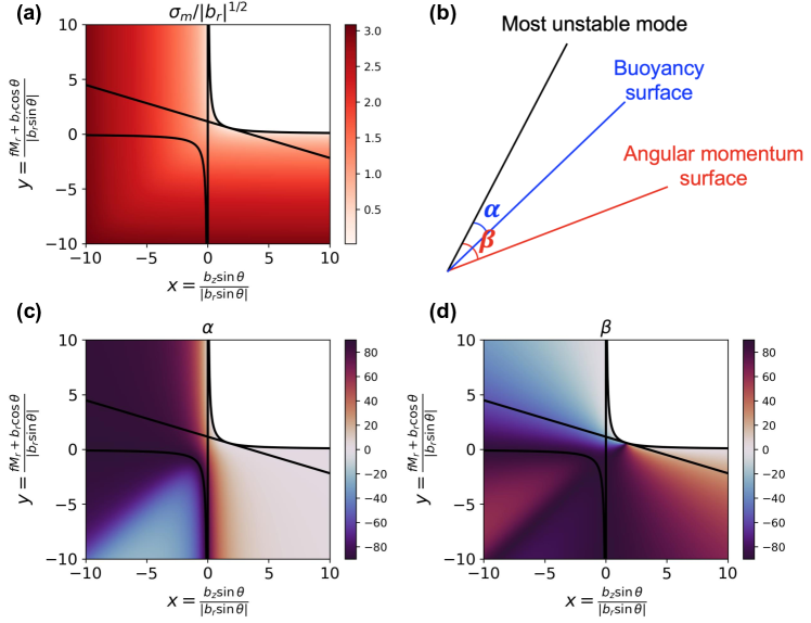
Figure 1: Growth rate and orientation of the most unstable mode with $b_{r}>0$ and $\theta=60^{\circ}$. (a): growth rate of the most unstable mode, non-dimensionalized with $|b_{r}|^{1/2}$: $\sigma_{m}/|b_{r}|^{1/2}=((-x-y+((x-y)^{2}+4)^{1/2})|\sin{\theta}|/2)^{1/2}$. (b): sketch for the definition of $\alpha$ and $\beta$. (c) and (d): the angle (in degrees) between the most unstable mode and the buoyancy surface ($\alpha$, c) and the angular momentum surface ($\beta$, d). In (a), (c) and (d), the solid lines separate the plane into regions where gravitational instability, inertial instability, PV instability, or a combination of them occur (see Figure 2 and discussion in Section 2.4).

2.4 Gravitational instability, inertial instability, and PV instability

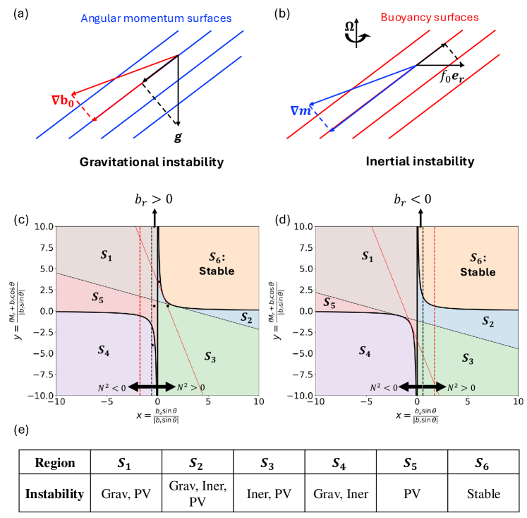
Figure 2: Different types of instabilities and the instability diagram. (a) and (b): sketches for gravitational instability (a) and inertial instability (b), respectively. In (a), gravitational instability occurs if the buoyancy gradient (red arrows) and the gravity (black arrows) are in the same direction when projected onto the angular momentum surfaces (blue lines). In (b), inertial instability occurs when the angular momentum gradient (blue arrows) and $f_{0}\mathbf{e_{r}}$ (black arrows) are in opposite directions when projected onto the buoyancy surfaces (red lines). (c) and (d): instability diagram for $b_{r}>0$ (c) and $b_{r}<0$ (d), respectively. Solid lines indicate gravitational, inertial, and PV instability criteria. The thicker solid lines indicate the hyperbolic curve $xy=1$ (Equation 44) and the line $x=0$ (Equation 42). The thinner solid lines indicate the line $y+\cot^{2}{\theta}x-2|\cot{\theta}|\mathrm{sgn}(b_{r})=0$ (Equation 43). Note that the line $y+\cot^{2}{\theta}x-2|\cot{\theta}|\mathrm{sgn}(b_{r})=0$ is always tangential to the hyperbolic curve $xy=1$. The dashed lines indicate $N^{2}=0$, with regions to the left of these lines corresponding to $N^{2}<0$. The black lines are for $\theta=60^{\circ}$ and red lines are for $\theta=30^{\circ}$ for comparison. The black dots are simulation parameters for $s_{1GP}$ to $s_{6S}$ (Table 1). Note that for $s_{1GP}$ and $s_{6S}$, the $y$-axis value is $1.15\times 10^{4}$, outside the $y$-values shown in the plot. Types of instabilities in different regions are summarized in (e), where “Grav” indicates gravitational instability (Equation 40), “Iner” indicates inertial instability (Equation 41), and “PV” indicates PV instability (Equation 33), respectively.

In a rotating fluid with background stratification and shear, two restoring forces, associated with gravity and rotation, act when a fluid parcel is displaced: buoyancy force and inertial acceleration. If a fluid parcel is displaced along a constant angular momentum surface, the inertial acceleration anomaly is zero and the only restoring force is the buoyancy force anomaly. As a result, pure gravitational instability can occur when the stratification is unstable along constant angular momentum surfaces. Similarly, if the displacement of the fluid parcel is along a constant buoyancy surface, the only restoring force is the inertial acceleration anomaly, hence pure inertial instability can occur when the angular momentum shear is unstable along constant buoyancy surfaces. Here, unstable stratification indicates buoyancy decreases in the opposite direction to $\mathbf{g}$, and unstable angular momentum shear indicates the angular momentum gradient is opposite to $f_{0}\mathbf{e_{r}}$ (Figure 2a & b). Therefore, gravitational instability can occur when

$$(\nabla b_{0}\cdot\mathbf{e_{M}})(-\mathbf{g}\cdot\mathbf{e_{M}})=g(M_{r}b_{z}-M_{z}b_{r})(M_{r}\sin{\theta}-M_{z}\cos{\theta})<0,$$ (40)

where $\mathbf{e_{M}}=-M_{z}\mathbf{e_{r}}+M_{r}\mathbf{e_{z}}$ is the direction along a constant angular momentum surface. Inertial instability can occur when

$$(\nabla m\cdot\mathbf{e_{b}})(f_{0}\mathbf{e_{r}}\cdot\mathbf{e_{b}})=f_{0}b_{z}r^{2}(M_{r}b_{z}-M_{z}b_{r})<0,$$ (41)

where $\mathbf{e_{b}}=-b_{z}\mathbf{e_{r}}+b_{r}\mathbf{e_{z}}$ is the direction along a constant buoyancy surface. Using the gradient wind shear (Equation 13), and the definition of the phase space (Equation 37), Equation 40 becomes

$$[y+\cot^{2}{\theta}x-2|\cot{\theta}|\mathrm{sgn}(b_{r})](xy-1)<0,$$ (42)

where $\mathrm{sgn}$ denotes the sign function, and Equation 41 becomes

$$x(xy-1)<0.$$ (43)

Comparison with the results derived in Section 2.1 shows that neither the gravitational or inertial instability criteria are necessary for instability. Instability can still occur when the potential vorticity takes a different sign as planetary rotation. The PV instability criterion (Equation 33) in the nondimensional form is

$$xy-1<0.$$ (44)

In the instability diagram, the phase plane, characterized by the nondimensional parameters $x$ and $y$, is divided into several regions where gravitational instability (Equation 42), inertial instability (Equation 43), or PV instability (Equation 44) occur. In all regions except for the stable region $S_{6}$ located above the hyperbolic curve $xy=1$ in the first quadrant, at least one type of instability is present (see Figure 2c-e).

The alignment of the most unstable mode with the buoyancy and angular momentum surfaces is indicative of different types of instabilities. To illustrate how the most unstable mode aligns with the buoyancy and angular momentum surfaces, we define $\alpha\in(-\pi/2,\pi/2]$ as the angle between the most unstable mode and the buoyancy surface, and $\beta\in(-\pi/2,\pi/2]$ as the angle between the most unstable mode and the angular momentum surface, with the most unstable mode counterclockwise of the buoyancy/angular momentum surface defined as positive (Figure 1b). By comparing Figure 2c and Figure 1c & d, regions where the most unstable mode aligns with the buoyancy surface ($\alpha=0$) can be identified as inertially unstable, and regions where the most unstable mode aligns with the angular momentum surface ($\beta=0$) can be identified as gravitationally unstable. However, the opposite is not always true, and in many parts of the parameter regime, the most unstable mode does not align with either surface. A special case where the Rossby number is small and the most unstable mode aligns with the angular momentum surface will be discussed in Section 2.5.2.

Most previous studies on symmetric instability have neglected regimes where $N^{2}<0$ or $\eta/f<0$, as they typically assume stable stratification in the gravitational direction and stable zonal velocity shear in the latitudinal direction. However, we find that while $\eta/f<0$ is a sufficient condition for instability, $N^{2}<0$ is not sufficient for instability (see detailed derivations in Appendix B). In Figure 2c & d, $N^{2}=0$ is indicated by dashed lines, with regions to the left of these lines corresponding to $N^{2}<0$. Therefore, when $b_{r}<0$, the system can remain stable even if $N^{2}<0$, highlighting that $N^{2}<0$ is neither a necessary nor a sufficient condition for instability.

2.5 Two special limits

2.5.1 The equatorial plane

In Sections 2.3 and 2.4 we assumed that $b_{r}\sin\theta\neq 0$, which excludes the equatorial plane ($\theta=0$). Thus, we discuss the equatorial plane separately here (the case with $b_{r}=0$ is discussed in Appendix A). At the equator, the left-hand-side of the PV criterion (Equation 33) is always zero. The gravitational instability criterion (Equations 40) and the inertial instability criterion (Equation 41) both reduce to

$$f_{0}M_{r}+b_{r}=f_{0}^{2}+f_{0}\frac{\partial u_{0}}{\partial r}+b_{r}<0.$$ (45)

For instability to arise at the equator, either the zonal velocity gradient ($\partial u_{0}/\partial r$) must be comparable and have opposite sign to the planetary rotation $f_{0}$ (shear-driven), or the buoyancy gradient $b_{r}$ must be negative and comparable to $f_{0}^{2}$ (stratification-driven), or some combination thereof. Taking the limit $\theta\to 0$ of Equation 35, we find that the maximum growth rate at the equator is

$$\sigma_{m}=(-f_{0}M_{r}-b_{r})^{1/2}\ \ \mathrm{when}\ \delta_{m}=0,$$ (46)

meaning the most unstable mode aligns with the radial direction, parallel to local gravity, independent of the background shear and stratification.

2.5.2 Low Rossby number limit

In the low Rossby number regime, $Ro=U/(f_{0}L)\ll 1$ where $U$ is the velocity scale and $L$ is the length scale of motion, the rotational effect dominates over nonlinear advection (c.f. Vallis, 2017). Many fluid motions in geophysical fluid dynamics fall into this regime, such as large-scale atmospheric motions outside the equatorial region on gas giants like Jupiter (Kaspi et al., 2018) and the ocean flow on icy moons and Snowball Earth (Jansen et al., 2023). In the low Rossby number limit, we have $u_{0}/r$, $\partial u_{0}/\partial r$, $\partial u_{0}/\partial z\ll f_{0}$, which implies $M_{r}\approx f_{0}\approx 2\Omega$ and $M_{z}\ll f_{0}$. In gradient wind balance, we moreover have the scaling that $b_{r},\ b_{z}\sim f_{0}M_{z}\ll f_{0}^{2}$. Consequently, the criterion for inertial instability, Equation 41, reduces to

$$f_{0}^{2}b_{z}^{2}<0,$$ (47)

which cannot be satisfied, indicating that zonally-symmetric flow with small $Ro$ is always inertially stable (because angular momentum is predominantly controlled by planetary rotation). Instability occurs when

$$b_{z}\sin{\theta}<0,$$ (48)

i.e. for a gravitationally unstable stratification in the direction parallel to planetary rotation, which coincides with the angular momentum surface in the small $Ro$ limit. The most unstable mode (Equation 35) is obtained when

$$\left|\tan{\delta_{m}}\right|\approx\left|\frac{-f_{0}^{2}-[(f_{0}^{2})^{2}]^{1/2}}{2b_{r}\sin{\theta}}\right|=\left|\frac{f_{0}^{2}}{b_{r}\sin{\theta}}\right|\gg 1,\ \ \mathrm{i.e.}\ \delta_{m}\approx\frac{\pi}{2},$$ (49)

and the corresponding growth rate is

$$\sigma_{m}\approx(-b_{z}\sin{\theta})^{1/2}.$$ (50)

Therefore, the most unstable mode is associated with slantwise convection aligned with the planetary angular momentum surface. This mode, parallel to the rotational axis, is likely to be important in the atmospheres of gas giants and in the oceans of icy moons, which are characterized by low Rossby numbers. Observations of the gravitational fields of Jupiter and Saturn suggest that the zonal jets on these gas giants are aligned with the rotational axis (Kaspi et al., 2018; Galanti et al., 2019; Kaspi et al., 2023), indicating that the prevailing modes are parallel to planetary rotation. Numerical simulations of gas giant atmospheres (e.g., Christensen, 2002; Kaspi et al., 2009; Heimpel et al., 2016) and icy moon oceans (e.g., Soderlund, 2019; Kang et al., 2022; Bire et al., 2022; Zeng & Jansen, 2024) have also identified slantwise convection aligned with the rotational axis.

3 Numerical simulations

3.1 Simulation set up

To verify the theoretical results, we numerically integrate Equations 4-8 using Dedalus, which can solve initial-value partial differential equations using spectral methods (Burns et al., 2020). Under the zonally symmetric assumption ($\partial/\partial\phi=0$), the equations reduce to a 2-D system ($r,z$). We prescribe a background state, which satisfies the gradient wind balance (Equations 10 & 11), and solve for the evolution of the perturbation fields ($u^{\prime},v^{\prime},w^{\prime},b^{\prime},\Phi^{\prime}$) under double-periodic boundary conditions to search for solutions in an infinitely large domain. A Cartesian coordinate system is employed to allow for double-periodic boundary conditions, resulting in the neglect of the metric terms ($uv/r$ in Equation 4, $-u^{2}/r$ in Equation 5, and $v/r$ in Equation 8), such that $f_{0}=2\Omega$ and $M_{r}=2\Omega+\partial u_{0}/\partial r$. We non-dimensionalize the equations with the rotational time scale ($T=f_{0}^{-1}$) and the domain length scale. We apply a resolution with 256 grid points in both $r$ and $z$ directions.

We carry out simulations $s_{1GP}$ to $s_{6S}$ with the background field representing regions $S_{1}$ to $S_{6}$ in the parameter space, where different types of instability occur (see Figure 2). Two additional simulations, $s_{7GI}$ and $s_{8GI}$, are conducted to represent the equatorial region, with shear-driven instability in $s_{7GI}$ ($M_{r}<0$) and stratification-driven instability in $s_{8GI}$ ($b_{r}<0$). The simulation parameters are summarized in Table 1 and the prescribed background fields are shown in Figure 3.

Simulation	$\theta$ (∘)	$b_{r}$	$b_{z}$	$M_{r}$	$q$	$N^{2}$	Instability	$\sigma_{m}$
$s_{1GP}$	60∘	$10^{-4}$	$-10^{-4}/3$	$1$	$-3.33\times 10^{-5}$	$2.11\times 10^{-5}$	Grav, PV	$5.37\times 10^{-3}$
$s_{2GIP}$	60∘	$1$	$0.15$	$2.5$	$-0.416$	$0.630$	Grav, Iner, PV	$0.333$
$s_{3IP}$	60∘	$1$	$1$	$0$	$-0.366$	$1.37$	Iner, PV	$0.450$
$s_{4GI}$	60∘	$1$	$-0.5$	$-4$	$0.884$	$6.70\times 10^{-2}$	Grav, Iner	$1.93$
$s_{5P}$	60∘	$1$	$-1/3$	$0$	$-1.03$	$0.211$	PV	$0.920$
$s_{6S}$	60∘	$-10^{-4}$	$10^{-4}/3$	$1$	$3.33\times 10^{-5}$	$-2.11\times 10^{-5}$	Stable	/
$s_{7GI}$	0∘	$1$	$-1$	$-2$	$1$	$1$	Grav, Iner	$1$
$s_{8GI}$	0∘	$-2$	$-1$	$1$	$1$	$-2$	Grav, Iner	$1$

Table 1: Numerical simulation set-ups. The simulation parameters are non-dimensionalized with the rotational time scale ($T=f_{0}^{-1}$ so that the non-dimensionalized $f_{0}$ is 1 in all simulations) and the domain length scale. The types of instability in each simulation are indicated in the simulation name and the “Instability” column, where $G$ and Grav indicate gravitational instability, $I$ and Iner indicate inertial instability, $P$ and PV indicate PV instability, and $S$ and Stable indicate the system is stable. Simulations $s_{1GP}$ to $s_{6S}$ represent regions $S_{1}$ to $S_{6}$ in Figure02, respectively. Simulations $s_{1GP}$ and $s_{6S}$ represent the low Rossby number limit. Simulations $s_{7GI}$ and $s_{8GI}$ represent the equatorial plane.

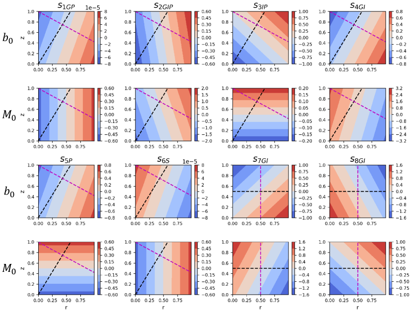
Figure 3: Background states in the simulations, with $b_{0}=b_{r}r+b_{z}z$ and $M_{0}=M_{r}r+M_{z}z$, where the domain-averaged values are subtracted. The black dashed lines indicate the direction parallel to gravity ($\mathbf{e_{R}}$), and the magenta dashed lines indicate the direction perpendicular to gravity ($\mathbf{e_{\theta}}$).

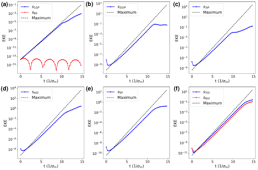
Figure 4: Time series for domain-averaged eddy kinetic energy (EKE), $(u^{\prime 2}+v^{\prime 2}+w^{\prime 2})/2$, in the nonlinear simulations. The blue and red lines show the simulation results, and the black dashed line shows the predicted maximum growth rate of EKE ($2\sigma_{m}$ due to the square). The time is normalized by the maximum growth rate in each simulation (for $s_{6S}$, we use the maximum growth rate for simulation $s_{1GP}$).

For simulations $s_{1GP}$ to $s_{5P}$ and $s_{7GI}$, we begin by initializing them with white noise in the $b^{\prime}$ field. It takes some time for the most unstable mode to grow and become dominant, before which nonlinear effects may already induce turbulence in the system. To emphasize the initial exponential growth phase, we integrate the linearized equations (Equation 14-18 without metric terms) for at least $10/\sigma_{m}$, where $\sigma_{m}$ is the expected maximum growth rate, until the most unstable mode dominates. Subsequently, we use these modes, albeit with reduced amplitude, as initial conditions for nonlinear simulations in each scenario. Only the results of these nonlinear simulations are shown here. In $s_{6S}$, we adopt the same initial conditions as $s_{1GP}$ for the nonlinear simulation, representing stable and unstable scenarios with $Ro\ll 1$. In $s_{8GI}$, we adopt the same initial conditions as $s_{7GI}$ for the nonlinear simulation, because both simulations represent the equatorial plane with identical orientation of the most unstable mode. To ensure numerical stability in the nonlinear simulations, we introduce viscosity ($\nu\nabla^{2}\mathbf{v^{\prime}}$) and diffusivity ($\kappa\nabla^{2}b^{\prime}$) which damp grid-scale noise. The magnitude of the viscosity is chosen such that the viscous term is on the same order as the nonlinear term in the momentum equations for perturbations near the grid-scale. This gives $U^{\prime}\mathcal{M}_{g}\sim\nu U^{\prime}/\Delta^{2}$, where $\mathcal{M}_{g}$ represents the scale of $M_{r}$ or $M_{z}$ (for which we here use the smaller of the prescribed non-zero values of $|M_{r}|$ or $|M_{z}|$ in each simulation), $U^{\prime}$ denotes the scale of the velocity perturbation, and $\Delta$ is the grid scale. Additionally, we set the Prandtl number, $Pr=\nu/\kappa$, to 1, assuming that $\nu$ and $\kappa$ represent sub-grid-scale turbulent transport processes.

3.2 Simulation results

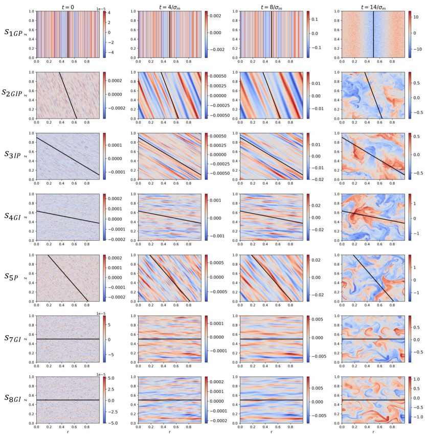
Figure 5: Snapshots of the normalized buoyancy anomaly fields. The buoyancy anomaly is normalized by the maximum value of the background buoyancy field ($b^{\prime}/\mathrm{max}(|b_{0}|)$) in each simulation. The times of the snapshots are indicated above the respective columns and are normalized by the maximum growth rate $\sigma_{m}$ in each simulation. The black solid lines indicate the orientation of the most unstable mode predicted by Equation 35.

For all cases with unstable initial conditions, the simulations reach an approximately exponential growth stage after an initial adjustment period. The growth rates during the exponential growth phase are close to the theoretically predicted maximum growth rates albeit slightly smaller because of the viscous and diffusive dissipation. Eventually, the growth rates reduce significantly because of the onset of nonlinear advection effects (Figure 4).

The simulation with stable background state ($s_{6S}$) does not show exponential growth but an oscillation behaviour. The initial condition used in simulation $s_{6S}$ is the most unstable mode in simulation $s_{1GP}$, which has $k_{z}=0$. In this case, we can estimate the oscillation period $P$ according to the dispersion relation (Equation 28) as $P=584.79$, or 3.14/$\sigma_{m}$ with $\sigma_{m}$ being the maximum growth rate of $s_{1GP}$, consistent with the oscillation period in the simulation (Figure 4a).

During the exponential growth phase of all simulations with an unstable background state, the orientation of the perturbation fields approximately aligns with the most unstable mode predicted by Equation 35, with minor deviations presumably due to the effects of diffusivity and viscosity (Figure 5). The nonlinear simulations are generally quickly dominated by larger modes compared with the modes that dominate the linear simulations (which provide the initial conditions for the nonlinear simulations), because the viscosity and diffusivity are efficient in damping small-scale patterns. At the end of the simulations, nonlinear advection terms are not negligible and the flow becomes turbulent.

The numerical simulations also show that $N^{2}<0$ is neither a sufficient nor necessary condition for instability. In simulation $s_{6S}$, $N^{2}<0$, but the system is stable. In simulations $s_{1GP}$ and $s_{4GI}$, $N^{2}>0$, but the systems are unstable, with either $qf_{0}\sin{\theta}>0$ ($s_{4GI}$) or $qf_{0}\sin{\theta}<0$ ($s_{1GP}$).

In simulations with $Ro\ll 1$ ($s_{1GP}$ and $s_{6S}$), the instability criteria reduce to $b_{z}\sin{\theta}<0$. If the system is unstable, the most unstable mode is parallel to the rotational axis, i.e. slantwise convection parallel to planetary rotation, as shown in simulation $s_{1GP}$.

In the equatorial plane (simulations $s_{7GI}$ and $s_{8GI}$), the growing perturbations are approximately parallel to gravity, despite the fact that in $s_{7GI}$ the instability is caused by zonal wind shear $M_{r}$, while in $s_{8GI}$ the instability is caused by stratification $b_{r}$. This confirms that at the equator, the most unstable mode tends to develop in the upright direction (parallel to gravity), irrespective of whether the instability is caused by stratification or shear.

4 Discussions and conclusions

We find that the necessary and sufficient conditions for instability of zonally symmetric Boussinesq flow on a rotating planet are the background field is (1) gravitationally unstable, or (2) inertially unstable, or (3) the background potential vorticity has a different sign from the planetary vorticity, which is consistent with previous studies on symmetric instability (e.g., Hoskins, 1974). In our framework, we define the gravitational instability criterion as unstable buoyancy stratification along angular momentum surfaces (Equation 40 & Figure 2a) and the inertial instability criterion as unstable angular momentum shear along buoyancy surfaces (Equation 41 & Figure 2b), which ensures both to be sufficient conditions for instability. Mathematically, the criterion for instability can most compactly be expressed as either $b_{z}\sin{\theta}<0$ (i.e. unstable stratification along the planetary rotation axis) or $qf_{0}\sin{\theta}<0$ where $q$ is the potential vorticity (PV). When instability occurs, the growth rate is not sensitive to the magnitude of the radial and vertical wavenumbers, $k_{r}$ and $k_{z}$, but is only a function of their ratio, $k_{r}/k_{z}$, i.e., the tilting direction of the mode.

At the equator, the most unstable mode is always parallel to gravity, irrespective of whether the instability is caused by buoyancy stratification or angular momentum shear.

In the low Rossby number limit, instability occurs if and only if $b_{z}\sin{\theta}<0$, and the most unstable mode is slantwise convection parallel to the planetary rotation axis. The low Rossby number limit proves to be particularly valuable for understanding slantwise convection in icy moon oceans, as this phenomenon is neither properly resolved nor parameterized in global ocean simulations (c.f. Zeng & Jansen, 2024). This limit can also be extended to atmospheric convection on gas giants (e.g., O’Neill & Kaspi, 2016), although this would require a generalization from the Boussinesq approximation to the anelastic approximation (Kaspi et al., 2009).

Unstable stratification in the direction of gravity ($N^{2}<0$), which is excluded a priori in many studies on symmetric instability (e.g., Straneo et al., 2002; Itano & Maruyama, 2009), is found to be neither a necessary nor sufficient condition for symmetric instability. In the low Rossby number limit, such as in icy moon oceans, the onset of slantwise convection depends not on the sign of $N^{2}$ but rather on the stratification parallel to planetary rotation, $b_{z}\sin{\theta}$. This suggests that the traditional convective adjustment scheme widely applied in ocean General Circulation Models (Marotzke, 1991), which parameterizes upright convection when $N^{2}<0$, is not suitable for slantwise convection in icy moon oceans. Although on planets where the fluid layer is shallow and the thin-shell approximation applies, as in Earth’s atmosphere and ocean, the difference between upright and slantwise convection is small, it can become important when the fluid depth is comparable to the planetary radius. Given that $b_{z}\sin{\theta}<0$ is a sufficient condition for symmetric instability, and becomes a sufficient and necessary condition under the low Rossby number limit, we propose that stratification along the rotational axis should be treated as the criterion for static stability and used to trigger convection parameterizations in deep ocean models where the ocean depth is comparable to the planetary radius.

Flasar & Gierasch (1978) and Hathaway et al. (1979) considered cases with $N^{2}<0$ but also assumed that the background flow is in thermal wind balance with no meridional shear, such that $\eta/f=1>0$. Under these assumptions they found that symmetric instability would occur if and only if $qf_{0}\sin{\theta}<0$, consistent with our study (see Appendix B). Our results, however, also show that when the background meridional shear is considered, instability can still occur even when $qf_{0}\sin{\theta}>0$, as demonstrated in Region $S_{4}$ in Figure 2 and simulation $s_{4GI}$, which represents a parameter regime not considered in Flasar & Gierasch (1978) and Hathaway et al. (1979).

Our study focuses exclusively on zonally symmetric instabilities. However, asymmetric modes could also play a significant role in fluid motions on a rotating planet. For instance, equatorial convective rolls driven by heating from the bottom of the fluid are believed to be crucial in driving the equatorial jets on giant planets (e.g., Busse & Hood, 1982; Busse & Or, 1986). Therefore, it is important to characterize the growth rate of different symmetric and asymmetric unstable modes to determine under which regime the symmetric mode dominates. Stone (1966) studied the growth rate of symmetric instabililty, Kelvin-Helmholtz instability, and baroclinic instability on an $f$-plane with hydrostatic balance. He concludes that on an $f$-plane, symmetric instability prevails when $0.25<Ri<0.95$; Kelvin-Helmholtz instability dominates for $Ri<0.25$; and baroclinic instability is dominant when $Ri>0.95$. When considering the horizontal component of planetary rotation, Jeffery & Wingate (2009) suggest that the transition point between symmetric and baroclinic instability dominance can exceed 0.95. Understanding how the symmetric mode, such as slantwise convection in the low Rossby number limit, interacts with baroclinic instability under arbitrary background stratification and shear, and determining the threshold that separates symmetric and asymmetric mode dominance, are important future research directions.

Our studies apply a linear instability analysis method, which is valuable for small-amplitude perturbations but is not applicable to finite-amplitude perturbations or non-linear instability problems. Bowman & Shepherd (1995) applied the energy-Casimir stability method (Holm et al., 1985; Shepherd, 1990; Cho et al., 1993) to study nonlinear symmetric instability where the hydrostatic approximation is made and the rotation is aligned with gravity. However, extending this approach to a more generalized setup (e.g., Fruman & Shepherd, 2008) presents challenges that remain to be addressed in future work. In our current study, we adopt an idealized setup where viscous and diffusive effects are neglected, and solutions are sought on an infinitely large domain (local plane-wave solutions). Future work should also explore the impact of viscosity and diffusivity on instability growth rates, as well as how specific boundary conditions might modify the characteristics of the most unstable modes.

[Acknowledgements]We thank Noboru Nakamura, Wanying Kang, and Hao Fu for helpful discussions and comments.

[Funding]This research received no specific grant from any funding agency, commercial or not-for-profit sectors.

[Declaration of interests]The authors report no conflict of interest.

[Data availability statement]The data that support the findings of this study are openly available in Zenodo at https://doi.org/10.5281/zenodo.14020791.

[Author ORCIDs]Yaoxuan Zeng, https://orcid.org/0000-0002-2624-8579; Malte F. Jansen, https://orcid.org/0000-0002-6479-8651

Appendix A Special case when $b_{r}=0$

In this section, we discuss the special case when $b_{r}=0$. In this case, the dispersion relation (Equation 28) becomes

$$\omega^{2}=\frac{b_{z}\sin{\theta}k_{r}^{2}+f_{0}M_{r}k_{z}^{2}}{k_{r}^{2}+k_{z}^{2}}.$$ (51)

Therefore, the instability criteria reduce to $b_{z}\sin{\theta}<0$ or $f_{0}M_{r}<0$, i.e. the instability for perturbations in the vertical or radial directions. When the system is unstable, the most unstable mode becomes

$$\lim_{b_{r}\to 0}\tan{\delta_{m}}\to\begin{cases}-\frac{b_{r}\sin{\theta}}{b_{z}\sin{\theta}-f_{0}M_{r}-b_{r}\cos{\theta}}\to 0&\mathrm{if}\ b_{z}\sin{\theta}-f_{0}M_{r}>0,\\ \frac{b_{z}\sin{\theta}-f_{0}M_{r}-b_{r}\cos{\theta}}{b_{r}\sin{\theta}}\to\pm\infty&\mathrm{if}\ b_{z}\sin{\theta}-f_{0}M_{r}<0,\end{cases}$$ (52)

with the maximum growth rate being

$$\lim_{b_{r}\sin{\theta}\to 0}\sigma_{m}\to\begin{cases}(-f_{0}M_{r})^{1/2}&\mathrm{if}\ b_{z}\sin{\theta}-f_{0}M_{r}>0,\\ (-b_{z}\sin{\theta})^{1/2}&\mathrm{if}\ b_{z}\sin{\theta}-f_{0}M_{r}<0.\end{cases}$$ (53)

This indicates that the most unstable mode always aligns with either the radial ($\delta_{m}=0$) or vertical ($\delta_{m}=\pi/2$) directions, depending on the magnitude of the growth rate in these two directions, $(-f_{0}M_{r})^{1/2}$ and $(-b_{z}\sin{\theta})^{1/2}$.

Appendix B Instability analysis for $N^{2}<0$ and $\eta/f<0$

In this section, we show that $N^{2}<0$ is not a sufficient condition for instability in a zonally symmetric flow, while $\eta/f<0$ is a sufficient condition for instability.

$N^{2}$ can be expressed as

$$N^{2} = \frac{\partial b_{0}}{\partial R}$$ (54)

$$= b_{z}\sin{\theta}+b_{r}\cos{\theta}$$

$$= |b_{r}\sin{\theta}|\left[\frac{b_{z}\sin{\theta}}{|b_{r}\sin{\theta}|}+\frac{b_{r}}{|b_{r}|}\frac{\cos{\theta}}{|\sin{\theta}|}\right]$$

$$= |b_{r}\sin{\theta}|[x+|\cot{\theta}|\mathrm{sgn}(b_{r})],$$

where $x=b_{z}\sin{\theta}/|b_{r}\sin{\theta}|$ and $y=(f_{0}M_{r}+b_{r}\cos{\theta})/|b_{r}\sin{\theta}|$ are defined in Equation 37, and we used the definition that $\theta\in(-\pi/2,\pi/2]$ so that $\cos{\theta}>0$. Therefore, $N^{2}<0$ is equivalent to

$$x<-|\cot{\theta}|\mathrm{sgn}(b_{r}).$$ (55)

The blue lines mark Equation 55 in Figure 6 when $\theta=60^{\circ}$. As indicated in the plot, when $b_{r}<0$, $N^{2}<0$ is not a sufficient condition for instability as the system can remain stable even when $N^{2}<0$, which is consistent with results shown in the numerical simulation $s_{6S}$.

For comparison with the inertial instability criterion $\eta/f<0$ in previous works such as Itano & Maruyama (2009), we neglect the geometric terms so that $f_{0}=2\Omega$ and $M_{r}=f_{0}+\partial u_{0}/\partial r$. Note that

$$\frac{1}{R}\frac{\partial u_{0}}{\partial\theta}=\frac{\partial u_{0}}{\partial z}\cos{\theta}-\frac{\partial u_{0}}{\partial r}\sin{\theta}=M_{z}\cos{\theta}-(M_{r}-f_{0})\sin{\theta}.$$ (56)

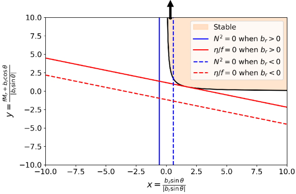
Figure 6: Instability diagram for $\theta=60^{\circ}$ (other latitudes have similar results). Blue lines indicate $N^{2}=0$, and red lines indicate $\eta/f=0$, with solid lines indicating the results for $b_{r}>0$ and dashed lines indicating the results for $b_{r}<0$. The shading indicates the stable region. The black arrow indicates the parameters for simulation $s_{6S}$. Note that for $s_{6S}$, the $y$-axis value is $1.15\times 10^{4}$, outside the $y$-values shown in the plot.

As a result,

$$\frac{\eta}{f} = \frac{f_{0}\sin{\theta}-\frac{1}{R}\frac{\partial u_{0}}{\partial\theta}}{f_{0}\sin{\theta}}$$ (57)

$$= \frac{M_{r}\sin{\theta}-M_{z}\cos{\theta}}{f_{0}\sin{\theta}}$$

$$= \frac{M_{r}\sin{\theta}-\frac{b_{r}\sin{\theta}-b_{z}\cos{\theta}}{f_{0}}\cos{\theta}}{f_{0}\sin{\theta}}$$

$$= \frac{f_{0}M_{r}-b_{r}\cos{\theta}+b_{z}\sin{\theta}\cot^{2}{\theta}}{f_{0}^{2}}$$

$$= \frac{|b_{r}\sin{\theta}|}{f_{0}^{2}}\left[\frac{f_{0}M_{r}+b_{r}\cos{\theta}}{|b_{r}\sin{\theta}|}+\frac{b_{z}\sin{\theta}\cot^{2}{\theta}}{|b_{r}\sin{\theta}|}-\frac{2b_{r}\cos{\theta}}{|b_{r}\sin{\theta}|}\right]$$

$$= \frac{|b_{r}\sin{\theta}|}{f_{0}^{2}}\left[y+\cot^{2}{\theta}x-2|\cot{\theta}|\mathrm{sgn}(b_{r})\right].$$

Therefore, $\eta/f<0$ is equivalent to

$$y<-\cot^{2}{\theta}x+2|\cot{\theta}|\mathrm{sgn}(b_{r}).$$ (58)

The separating line described by Equation 58 is always tangential to the hyperbolic curve, $xy=1$ (see the red line in Figure 6 for the case with $\theta=60^{\circ}$). $\eta/f<0$ is therefore always a sufficient condition for instability.

References

- Bire et al. (2022) Bire, Suyash, Kang, Wanying, Ramadhan, Ali, Campin, Jean-Michel & Marshall, John 2022 Exploring ocean circulation on icy moons heated from below. Journal of Geophysical Research: Planets 127 (3), e2021JE007025.
- Bowman & Shepherd (1995) Bowman, John C & Shepherd, Theodore G 1995 Nonlinear symmetric stability of planetary atmospheres. Journal of Fluid Mechanics 296, 391–407.
- Burns et al. (2020) Burns, Keaton J, Vasil, Geoffrey M, Oishi, Jeffrey S, Lecoanet, Daniel & Brown, Benjamin P 2020 Dedalus: A flexible framework for numerical simulations with spectral methods. Physical Review Research 2 (2), 023068.
- Busse (1970) Busse, F. H. 1970 Thermal instabilities in rapidly rotating systems. Journal of Fluid Mechanics 44 (3), 441–460.
- Busse & Hood (1982) Busse, Friedrich H & Hood, LL 1982 Differential rotation driven by convection in a rapidly rotating annulus. Geophysical & Astrophysical Fluid Dynamics 21 (1-2), 59–74.
- Busse & Or (1986) Busse, Friedrich H & Or, AC 1986 Convection in a rotating cylindrical annulus: thermal rossby waves. Journal of Fluid Mechanics 166, 173–187.
- Callies & Ferrari (2018) Callies, Jörn & Ferrari, Raffaele 2018 Baroclinic Instability in the Presence of Convection. Journal of Physical Oceanography 48 (1), 45–60.
- Cho et al. (1993) Cho, HR, Shepherd, TG & Vladimirov, VA 1993 Application of the direct liapunov method to the problem of symmetric stability in the atmosphere. Journal of the atmospheric sciences 50 (6), 822–836.
- Christensen (2002) Christensen, Ulrich R 2002 Zonal flow driven by strongly supercritical convection in rotating spherical shells. Journal of Fluid Mechanics 470, 115–133.
- Eliassen (1951) Eliassen, Arnt 1951 Slow thermally or frictionally controlled meridional circulation in a circular vortex. Astrophisica Norvegica, v. 5, p. 19 5, 19.
- Emanuel (1983) Emanuel, Kerry A 1983 The lagrangian parcel dynamics of moist symmetric instability. Journal of Atmospheric Sciences 40 (10), 2368–2376.
- Emanuel (1985) Emanuel, Kerry A 1985 Convective adjustment in baroclinic atmospheres. The Jovian Atmospheres 2441, 163–171.
- Flasar & Gierasch (1978) Flasar, F. Michael & Gierasch, Peter J. 1978 Turbulent convection within rapidly rotating superadiabatic fluids with horizontal temperature gradients. Geophysical & Astrophysical Fluid Dynamics 10 (1), 175–212.
- Fruman & Shepherd (2008) Fruman, Mark D. & Shepherd, Theodore G. 2008 Symmetric Stability of Compressible Zonal Flows on a Generalized Equatorial Plane. Journal of the Atmospheric Sciences 65 (6), 1927–1940.
- Galanti et al. (2019) Galanti, Eli, Kaspi, Yohai, Miguel, Yamila, Guillot, Tristan, Durante, Daniele, Racioppa, Paolo & Iess, Luciano 2019 Saturn’s deep atmospheric flows revealed by the cassini grand finale gravity measurements. Geophysical Research Letters 46 (2), 616–624.
- Haine & Marshall (1998) Haine, Thomas W. N. & Marshall, John 1998 Gravitational, Symmetric, and Baroclinic Instability of the Ocean Mixed Layer. Journal of Physical Oceanography 28 (4), 634–658.
- Hathaway et al. (1979) Hathaway, David H., Gilman, Peter A. & Toomre, Juri 1979 Convective instability when the temperature gradient and rotation vector are oblique to gravity. I. Fluids without diffusion. Geophysical & Astrophysical Fluid Dynamics 13 (1), 289–316.
- Heimpel et al. (2016) Heimpel, Moritz, Gastine, Thomas & Wicht, Johannes 2016 Simulation of deep-seated zonal jets and shallow vortices in gas giant atmospheres. Nature Geoscience 9 (1), 19–23.
- Holm et al. (1985) Holm, Darryl D, Marsden, Jerrold E, Ratiu, Tudor & Weinstein, Alan 1985 Nonlinear stability of fluid and plasma equilibria. Physics reports 123 (1-2), 1–116.
- Hoskins (1974) Hoskins, B. J. 1974 The role of potential vorticity in symmetric stability and instability. Quarterly Journal of the Royal Meteorological Society 100 (425), 480–482.
- Itano & Maruyama (2009) Itano, Toshihisa & Maruyama, Kiyoshi 2009 Symmetric Stability of Zonal Flow under Full-Component Coriolis Force -Effect of the Horizontal Component of the Planetary Vorticity-. Journal of the Meteorological Society of Japan. Ser. II 87 (4), 747–753.
- Jansen et al. (2023) Jansen, Malte F, Kang, Wanying, Kite, Edwin S & Zeng, Yaoxuan 2023 Energetic constraints on ocean circulations of icy ocean worlds. The Planetary Science Journal 4 (6), 117.
- Jeffery & Wingate (2009) Jeffery, Nicole & Wingate, Beth 2009 The Effect of Tilted Rotation on Shear Instabilities at Low Stratifications. Journal of Physical Oceanography 39 (12), 3147–3161.
- Kang et al. (2022) Kang, Wanying, Mittal, Tushar, Bire, Suyash, Campin, Jean-Michel & Marshall, John 2022 How does salinity shape ocean circulation and ice geometry on enceladus and other icy satellites? Science advances 8 (29), eabm4665.
- Kaspi et al. (2009) Kaspi, Yohai, Flierl, Glenn R & Showman, Adam P 2009 The deep wind structure of the giant planets: Results from an anelastic general circulation model. Icarus 202 (2), 525–542.
- Kaspi et al. (2023) Kaspi, Yohai, Galanti, Eli, Park, RS, Duer, K, Gavriel, N, Durante, D, Iess, L, Parisi, M, Buccino, DR, Guillot, T & others 2023 Observational evidence for cylindrically oriented zonal flows on jupiter. Nature Astronomy 7 (12), 1463–1472.
- Kaspi et al. (2018) Kaspi, Y ea, Galanti, E, Hubbard, William B, Stevenson, DJ, Bolton, SJ, Iess, L, Guillot, T, Bloxham, J, Connerney, JEP, Cao, H & others 2018 Jupiter’s atmospheric jet streams extend thousands of kilometres deep. Nature 555 (7695), 223–226.
- Marotzke (1991) Marotzke, Jochem 1991 Influence of convective adjustment on the stability of the thermohaline circulation. Journal of Physical Oceanography 21 (6), 903–907.
- O’Neill & Kaspi (2016) O’Neill, Morgan E & Kaspi, Yohai 2016 Slantwise convection on fluid planets. Geophysical Research Letters 43 (20).
- Ooyama (1966) Ooyama, Katsuyuki 1966 On the stability of the baroclinic circular vortex: A sufficient criterion for instability. Journal of Atmospheric Sciences 23 (1), 43–53.
- Shepherd (1990) Shepherd, Theodore G 1990 Symmetries, conservation laws, and hamiltonian structure in geophysical fluid dynamics. In Advances in Geophysics, , vol. 32, pp. 287–338. Elsevier.
- Soderlund (2019) Soderlund, Krista M 2019 Ocean dynamics of outer solar system satellites. Geophysical Research Letters 46 (15), 8700–8710.
- Stevens (1983) Stevens, Duane E 1983 On symmetric stability and instability of zonal mean flows near the equator. Journal of the Atmospheric Sciences 40 (4), 882–893.
- Stone (1966) Stone, Peter H 1966 On non-geostrophic baroclinic stability. Journal of the Atmospheric Sciences 23 (4), 390–400.
- Stone (1967) Stone, Peter H 1967 An application of baroclinic stability theory to the dynamics of the jovian atmosphere. Journal of Atmospheric Sciences 24 (6), 642–652.
- Stone (1971) Stone, Peter H. 1971 The symmetric baroclinic instability of an equatorial current. Geophysical Fluid Dynamics 2 (1), 147–164.
- Straneo et al. (2002) Straneo, Fiammetta, Kawase, Mitsuhiro & Riser, Stephen C. 2002 Idealized Models of Slantwise Convection in a Baroclinic Flow. Journal of Physical Oceanography 32 (2), 558–572.
- Sun (1995) Sun, Wen‐Yih 1995 Unsymmetrical symmetric instability. Quarterly Journal of the Royal Meteorological Society 121 (522), 419–431.
- Vallis (2017) Vallis, Geoffrey K 2017 Atmospheric and oceanic fluid dynamics. Cambridge University Press.
- Walton (1975) Walton, I. C. 1975 The viscous nonlinear symmetric baroclinic instability of a zonal shear flow. Journal of Fluid Mechanics 68 (4), 757–768.
- Zeng & Jansen (2024) Zeng, Yaoxuan & Jansen, Malte F 2024 The effect of salinity on ocean circulation and ice–ocean interaction on enceladus. The Planetary Science Journal 5 (1), 13.