Comments on firewalls in JT gravity with matter

Abstract

We present two discussions of firewalls in JT gravity. First we present an alternative, arguably simpler, derivation of the gray hole conjecture, applying uniformly to all probes of the firewall probability previously discussed. This derivation is based on the wormhole shortening picture using the handle-disk geometry. However we modifies Saad’s story utilizing a ”Wilsonian” effective gravitational description, adapted to the time scale probed, in which high frequency modes are integrated out generating the gravitational bulk geometries (dual to the genus expansion in the matrix integral side) whereas low frequency modes are more precisely resolved by being represented as eigenvalue D-branes where JT universes can end. This treatment results in an effective ”twist factor cutoff” prescription which simplifies the discussion of long time quantities including the firewall probability. In the second part we discuss effects of matter loops on the firewall probability – while naively such effects lead to new divergences, we argue that those correspond to the necessary modification of quantum field theory renormalization in topologically non-trivial spacetimes, and their effect on the firewall probability is small.

1 Introduction and summary

The black hole information paradox is one of the sharp questions in understanding quantum gravity Hawking:1975vcx ; Hawking:1976ra . The discovery of BFSS conjecture Banks:1996vh and AdS/CFT duality Maldacena:1997re ; Gubser:1998bc ; Witten:1998qj suggests that information is not lost, as the dual quantum mechanical systems are inherently unitary. However, AMPS has argued that Almheiri:2012rt ; Almheiri:2013hfa , the entanglement between old Hawking particles and the vacuum degrees of freedom near the horizon would violate monogamy of entanglement, and thus unitarity and monogamy of entanglement leads to a dangerous firewall behind horizon. In recent years, significant progress have been made in addressing the firewall paradox Bousso:2012as ; Nomura:2012sw ; Maldacena:2013xja ; VanRaamsdonk:2013sza ; Almheiri:2014lwa ; Dong:2016eik ; Almheiri:2019hni ; Penington:2019kki ; Almheiri:2019qdq ; Almheiri:2019psf ; Penington:2019npb . Especially, the proposal of ”ER=EPR” Maldacena:2013xja ; Susskind:2014yaa argues that spacetime wormholes formed by entanglement could resolve the apparent violation of entanglement monogamy.

Furthermore, Maldacena suggested a version of the information paradox in the eternal black hole in AdS – the decay in the two-point function at very late times is in tension with the expected discrete spectrum of black hole microstates Maldacena:2001kr . Recent progress also revealed the deep connections between black hole and discrete chaotic quantum systems Shenker:2013pqa ; Cotler:2016fpe ; Saad:2019lba ; Penington:2019kki . In particular, the two-point function in chaotic quantum systems oscillates heavily at late time and the average over these fluctuations exhibits ”ramp-plateau” structure. On the gravity side, the ramp is understood as a signature of spacetime wormholes Saad:2018bqo ; Saad:2019pqd ; Blommaert:2019hjr ; Yan:2022nod .

Recently, Stanford and Yang Stanford:2022fdt examined whether these late time spacetime wormholes could give rise to firewalls and connected this phenomenon to a conjecture made by Susskind Susskind:2015toa . The ”gray hole” conjecture postulates that the typical late time state has equal probability to be in a black hole or white hole state. The initial state prepared by a Euclidean path integral is far from a complexity equilibrium but under an exponentially long Lorentzian time evolution the state is expected to eventually evolves into a typical state and reach a complexity equilibrium. The ensemble of late-time typical states should be time-reversal symmetric, which means that the evolved state should have equal probability to be a black hole state or a white hole state. This gray hole conjecture is related to firewalls in the sense that for an in-falling observer, black holes are considered safe due to their expanding interior, which dilutes perturbations, and white holes are dangerous due to their contracting interior, which enhances perturbations. A precise example was given in Stanford:2022fdt by applying external perturbations to the thermal field double state.

The main tool used in Stanford:2022fdt to investigate the nature of the late time state and its geometry, and thus the gray hole conjecture, is the ”wormhole shortening” mechanism proposed by Saad in Saad:2019pqd . The handle-disk geometry in JT gravity allows a spatial slice of two-sided black hole to emit a baby universe and thus effectively return to its earlier state. Stanford and Yang utilized this mechanism to include sufficiently large baby universes, showing that an old black hole has a nonzero probability to tunnel into a white hole, and that the probability increases to 1/2 at Heisenberg time, consistent with the gray hole conjecture. However, the result raises several questions:

• The white hole probability fails to saturate to 1/2 after Heisenberg time.

• It is difficult to preserve the normalization condition that the sum of black hole and white hole probabilities is unity.

• It is difficult to generalize the result to other circumstances, for example for a single member of the ensemble dual to JT gravity, or including dynamical matter.

The answer to the first two questions is related to non-perturbative effects. Indeed, in Blommaert:2024ftn , the authors calculated the white hole probability by directly using non-perturbative results from the matrix integral dual to JT gravity. They showed that the probabilities indeed saturate to 1/2 after Heisenberg time and that the probabilities sum up to unity at all times. Similarly, non-perturbative operator constructions also imply a finite tunneling probability Iliesiu:2024cnh ; Miyaji:2024ity . These approaches use other probes of the late time state, e.g. the two-point function in Blommaert:2024ftn . However, these non-perturbative approaches obscure somewhat the intuitive and geometrical wormhole shorting picture.

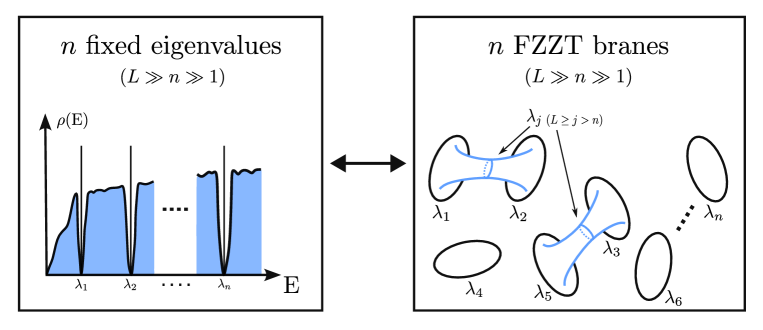
In this paper, we introduce a convenient way to geometrically encode non-perturbative corrections into the wormhole picture. Specifically, starting with a single member of the ensemble, which we refer to as the UV theory, which is discrete and non-geometrical, we perform the ensemble average in stages, in the spirit of a Wilsonian effective description. The effective description suitable for long time quantities keeps the average energy fixed and organizes modes into ”fast” or ”slow” by their energy differences (conjugate to Lorentzian time). By integrating out high frequency ”fast” modes, in this context all of the eigenvalues of the matrix outside of a fixed microcanonical window, we obtain an effective gravitational description consisting of JT gravity with its usual geometric genus expansions, together with additional FZZT D-branes representing the eigenvalues in the fixed microcanonical window, which are the ”slow modes” responsible for the non-perturbative long time effects. This hybrid description retains many of the advantages of the dual geometrical picture, for example the ability to ask inherently geometrical questions, while being adapted to late time quantities.

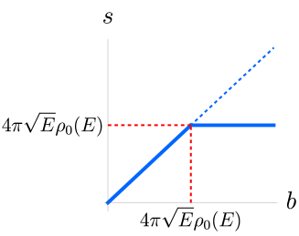
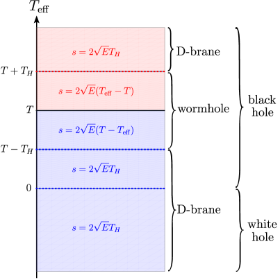
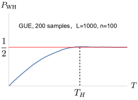
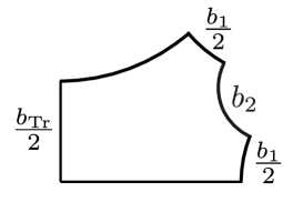
We show then that the effect of singling out the slow modes for a more precise treatment is summarized by a simple modification of the genus expansion in JT gravity. Namely, the twist factor appearing in the sum over Riemann surfaces is replaced by an ”effective twist factor”, most significantly having a cutoff arising from treating the FZZT branes exactly. Incorporating this modification into the wormhole shortening picture, this means that small baby universes will continue to form wormholes with the usual twist factor that scales with size of baby universe. But for large baby universes, they will necessarily end on a configuration of D-branes. In that case, the twist factor cutoff accounts for non-perturbative effects and no longer scales with the size of baby universes. We sketch this cutoff in Fig.1.

Figure 1: Twist factor cutoff: s is the twist factor and b is the size of baby universe.

Using the twist factor cutoff prescription to encode non-perturbative effects, we repeat the calculation of wormhole shortening and its effect on the gray hole conjecture. For concreteness we use the two-point function in JT gravity as a probe. This leads to several important differences between our calculation and Stanford:2022fdt . First, the bulk moduli of the two-point function are unconstrained by mapping class group. Secondly, as we discuss below the Euclidean handle-disk geometry contribution to the two-point function is time-symmetric after analytic continuation to Lorentzian times. This means that at late time the black hole can not only emit a baby universe but also absorb one. As a result, the effective time of an old black hole can be reduced or increased. Thirdly, due to twist factor cut off, large baby universes are emitted to or absorbed from a D-brane. By carefully including both D-brane and wormhole contributions in a time reversal symmetric manner, we obtain the full non-perturbative result that matches with Blommaert:2024ftn :

$$\textbf{For }\mathbf{T<T_{H}}:\quad\mathcal{P}_{\mathrm{BH}}(T)=1-\frac{T}{T_{H}}+\frac{T^{2}}{2T_{H}^{2}},\quad\mathcal{P}_{\mathrm{WH}}(T)=\frac{T}{T_{H}}-\frac{T^{2}}{2T_{H}^{2}};$$

$$\textbf{For }\mathbf{T\geq T_{H}}:\quad\mathcal{P}_{\mathrm{BH}}(T)=\frac{1}{2},\quad\mathcal{P}_{\mathrm{WH}}(T)=\frac{1}{2};$$ (1)

where $\mathcal{P}_{\mathrm{BH}}$ is the probabilities for the late time slice being a black hole state and $\mathcal{P}_{\mathrm{WH}}$ is the probability of being a white hole state, and $\mathrm{T}_{\mathrm{H}}$ is the Heisenberg time.

Thus, the first two questions mentioned above are answered as:

• Saturation of 1/2: After the Heisenberg time, in order to tunnel into white hole all the emitted baby universes necessarily end on D-brane, instead of being traded. This transition leads to saturation of the white hole probability at 1/2.

• Normalization of probability: Treating the Euclidean handle-disk geometry in time reversal symmetric way and properly accounting for baby universes ending on D-brane ensures the total probability sums up to unity.

The effective geometrical picture we use allows us to discuss some generalizations to pure JT gravity. Suppose for example that instead of integrating over the slow degrees of freedom represented as FZZT branes, we keep those eigenvalues fixed. Similar to the spectral form factor, we see that the twist factor heavily fluctuates (as function of the size of baby universe b). Perhaps these heavy fluctuations could be related to a breakdown of the geometric description or strong back-reaction visible to an infalling observer. However, we find that since the black (or white) hole probability is an integral over twist factor, the result becomes self-averaging. Indeed, we can go all the way back to the UV picture, namely a a single member of the ensemble, and find that even in that limit the black (white) hole probability is self-averaging. We therefore conclude

• Individual quantum system: The gray hole conjecture holds for a single quantum system, provided that the system has a sufficiently large number of degrees of freedom and represents a typical draw from the ensemble that reproduces JT gravity. The black (or white) hole probability is self-averaging.

Finally, in the last section we analyze another generalization of pure JT gravity using our effective geometrical description. Namely, we look at the potential source of a firewall arising from matter loops in the handle-disk geometry, as originally suggested in Blommaert:2024ftn . We argue that this matter loop effect is benign, being essentially the same as what occurs in the vacuum state near the black hole horizon. Indeed, the naive divergence of matter loops in the geometry corresponds to necessary modification of quantum field theory renormalization in topologically non-trivial spacetime, rather than a physical firewall. We estimate the effective contribution of matter loops by directly placing the matter loops on the dominant geometry that contributes to the two-point function and show that their contributions are small.

This paper is structured as follows. In Sec.2, we review JT gravity and Saad’s wormhole shortening picture. In Sec.3, we construct the effective description of a microcanonical window involving JT gravity accompanied by FZZT branes and calculate the cutoff on the effective twist factor. In Sec.4, we use the twist factor cutoff to calculate the probabilities of effective time slice using handle-disk geometry and make some comments on the results. In Sec.5, we examine the effect of matter in the wormhole background and argue that the matter loop correction does not lead to a firewall.

2 Wormhole shortening in JT gravity

In this section we briefly review JT gravity, mainly for the purpose of explaining our notations and conventions. For more details we refer interested reader to overviews in e.g. Sarosi:2017ykf ; Trunin:2020vwy ; Mertens:2022irh ; Jafferis:2022wez . We then summarize Saad’s perspective on the ”wormhole shortening” effect in the handle-disk geometry Saad:2019lba which corresponds to the process of baby universe exchange. In the following section we argue that this picture is modified for sufficiently large baby universes and present a more complete picture.

2.1 JT gravity setup

JT gravity is a 2d dilaton gravity model with a special choice of linear dilaton potential:

$$I_{\mathrm{JT}}=-\frac{S_{0}}{2\pi}\left[\frac{1}{2}\int_{\mathcal{M}}\sqrt{g}R+\int_{\partial\mathcal{M}}\sqrt{h}K\right]-\left[\frac{1}{2}\int_{\mathcal{M}}\sqrt{g}\phi(R+2)+\int_{\partial\mathcal{M}}\sqrt{h}\phi(K-1)\right],$$ (2)

where $\mathcal{M}$ is a two-dimensional manifold with Euclidean metric $g$, $h$ is pull-back metric at the boundary $\partial\mathcal{M}$, $S_{0}$ is the extremal entropy (appearing as a free parameter in JT) and $\phi$ denotes the dilaton field. The first bracket is a topological invariant proportional to the Euler characteristic: $-S_{0}\mathcal{X}$, and the dynamics comes from the second bracket.

Below we will be interested in boundaries in JT gravity. There are in total four inequivalent boundary conditions Goel:2020yxl . For now we will mostly be interested in the Dirichlet-Dirichlet (DD) boundary condition, which corresponding to asymptotically $AdS$ boundaries, such that the regulated boundary length is fixed to be $\frac{\beta}{\epsilon}$ and the dilaton value at boundary is $\frac{1}{2\epsilon}$. When discussing D-branes below, We will also consider Dirichlet-Neumann (DN) and Neumann-Dirichlet (ND) boundary conditions studied in Goel:2020yxl .

After integrating out dilaton field, the bulk of JT gravity is frozen to be locally $\mathrm{AdS}_{2}$ and the only dynamics comes from boundary gravitons, which can be described as a one-dimensional Schwarzian theory with a density of states at disk level Cotler:2016fpe ; Stanford:2017thb ; Yang:2018gdb :

$$\rho_{0}(E)=\frac{e^{S_{0}}}{2\pi^{2}}\sinh{\left(2\pi\sqrt{E}\right)}.$$ (3)

The two-sided Hilbert space (dual to the eternal black hole) can be described in different bases, related by different resolution of the identity operator Yang:2018gdb ; Saad:2019pqd :

$$\mathds{1} =\int_{0}^{\infty}dE\rho_{0}(E)|E\rangle\langle E|=e^{-S_{0}}\int_{-\infty}^{\infty}d\ell|\ell\rangle\langle\ell|,$$ (4)

where $|E\rangle$ is the energy basis, $|\ell\rangle$ is the length basis with renormalized length $\ell$ of a spatial slice. These bases obey the orthogonality relations:

$$e^{-S_{0}}\int_{-\infty}^{\infty}d\ell\langle E|\ell\rangle\langle\ell|E^{\prime}\rangle =\frac{\delta(E-E^{\prime})}{\rho_{0}(E)},$$ (5)

$$\int_{0}^{\infty}dE\rho_{0}(E)\langle\ell|E\rangle\langle E|\ell^{\prime}\rangle =e^{S_{0}}\delta(\ell-\ell^{\prime}),$$ (6)

The Wheeler-Dewitt wavefunction $\langle\ell|E\rangle$ is given as Harlow:2018tqv ; Yang:2018gdb :

$$\psi_{E}(\ell)\equiv\langle\ell|E\rangle=2K_{2i\sqrt{E}}(2e^{-\ell/2}).$$ (7)

One can then express bulk Hartle-Hawking state $|HH_{\beta/2}\rangle$ with boundary length $\beta/2$ in terms of energy basis:

$$|HH_{\beta/2}\rangle=\int_{0}^{\infty}dE\,\rho_{0}(E)\,e^{-\frac{\beta}{2}E}|E\rangle.$$ (8)

By using (7), the Hartle-Hawking state can also be expressed in the length basis. The disk partition function of JT gravity can be interpreted as the inner product of two Hartle-Hawking states Saad:2019pqd :

$$Z_{\mathrm{disk}}(\beta)=\langle HH_{\beta/2}|HH_{\beta/2}\rangle=\frac{e^{S_{0}}}{2\sqrt{\pi}\beta^{\frac{3}{2}}}e^{\frac{\pi^{2}}{\beta}}.$$ (9)

More generally, higher topologies with multiple asymptotic boundaries can be obtained from surfaces with geodesic boundaries by gluing a trumpet geometry, which has an asymptotic boundary of length $\beta$ and a geodesic boundary of length $b$, for each such boundary Saad:2019lba . The moduli space of surfaces of fixed geodesic boundaries is given by Weil-Petersson volume $V_{g,n}(b_{1},...,b_{n})$, then partition function for genus g surfaces with asymptotic boundaries is given by,

$$Z_{g,n}(\beta_{1},...,\beta_{n})=\int_{0}^{\infty}b_{1}db_{1}...\int_{0}^{\infty}b_{n}db_{n}V_{g,n}(b_{1},...,b_{n})\psi_{\mathrm{Tr}}(\beta_{1},b_{1})...\psi_{\mathrm{Tr}}(\beta_{n},b_{n}),$$ (10)

where the trumpet contribution is denoted as $\psi_{\mathrm{Tr}}(\beta,b)$, $n$ is the number of asymptotic boundaries and $g$ is the genus. The measure factors $b_{i}$ are included due to possible twists in the gluing process and they become very important for the late time behavior of many quantities, as we discuss further below.

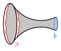
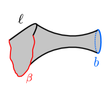
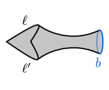
Another perspective on the above description is to treat the addition of a geodesic boundary $b$ as an adding a closed baby universe state, interpreted in a third quantized language. The above trumpet geometry can then be expressed as the following wavefunction in the third quantized Hilbert space Yang:2018gdb ; Saad:2019pqd :

$$\psi_{\mathrm{Tr}}(\beta,b) \equiv\langle HH_{\beta/2}|b,HH_{\beta/2}\rangle=\int dE\frac{\cos(b\sqrt{E})}{2\pi\sqrt{E}}e^{-\beta E}.$$ (11)

By inserting the resolutions of the identity in (5) and (6) into the above expression, one can also obtain the following trumpet wave functions:

$$\psi_{\mathrm{Tr},\beta/2}(\ell,b) \equiv\langle HH_{\beta/2}|\ell,b\rangle=\int_{0}^{\infty}dE\frac{\cos(b\sqrt{E})}{2\pi\sqrt{E}}e^{-\frac{\beta}{2}E}\psi_{E}(\ell),$$ (12)

$$\langle\ell^{\prime}|\ell,b\rangle =\int_{0}^{\infty}dE\frac{\cos(b\sqrt{E})}{2\pi\sqrt{E}}\psi_{E}(\ell)\psi_{E}(\ell^{\prime}).$$ (13)

We draw the geometric pictures of above three kinds of trumpet wave functions in Fig.2.

Figure 2: (a) asymptotic boundary $\beta$ with geodesic boundary $b$: $\psi_{\mathrm{Tr}}(\beta,b)$; (b) mixed asymptotic boundaries $\beta,\ell$ with geodesic boundary $b$: $\psi_{\mathrm{Tr},\beta/2}(\ell,b)$; (c) asymptotic boundaries $\ell,\ell^{\prime}$ with geodesic boundary b: $\langle\ell^{\prime}|\ell,b\rangle$

2.2 Including matter

We will also consider JT gravity minimally coupling to a free massive scalar field by adding the following action:

$$I_{m}=\frac{1}{2}\int_{\mathcal{M}}\sqrt{g}\left(g^{ab}\partial_{a}\chi\partial_{b}\chi+m^{2}\chi^{2}\right),$$ (14)

where the matter field $\chi$ couples to the metric but not to the dilaton. We take the Dirichlet boundary condition so that the dual boundary operator $\mathcal{O}$ has scaling dimension:

$$\Delta=\frac{1}{2}+\sqrt{\frac{1}{4}+m^{2}}.$$ (15)

We are interested in the Lorentzian correlator of two-sided boundary operators in the probe limit, meaning that back-reaction effects are ignored. This two-point function at Lorentzian time T is defined as:

$$G_{\Delta}(T)\equiv\frac{1}{Z(\beta)}\langle HH_{\beta/2}|e^{iHT}\mathcal{O}_{L}\mathcal{O}_{R}e^{-iHT}|HH_{\beta/2}\rangle.$$ (16)

where we use in the definition the bulk Hartle-Hawking state creating the two sided black hole at $T=0$ and bulk two-sided Hamiltonian $H_{L}+H_{R}$ which propagates both left and right boundary operators in time (the combination $H_{L}-H_{R}$ is a symmetry).

At the disk level, the boundary propagator is Yang:2018gdb :

$$\langle\mathcal{O}(x_{1})\mathcal{O}(x_{2})\rangle_{\mathrm{disk}}=e^{-\Delta\ell(x_{1},x_{2})},$$ (17)

where $\ell(x_{1},x_{2})$ is the renormalized length of the bulk geodesic connecting the boundary locations $x_{1}$ and $x_{2}$. Thus the two-point function on the disk geometry can be easily calculated by inserting an identity operator expressed in the length basis, which yields:

$$G_{\Delta}^{\mathrm{disk}}(T)=\frac{e^{-S_{0}}}{Z(\beta)}\int_{-\infty}^{\infty}d\ell\langle HH_{\beta/2+iT}|\ell\rangle\langle\ell|HH_{\beta/2-iT}\rangle e^{-\Delta\ell}.$$ (18)

We present this formula geometrically as below:

$$G_{\Delta}^{\mathrm{disk}}(T) =\leavevmode\hbox{$\vbox{\hbox{\resizebox{}{}{{\leavevmode\hbox{\set@color{}}}}}}$},$$ (19)

$$=\frac{e^{-S_{0}}}{Z(\beta)}\int_{-\infty}^{\infty}d\ell\leavevmode\hbox{$\vbox{\hbox{\resizebox{}{}{{\leavevmode\hbox{\set@color{}}}}}}$}e^{-\Delta\ell}$$ (20)

Two-point function on higher genus geometries requires summing over all inequivalent geodesics in the bulk. We will calculate the genus one case in detail in Sec.4.

2.3 Wormhole shortening

In Saad:2019pqd , Saad established a nice ”wormhole shortening” picture for understanding the ramp structure in the spectral form factor (SFF) and two-point functions at late time (in the next section we further discuss the structure of the plateau). Here we review the picture in the context of the SFF, for full details we refer to the original paper Saad:2019pqd .

The SFF can be reformulated as the ”return probability”:

$$|Z(\beta+iT)|^{2}=|\langle HH_{\beta/2}|e^{-iTH}|HH_{\beta/2}\rangle|^{2}.$$ (21)

This is the probability for the Hartle-Hawking state to return to itself after a Lorentzian evolution of time T. The states in JT gravity can be characterized by the length of the Einstein-Rosen bridge (ERB). Therefore, the magnitude of the SFF quantifies the probability for the length of ERB at late time to go back to its initial value.

The leading order contributions to the SFF at early time are two disconnected disks. The size of the ERB of at Lorentzian time $T$ can be obtained by calculating the expectation value of the length operator $\ell$ in the Hartle-Hawking state. The semi-classical result shows that ERB grows linearly at late times Yang:2018gdb :

$$\mathcal{V}(t)=\frac{e^{-S_{0}}}{Z(\beta)}\int_{-\infty}^{\infty}d\ell\langle HH_{\beta/2+iT}|\ell\rangle\langle\ell|HH_{\beta/2+iT}\rangle\ell\approx\frac{2\pi T}{\beta},\quad T\gg\beta,$$ (22)

where $\beta$ has being analytically continued to $\beta+iT$ to account for the Lorentzian evolution of the Hartle-Hawking state: $|HH_{\beta/2+iT}\rangle=e^{-iTH}|HH_{\beta/2}\rangle$. Since the length of the ERB is growing linearly with respect to Lorentzian time, the return amplitude decreases, giving the early time ”slope”. We illustrate the Lorentzian picture for the disk topology in Fig.3.

Figure 3: Disk contribution to the SFF. Red and blue lines represent the ERB, with their length qualitatively corresponding to ERB length.

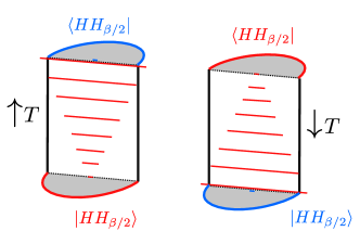
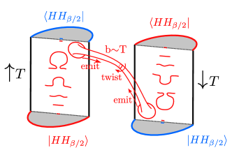
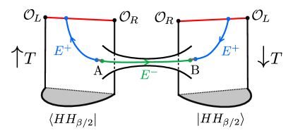
At late enough time when the disk contribution decays to be sufficiently small, the next order topology, the handle-disk, dominates the SFF. This topology allows the two systems to exchange a baby universe with arbitrary size, meaning that the length of ERB can be reduced or enlarged by emitting or absorbing a baby universe. It turns out that the length is approximately conserved in this process, $\ell\sim\ell_{T}\pm b$, where $b$ is the size of baby universe and $\ell_{T}$, $\ell$ represent the sizes of the ERB before and after the exchange process, and $\pm$ signs stands for the possibility of emitting/absorbing a baby universe. We see then that if the size of an emitted baby universe is approximately $b\sim T$, the baby universe exchange reduces the length of ERB to its original length at $T=0$ and thus provides a non-decaying amplitude.

Importantly, the exchange process involves gluing of two-baby universes emitted from both copies of the system with an arbitrary twist. This twist measure factor is responsible for the appearance of a linear in $T$ ramp. This mechanism is also responsible for the appearance of a ramp of two-point function (and higher correlation functions) at late times Saad:2019pqd .

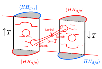
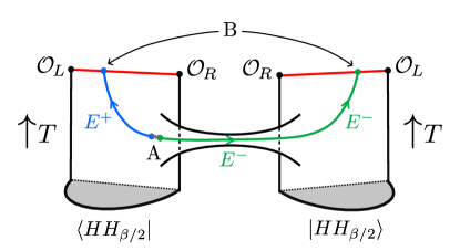
We note that since the baby universe exchange originates from a Euclidean geometry, such process must be time-reversal symmetric in the Lorentzian picture. This means the baby universe can be emitted or absorbed with equal probability. However, since the absorbing process further increases the ERB length, it is always sub-dominant in the SFF (and two-point functions). Nevertheless, keeping a time-reversal symmetric treatment by including the absorption process is essential for the proper normalization of the total probability, a point we will come back to in Sec.4. We illustrate both emission and absorption process in the Lorentzian signature in Fig. 4.

Figure 4: (a) Emitting process: The length of ERB is shortened by the emission of a baby universe with size T, resulting a non-decaying return amplitude. The twist factor gives linear ramp. (b) Absorbing process: The ERB length is enlarged through the absorption of a baby universe, which further decreases the return amplitude. Absorption process provides sub-dominant contribution to SFF.

The above picture accounts for the ramp at times earlier than the Heisenberg time and receives only small corrections in the genus expansion. In the next section we extend this geometrical picture to later time, we will see that this results in a similar geometrical picture with an effective cutoff on the twist factor for large baby universes.

3 FZZT-branes and twist factor cutoff

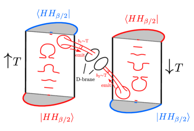
After the Heisenberg time non-perturbative effects dominate the SFF. In Saad:2019pqd it was suggested that this regime could be described by including D-brane boundaries, such that emitted baby universes end on D-branes instead of being exchanged. This geometrical picture eliminates the twist factor measure, resulting in a plateau in the SFF. The Lorentzian picture is illustrated in Fig.5. In this section we substantiate this geometrical picture using FZZT or eigen-branes, and in the next section we then apply it to the calculation of the firewall probability at late times and the gray hole conjecture.

Figure 5: D-brane picture for plateau.

3.1 FZZT branes

JT gravity is dual to a double scaled matrix integral Saad:2019lba , i.e. the topological expansion of JT gravity (10) can be computed by the ensemble average of the matrix operators $\mathrm{Tr}e^{\beta_{i}M}$:

$$\langle Z(\beta_{1})...Z(\beta_{n})\rangle_{\mathrm{JT}} =\sum_{g=0}^{\infty}e^{S_{0}(2-2g-n)}Z_{g,n}(\beta_{1},...,\beta_{n}),$$ (23)

$$=\frac{1}{Z_{L}}\int\mathcal{D}H\,e^{-L\,\mathrm{Tr}V(H)}\,\mathrm{Tr}\,e^{\beta_{i}H}...\,\mathrm{Tr}\,e^{\beta_{n}H},$$ (24)

where H is $L\times L$ ($L\gg 1$) Hermitian matrix with potential $V(H)$ and $Z_{L}$ is partition function for this matrix ensemble: $Z_{L}=\int\mathcal{D}He^{-L\,\mathrm{Tr}V(H)}$.

As is common in the matrix/gravity correspondence, each eigenvalue of the matrix corresponds to a D-brane. On the gravity side, fixing an eigenvalue can be realized by insertion of a D-brane boundary with fixed energy and dilaton value Blommaert:2019wfy , that is the DN boundary condition discussed in Goel:2020yxl . In minimal string theory these corresponds to FZZT branes, and we use that term in our context as well. In the dual matrix integral a boundary with fixed energy $\lambda$ corresponds to an operator insertion:

$$\mathcal{O}(\lambda)=-\int_{0}^{\infty}\frac{d\beta}{\beta}e^{\beta\lambda}Z(\beta)=\mathrm{Tr}\log(\lambda-H)-\frac{L}{2}V(\lambda),$$ (25)

where $\frac{1}{\beta}$ means we consider an unmarked boundary and divide the gauge group volume $\mathrm{Vol}(S^{1})=\beta$. Then the FZZT brane operator is the exponential, corresponding to an insertion of any number of boundaries:

$$\psi(\lambda)=\exp\left(\mathcal{O}(\lambda)\right)=\det(\lambda-H)\exp\left(-\frac{L}{2}V(\lambda)\right).$$ (26)

A complete picture of the correspondence can be obtained in the framework of Kodaira-Spencer theory Post:2022dfi ; Altland:2022xqx following the Dijkgraaf -Vafa conjecture Dijkgraaf:2002fc ; Dijkgraaf:2002vw . The eigenvalue branes correspond to flavor branes (see also Blommaert:2019wfy ; Blommaert:2021fob ), which geometrize the eigenvalue decomposition of the matrix integral. The full result as described by the matrix integral is obtained by summing over contributions from all possible configurations of the FZZT branes $\psi(\lambda_{i}),i=1,\cdots,L$.

The description in terms of $L$ FZZT branes is fully non-geometrical and does not make immediate contact with the results of the genus expansion discussed above. Next we discuss fixing some number $1\ll n\ll L$ eigenvalues, in order to retain the geometrical interpretation and the picture of ”wormhole shortening” discussed above. This yields the picture suggested in Saad:2019pqd of baby universes ending on branes.

3.2 Partially fixed ensemble as an effective long time description

Suppose we (temporarily) fix $n$ eigenvalues $\lambda_{1}$,$\lambda_{2}$,…,$\lambda_{n}$ in the partition function of the matrix ensemble $Z_{L}$ Blommaert:2019wfy , which we denote as $Z_{L}^{\lambda_{1},\lambda_{2},...,\lambda_{n}}$:

$$Z_{L}^{\lambda_{1},...,\lambda_{n}}\equiv\int\prod_{i=n+1}^{L}\left\{d\lambda_{i}\right\}e^{-L\sum_{j=1}^{L}V(\lambda_{j})}\Delta(\lambda_{1},...,\lambda_{L}),$$ (27)

where $\Delta(\lambda_{1},...,\lambda_{L})$ is the Vandermonde determinant that is responsible for level repulsion. A nice property of Vandermonde determinant can be related with FZZT brane operators as follows:

$$e^{-L\sum_{i=1}^{L}V(\lambda_{i})}\Delta(\lambda_{1},...,\lambda_{L})=\Delta(\lambda_{1},...,\lambda_{n})\left(\prod_{i=1}^{n}\psi^{2}(\lambda_{i})\right)e^{-L\sum_{j=n+1}^{L}V(\lambda_{j})}\Delta(\lambda_{n+1},...,\lambda_{L}).$$ (28)

Here we assumed all the eigenvalues $\lambda_{i}$ are different and $L\gg n\gg 1$. Using this, (27) can be cast into the form:

$$Z_{L}^{\lambda_{1},...,\lambda_{n}}=Z_{L-n}\,\Delta(\lambda_{1},...,\lambda_{n})\,\langle\psi^{2}(\lambda_{1})...\psi^{2}(\lambda_{n})\rangle_{L-n}^{\lambda_{1},...,\lambda_{n}}.$$ (29)

This shows that a partition function with $n$ fixed energy eigenvalues is equivalent to keeping $n$ FZZT branes at fixed energy while coarse-graining (tracing over) the remaining unfixed energy branes. The FZZT branes are now interpreted as boundary conditions for JT universes generated by averaging over the remaining $L-n$ eigenvalues.

When approaching $n=L$ where all energy levels are fixed, the LHS of (29) becomes a single member of the ensemble and the RHS is then $L$ FZZT branes without any averaging. This provides a description of a single member of the ensemble (with $L$ discrete energy levels) as a system of $L$ disconnected FZZT branes. We refer to the completely fixed situation as the microscopic or UV picture. The coarse-graining process pf $L-n$ branes allows the fixed FZZT branes to connect via Riemann surfaces, formed by the averaged branes, with the leading order contribution being disks and cylinders Blommaert:2019wfy . We illustrate this picture in Fig.6.

Figure 6:

3.3 Baby universes ending on branes

From the gravity perspective, the description in terms of continuous spacetimes ending on D-branes is a hybrid of coarse-graining over most eigenvalues (resulting in a perturbative third quantized description, in other words the genus expansion) and singling out some eigenvalues for more precise non-perturbative treatment. This is natural when constructing an effective field theory for quantities that probe the physics at the scale of the level spacings, for example the exchange of large baby universes or the firewall probability. When discussing such quantities it is useful to integrate out the fast modes resulting in an effective theory for the slow modes. This identifies the $n$ fixed branes as eigenvalues in a single microcanonical window, in close vicinity of each other and the energies probed. The rest of the eigenvalues are ”fast modes” that should be integrated out. In the time scales we are interested in they are always perturbative and thus integrating them out can be done in the genus expansion. This is similar to a Wilsonian picture in which we form an effective action for the slow modes (which are still to be integrated over to obtain a fully averaged result).

For example for the late time spectral form factor Blommaert:2019wfy ; Blommaert:2020seb , we can use (28); trading the partition function for the density of states, we obtain:

$$\langle\rho(E_{1})...\rho(E_{k})\rangle_{L}^{\lambda_{1},...,\lambda_{n}} =\frac{\langle\rho(E_{1})...\rho(E_{k})\rho(\lambda_{1})...\rho(\lambda_{n})\rangle_{L}}{\langle\rho(\lambda_{1})...\rho(\lambda_{n})\rangle_{L}},$$ (30)

$$\langle\rho(\lambda_{1})...\rho(\lambda_{n})\rangle_{L} =\frac{1}{(2\pi)^{n}}\Delta(\lambda_{1},...,\lambda_{n})\langle\psi^{2}(\lambda_{1})...\psi^{2}(\lambda_{n})\rangle_{L-n}^{\lambda_{1},...,\lambda_{n}},$$ (31)

where we still set all $\lambda_{i}$ to be distinct and $L\gg n\gg k\geq 1$ and $L-n\gg k$. For the two-point function of the density of states the fully fixed expression $\langle\rho(E_{1})\rho(E_{2})\rangle_{\mathrm{UV}}$ corresponds to taking $k=2$ and setting $n=L$. As a result, $\langle\rho(E_{1})\rho(E_{2})\rangle_{\mathrm{UV}}$ will be totally discrete and factorized Blommaert:2019wfy :

$$\langle\rho(E_{1})\rho(E_{2})\rangle_{\mathrm{UV}} \equiv\langle\rho(E_{1})\rho(E_{2})\rangle_{L}^{\lambda_{1},...,\lambda_{n}},$$

$$\approx\sum_{i=1}^{n}\delta(E_{1}-\lambda_{i})\sum_{j=1}^{n}\delta(E_{1}-\lambda_{j}),$$

$$=\langle\rho(E_{1})\rangle_{L}^{\lambda_{1},...,\lambda_{n}}\langle\rho(E_{2})\rangle_{L}^{\lambda_{1},...,\lambda_{n}}.$$ (32)

As is mentioned in Blommaert:2019wfy , this amounts to introducing a complete set of baby universes to achieve factorization. This is also similar to the half-wormhole discussed e.g. in Saad:2021rcu ; Saad:2021uzi ; Blommaert:2021fob . This UV picture is presented in Fig.7.

Figure 7:

Now we move to the effective description defined above, averaging over $L-n$ eigenvalues outside of a fixed microcanonical window, and discuss the exchange of large baby universes in that description. A baby universe of fixed geodesic length $b$ corresponds to insertion of a geodesic boundary with zero extrinsic curvature and fixed boundary metric, which is referred as Neumann-Dirichlet (ND) boundary condition in Goel:2020yxl . This operator can be obtained by inverse Laplace transform of an FZZT boundary in (25) Blommaert:2021fob ; Goel:2020yxl :

$$Z_{B}(b) =-\frac{1}{2\pi i}\int_{\mathcal{C}}dz\,e^{bz}\,\mathcal{O}(-z^{2})=$$

$$=\frac{2}{b}\mathrm{Tr}\cos\left(bH^{1/2}\right)-\frac{2}{b}\int_{0}^{\infty}dE\,\rho_{0}(E)\cos(bE^{1/2}).$$ (33)

where $\mathcal{C}$ is the inverse Laplace contour, $H$ is $n\times n$ matrix with eigenvalues corresponding to the fixed $\lambda_{i}$ ($i=1,...,n$), and $Z_{B}(b)$ is baby universe operator with geodesic length b. We can the write the double trumpet contribution to SFF in terms of the baby universe operators:

$$|Z(\beta+iT)|_{\text{double trumpet}}^{2} =\int_{0}^{\infty}b_{1}db_{1}\int_{0}^{\infty}b_{2}db_{2}\,\psi_{\mathrm{Tr}}(\beta+iT,b_{1})\,\psi_{\mathrm{Tr}}(\beta-iT,b_{2})\,Z_{B}(b_{1})Z_{B}(b_{2}).$$ (34)

In the UV picture where n FZZT branes are inserted to span microcanonical window so that everything is discrete and factorized, (34) is just a multiplication of two half-wormholes. To obtain our effective description we coarse grain over the remaining $n$ eigenvalues. The resulting gravity with branes calculation gives then

$$\langle Z_{B}(b_{1})Z_{B}(b_{2})\rangle_{n} =\frac{4}{b_{1}b_{2}}\left(\langle\mathrm{Tr}\cos(b_{1}H^{1/2})\mathrm{Tr}\cos(b_{2}H^{1/2})\rangle-\langle\mathrm{Tr}\cos(b_{1}H^{1/2})\rangle\langle\mathrm{Tr}\cos(b_{2}H^{1/2})\rangle\right),$$

$$=\frac{4}{b_{1}b_{2}}\langle\mathrm{Tr}\cos(b_{1}H^{1/2})\mathrm{Tr}\cos(b_{2}H^{1/2})\rangle_{\mathrm{connected}},$$

$$=\frac{1}{b_{1}b_{2}}\langle\mathrm{Tr}e^{(\pm)ib_{1}H^{1/2}}\mathrm{Tr}e^{(\pm)^{\prime}ib_{2}H^{1/2}}\rangle_{\mathrm{connected}},$$ (35)

where in the first line we used $\langle\mathrm{Tr}\cos(b_{1}H^{1/2})\rangle\approx\int_{0}^{\infty}dE\rho_{0}(E)\cos(bE^{1/2})$, in the second line $\langle...\rangle_{\mathrm{connected}}$ means taking the connected part, and in the third line we used the shorthand notation $e^{(\pm)ix}=e^{ix}+e^{-ix}$. Note that (35) is similar to the full SFF with $b$ conjugate to $H^{1/2}$ (similar to $T$ being conjugate to $H$). As we see below this similarity is manifested in a structure similar to the ramp-plateau transition. We emphasize that $H$ is now the Hamiltonian in the microcanonical window, with eigenvalues $\lambda_{1},\cdots,\lambda_{n}$, realized geometrically as a configuration of D-branes JT universes can end on.

When $b$ becomes large the expression above is sensitive to small energy differences, i.e. we should use our effective description for a small microcanonical window. Expanding in the energy basis,

$$\langle Z_{B}(b_{1})Z_{B}(b_{2})\rangle_{n} =\frac{1}{b_{1}b_{2}}\int_{0}^{\infty}dE_{1}dE_{2}\,e^{(\pm)ib_{1}E_{1}^{1/2}+(\pm)^{\prime}ib_{2}E_{2}^{1/2}}\langle\rho_{0}(E_{1})\rho_{0}(E_{2})\rangle_{\mathrm{con}}.$$ (36)

and changing variables:

$$E=\frac{E_{1}+E_{2}}{2},\quad\omega=E_{1}-E_{2},$$ (37)

The two point function of baby universe operators becomes for $E\gg 1$

$$\langle Z_{B}(b_{1})Z_{B}(b_{2})\rangle_{n} \approx\frac{e^{i\sqrt{E}[(\pm)b_{1}+(\pm)^{\prime}b_{2}]}}{b_{1}b_{2}}\int_{-\infty}^{\infty}d\omega e^{i\frac{\omega}{4\sqrt{E}}[(\pm)b_{1}-(\pm)^{\prime}b_{2}]}\left(\delta(\omega)\rho_{0}(E)-\frac{\sin[\pi\rho_{0}(E)\omega]^{2}}{\pi^{2}\omega^{2}}\right),$$

$$\approx\frac{2\pi\sqrt{E}\delta(b_{1}-b_{2})}{b_{1}b_{2}}\int_{-\infty}^{\infty}d\omega e^{(\pm)i\frac{\omega}{2\sqrt{E}}b_{1}}\left(\delta(\omega)\rho_{0}(E)-\frac{\sin[\pi\rho_{0}(E)\omega]^{2}}{\pi^{2}\omega^{2}}\right),$$

$$=\frac{\delta(b_{1}-b_{2})}{b_{1}b_{2}}\mathrm{min}\left\{b_{1},4\pi\sqrt{E}\rho_{0}(E)\right\},$$ (38)

In the first step of 38 we see that for a microcanonical window of fixed high energy, where we implicitly smear out $E$ over a small energy window so that the oscillating phase at large $E$ generates the delta function, we project onto equal length wormholes $b_{1}=b_{2}=b$.

$$e^{i\sqrt{E}[(\pm)b_{1}+(\pm)^{\prime}b_{2}]}\approx\int_{E-\Delta E}^{E+\Delta E}d\tilde{E}e^{i\sqrt{\tilde{E}}[(\pm)b_{1}+(\pm)^{\prime}b_{2}]}\approx 2\pi\sqrt{E}\delta\left((\pm)b_{1}+(\pm)^{\prime}b_{2}\right).$$ (39)

The delta-function then select out $(\pm)=-(\pm)^{\prime}$, since $b_{1}$ and $b_{2}$ are both positive.

Within this microcanonical window the regime of large $b$ cannot be treated in the genus expansion, therefore we need to treat those eigenvalues more precisely as FZZT branes. We can then used the results from random matrix theory for the $n\times n$ matrix $H$ Haake:2010fgh ; Meh2004 :

$$\langle\rho_{0}(E_{1})\rho_{0}(E_{2})\rangle_{\mathrm{con}}=\delta(E_{1}-E_{2})\rho_{0}(E_{1})-\frac{\sin[\pi\rho_{0}(E_{2})(E_{1}-E_{2})]^{2}}{\pi^{2}(E_{1}-E_{2})^{2}},$$ (40)

which completes the derivation of (38). As anticipated (38) exhibits a structure similar to the ramp-plateau of the SFF, we should not be surprised since $b$ plays a similar role to the time $T$ in the SFF. We see that the more precise treatment of small range of eigenvalues as FZZT branes within the gravity description results in a simple prescription, where we use the handle-disk geometry but include a cutoff on the twist factor.

3.4 Twist factor cutoff

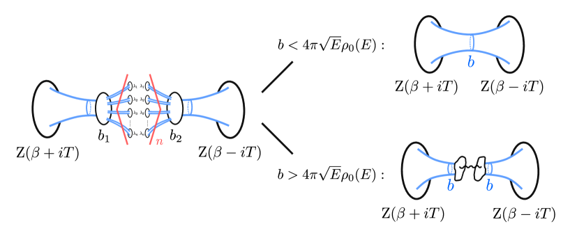
Our last expression for $\langle Z_{B}(b_{1})Z_{B}(b_{2})\rangle_{n}$ results effectively in the following prescription within the gravitational description:

Twist Factor Cutoff.

The twist factor $s$ of a baby universe is bounded by a cutoff of $4\pi\sqrt{E}\rho_{0}(E)$.

• When the size of a baby universes $b$ is smaller than $4\pi\sqrt{E}\rho_{0}(E)$, the baby universe will be traded between the systems and form a wormhole. This results in a connected Riemann surface with a usual twist factor equals to its size $b$.

• When the size of a baby universe is larger than $4\pi\sqrt{E}\rho_{0}(E)$, this baby universes will end on one of the $n$ D-branes in a microcanonical window. The effect of accounting for these non-perturbative D-brane effects is summarized by replacing the twist factor by $4\pi\sqrt{E}\rho_{0}(E)$.

• We draw this cutoff prescription in Fig.8.

Figure 8: Twist factor cutoff.

By construction this cutoff reproduces the ramp-plateau transition of the SFF by allowing the baby universe to end on FZZT branes, as suggested in Saad:2019pqd . Indeed, taking (38) back to (34), we find:

$$\langle|Z(\beta+iT)|^{2}\rangle_{\text{double trumpet}}=\int_{0}^{\infty}db\mathrm{~min}\left\{b,4\pi\sqrt{E}\rho_{0}(E)\right\}\,\psi_{\mathrm{Tr}}(\beta+iT,b)\,\psi_{\mathrm{Tr}}(\beta-iT,b).$$ (41)

Comparing (41) with the genus expansion of JT gravity in (10), we observe that the original twist factor $b$ is replaced by $\mathrm{min}\left\{b,4\pi\sqrt{E}\rho_{0}(E)\right\}$. This implies that when the baby universe is smaller than $4\pi\sqrt{E}\rho_{0}(E)$, we can coarse-graining all D-branes and reproduce the wormhole construction. However, when the size of baby universe exceeds $4\pi\sqrt{E}\rho_{0}(E)$, we can no longer coarse-grain the entire spectrum and need to leave some branes for more precise treatment as D-branes in JT gravity. This results in the twist factor being replaced by $4\pi\sqrt{E}\rho_{0}(E)$, no longer scaling with the size of baby universe.

Figure 9: Emergent ramp-plateau structure when accounting for the $n$ FZZT branes. For $b<4\pi\sqrt{E}\rho_{0}(E)$, the fixed $n$ branes can be coarse-grained together with the $L-n$ branes, and the baby universe form a wormhole, thus reproducing the ramp. For $b>4\pi\sqrt{E}\rho_{0}(E)$, baby universes end on FZZT branes which when integrated over the plateau. This could be visualized as the baby universe ending on effective correlated branes as drawn. Note that this ramp-plateau structure here pertains to the size of baby universes, not time.

We can use the twist factor cutoff prescription to repeat Saad’s wormhole story of the SFF (or correlations functions). At early time, the disk contributions dominate and gives the slope, as no baby universe are exchanged. At later times, the double-trumpet dominates the SFF, allowing the two system to emit or absorb baby universes of any size. The only way to provide a non-decaying return amplitude is by emitting a baby universe of size $T$. For early enough times the baby universes traded are small compared to the twist factor cutoff. Such relatively small baby universes are traded between the two systems and thus include a twist factor is proportional to $T$, giving rise to the ramp. At late enough time, beyond the Heisenberg time, large baby universes take over the job of stopping the decay of the return amplitude. These large baby universe are not able to be traded but rather end on D-branes. Utilizing the resulting twist factor cutoff, they will provide a non-decaying amplitude without extra twist factors to bring in time dependence, recovering the plateau at times beyond the Heisenberg time.

3.5 Effective brane description of the plateau

Regardless of the size of the baby universe, the coarse graining over most of the spectrum leads to non-factorized structure, visible in the delta-function enforcing $b_{1}=b_{2}$. This can be visually represented as in figure 9, where for small $b$ the constraint $b_{1}=b_{2}$ is enforced by having a smooth surface, a wormhole. For large $b$ the non-factorization for is represented by correlated (or entangled) effective branes, similar in spirit to the suggestion in Saad:2019pqd .

In this sense the coarse graining or disorder averaging leads to entanglement, effective branes that are in a Bell pair state. To see this, let us rewrite the SFF in UV picture in (34) by inner products of different states in Hilbert space:

$$|Z(\beta+iT)|_{\text{double trumpet}}^{2} =\Big{(}\langle HH_{\beta+iT}|\otimes\langle HH_{\beta-iT}|\Big{)}\Big{(}|\text{BU}\rangle_{H}\otimes|\text{BU}\rangle_{H}\Big{)},$$ (42)

where $|\text{BU}\rangle_{H}$ represents the baby universe state with inclusion of the FZZT brane contribution:

$$|\text{BU}\rangle_{H}=\int_{0}^{\infty}b~db~Z_{B}(b)~|b\rangle,$$ (43)

and $H$ denotes the dependence of $n\times n$ H matrix in $Z_{B}(b)$. In this UV regime, the two baby universes are not entangled; rather, they contribute as a simple product state, $|\text{BU}\rangle_{H}\otimes|\text{BU}\rangle_{H}$.

At IR, however, disorder averaging brings in delta-function, so that SFF now becomes:

$$\langle|Z(\beta+iT)|^{2}\rangle_{\text{double trumpet}}=\Big{(}\langle HH_{\beta+iT}|\otimes\langle HH_{\beta-iT}|\Big{)}\Big{(}\int_{0}^{\infty}s(b)db~|b\rangle\otimes|b\rangle\Big{)}.$$ (44)

Here, the two baby universes become highly entangled ( large $b$ corresponds to the maximal entanglement and produces plateau). We see that, in the IR, the transition from a factorized geometry to a non-factorized one corresponds to the emergence of entanglement between the two baby universe states. This aligns with the ER=EPR conjecture.

4 Effective time slice and the gray hole conjecture

The modified story of Saad’s wormhole is particularly useful for studying quantities that require non-perturbative completion at all times. It encodes non-perturbative effects coherently while still preserving a clear geometric picture. In this section we calculate the two-point function in the handle-disk geometry, aiming for extracting the probability for the late time Cauchy slice being in a black or white hole state, confirming the ”gray hole conjecture”. We will see how the inclusion of non-perturbative effects through the above twist factor cutoff preserves a clear geometrical picture and ensures that the sum of probabilities is always one at all times. This provides a unified derivation of the gray hole conjecture (for various probes used previously in the literature Stanford:2022fdt ; Blommaert:2024ftn ; Iliesiu:2024cnh ; Miyaji:2024ity ) and extends that to new situations (e.g. with the inclusion matter fields).

4.1 Handle-disk calculation

To this end, let us decompose the two-point function on handle-disk geometry as follows:

$$G_{\Delta}(T) =\sum_{\gamma_{i}=\{\gamma_{1},\gamma_{2},\gamma_{3}\}}\leavevmode\hbox{$\vbox{\hbox{\resizebox{}{}{{\leavevmode\hbox{\set@color{}}}}}}$},$$

$$\approx\int_{\mathcal{F}(b_{1})}db_{1}d\tau_{1}\leavevmode\hbox{$\vbox{\hbox{\resizebox{}{}{{\leavevmode\hbox{\set@color{}}}}}}$}+\int_{\mathcal{F}(b_{2})}db_{2}d\tau_{2}\leavevmode\hbox{$\vbox{\hbox{\resizebox{}{}{{\leavevmode\hbox{\set@color{}}}}}}$},$$

$$=\int_{0}^{\infty}s~db\leavevmode\hbox{$\vbox{\hbox{\resizebox{}{}{{\leavevmode\hbox{\set@color{}}}}}}$}.$$ (45)

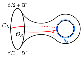
The gravity calculation of the two-point function requires summing over all inequivalent geodesics connecting the boundary operators. Thus in the first line we summed over three classes of geodesics in the bulk geometry. Among these, $\gamma_{3}$ is unaffected by the presence the handle and remains identical to the disk contribution.. Since our interest is late-time behavior of this two-point function while the disk contribution decays, we keep only the $\gamma_{1}$ and $\gamma_{2}$ contributions in the second line. Importantly, to avoid over-counting, the Weil-Petersson measure $b_{i}\wedge\tau_{i}$ for the bulk moduli should be integrated over the fundamental domains of the mapping class group $\mathcal{F}(b_{i})$. However, cutting along $\gamma_{1}$ and $\gamma_{2}$ in each figure yields the same geometry, a two-sided trumpet. Therefore, summing over different geodesics can be achieved instead by integrating over two fundamental domains while fixing the geodesic, as explained in Saad:2019pqd . This simplifies the calculation since $\sum\limits_{i=1}^{2}\int_{\mathcal{F}(b_{i})}db_{i}d\tau_{i}=\int_{0}^{\infty}db\int_{0}^{s}d\tau$, where $s$ is the twist factor. Consequently, in the third line, we can just utilize a single geometry without mapping class group constraints.

Cutting the handle-disk along the geodesic $\gamma_{1}$ results in two-sided trumpet with mixed boundaries:

$$G_{\Delta}(\tau)\supset \frac{e^{-S_{0}}}{Z(\beta)}\int_{-\infty}^{\infty}d\ell\int_{0}^{\infty}s~db\leavevmode\hbox{$\vbox{\hbox{\resizebox{}{}{{\leavevmode\hbox{\set@color{}}}}}}$}e^{-\ell\Delta},$$

$$= \frac{e^{-S_{0}}}{Z(\beta)}\int_{-\infty}^{\infty}d\ell\int_{0}^{\infty}s~db~\psi_{\mathrm{Tr},\beta/2-iT}(\ell,b)~\psi_{\mathrm{Tr},\beta/2+iT}(\ell,b)e^{-\ell\Delta},$$ (46)

$$= \frac{e^{-S_{0}}}{Z(\beta)}\int_{-\infty}^{\infty}d\ell\int_{0}^{\infty}s~db\int_{0}^{\infty}dE_{1}dE_{2}\frac{\mathrm{cos}(b\sqrt{E_{1}})\mathrm{cos}(b\sqrt{E_{2}})}{4\pi^{2}\sqrt{E_{1}E_{2}}}$$

$$\times e^{-(E_{1}+E_{2})\beta/2-i(E_{1}-E_{2})T}\psi_{E_{1}}(\ell)\psi_{E_{2}}(\ell)~e^{-\ell\Delta}.$$ (47)

Under the change of variables $E=\frac{E_{1}+E_{2}}{2}$, $\omega=E_{1}-E_{2}$ and considering a small micro-canonical window with large fixed total energy $E\gg 1$, the two point function simplifies to:

$$G_{\Delta}(T)\supset e^{-S_{0}}\int_{-\infty}^{\infty}d\ell\int_{0}^{\infty}s~db\int_{-\infty}^{\infty}d\omega\frac{\mathrm{cos}(b\sqrt{E+\frac{\omega}{2}})\mathrm{cos}(b\sqrt{E-\frac{\omega}{2}})}{4\pi^{2}E\rho_{0}(E)}$$

$$\times e^{-i\omega T}\psi_{E+\frac{\omega}{2}}(\ell)\psi_{E-\frac{\omega}{2}}(\ell)e^{-\ell\Delta},$$ (48)

$$\approx \int_{-\infty}^{\infty}d\ell\int_{0}^{\infty}s~db\int_{-\infty}^{\infty}d\omega\frac{\mathrm{cos}(b\sqrt{E+\frac{\omega}{2}})\mathrm{cos}(b\sqrt{E-\frac{\omega}{2}})}{4\pi^{2}E\rho_{0}(E)}$$

$$\times e^{-i\omega T}\Theta\left(log(E)+\ell\right)\frac{\mathrm{cos}\left(\frac{\omega}{E^{1/2}}\mathrm{arccossh}(e^{\ell/2}E^{1/2})\right)}{2\pi\rho_{0}(E)(E-e^{-\ell/2})^{1/2}}e^{-\ell\Delta},$$

$$= \int_{-\infty}^{\infty}dT_{\mathrm{eff}}\int_{0}^{\infty}s~db\int_{-\infty}^{\infty}d\omega\frac{\mathrm{cos}(b\sqrt{E+\frac{\omega}{2}})\mathrm{cos}(b\sqrt{E-\frac{\omega}{2}})}{2^{2}\pi^{3}E\rho_{0}^{2}(E)}$$

$$\times e^{-i\omega T}\Theta(T_{\mathrm{eff}})\,\mathrm{cos}(\omega T_{\mathrm{eff}})\,e^{-\ell_{T_{\mathrm{eff}}}\Delta},$$ (49)

where in the second line we used the semiclassical approximation of $\psi_{E+\frac{\omega}{2}}(\ell)\psi_{E-\frac{\omega}{2}}(\ell)$ given in Blommaert:2024ftn , for convenience we include the full derivation in Appendix A. In the last line we define the effective time Blommaert:2024ftn $T_{\mathrm{eff}}=\frac{1}{E^{1/2}}\mathrm{arccosh}(e^{\ell/2}E^{1/2})$. At the large $E$ limit, this transformation matches to Stanford and Yang’s result Yang:2018gdb : $\ell_{T_{\mathrm{eff}}}=2|E^{1/2}T_{\mathrm{eff}}|-\ln 4E$.

An important observation is that both $T_{\mathrm{eff}}$ and $b$ appear inside the cosine function. By expressing the cosine as sum of exponentials, they will both have + branch and - branch. However, $T_{\mathrm{eff}}$ has an additional $\Theta(T_{\mathrm{eff}})$ function, which combines these two branches into a single branch. This ensures that, for a given analytical continuation of T ($>0$), we will not simultaneously obtain a black hole slice ($T_{\mathrm{eff}}>0$) and a white hole slice ($T_{\mathrm{eff}}<0$), unless a baby universe is emitted.

Next we again use the shorthand notation $\mathrm{cos}(x)\mathrm{cos}(y)=\frac{1}{4}e^{(\pm)ix}e^{(\pm)^{\prime}iy}$ where $e^{(\pm)ix}=e^{ix}+e^{-ix}$. Then (49) is cast into the form:

$$G_{\Delta}(T)\supset \int_{-\infty}^{\infty}dT_{\mathrm{eff}}\int_{0}^{\infty}s~db\frac{1}{2^{4}\pi^{2}E\rho_{0}^{2}(E)}\int_{-\infty}^{\infty}\frac{d\omega}{2\pi}e^{i\omega(T_{\mathrm{eff}}-T)}$$

$$\times e^{i\sqrt{E}b\left((\pm)+(\pm)^{\prime}\right)+i\frac{\omega}{4\sqrt{E}}b\left((\pm)-(\pm)^{\prime}\right)}e^{-\ell_{T_{\mathrm{eff}}}\Delta}.$$ (50)

If $(\pm)=(\pm)^{\prime}$, the $e^{\pm i2\sqrt{E}b}$ term won’t survive under the limit $E\gg 1$ and the integration of $b$, thus we are left with $(\pm)=-(\pm)^{\prime}$, giving

$$G_{\Delta}(T)\supset \int_{-\infty}^{\infty}dT_{\mathrm{eff}}~\frac{1}{2^{4}\pi^{2}E\rho_{0}^{2}(E)}\int_{0}^{\infty}s~db\int_{-\infty}^{\infty}\frac{d\omega}{2\pi}e^{i\omega(T_{\mathrm{eff}}-T\pm\frac{1}{2\sqrt{E}}b)}~e^{-\ell_{T_{\mathrm{eff}}}\Delta},$$

$$= \int_{-\infty}^{\infty}dT_{\mathrm{eff}}~\frac{1}{2^{4}\pi^{2}E\rho_{0}^{2}(E)}\int_{0}^{\infty}s~db~\delta(T_{\mathrm{eff}}-T\pm\frac{1}{2\sqrt{E}}b)~e^{-\ell_{T_{\mathrm{eff}}}\Delta},$$

$$= \int_{-\infty}^{\infty}dT_{\mathrm{eff}}~\frac{1}{2\sqrt{E}T_{H}^{2}}~s(b)\Big{|}_{b=\pm 2\sqrt{E}(T_{\mathrm{eff}}-T)}~e^{-\ell_{T_{\mathrm{eff}}}\Delta},$$ (51)

where we identified the Heisenberg time as $T_{H}=2\pi\rho_{0}(E)$. Note that in the third line we replace now $s\rightarrow s(b)$ so that we can now use our twist factor cutoff in Fig.8 to incorporate the late time D-brane effects.

4.2 Incorporating the twist factor cutoff

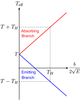
In the final expression (51), the twist factor $s(b)$ plays a role analogous to the conversion factor $\mathcal{F}(T_{\mathrm{eff}}|T)$ defined in Blommaert:2024ftn . For us the conversion factor acquires a very geometric interpretation – the two terms in (51) represent the possibilities of emission or absorption of a baby universe:

• Emitting Branch: $T_{\mathrm{eff}}=T-\frac{1}{2\sqrt{E}}b$.

  The Cauchy slice of two-sided black hole emits a baby universe of size $\frac{1}{2\sqrt{E}}b$, causing the effective time of this slice to be reduced. If $\frac{1}{2\sqrt{E}}b>T$, this emitting process will convert a black hole into a white hole.

• Absorbing Branch: $T_{\mathrm{eff}}=T+\frac{1}{2\sqrt{E}}b$.

  The Cauchy slice of two-sided black hole absorbs a baby universe of size $\frac{1}{2\sqrt{E}}b$, causing the effective time of this slice to increase. This is a time reversed process of emitting a baby universe. This absorbing process will not turn a black hole into a white hole.

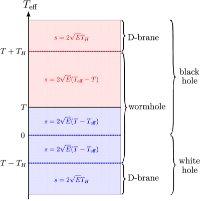
With our prescription the twist factor $s(b)$ is bounded by $2\sqrt{E}T_{H}$ when $b>2\sqrt{E}T_{H}$. The effective time $T_{\mathrm{eff}}$ involves two possible sign choices for $b$, thus the relation between twist factor and $T_{\mathrm{eff}}$ becomes a little involved. We show the relationship between the effective time and the size of the baby universe in fig. 10 and the corresponding twist factor in fig.11. The various possibilities are explained below.

Figure 10: Absorbing Branch (Red) and Emitting Branch (Blue). The black dashed lines represent the twist factor cutoff.

(a) (b)

Figure 11: Twist factor at different effective times with the red region the absorbing branch and the blue region the emitting branch. (a): $T<T_{H}$. (b): $T>T_{H}$.

The probabilities for the late time slice being in a white hole state ($T_{\mathrm{eff}}<0$) or a black holes state ($T_{\mathrm{eff}}>0$) can be extracted from (51) by integrating over the prefactor of the disk two-point function $e^{-\ell_{T_{\mathrm{eff}}}\Delta}$. Below we compute them separately.

White hole probability ($\mathcal{P}_{\mathrm{WH}}$)

The white hole probability arises solely from the emitting branch, with contributions depending on whether the emitted baby universe forms a wormholes or ends on a D-brane.

• For $T<T_{H}$, there are two cases (see Fig.11(a)):

  • $T-T_{H}<T_{\mathrm{eff}}<0$:

    The emitted baby universe forms a wormhole with twist factor $s=2\sqrt{E}(T-T_{\mathrm{eff}})$.

  • $T_{\mathrm{eff}}<T-T_{H}$:

    The emitted baby universe ends on D-brane, with twist factor $s=2\sqrt{E}T_{H}$.

  The probability is then given by:

  $$\mathcal{P}_{\mathrm{WH}}(T) =\frac{1}{T_{H}^{2}}\int_{T-T_{H}}^{0}dT_{\mathrm{eff}}(T-T_{\mathrm{eff}})+\frac{1}{T_{H}^{2}}\int_{-\infty}^{T-T_{H}}dT_{\mathrm{eff}}T_{H},$$

  $$=\frac{T}{T_{H}}-\frac{T^{2}}{2T_{H}^{2}}+\mathrm{const},$$ (52)

  where ”const” is a divergent constant:

  $$\mathrm{const}=-\frac{1}{2}+\frac{1}{T_{H}}\int_{-\infty}^{0}dT_{\mathrm{eff}},$$ (53)

  and needs to be regularized to zero by imposing $\mathcal{P}_{\mathrm{WH}}(T=0)=0$, as in Blommaert:2024ftn .

• For $T>T_{H}$, the only way to tunnel into a white hole is by emitting a large baby universe which then necessarily ends on a D-brane, with twist factor $s=2\sqrt{E}T_{H}$ (see Fig.11(b)). The corresponding probability is:

  $$\mathcal{P}_{\mathrm{WH}}(T) =\frac{1}{T_{H}^{2}}\int_{-\infty}^{0}dT_{\mathrm{eff}}T_{H},$$

  $$=\frac{1}{2}+\mathrm{const}.$$ (54)

Black hole probability ($\mathcal{P}_{\mathrm{BH}}$)

The black hole probability is more complicated. First, we need to include the disk contribution. Using the previous approximations of the wavefunctions, the disk two-point function in a micro-canonical ensemble with $E\gg 1$ is:

$$G_{\Delta}(T)\supset \frac{e^{-S_{0}}}{\rho_{0}(E)}\int_{-\infty}^{\infty}d\ell\int_{0}^{\infty}sdb\int_{-\infty}^{\infty}d\omega\rho_{0}(E+\frac{\omega}{2})\rho_{0}(E-\frac{\omega}{2})e^{-i\omega T}\psi_{E+\frac{\omega}{2}}(\ell)\psi_{E-\frac{\omega}{2}}(\ell)e^{-\ell\Delta},$$

$$\approx \int_{-\infty}^{\infty}dT_{\mathrm{eff}}\delta(T_{\mathrm{eff}}-T)e^{-\ell_{T_{\mathrm{eff}}}\Delta}.$$ (55)

We see that the effective time for the disk is always $T$.

Secondly, the handle-disk geometry now involves both emitting and absorbing branches. Taking these effects into account we can calculate the black hole probability for various times.

• For $T<T_{H}$, there are three cases (see Fig.11(a)):

  • Emitting branch ($0<T_{\mathrm{eff}}<T$):

    The emitted baby universe forms a wormhole, with twist factor $s=2\sqrt{E}(T-T_{\mathrm{eff}})$.

  • Absorbing branch ($T<T_{\mathrm{eff}}<T+T_{H}$):

    The absorbed baby universe comes from a wormhole, with twist factor $s=2\sqrt{E}(T_{\mathrm{eff}}-T)$.

  • Absorbing branch ($T_{\mathrm{eff}}>T+T_{H}$):

    The absorbed baby universe comes from D-brane, with twist factor $s=2\sqrt{E}T_{H}$.

• For $T>T_{H}$, there are four cases (see Fig.11(b)):

  • Emitting branch ($0<T_{\mathrm{eff}}<T-T_{H}$):

    The emitted baby universe ends on D-brane, with twist factor $s=2\sqrt{E}T_{H}$.

  • Emitting branch ($T-T_{H}<T_{\mathrm{eff}}<T$):

    The emitted baby universe comes from a wormhole, with twist factor $s=2\sqrt{E}(T-T_{\mathrm{eff}})$.

  • Absorbing branch ($T<T_{\mathrm{eff}}<T+T_{H}$):

    The absorbed baby universe comes form a wormhole, with twist factor $2\sqrt{E}(T_{\mathrm{eff}}-T)$.

  • Absorbing branch ($T_{\mathrm{eff}}>T+T_{H}$):

    The absorbed baby universe comes form D-brane, with twist factor $s=2\sqrt{E}T_{H}$.

All together , the probability of black hole is:

• $T<T_{H}$:

  $$\mathcal{P}_{\mathrm{BH}}(T)= \int_{0}^{\infty}dT_{\mathrm{eff}}\delta(T_{\mathrm{eff}}-T)+$$

  $$\frac{1}{T_{H}^{2}}\left[\int_{0}^{T}dT_{\mathrm{eff}}(T-T_{\mathrm{eff}})+\int_{T}^{T+T_{H}}dT_{\mathrm{eff}}(T_{\mathrm{eff}}-T)+\int_{T+T_{H}}^{\infty}dT_{\mathrm{eff}}T_{H}\right],$$

  $$=1-\frac{T}{T_{H}}+\frac{T^{2}}{2T_{H}^{2}}+\mathrm{const}.$$ (56)

• $T>T_{H}$:

  $$\mathcal{P}_{\mathrm{BH}}(T)= \int_{0}^{\infty}dT_{\mathrm{eff}}\delta(T_{\mathrm{eff}}-T)+$$

  $$\frac{1}{T_{H}^{2}}\Bigg{[}\int_{0}^{T-T_{H}}dT_{\mathrm{eff}}T_{H}+\int_{T-T_{H}}^{T}dT_{\mathrm{eff}}(T-T_{\mathrm{eff}})+$$

  $$\int_{T}^{T+T_{H}}dT_{\mathrm{eff}}(T_{\mathrm{eff}}-T)+\int_{T+T_{H}}^{\infty}dT_{\mathrm{eff}}T_{H}\Bigg{]}$$

  $$=\frac{1}{2}+\mathrm{const}.$$ (57)

The constant term here is the same as for the white hole case, which is normalized to zero.

Final results

In summary, after regularization, our result for $\mathcal{P}_{\mathrm{WH}}(T)$ and $\mathcal{P}_{\mathrm{BH}}(T)$ is as follows:

$$\textbf{For }\mathbf{T<T_{H}}:\quad\mathcal{P}_{\mathrm{BH}}(T)=1-\frac{T}{T_{H}}+\frac{T^{2}}{2T_{H}^{2}},\quad\mathcal{P}_{\mathrm{WH}}(T)=\frac{T}{T_{H}}-\frac{T^{2}}{2T_{H}^{2}};$$

$$\textbf{For }\mathbf{T\geq T_{H}}:\quad\mathcal{P}_{\mathrm{BH}}(T)=\frac{1}{2},\quad\mathcal{P}_{\mathrm{WH}}(T)=\frac{1}{2};$$ (58)

Our final result matches exactly with Blommaert:2024ftn using the matrix integral. This agreement should not be surprising, since we encode the necessary non-perturbative information into the coarse-graining procedure as we described above.

4.3 Further comments

Below we give several comments on our result:

We see that only the disk and handle-disk geometries with a twist factor cutoff are sufficient to recover the full non-perturbative result. Higher topologies are never important in our treatment, all the non-perturbative effects are encoded in the twist factor cutoff, which in turn is a result of treating the low lying degrees of freedom in gravity as FZZT branes. In Saad:2022kfe the authors used the genus expansion in the $\tau$-scaling limit to recover the plateau. In their treatment higher genus contributions are crucial since they encode the non-perturbative information that leads to the plateau. This does not contradict our treatment which encodes the same non-perturbative effects through FZZT branes.

In our analysis, the Cauchy slice can emit or absorb a baby universe. These two processes comes from the same Euclidean geometry, the handle-disk, which should contribute in a time-symmetric way after analytic continuation to Lorentzian time. As a result, the length of Cauchy slice can also be increased by absorbing a baby universe process. This situation differs somewhat from the analysis in Stanford:2022fdt , where the authors proposed a ”no short-cut” criterion claiming that, in order to correctly identify the interior, distant points along spatial slice should not be close together through the spacetime geometry. Their criterion implies that the correct Cauchy slice should always be the shortest one. However, our result is not in contradiction with theirs – Stanford:2022fdt focuses on the partition function of JT gravity, where careful analysis of the mapping class group is needed to avoid over-counting. The ”no short-cut” criterion is designed to avoid such over-counting. In our case, however, we are calculating two-point function, where all geodesics in the bulk should be summed over. As noted in Saad:2019lba , such summation precisely cancels out the constraints from the mapping class group, leaving the size of baby universe and twist factor unconstrained. Therefore, the ”no short-cut” criterion does not apply to our calculation.

The non-perturbative twist factor cutoff is responsible for normalizing the sum of black hole and white hole probabilities to one at any time, and ensures the saturation to fifty-fifty probability after the Heisenberg time. Geometrically, the saturation comes from the fact that baby universes that lead the Cauchy slice to tunnel into white holes will be large and then necessarily end on D-branes.

In (4.2) we see that the handle-disk topology yields the quadratic term $\frac{T^{2}}{2T_{H}^{2}}$ in the final result in (4.2), while the twist factor cutoff gives the linear term $\frac{T}{T_{H}}$ contribution. This explains why the handle-disk is sufficient to reproduce the $\frac{1}{2}$ probability at the Heisenberg time, as was done by Stanford and Yang Stanford:2022fdt .

It is noteworthy that, in the final expression of black hole probability (4.2), the negative term $-\frac{T}{T_{H}}$ only comes from contributions where the baby universes end on the D-brane in the absorbing branch. However, this does not imply that D-brane somehow decreases the probability for the Cauchy slice to stay in black hole region. Instead, this term appears simply because as $T$ gets larger, the integration region [$T+T_{H}$, $\infty$] narrows. Similarly, the negative term $-\frac{T^{2}}{2T_{H}^{2}}$ in the white hole probability arises also because the integration region $[T-T_{H},0]$ shrinks as $T$ grows (before the Heisenberg time.)

Self-averaging property of the firewall probability.

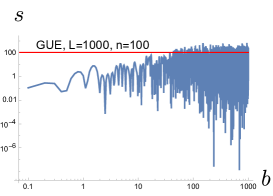
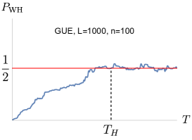
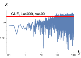
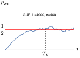
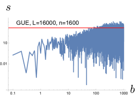
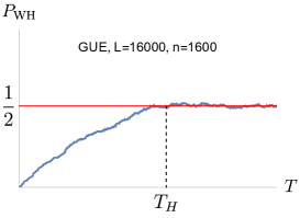
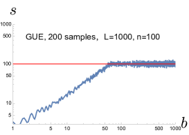
Recall that our effective description involves integrating over configurations of $n$ FZZT branes, after forming an effective theory for these branes by averaging over the fast modes. Suppose we fix a single configuration of these branes, then we may expect the probabilities to be in a black or white hole states to exhibit heavy oscillations, similar to the oscillations of the SFF for a typical draw. This is not the case – this probability involves an integration over the twist factor which acts to smooth the oscillations. As a result we find that the probabilities discussed here are self-averaging in this sense. In the large $n$ limit, the probability approximates the coarse-grained result (4.2). We note that the self-averaging property holds if we fix all eigenvalues and go back to the UV description of a single member of the ensemble. This self-averaging behavior is demonstrated numerically in Fig.12.

Figure 12: Left column: Numerical results for the twist factor s as a function of the baby universe size b. Right column: Numerical results for the white hole probability $\mathcal{P}_{\mathrm{WH}}$ with respect to time $T$. Here, $L$ is the total dimension of GUE matrices, and $n$ denotes the number of fixed (consecutive) eigenvalues drawn from the L$\times$L GUM matrix far from the edge. The first six diagrams display results form single samples, while the last two diagrams showed averaged results over 200 samples. We see that as $L$ and $n$ increase (right column of first six figures), the white hole probability approaches the averaged result, even though the corresponding input — the twist factor – still exhibits significant oscillations (left column of first six figures).

5 Including matter loops

In this section we examine another potential source of firewalls by adding matter loops to our previous discussion, involving the handle-disk geometry with the twist factor cutoff incorporating the effects of FZZT branes. This question was raised in Blommaert:2024ftn – particle-antiparticle pairs created through matter loops on the wormhole geometry may produce dangerous shock waves. Here we will argue that such effects do not alter the firewall probability significantly and should be thought of as renormalizing the vacuum in the presence of wormholes.

We start by discussing the handle-disk without the twist factor cutoff, i.e. when the baby universe exchanged is sufficiently small. The one-loop contribution of a scalar with scaling dimension $\Delta$ is given by Jafferis:2022wez :

$$Z_{\Delta}^{\mathrm{1-loop}}(b) =\prod\limits_{n=0}^{\infty}\frac{1}{1-e^{-b(\Delta+n)}},$$

$$=\sum\limits_{n=0}^{\infty}\frac{e^{-nb\Delta}}{(1-e^{-b})(1-e^{-2b})...(1-e^{-nb})},$$

$$=\mathrm{exp}\left(\sum\limits_{n=1}^{\infty}\frac{e^{-nb\Delta}}{n(1-e^{-nb})}\right),$$ (59)

where $b$ is the size of wormhole throat. The first line is obtained directly from usual CFT quantization on a cylinder, while the second line makes the contributions from primary and descendants states manifest, and the third line shows the divergence at small b.

There are two cycles where one can add a matter loop, corresponding $b_{1}$ and $b_{2}$ depicted in Fig.5. We now discuss them separately.

5.1 Matter loop on $b_{1}$ circle

Adding the matter loop at the cycle $b_{1}$ has no bearing on the firewall probability, since the entire loop remains inside the baby universe and has no contact with the Cauchy slice we denote by $\ell$ and therefore it can not produce shock waves or firewalls. Rather, it simply contributes as a one-loop determinant for the two-point function, which exhibits the well-known divergence at small $b_{1}$, as can be seen from (59). This divergence should be resolved through proper renormalization of fluctuations of the non-trivial topology but this divergence and its renormalization has no effect on the physics governing the emission or absorption of baby universes and the firewall probability (for example it does not depend on the Loretzian time).

We can estimate the finite part of this one-loop determinant by setting $b_{1}$ to its value in the dominant geometry that contributes to the two-point function. Referring to (51), the dominant contribution comes from $\ell_{T_{\mathrm{eff}}}\approx 0$. Combining with $\ell_{T_{\mathrm{eff}}}=2|\sqrt{E}T_{\mathrm{eff}}|-\ln 4E$, the value of $b_{1}$ is:

$$b_{1}=2\sqrt{E}(T-T_{\mathrm{eff}})=2\sqrt{E}T-\ln 4E\approx 2\sqrt{E}T\quad\text{for large T}.$$ (60)

Thus the correction of matter loop at $b_{1}$ at late time can be approximated as:

$$G_{\Delta}^{\mathrm{1-loop}}(T)\approx\mathrm{exp}\left(\sum\limits_{n=1}^{\infty}\frac{e^{-2\sqrt{E}Tn\Delta}}{n(1-e^{-2\sqrt{E}Tn})}\right)\times G_{\Delta}(T),$$ (61)

where $G_{\Delta}(T)$ is the previous two-point function in (51) without the matter loop.

5.2 Matter loop on $b_{2}$ circle

Adding matter loop at the cycle $b_{2}$ is more subtle and relevant, since it intersects with the Cauchy slice $\ell$ and thus can potentially create a dangerous shock wave. Indeed, in the Lorentzian picture depicted in fig.13, where we analytically continue the Euclidean geometry along the time symmetric Cauchy slice $\ell$, a wormhole sends a particle through the matter loop $b_{2}$. If the particle is emitted at early enough time it experiences a large boost and may lead to a dangerous shockwave disrupting the Cauchy slice at late time.

Figure 13: (a) Euclidean picture. (b) Lorentzian picture.

However, we note that the Cauchy slice probed by the late time two-point function, depicted in red in fig.13, always experiences a simultaneous collision with a high energy particle-antiparticle pair, never a collision with a single high energy shock wave. Therefore even though the individual particles are at very high energy, the collision point on the Cauchy slice $\ell$ will remain in a vacuum state rather than a firewall state.

We elaborate on this conclusion by arguing for the non-existence of a firewall in two ways: first, by calculating the soft modes of the two-point function in the handle-disk geometry, as in Stanford:2021bhl , and second, by comparing the situation to the two-sided eternal AdS black hole, where it clearly leads to vacuum renormalization rather than a firewall.

5.2.1 Soft modes in the two-point function

A straightforward way to determine whether a dangerous shockwave exists is to check if the Dray- ’t Hooft shockwave action can be extracted at late time. To do this, we start by expressing two-point function (48) using the angular variables in Appendix A as:

$$G_{\Delta}(T)\supset~ e^{-S_{0}}\int_{-\infty}^{\infty}d\ell\int_{0}^{\infty}db\int_{-\infty}^{\infty}d\omega\int_{-\infty}^{\infty}d\alpha_{1}d\alpha_{2}~s~\frac{\mathrm{cos}(b\sqrt{E+\frac{\omega}{2}})\mathrm{cos}(b\sqrt{E-\frac{\omega}{2}})}{4\pi^{2}E\rho_{0}(E)}$$

$$\times e^{-2e^{-\frac{\ell}{2}}\left(\mathrm{cosh}(\alpha_{1})+\mathrm{cosh}(\alpha_{2})\right)}e^{-2iE^{1/2}(\alpha_{1}+\alpha_{2})}e^{-2i\frac{\omega}{4E^{1/2}}(\alpha_{2}-\alpha_{1})}e^{-i\omega T-\ell\Delta},$$

$$=~ \frac{e^{S_{0}}}{4\pi^{2}E\rho_{0}(E)}\int_{-\infty}^{\infty}d\ell\int_{0}^{\infty}db\int_{-\infty}^{\infty}d\omega\int_{-\infty}^{\infty}d\alpha_{1}d\alpha_{2}~s$$

$$\times\mathrm{exp}\Bigg{[}i\omega\bigg{(}(\pm)\frac{b}{4E^{1/2}}-(\pm)^{\prime}\frac{b}{4E^{1/2}}-T-\frac{1}{2E^{1/2}}(\alpha_{1}-\alpha_{2})\bigg{)}+$$

$$ib\bigg{(}(\pm)E^{1/2}+(\pm)^{\prime}E^{1/2}\bigg{)}+2iE^{1/2}(\alpha_{1}+\alpha_{2})-2e^{-\frac{\ell}{2}}\left(\mathrm{cosh}(\alpha_{1})+\mathrm{cosh}(\alpha_{2})\right)\Bigg{]}.$$ (62)

There are five integration variables and the corresponding saddle point equations are:

$$\ell:\quad e^{-\frac{\ell}{2}}\left(\mathrm{cosh}(\alpha_{1})+\mathrm{cosh}(\alpha_{2})\right)=0.$$

$$b:\quad(\pm)\frac{\omega}{4E^{1/2}}-(\pm)^{\prime}\frac{\omega}{4E^{1/2}}+(\pm)E^{1/2}+(\pm)^{\prime}E^{1/2}=0.$$

$$\omega:\quad(\pm)\frac{b}{4E^{1/2}}-(\pm)^{\prime}\frac{b}{4E^{1/2}}-T-\frac{1}{2E^{1/2}}(\alpha_{1}-\alpha_{2})=0.$$

$$\alpha_{1}:\quad-\frac{i\omega}{2E^{1/2}}+2iE^{1/2}-2e^{-\frac{\ell}{2}}\sinh(\alpha_{1})=0.$$

$$\alpha_{2}:\quad\frac{i\omega}{2E^{1/2}}+2iE^{1/2}-2e^{-\frac{\ell}{2}}\sinh(\alpha_{2})=0.$$ (63)

The solutions of the above set of equations only exist when $(\pm)=-(\pm)^{\prime}$. In that case, the solutions are:

$$\omega=0;\quad\alpha_{1}=i\frac{\pi}{2}-\left(E^{1/2}T\pm\frac{b}{2}\right);\quad\alpha_{2}=i\frac{\pi}{2}+\left(E^{1/2}T\pm\frac{b}{2}\right);$$

$$e^{-\frac{\ell}{2}}\cosh(E^{1/2}T\pm\frac{b}{2})=E^{1/2};\quad b:\text{unfixed}.$$ (64)

Note that the value of $b$ remains unfixed, i.e. we obtain a family of solutions parametrized by $b$. This represents a soft mode, corresponding to the size of the baby universe (the circle $b_{1}$). This soft mode exists for any time $T$.

In order to obtain shockwave modes at late times, new soft modes should emerge as $T\gg 1$. For example, in Stanford:2021bhl , the radial coordinates of the OTOC contour on the hyperbolic disk are no longer constrained by the saddle point equations at late times. These new soft modes recover the Dray-’t Hooft shockwave action and thus represent high-energy shockwave collisions at late times.

In our case, however, since $b$ is always a soft mode, we must sum over contributions from all sizes of b. As a result, the late time limit can always be effectively reduced by $\frac{b}{2}$ so that $E^{1/2}T-\frac{b}{2}\sim 0$. Consequently, the saddle point equations are not sensitive to the large $T$ limit, and no new soft modes can emerge in that limit.

For consistency, we can check that the large $T$ limit of (64) recovers the previous result of the effective time slice: $\ell=|2E^{1/2}T\pm b|-\ln 4E$. The effective action at the saddle point is then simply:

$$\mathrm{exp}\left[-2\pi E^{1/2}\right]$$ (65)

which matches the result in Appendix A without the one-loop determinant. Therefore, no Dray-’ t Hooft type action arises at late times and thus there are no possible sources for a dangerous firewall.

5.2.2 Analogy with the eternal black hole

We can also see the non-existence of a firewall directly from the Penrose diagram of the Loretzian process. We start by discussing an analogous and familiar situation for the eternal black hole, depicted in fig.14. We then argue that our situation is identical.

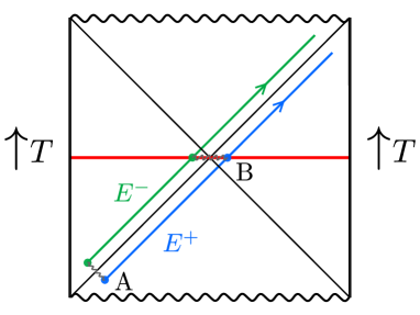
Consider the two-sided eternal AdS black hole, we define the bulk Hamiltonian to be $H=H_{L}+H_{R}$ so that both sides evolve upwards , as drawn in Fig.14. In that Penrose diagram, the early vacuum fluctuation at region $A$ produce an entangled Hawking pair: one particle with positive energy $E^{+}$ inside the white hole and another with negative energy $E^{-}$ outside the white hole horizon. Under Lorentzian evolution, both particles are blue shifted along the horizon before $T=0$ and then red shifted after that time. As a result, on the $T=0$ time slice (region $B$ in the figure), both Hawking particles appear to be highly energetic. However, this does not indicate the presence of a firewall. The entangled pair represents a vacuum state along the horizon, which is Lorentz invariant. Despite $E^{+}$ and $E^{-}$ being separately blue shifted, their combined energy always cancels out. Therefore, regions $A$ and $B$ are in the same vacuum state with equal net vacuum energy. There is no firewall.

Figure 14:

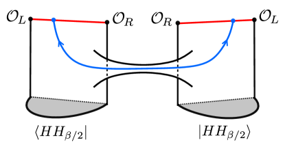
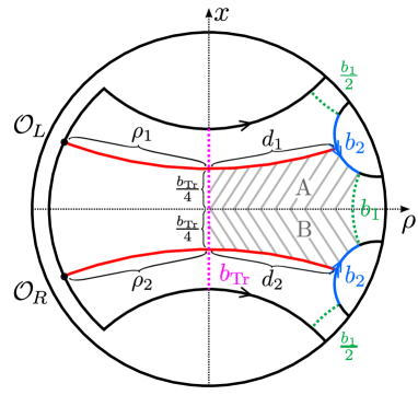
The above argument applies directly to our matter loop case, as we will now argue. Consider Fig.13(a), the time directions of the left and right systems (both in the thermofield double state) are chosen opposite, which is natural in the presence of the bra and ket Hartle-Hawking states in the two-point function. In other words with this choice we are calculating an in-in correlator using a Schwinger-Keldyish contour. This is similar to the left and right boundaries in the analogous situation for two-side AdS black hole discussed above. Meanwhile, the moduli space of handle-disk geometry has SL(2,R) gauge redundancy and we choose the gauge so that the handle is $\mathbb{Z}_{2}$ symmetric with respect to the geodesic $\ell$ (or more precisely, twisting over $b_{\mathrm{Tr}}$ in Fig.17), see Appendix B.

For the bulk viewpoint, in order to ensure that the Cauchy slice $\ell$ properly describes the black hole or white hole interior (depending on the size of the baby universe) in both systems, we need to flip the sign of the Hamiltonian in one of the systems. The upshot of both arguments is that for the calculation of the two-point function the time direction should be drawn as in Fig. 15(a).

Figure 15: Energy fluxes on the matter loop.(a) two systems with opposite time direction. (b) two systems with same time direction.

Thus, in Fig.15(a), the time directions of the two systems are opposite. Also note that, due to the $\mathbb{Z}_{2}$ symmetry in handle-disk geometry, the wormhole in the Lorentzian picture is parallel to the Cauchy slice. The entangled particle pair is created at region A, with one particle being radiated to left system with positive energy $E^{+}$. Under Lorentzian time evolution, this particle crosses the Cauchy slice and is finally annihilated by its entangled partner at region B. This may lead us to suspect that the emitted particle in the left system collides with the Cauchy slice at high energy and therefore resembles a firewall.

However, this interpretation is incomplete. We need to also analyze this process from the perspective of the right system. In the right system, the Cauchy slice is not hit by any particle. Instead, since the wormhole is parallel to the Cauchy slice, it radiates a particle with the same high energy as the particle that collides with the Cauchy slice in the left system, which is later absorbed by the wormhole at region B with energy $E^{+}$. Combining the perspectives from both side, the Cauchy slice is actually ”transparent” to this excited particle. There is no momentum transfer in this ”collision”.

An alternative bulk picture is presented in Fig.15(b) by choosing the time evolution in both systems to align. In this case, an entangled particle pair with positive and negative energies as drawn, is created at region A. This pair may experience large blue shift but it is ultimately annihilated on the Cauchy slice at region B. This is the same as our analogous situation in Fig.14, where the vacuum state at region A evolves into the vacuum at region B. In that analogous case, Lorentz invariance ensures that region B on the Cauchy slice remains a vacuum state, instead of a firewall. Similarly, on the bulk Cauchy slice relevant for the two-point function we encounter short distance divergences which should be interpreted as part of the definition of the vacuum in the presence of a wormhole.

For completeness, we can also approximate the one-loop determinant on the $b_{2}$ circle using the same method as in the $b_{1}$ case. The location of $b_{2}$ makes the calculation more complicated and we show the detailed derivation in Appendix.B. It turns out, the dominant geometry corresponds to $b_{2}\rightarrow\infty$, meaning that the one-loop determinant here is just unity. Therefore, the two-point function approximately equals to the one without the matter loop:

$$G_{\Delta}^{\mathrm{1-loop}}(T)\approx G_{\Delta}(T).$$ (66)

This supports the idea that the matter loop does not cause large changes in the probe two-point function, and should be thought of merely as renormalization effects.

5.3 Large baby universes

The discussion thus far is relevant for matter loops in the presence of sufficiently small baby universes, such that the effective gravitational description is a wormhole. For completeness we can discuss the matter loop for large baby universes which end on one of our FZZT branes.

We argue that aside for the treatment of the twist factor the conclusions are identical. To this end we use the picture of correlated effective branes, resulting from the integration over the FZZT branes, which are found to be maximally entangled (see (44)). We can therefore define the matter loop as the probe matter field operator acting on these maximally entangled states,

$$|\delta\Delta\rangle\equiv\int_{0}^{\infty}s(b)~db~\delta\mathcal{O}_{\Delta}\cdot\Big{(}|b\rangle\otimes|b\rangle\Big{)}.$$ (67)

The maximal entanglement in the large $b$ basis ensures that the matter loop carries through smoothly, resulting effectively in a matter loop, whether we are in the smooth wormhole regime or the correlated branes, both contain a delta function ( see (44)) restricting to $b_{1}=b_{2}$. The only difference is the treatment of the twist factor $s(b)$. This we conclude that our previous statement applies, the effect of matter loops represent vacuum fluctuations rather than a firewall.

6 Summary and future directions

We use the framework of JT gravity together with FZZT branes as as an effective Wilsonian description of the matrix integral, as described in in Sec.3. This provides a natural framework of encoding non-perturbative effects long time effects into the genus expansion. This approach allows us to complete the wormhole shortening picture with the full non-perturbative corrections summarized by an effective twist factor with a cutoff. The effective twist factor separates the D-brane and wormhole contributions at any time and preserves a clear geometric picture.

By applying this twist factor cutoff prescription to the two-point function on the handle-disk geometry, we find that the white hole probability increases at late time and eventually saturates to $1/2$ after the Heisenberg time. This validates the gray hole conjecture and indicates a 1/2 possibility for an in-falling observer to encounter a firewall behind horizon at late time. This result remains valid even for a single quantum system without ensemble averaging. Meanwhile, through soft mode analysis and analogy with the eternal black hole, we find that the matter loops in the handle-disk geometry do not produce any further firewall. Instead, they correspond to a vacuum renormalization effect in topologically non-trivial spacetimes.

There are several interesting future directions. The notion of firewall should be quantified more precisely bu constructing a precise model for an infalling observer, perhaps along the lines of Jafferis:2022wez ; Gao:2021tzr ; deBoer:2022zps . The twist factor cutoff can be also used for other dilaton gravity model that do not have a clear matrix dual. In particular it would be interesting to examine the finite $\sigma$ setup discussed in Blommaert:2021gha . This corresponds to the situation where only a few FZZT branes are inserted into the micro-canonical windows. In this case, we might expect that the double trumpet and two-point functions to undergo a ”tearing phase” transitions with extra macroscopic holes Kazakov:1989cq . In such case, the two-point function lacks a clear genus expansion, making it difficult to maintain a clear geometric picture. However, it may still be possible to encode the dual deformed matrix integral results into the effective twist factor. On the gravity side, we can still use the handle-disk geometry with this effective twist factor to calculate the firewall probability. It would be interesting to check if how the firewall probability might be modified during this tearing phase transition.

Appendix A Semiclassical approximation of $\psi_{E+\frac{\omega}{2}}(\ell)\,\psi_{E-\frac{\omega}{2}}(\ell)$

In this appendix we derive the approximation of the expression $\psi_{E+\frac{\omega}{2}}(\ell)\psi_{E-\frac{\omega}{2}}(\ell)$ in micro-canonical ensemble with large $E$, following Blommaert:2024ftn . First we express the wavefunction in terms of the modified Bessel functions and use the integral representation:

$$K_{i\alpha}(x)=\frac{1}{2}\int_{-\infty}^{\infty}dbe^{-x\mathrm{cosh}b}e^{-i\alpha b}.$$ (68)

Giving,

$$\psi_{E+\frac{\omega}{2}}(\ell)\psi_{E-\frac{\omega}{2}}(\ell) =2K_{2i\sqrt{E-\frac{\omega}{2}}}\left(2e^{-\ell/2}\right)2K_{2i\sqrt{E+\frac{\omega}{2}}}\left(2e^{-\ell/2}\right),$$

$$=\int_{-\infty}^{\infty}db_{1}db_{2}e^{-2e^{-\frac{l\ell}{2}}\mathrm{cosh}(b_{1})}e^{-2e^{-\frac{\ell}{2}}\mathrm{cosh}(b_{2})}e^{-2i(E-\frac{\omega}{2})^{\frac{1}{2}}b_{1}}e^{-2i(E+\frac{\omega}{2})^{\frac{1}{2}}b_{2}},$$

$$\approx\int_{-\infty}^{\infty}db_{1}db_{2}e^{-2\left(e^{-\frac{\ell}{2}}\mathrm{cosh}(b_{1})+e^{-\frac{\ell}{2}}\mathrm{cosh}(b_{2})\right)}e^{-2iE^{1/2}(b_{1}+b_{2})}e^{-2i\frac{\omega}{4E^{1/2}}(b_{2}-b_{1})}.$$ (69)

Relabeling the variables,

$$\pi-2ib_{1}=2iE^{1/2}(G+g),\quad\pi-2ib_{2}=2iE^{1/2}(-G+g).$$ (70)

the integral (69) becomes:

$$2E\int_{-\infty}^{\infty}dGdg\exp{\bigg{\{}-2\pi E^{1/2}+4iEg-i\omega G-i2\left[e^{-\frac{\ell}{2}}\mathrm{sinh}\left(E^{\frac{1}{2}}(G+g)\right)+e^{-\frac{\ell}{2}}\mathrm{sinh}\left(E^{\frac{1}{2}}(-G+g)\right)\right]\bigg{\}}}.$$ (71)

The saddle point equations of $G$ and $g$ for this integral are:

$$\frac{\partial S}{\partial g}\Bigg{|}_{g=g_{\star}}=0,\quad\frac{\partial S}{\partial G}\Bigg{|}_{G=G_{\star}}=0\quad\Rightarrow$$

$$(4E-\omega)=4E^{1/2}e^{-\frac{\ell}{2}}\mathrm{cosh}(E^{1/2}(G_{\star}+g_{\star})),\quad(4E+\omega)=4E^{1/2}e^{-\frac{\ell}{2}}\mathrm{cosh}(E^{1/2}(-G_{\star}+g_{\star})),$$ (72)

with two solutions ($\omega\rightarrow 0$):

$$G_{\star} =\frac{\mathrm{arccosh}(E^{1/2}e^{\frac{\ell}{2}})}{E^{1/2}},\quad g_{\star}=0;$$

$$\quad\mathrm{or}:G_{\star}\rightarrow-G_{\star},\quad g_{\star}\rightarrow-g_{\star}.$$ (73)

Note that the above solution is only valid when $E^{1/2}e^{\frac{\ell}{2}}\geq 1$. So we need to add Heaviside function $\Theta\left(\log(E)+\ell\right)$ to the result.

The on-shell action is obtained as:

$$S_{\star}= -2\pi E^{1/2}\pm\frac{i\omega}{E^{1/2}}\mathrm{arccosh}(E^{1/2}e^{\frac{\ell}{2}}).$$ (74)

One-loop determinant for this saddle point is given as:

$$\mathrm{det}\left(\begin{array}[]{cc}\frac{\partial^{2}S}{\partial G\partial G}&\frac{\partial^{2}S}{\partial G\partial g}\\ \frac{\partial^{2}S}{\partial g\partial G}&\frac{\partial^{2}S}{\partial g\partial g}\end{array}\right)\Bigg{|}_{G=G_{\star},g=g_{\star}}=16E^{2}(E-e^{-\ell}).$$ (77)

All in all, including two sets of saddle points and one-loop determinant contributions, the wavefunction product can be approximated as:

$$\psi_{E+\frac{\omega}{2}}(\ell)\psi_{E-\frac{\omega}{2}}(\ell)\approx \frac{2\pi}{\sqrt{E-e^{-\ell}}}\exp{(-2\pi E^{1/2})}\mathrm{cos}\left(\frac{\omega}{E^{1/2}}\mathrm{arccosh}(e^{\frac{\ell}{2}}E^{1/2})\right)\Theta\left(\log(E)+\ell\right),$$

$$\approx \frac{e^{S_{0}}}{2\pi\sqrt{E-e^{-\ell}}\rho_{0}(E)}\mathrm{cos}\left(\frac{k}{E^{1/2}}\mathrm{arccosh}(e^{\frac{\ell}{2}}E^{1/2})\right)\Theta\left(\log(E)+\ell\right),$$ (78)

where in the second approximation we used the fact that $E\gg 1$ so $\mathrm{exp}(-2\pi E^{\frac{1}{2}})\approx\frac{e^{S_{0}}}{4\pi^{2}\rho_{0}(E)}$.

Appendix B One-loop determinant of the $b_{2}$ circle

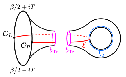
To calculate the one-loop determinant of $b_{2}$, it is more convenient to decompose the handle-disk geometry as shown in Fig.16, into a trumpet with one asymptotic boundary and one geodesic boundary of size $b_{\mathrm{Tr}}$ and a pair of pants with three geodesic boundaries: $b_{\mathrm{Tr}}$, $b_{2}$, $b_{2}$, where we sum over all the values of $b_{2}$.

Figure 16:

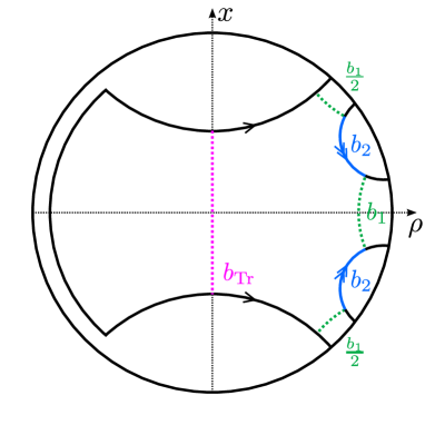
To perform the calculation, we present the handle-disk geometry as a quotient of the hyperbolic disk in Fig.17. We work with the Fermi coordinates:

$$ds^{2}=d\rho^{2}+\mathrm{cosh}^{2}\rho dx^{2},$$ (79)

where the trumpet region has $\rho<0$ (left hand side of $b_{\mathrm{Tr}}$) and the pair of pants region has $\rho>0$ (right hand side of $b_{\mathrm{Tr}}$) with two boundaries $b_{1}$ being glued together.

Figure 17:

To find the value of $b_{2}$ after analytically continuing the two-point function to Lorentztian time $T$, we use the same method as in the $b_{1}$ case by matching Euclidean data to the dominant contribution at late times. The case of $b_{2}$ is more complicated since it depends on both $b_{1}$ and $b_{\mathrm{Tr}}$. Let us now calculate the circle $b_{2}$ and the length of Cauchy slice $\ell$ in terms $b_{1}$ and $b_{\mathrm{Tr}}$ on this hyperbolic disk.

B.1 Length of $\ell$

The two boundary operators $\mathcal{O}_{L}$ and $\mathcal{O}_{R}$ are inserted at asymptotic boundary symmetrically with respect to the center of the coordinate system. Semi-classically, we can parametrize the coordinates of the boundary operators as:

$$\mathcal{O}_{L}:(-\rho_{1},b_{Tr}/4),\quad\mathcal{O}_{R}:(-\rho_{2},-b_{Tr}/4).$$ (80)

The length of $\ell$ can be decomposed as follows:

$$\ell=\rho_{1}+\rho_{2}+d_{1}+d_{2}.$$ (81)

Figure 18:

We can calculate $d_{1}$ and $d_{2}$ using trigonometry of the pentagons A and B in Fig.18 10.1007/978-0-8176-4992-0 :

$$\cosh\frac{b_{1}}{2}=\sinh\frac{b_{\mathrm{Tr}}}{4}\sinh d_{1}=\sinh\frac{b_{\mathrm{Tr}}}{4}\sinh d_{2}.$$ (82)

This gives the length of $d_{1}$ and $d_{2}$:

$$e^{d_{1}}=e^{d_{2}}=\frac{\cosh\frac{b_{1}}{2}}{\sinh\frac{b_{\mathrm{Tr}}}{4}}+\sqrt{\frac{\cosh^{2}\frac{b_{1}}{2}}{\sinh^{2}\frac{b_{\mathrm{Tr}}}{4}}+1}$$ (83)

Thus, the total length of $\ell$ is:

$$e^{\ell}=\left(\frac{\cosh\frac{b_{1}}{2}}{\sinh\frac{b_{\mathrm{Tr}}}{4}}+\sqrt{\frac{\cosh^{2}\frac{b_{1}}{2}}{\sinh^{2}\frac{b_{\mathrm{Tr}}}{4}}+1}\right)^{2}e^{\rho_{1}+\rho_{2}}$$ (84)

Note that $\rho_{1}$ and $\rho_{2}$ simply shift the value of $\ell$. Since in the two-point function $\ell$ in integrated over, we can absorb the dependence of $\rho_{1}+\rho_{2}$ by a redefinition: $\ell\rightarrow\ell-\rho_{1}-\rho_{2}$.

B.2 Length of $b_{2}$

We can calculate $b_{2}$ via the following Hexagon on the hyperbolic disk:

Figure 19:

The sides satisfy:

$$\cosh\frac{b_{\mathrm{Tr}}}{2}=\sinh^{2}\frac{b_{1}}{2}\cosh b_{2}-\cosh^{2}\frac{b_{1}}{2}.$$ (85)

So length of $b_{2}$ is obtained as:

$$\mathrm{cosh}b_{2}=\frac{\mathrm{cosh}\frac{b_{\mathrm{Tr}}}{2}+1}{\mathrm{sinh}^{2}\frac{b_{1}}{2}}+1.$$ (86)

B.3 One-loop determinant

In sum, we have three related formulas:

$$e^{\ell}=\left(\frac{\mathrm{cosh}\frac{b_{1}}{2}}{\mathrm{sinh}\frac{b_{Tr}}{4}}+\sqrt{\frac{\mathrm{cosh}^{2}\frac{b_{1}}{2}}{\mathrm{sinh}^{2}\frac{b_{\mathrm{Tr}}}{4}}+1}\right)^{2},\quad(\text{hyperbolic data})$$ (87)

$$\mathrm{cosh}b_{2}=\frac{\mathrm{cosh}\frac{b_{\mathrm{Tr}}}{2}+1}{\mathrm{sinh}^{2}\frac{b_{1}}{2}}+1,\quad(\text{hyperbolic data})$$ (88)

$$\ell_{T_{\mathrm{eff}}}=|2T\sqrt{E}\pm b_{1}|-\mathrm{ln}4E=0,\quad(\text{Lorentzian saddle})$$ (89)

Solving the above equations we find:

$$b_{1}=2T\sqrt{E}-\ln 4E,\quad b_{\mathrm{Tr}}\rightarrow\infty,\quad b_{2}\rightarrow\infty.$$ (90)

Thus, it turns out that the one-loop determinant on the circle $b_{2}$ is simply unity on the saddle geometry:

$$Z_{\Delta}^{\text{1-loop}}(b_{2}\rightarrow\infty)=1.$$ (91)

References

- (1) S.W. Hawking, Particle Creation by Black Holes, Commun. Math. Phys. 43 (1975) 199.
- (2) S.W. Hawking, Breakdown of Predictability in Gravitational Collapse, Phys. Rev. D 14 (1976) 2460.
- (3) T. Banks, W. Fischler, S.H. Shenker and L. Susskind, M theory as a matrix model: A conjecture, Phys. Rev. D 55 (1997) 5112 [hep-th/9610043].
- (4) J.M. Maldacena, The Large N limit of superconformal field theories and supergravity, Adv. Theor. Math. Phys. 2 (1998) 231 [hep-th/9711200].
- (5) S.S. Gubser, I.R. Klebanov and A.M. Polyakov, Gauge theory correlators from noncritical string theory, Phys. Lett. B 428 (1998) 105 [hep-th/9802109].
- (6) E. Witten, Anti-de Sitter space and holography, Adv. Theor. Math. Phys. 2 (1998) 253 [hep-th/9802150].
- (7) A. Almheiri, D. Marolf, J. Polchinski and J. Sully, Black Holes: Complementarity or Firewalls?, JHEP 02 (2013) 062 [1207.3123].
- (8) A. Almheiri, D. Marolf, J. Polchinski, D. Stanford and J. Sully, An Apologia for Firewalls, JHEP 09 (2013) 018 [1304.6483].
- (9) R. Bousso, Complementarity Is Not Enough, Phys. Rev. D 87 (2013) 124023 [1207.5192].
- (10) Y. Nomura, J. Varela and S.J. Weinberg, Complementarity Endures: No Firewall for an Infalling Observer, JHEP 03 (2013) 059 [1207.6626].
- (11) J. Maldacena and L. Susskind, Cool horizons for entangled black holes, Fortsch. Phys. 61 (2013) 781 [1306.0533].
- (12) M. Van Raamsdonk, Evaporating Firewalls, JHEP 11 (2014) 038 [1307.1796].
- (13) A. Almheiri, X. Dong and D. Harlow, Bulk Locality and Quantum Error Correction in AdS/CFT, JHEP 04 (2015) 163 [1411.7041].
- (14) X. Dong, D. Harlow and A.C. Wall, Reconstruction of Bulk Operators within the Entanglement Wedge in Gauge-Gravity Duality, Phys. Rev. Lett. 117 (2016) 021601 [1601.05416].
- (15) A. Almheiri, R. Mahajan, J. Maldacena and Y. Zhao, The Page curve of Hawking radiation from semiclassical geometry, JHEP 03 (2020) 149 [1908.10996].
- (16) G. Penington, S.H. Shenker, D. Stanford and Z. Yang, Replica wormholes and the black hole interior, JHEP 03 (2022) 205 [1911.11977].
- (17) A. Almheiri, T. Hartman, J. Maldacena, E. Shaghoulian and A. Tajdini, Replica Wormholes and the Entropy of Hawking Radiation, JHEP 05 (2020) 013 [1911.12333].
- (18) A. Almheiri, N. Engelhardt, D. Marolf and H. Maxfield, The entropy of bulk quantum fields and the entanglement wedge of an evaporating black hole, JHEP 12 (2019) 063 [1905.08762].
- (19) G. Penington, Entanglement Wedge Reconstruction and the Information Paradox, JHEP 09 (2020) 002 [1905.08255].
- (20) L. Susskind, ER=EPR, GHZ, and the consistency of quantum measurements, Fortsch. Phys. 64 (2016) 72 [1412.8483].
- (21) J.M. Maldacena, Eternal black holes in anti-de Sitter, JHEP 04 (2003) 021 [hep-th/0106112].
- (22) S.H. Shenker and D. Stanford, Black holes and the butterfly effect, JHEP 03 (2014) 067 [1306.0622].
- (23) J.S. Cotler, G. Gur-Ari, M. Hanada, J. Polchinski, P. Saad, S.H. Shenker et al., Black Holes and Random Matrices, JHEP 05 (2017) 118 [1611.04650].
- (24) P. Saad, S.H. Shenker and D. Stanford, JT gravity as a matrix integral, 1903.11115.
- (25) P. Saad, S.H. Shenker and D. Stanford, A semiclassical ramp in SYK and in gravity, 1806.06840.
- (26) P. Saad, Late Time Correlation Functions, Baby Universes, and ETH in JT Gravity, 1910.10311.
- (27) A. Blommaert, T.G. Mertens and H. Verschelde, Clocks and Rods in Jackiw-Teitelboim Quantum Gravity, JHEP 09 (2019) 060 [1902.11194].
- (28) C. Yan, Crosscap contribution to late-time two-point correlators, JHEP 12 (2023) 051 [2203.14436].
- (29) D. Stanford and Z. Yang, Firewalls from wormholes, 2208.01625.
- (30) L. Susskind, The Typical-State Paradox: Diagnosing Horizons with Complexity, Fortsch. Phys. 64 (2016) 84 [1507.02287].
- (31) A. Blommaert, C.-H. Chen and Y. Nomura, Firewalls at exponentially late times, 2403.07049.
- (32) L.V. Iliesiu, A. Levine, H.W. Lin, H. Maxfield and M. Mezei, On the non-perturbative bulk Hilbert space of JT gravity, JHEP 10 (2024) 220 [2403.08696].
- (33) M. Miyaji, Discrete Spectrum of Interior Length and Timeshift in Two-sided Black Hole, 2410.20662.
- (34) G. Sárosi, AdS2 holography and the SYK model, PoS Modave2017 (2018) 001 [1711.08482].
- (35) D.A. Trunin, Pedagogical introduction to the Sachdev–Ye–Kitaev model and two-dimensional dilaton gravity, Usp. Fiz. Nauk 191 (2021) 225 [2002.12187].
- (36) T.G. Mertens and G.J. Turiaci, Solvable models of quantum black holes: a review on Jackiw–Teitelboim gravity, Living Rev. Rel. 26 (2023) 4 [2210.10846].
- (37) D.L. Jafferis, D.K. Kolchmeyer, B. Mukhametzhanov and J. Sonner, Jackiw-Teitelboim gravity with matter, generalized eigenstate thermalization hypothesis, and random matrices, Phys. Rev. D 108 (2023) 066015 [2209.02131].
- (38) A. Goel, L.V. Iliesiu, J. Kruthoff and Z. Yang, Classifying boundary conditions in JT gravity: from energy-branes to -branes, JHEP 04 (2021) 069 [2010.12592].
- (39) D. Stanford and E. Witten, Fermionic Localization of the Schwarzian Theory, JHEP 10 (2017) 008 [1703.04612].
- (40) Z. Yang, The Quantum Gravity Dynamics of Near Extremal Black Holes, JHEP 05 (2019) 205 [1809.08647].
- (41) D. Harlow and D. Jafferis, The Factorization Problem in Jackiw-Teitelboim Gravity, JHEP 02 (2020) 177 [1804.01081].
- (42) A. Blommaert, T.G. Mertens and H. Verschelde, Eigenbranes in Jackiw-Teitelboim gravity, JHEP 02 (2021) 168 [1911.11603].
- (43) B. Post, J. van der Heijden and E. Verlinde, A universe field theory for JT gravity, JHEP 05 (2022) 118 [2201.08859].
- (44) A. Altland, B. Post, J. Sonner, J. van der Heijden and E.P. Verlinde, Quantum chaos in 2D gravity, SciPost Phys. 15 (2023) 064 [2204.07583].
- (45) R. Dijkgraaf and C. Vafa, Matrix models, topological strings, and supersymmetric gauge theories, Nucl. Phys. B 644 (2002) 3 [hep-th/0206255].
- (46) R. Dijkgraaf and C. Vafa, On geometry and matrix models, Nucl. Phys. B 644 (2002) 21 [hep-th/0207106].
- (47) A. Blommaert, L.V. Iliesiu and J. Kruthoff, Gravity factorized, JHEP 09 (2022) 080 [2111.07863].
- (48) A. Blommaert, Dissecting the ensemble in JT gravity, JHEP 09 (2022) 075 [2006.13971].
- (49) P. Saad, S.H. Shenker, D. Stanford and S. Yao, Wormholes without averaging, JHEP 09 (2024) 133 [2103.16754].
- (50) P. Saad, S.H. Shenker and S. Yao, Comments on wormholes and factorization, JHEP 10 (2024) 076 [2107.13130].
- (51) F. Haake, Quantum Signatures of Chaos, Springer Series in Synergetics, Springer, Berlin (2010), 10.1007/978-3-642-05428-0.
- (52) M.L. Mehta, Random Matrices, 3rd ed. (2004).
- (53) P. Saad, D. Stanford, Z. Yang and S. Yao, A convergent genus expansion for the plateau, JHEP 09 (2024) 033 [2210.11565].
- (54) D. Stanford, Z. Yang and S. Yao, Subleading Weingartens, JHEP 02 (2022) 200 [2107.10252].
- (55) W. Fischler and L. Susskind, Dilaton Tadpoles, String Condensates and Scale Invariance, Phys. Lett. B 171 (1986) 383.
- (56) P. Gao and L. Lamprou, Seeing behind black hole horizons in SYK, JHEP 06 (2022) 143 [2111.14010].
- (57) J. de Boer, D.L. Jafferis and L. Lamprou, On black hole interior reconstruction, singularities and the emergence of time, 2211.16512.
- (58) A. Blommaert and J. Kruthoff, Gravity without averaging, SciPost Phys. 12 (2022) 073 [2107.02178].
- (59) V.A. Kazakov, A Simple Solvable Model of Quantum Field Theory of Open Strings, Phys. Lett. B 237 (1990) 212.
- (60) P. Buser, Geometry and spectra of compact riemann surfaces, .