MorphiNet: A Graph Subdivision Network for Adaptive Bi-ventricle Surface Reconstruction

Abstract

Cardiac Magnetic Resonance (CMR) imaging is widely used for heart modelling and digital twin computational analysis due to its ability to visualize soft tissues and capture dynamic functions. However, the anisotropic nature of CMR images, characterized by large inter-slice distances and misalignments from cardiac motion, poses significant challenges to accurate model reconstruction. These limitations result in data loss and measurement inaccuracies, hindering the capture of detailed anatomical structures. This study introduces MorphiNet, a novel network that enhances heart model reconstruction by leveraging high-resolution Computer Tomography (CT) images, unpaired with CMR images, to learn heart anatomy. MorphiNet encodes anatomical structures as gradient fields, transforming template meshes into patient-specific geometries. A multi-layer graph subdivision network refines these geometries while maintaining dense point correspondence. The proposed method achieves high anatomy fidelity, demonstrating approximately 40% higher Dice scores, half the Hausdorff distance, and around 3 mm average surface error compared to state-of-the-art methods. MorphiNet delivers superior results with greater inference efficiency. This approach represents a significant advancement in addressing the challenges of CMR-based heart model reconstruction, potentially improving digital twin computational analyses of cardiac structure and functions.

Cardiac magnetic resonance, Digital twin, Mesh reconstruction, Gradient field, Graph neural network.

1 Introduction

Digital heart models, represented as 3D meshes reconstructed from medical imaging, are valuable for investigating cardiac physiology and evaluating treatments through simulations that replicate the heart’s characteristics [1, 2]. Cardiovascular Magnetic Resonance (CMR) imaging is commonly used for digital heart reconstruction because it can visualize soft tissues, provide detailed anatomical structural information, and capture dynamic cardiac functions with high temporal resolution and signal-to-noise ratio without ionizing radiation. However, accurate model reconstruction from CMR data is challenging due to its anisotropic nature, resulting from the balance between relatively slow data acquisition and scanning time constraints. This anisotropy presents as large inter-slice distances. Additionally, differences in breath-hold positioning between slices (i.e., motion artefacts) can further misalign the data, ultimately producing incomplete and imprecisely registered information [3]. Although fully volumetric (3D) CMR acquisitions can mitigate slice misalignment issues, that challenge persists in the imaging formats routinely used in clinical practice. Precise anatomical structures and dimensions are critical for clinical assessments. For instance, inaccuracies in the cavity or myocardial wall dimensions can result in misdiagnoses of conditions such as heart failure or hypertrophy. Although super-resolution and advanced interpolation techniques offer improvements, [4, 5], current methods often struggle to restore true geometries of the cardiac structure lost or distorted between slices. Besides, their over-reliance on limited training datasets fails to capture the full variability of heart anatomy and motion, ultimately affecting the accuracy of functional analyses [6].

Explicit reconstruction methods, which define surfaces using vertices, edges, and faces to form a mesh, are generally preferred for 3D heart modelling due to their ability to create structured meshes with dense point correspondence, providing an efficient representation of the heart’s physiological characteristics [7]. These methods offer advantages over computationally intensive implicit techniques [8], which require long inference times. Explicit reconstruction methods define surfaces using vertices, edges, and faces to form a coherent mesh. They’re generally preferred for 3D heart modelling, as they produce structured meshes with dense point correspondence. This structure supports an efficient representation of the heart’s physiological characteristics [7]. In contrast, implicit techniques [8] tend to be more computationally intensive and often require much longer inference times. Chen et al. developed a deep-learning model for real-time 3D mesh reconstruction with improved accuracy and robustness but relied on high-quality training data to address reconstruction challenges from CMR images [9]. Voxel2Mesh [10] employed graph convolutional networks (GCN) to convert volumetric data into 3D meshes, demonstrating improved anatomical accuracy but facing variability across patient datasets. Similarly, Kong et al. [11] used GCNs for whole-heart mesh reconstruction by warping a template across cases. Recently, the ModusGraph framework [12] was introduced to automate 3D and 4D mesh model reconstruction from cine CMR, using multi-modal learning and signed distance sampling. However, the issue of performance degradation on unseen data persists, particularly when precise anatomical structures and dimensions are not rigorously modelled.

In this paper, we address the challenges posed by the anisotropic nature of CMR images by proposing an efficient method to restore missing structural information about the heart, as shown in Fig 1. The critical step is to learn the true underlying anatomy as prior knowledge and use this knowledge to infer the specific patient’s heart shape. We found that Computed Tomography (CT) imaging naturally conveys prior knowledge due to its higher spatial resolution despite its lower temporal resolution. We introduce MorphiNet, which learns the true anatomy from unpaired CMR and CT image data and automatically performs patient-specific tuning to generate accurate heart models.

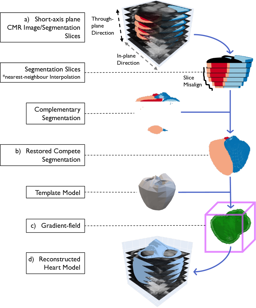
Figure 1: Overview of the proposed MorphiNet framework. From top to down: a) Start with the anisotropic nature of cardiac magnetic resonance images with large inter-slice distances and misalignments. b) Restoration of true cardiac anatomy. c) Find a gradient field from the segmentation to adjust the template mesh. d) End with a reconstructed heart model preserving underlying cardiac anatomy while conforming to patient-specific data.

We argue that previous explicit reconstruction methods are inadequate because their deformation processes fail to guarantee accurate anatomical structures. These methods optimise deformation by minimising the Chamfer distance [13] between a deformed mesh and the ground truth segmentation or point cloud. While this reduces the average distance from each vertex to its nearest ground truth point, it doesn’t establish one-to-one correspondences or ensure accurate curvature or surface continuity. As a result, these reconstructions may look close on average but fail to capture the true anatomical geometry precisely. Instead, MorphiNet decodes the true anatomy as a gradient field, guiding the deformation of a template mesh to match specific heart geometries. Additionally, we apply adaptive subdivision and deformation with a Graph Subdivision Network (GSN) to refine geometries in complex surface areas while maintaining a dense point correspondence. Our proposed method offers an explainable and efficient solution to incorporate accurate anatomical structures into heart model reconstructions. Our main contributions are,

• To our knowledge, we are the first to provide a 3D mesh reconstruction method from anisotropic CMR images with a learned, controllable and traceable surface subdivision and deformation procedure.

• We ensure accurate anatomical structures by a gradient-field mesh adjustment process with a learned true underlying cardiac anatomy.

• Our method, MorphiNet, performs better than state-of-the-art baselines in four different whole-heart medical image datasets regarding anatomy fidelity.

• We demonstrate its potential in modelling the heart function in a motion-tracking task and scrutinize its performance with extensive ablation studies.

This paper extends our previous work [14] in the following ways: it introduces updates to the methodology by incorporating dynUNet for segmentation and ResNet for anatomical restoration, providing a detailed and transparent pipeline description. It elaborates on adaptive mesh refinement using a Graph Subdivision Network (GSN). It describes its multi-layer perceptron-based vertex adjustment and presents new mathematical formulations for template deformation and subdivision. The experimental section is expanded with an additional dataset, the Automatic Cardiac Diagnosis Challenge (ACDC), and it updates experiment results and evaluation scores to assess mesh quality comprehensively. Detailed visualizations, including surface error maps and cross-sectional overlays, enhance the presentation of results. At the same time, extensive ablation studies and a more granular comparative analysis against state-of-the-art methods highlight MorphiNet’s performance and contributions.

2 Related Work

2.1 Statistical Shape Model

Statistical shape modelling (SSM) in cardiology is a computational technique used to analyze and represent the variability in the shape of cardiac structures across populations. Young et al. [15] used interactive finite element 3D shape models to streamline the calculation of left ventricular mass and volume. More automated approaches extended to multiple chambers and the development of 3D statistical shape models [16]. The introduction of 4D atlases by Perperidis et al. [17] captured dynamic cardiac changes and distinguished between inter- and intra-subject variability. SSMs are essential for computational cardiac atlases [18], enhancing personalized medicine and epidemiological studies of biophysical properties. Large-scale studies by Medrano-Gracia et al. [19] and Bai et al. [20] demonstrated the value of extensive datasets, constructing detailed atlases that enable analysis of population shape variations. The integration of multiple imaging modalities, as shown by Puyol-Antón et al. [21], and the application of SSM to myocardial infarction classification by Suinesiaputra et al. [22], enhanced the clinical applicability. Gilbert et al. [23] reviewed machine learning in cardiac atlasing to improve automation and precision. Recent advancements include applications to pediatric cardiology, with Marciniak et al. [24] identifying morphological changes linked to childhood obesity and Govil et al. [25] achieving fully automated modelling for congenital heart disease using deep learning.

2.2 Learning-based Approaches

Deep learning-based methods for mesh reconstruction in cardiology are unified by their data-driven learning approaches, which excel at feature extraction and representation from complex cardiac imaging data, and their robustness and adaptability to varying patient-specific and modality-specific inputs. Xu et al. [26] reformulated the problem through volumetric mapping, enabling flexible handling of multi-orientation contours without mesh constraints. Kong et al. [11] addressed topology preservation challenges in cardiac reconstruction, targeting issues of disconnected regions and anatomical inconsistencies. Chen et al. [9] focused on handling sparse point clouds using learned deformation registration. Beetz et al. [27] introduced point cloud completion networks, achieving significant error reduction and cross-domain adaptability on public datasets. Taking a different approach, Meng et al. [28] developed region-specific mesh tracking for cardiac dynamics, while Yuan et al. [29] separated shape and motion modelling using implicit representations. Deng et al. [12] combined voxel processing with graph convolution networks to enhance motion capture for biomechanical studies. Neural implicit methods have emerged as another direction: Verhülsdonk et al. [30] enabled continuous shape generation across imaging modalities, Stolt-Ansó et al. [31] proposed continuous space segmentation for sparse data, and Muffoletto et al. [32] demonstrated robust reconstruction from limited standard CMR views. Addressing specific clinical needs, Kong et al. [33] developed shape-disentangled modelling for congenital heart defects with virtual cohort generation capabilities. While explicit methods directly represent cardiac surfaces through mesh parameterization, enabling efficient point correspondence and real-time reconstruction crucial for clinical applications, implicit methods offer flexibility in handling topological variations but face challenges in computational efficiency and surface extraction, particularly when dense point correspondence is required for motion tracking and biomechanical analysis.

3 Method

MorphiNet is a fully automatic, end-to-end pipeline to generate a 3D mesh model, shown as the flow in blue in Fig 2. Taking a stack of short-axis (SAX) CMR images as input, a dynUNet segmentation network [34] (a MONAI [35] implementation of nnU-Net [36]) infers three specific heart regions – left ventricle (LV), right ventricle (RV), and myocardium (Myo) – from the image. A ResNet decoder [37] predicts a complementary segmentation, which restores segmentations near the basal and apex plane that are missing from the CMR stack. The complete segmentation is transformed into a distance map. A gradient field is derived from the distance map and is used to deform a template mesh, adjusting the mesh to conform with the actual anatomical structure in the input patient data. Following this, an Adaptive Subdivision Process with GSN layers refines the adjusted template mesh by increasing the number of surface points and encouraging finer surface adjustments. The result is a 3D mesh model with a smooth surface and dense points.

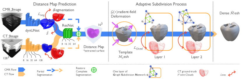
Figure 2: Diagram of forward propagation in MorphiNet for heart reconstruction from CMR images. From left to right: 1) A dynUNet generates segmentation from the stack of SAX CMR images. The segmentation is downsampled, and a complementary segmentation from the ResNet restores the underlying cardiac anatomy. 2) This complete segmentation is then converted to a distance map with Euclidian distance transformation, derived from which a gradient field is imposed on a template mesh to perform patient-specific adjustment; an Adaptive Subdivision Process with GSN layers deforms and refines the adjusted template mesh into a dense 3D mesh model.

3.1 Distance Map Prediction

We denote the cardiac images as a signal intensity function $\mathcal{I}:\mathbf{\Omega}\mapsto\mathbb{R}$ of voxels in the domain $\mathbf{\Omega}\subseteq\mathbb{R}^{3}$, and the ground truth segmentation of heart structures as a mapping $f:\mathcal{I}\subseteq\mathbb{R}\mapsto\mathcal{S}\in\{1,2,3\}$ from the intensity to one of the three heart regions (LV, RV & Myo). Two dynUNets with the same structure are individually employed for CMR and CT segmentation. The dynUNets are structured with five down-size convolution layers, four up-size isotropic convolution layers, a bottleneck of 128 channels and a size of $4\times 4\times 4$. Both take uncropped image volumes and infer segmentation in a sliding window manner, implemented using sliding_window_inference from MONAI [38]. The segmentation is downsampled to equalise the in-plane and through-plane resolutions. This approach mitigates the anisotropic nature of CMR data and minimises resolution differences between CMR and CT data. The segmentation from each dynUNet is denoted as $\hat{\mathcal{S}}=f(\mathcal{I};\theta_{\text{u}})$, where dynUNet’s parameters $\theta_{\text{u}}$ are optimised by reducing the Dice loss [39] with the ground truth segmentation.

We assume cardiac anatomy is consistent across imaging modalities but is observed differently in CMR and CT images. Unlike the CT image, the ventricular cardiac anatomy in the CMR image (in Fig 1) is incomplete due to the absence of critical slices near the apex and basal plane. Moreover, aliasing appears due to the large slice-to-slice distance, and slice misalignments caused by cardiac motion are evident. The previous segmentation and downsampling approach mitigates the aliasing and misalignments, but critical slices must be restored. Therefore, we used a ResNet to predict a complementary segmentation from dynUNet’s output to restore those critical slices. This ResNet was trained solely on CT segmentation from CT dynUNet’s output, where slices near the apex and basal plane are masked. It is optimised by minimising the Dice loss between the restored and the ground truth segmentations. Eventually, the dynUNet’s segmentation and the ResNet restoration are complementary and convey the underlying cardiac anatomy. The distance map results from a Euclidian distance transform applied to the complete segmentation, implemented using distance_transform_edt from MONAI.

3.2 Adaptive Subdivision Process

Based on a subdivision shape modelling process elaborated in [40], we adapted a biventricular template mesh $\mathcal{M_{\text{c}}}=\left(\mathcal{V},\mathcal{F}\right)$ for left and right ventricular myocardium muscle, with 388 vertices ($\mathcal{V}=388$) and 780 faces ($\mathcal{F}=780$). Each vertex is assigned an anatomical label as one of LV endocardium, RV endocardium, LV epicardium, RV epicardium, or valve. This mesh was defined in the Normalised Device Coordinates (NDC), where the mesh’s size is bounded in the $\left[-1,1\right]$ range and centred at the space origin.

Algorithm 1 Graph Subdivision Network (GSN)

Input: Meshes $\mathcal{M}$

Output: Updated Meshes

for $l=1$ to 2 do

     $\text{edge\_verts}\leftarrow\text{ComputeEdgeMidpoints}(\mathcal{M})$

     $\text{new\_verts}\leftarrow\text{Concatenate}(\mathcal{M}.\text{verts},\text{edge\_verts})$

     $\mathcal{M}\leftarrow\text{CreateMeshes}(\text{new\_verts},\text{new\_faces})$

     $\text{deg}\leftarrow\text{ComputeDegree}(\mathcal{M}.\text{edges})$

     for edge $(i,j)$ in $\mathcal{M}.\text{edges}$ do

         $\text{norm}\leftarrow 1/\sqrt{\text{deg}[i]\cdot\text{deg}[j]}$

         $\text{diff}\leftarrow\mathcal{M}.\text{verts}[j]-\mathcal{M}.\text{verts}[i]$

         $\text{message}\leftarrow h_{\theta_{\text{m}}}(\text{diff})$

         $\text{update}[i]\leftarrow\text{update}[i]+\text{norm}\cdot\text{message}$

     end for

     $\mathcal{M}\leftarrow\text{OffsetVertices}(\mathcal{M},\text{update})$

     Add $\mathcal{M}$ to output list

end for

return output

Adjusting $\mathcal{M_{\text{c}}}$ in the gradient field follows a two-step procedure visualised in Fig 3. The first step is aligning $\mathcal{M_{\text{c}}}$ with the myocardium segmentation by the RV centroid. This is fulfilled by applying a rigid, “swing” rotation to the $\mathcal{M_{\text{c}}}$. The RV centroid is the key point for the registration, which is found from the RV epicardial surface of $\mathcal{M_{\text{c}}}$. The myocardium segmentation is translated and scaled to NDC, where the corresponding RV centroid coordinate is found. Because the long axis (from the tricuspid valve to the LV apex) of $\mathcal{M_{\text{c}}}$ must be parallel with that of the myocardium segmentation and Z-axis, we can rotate $\mathcal{M_{\text{c}}}$ along the Z-axis by an angle of $\phi$ to complete the alignment. The angle between the RV centroids’ projection on XY-plane determines $\phi$. Through experiments, we find this rigid, “swing” rotation by RV centroid registration results in the best preliminary shape alignment. The second step is a gradient-field mesh deformation. In the distance map, we find the gradient field by calculating the first- or second-order estimates of partial derivatives at every coordinate $\bm{p}\in\mathbb{R}^{3}\times\left[-1,1\right]$, implemented using torch.gradient from PyTorch [41]. Three partial derivatives $\left(\partial\bm{p}/\partial x,\partial\bm{p}/\partial y,\partial\bm{p}/\partial z\right)$ determine the gradient vector $\mathcal{G}\left(\bm{p}\right)$. Adjusting the $\mathcal{M_{\text{c}}}$ is performed by moving its vertices in the gradient field by iterations. This results in a smooth trajectory that leads each vertex to the zero gradient position to match the underlying surface. This adjustment process is performed on vertices with the same anatomical label and individually for each anatomical label group. For most cases, after 10 iterations, the shape of the $\mathcal{M_{\text{c}}}$ is stabilised. This adjustment process is implemented in algorithm 2.

Algorithm 2 Adjust Template Mesh $\mathcal{M_{\text{c}}}$

Input: Gradient Field Predictions $\mathcal{G}$, Template Mesh $\mathcal{M_{\text{c}}}$

Output: Adjusted Template Mesh $\mathcal{M_{\text{c}}}$

Step 1: Rigid “Swing” Rotation Alignment

$\text{RV\_c}\leftarrow\text{ComputeRVCentroid}(\mathcal{M_{\text{c}}})$

$\text{RV\_c\_seg}\leftarrow\text{GetSegmentationRVCentroid}(\mathcal{G})$

$R\leftarrow\text{ComputeRotationMatrix(RV\_c, RV\_c\_seg)}$

$\mathcal{M_{\text{c}}}.\text{verts}\leftarrow\text{ApplyRotation}(\mathcal{M_{\text{c}}}.\text{verts},R)$

Step 2: Gradient-Field Mesh Deformation

for each label in [LV-epi, LV, RV, RV-epi] do

     $\text{verts\_idx}\leftarrow\text{GetVerticesWithLabel}(\mathcal{M_{\text{c}}},\text{label})$

     $\mathcal{G}_{\text{label}}\leftarrow\mathcal{G}[\text{label}]$

     for iteration = 1 to 10 do

         $\text{offset}\leftarrow\text{SampleGradient}(\mathcal{G}_{\text{label}},\mathcal{M_{\text{c}}}.\text{verts}[\text{verts\_idx}])$

         $\mathcal{M_{\text{c}}}.\text{verts}[\text{verts\_idx}]\leftarrow\mathcal{M_{\text{c}}}.\text{verts}[\text{verts\_idx}]+\text{offset}$

     end for

end for

return $\mathcal{M_{\text{c}}}$

Our GSN structure, inspired by the Loop subdivision [42], refines the mesh by splitting edges to form new triangles and updating vertices to approximate intricate heart geometries. In the Loop subdivision, the updated vertex $\bm{v}^{\prime}$ relative to the original vertex $\bm{v}_{i}$ comes from a calculation considering its neighbours $\mathcal{N}(\bm{v}_{i})$ as

$$\bm{v}^{\prime}_{i} =(1-\alpha\cdot\text{deg}(i))\bm{v}_{i}+\alpha\sum_{\bm{v}_{j}\in\mathcal{N}(\bm{v}_{i})}\bm{v}_{j}$$

$$=\bm{v}_{i}+\sum_{\bm{v}_{j}\in\mathcal{N}(\bm{v}_{i})}\alpha(\bm{v}_{j}-\bm{v}_{i})$$ (1)

where $\text{deg}(i)$ is the vertex’s degree, and $\alpha$ is a weight defined by Warren’s formula [43]. Splitting edges end up with new vertices – the mid-points of those edges.

In this study, we avoid mesh shrinkage and provide more deformation freedom in our GSN structure. GSN updates both original and new vertices following equations in Loop subdivision but substituting $\alpha$ with a three-layer, 16 hidden-feature optimisable multi-layer perceptron $h_{\theta_{\text{m}}}$ and normalising the weighted sum by vertex’s degree. This update to all vertices is formalised as,

$$\mathrm{\Delta}\bm{v}_{i}=\sum_{\bm{v}_{j}\in\mathcal{N}(\bm{v}_{i})}\frac{1}{\sqrt{\text{deg}(i)}\cdot\sqrt{\text{deg}(j)}}\cdot h_{\theta_{\text{m}}}\left(\bm{v}_{j}-\bm{v}_{i}\right)$$ (2)

and a multi-layer GSN implemented in algorithm 1.

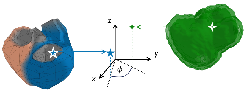
(a) Step 1: Rigid “swing” rotation

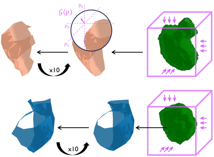
(b) Step 2: Gradient field deformation

Figure 3: The patient-specific adjustment applied to the template model. (a) A rigid “swing” rotation is determined to register the RV centroid of the template mesh with that of the myocardium segmentation. (b) The gradient field is transformed from the distance map and is used to deform the template mesh iteratively along the gradient vectors. The gradient field deformation is applied individually to groups of the template mesh’s vertices categorized by their anatomical label. Only LV and RV epicardium are shown in the figures for ease of demonstration.

In practice, the new vertices are appended to the original ones at each subdivision level, and their anatomical label is determined jointly by neighbouring vertices. This subdivision ensures a fixed mesh topology. It also ensures a simple scheme to link new vertices with the original vertices at each subdivision level and keep track of the anatomical label whilst adding new vertices.

We optimised the GSN by minimising a Chamfer distance [13] between the generated dense 3D mesh model $\hat{\mathcal{M}}=\left(\hat{\mathcal{V}},\hat{\mathcal{F}}\right)$ and the ground truth point clouds. These point clouds $\mathcal{P}^{\prime}$ are extracted from the ground truth segmentation. The Chamfer distance $\mathcal{L}_{\text{Chmf}}(\hat{\mathcal{M}},\mathcal{P}^{\prime})$ is minimized along with Laplacian smoothing [44] $\mathcal{L}_{\text{Lap}}(\hat{\mathcal{M}})$,

$$\mathcal{L}_{\text{Chmf}}(\hat{\mathcal{M}},\mathcal{P}^{\prime}) =\sum_{i=0}^{N}{\frac{1}{\left|\hat{\mathcal{V}_{i}}\right|}\sum_{v\in\hat{\mathcal{V}}_{i}}{\min_{p\in\mathcal{P}^{\prime}_{i}}{\left|v-p\right|}_{2}^{2}}}$$

$$+\sum_{i=0}^{N}{\frac{1}{\left|\mathcal{P}^{\prime}_{i}\right|}\sum_{p\in\mathcal{P}^{\prime}_{i}}{\min_{v\in\hat{\mathcal{V}}_{i}}{\left|p-v\right|}_{2}^{2}}}$$ (3)

$$\mathcal{L}_{\text{Lap}}(\hat{\mathcal{M}}) =\sum_{v_{i}\in\hat{\mathcal{V}}}\frac{\left(\cot{a}_{ij}+\cot{b}_{ij}\right)}{4A_{i}}\left(v_{i}-v_{j}\right)$$ (4)

where $v$ is vertices with the i-th anatomical label in $\hat{\mathcal{M}}$ and $p$ is the points’ position in $\mathcal{P}^{\prime}$ extracted from the ground truth segmentation corresponding to that anatomical label; ${a}_{ij}$ and ${b}_{ij}$ are the “outside” angles in the two triangles connecting vertex $v_{i}$ and its neighbouring vertex $v_{j}$, and $A_{i}$ is the sum of the areas of all triangles containing vertex $v_{i}$, implemented using chamfer_distance and mesh_laplacian_smoothing from PyTorch3D [45].

3.3 Optimisation

We empirically apply weight coefficients $\mathrm{\lambda}_{0}=0.56$ and $\mathrm{\lambda}_{0}=0.12$ to balance the loss components in the total loss for training, given by

$$\mathcal{L}=\mathcal{L}_{\text{seg}}+\mathrm{\lambda}_{0}\cdot\mathcal{L}_{\text{Chmf}}+\mathrm{\lambda}_{1}\cdot\mathcal{L}_{\text{Lap}}$$ (5)

We implemented a training scheme for heart reconstruction from either CT or CMR image data. The two dynUNets were trained for CMR and CT image segmentation with minimised Dice loss. With the downsampled CT segmentation, the ResNet is trained to restore and complete CT segmentation from masked input segmentation. A distance map is derived by applying Euclidian distance transformation to that complete segmentation. Following the adjustment process described in section 3.2, a template mesh is adjusted to a patient-specific shape. The GSN is optimised with minimised Chamfer distance and Laplacian smooth regularisation (3) and (4). Except for training a dynUNet for CMR segmentation, no other part of MorphiNet requires a single CMR case for training.

4 Experiment

4.1 Experimental Setup

We evaluated MorphiNet on four datasets: a subset with 232 CT scans randomly chosen from the Scottish Computed Tomography of the Heart (SCOT-HEART) dataset [46], a subset with 222 CMR scans randomly chosen from the Cardiac Atlas Project (CAP) dataset [25], and two external validation sets – the Multi-Modality Whole Heart Segmentation (MMWHS) with 20 CT scans [47] and a subset with 20 CMR scans randomly chosen from the Automatic Cardiac Diagnosis Challenge (ACDC) [48]. After random scattering, an 80-20 training/testing split is applied to the CAP and SCOT-HEART datasets, respectively. All images were interpolated through bilinear interpolation, and all manual segmentations were interpolated through the nearest-neighbour interpolation. Both result in a $2\ \text{mm}\times 2\ \text{mm}\times 2\ \text{mm}$ resolution. The data augmentation included Gaussian noise with a standard deviation of 0.01, Gaussian smoothing with an isotropic kernel of 0.25 mean and 1.5 standard deviations, and intensity scaling with a factor of 1.3 – all operations were applied with 0.15 possibility to individual data.

MorphiNet was trained using the AdamW optimizer [49] with an initial learning rate of 0.001 for 300 epochs: 100 for dynUNets, 80 for ResNet, and 120 for GSN. The training and testing were conducted on an NVIDIA RTX 3090 GPU, the same as all baseline methods. For comparison, we implemented four baseline methods: Voxel2Mesh [10], ModusGraph [12], CorticalFlow++ [50], and Neural Deformation Field (NDF) [51]. All methods used identical training/testing datasets and preprocessing and post-processing steps for fair comparison. A Laplacian smoothing filter $(\lambda=0.13)$ is applied to all methods’ results to the generated models for preferable surface smoothness. Methods except MorphiNet require a region of interest cropping, resizing and zeros padding to $128^{3}$ pixel-size volumes. Methods except NDF use the identical template mesh described in section 3.1. NDF’s generated models were obtained by extracting the zero-level set and applying the marching cubes algorithm, followed by a surface decimation to control the number of vertex and faces. Although marching cubes result in high accuracy measured by the performance metrics in Table 1, the resulting meshes cannot be used for digital heart modelling due to a lack of correspondence between cases. Therefore, NDF is a “target benchmark” in performance metric comparisons.

4.2 Surface Reconstruction Performance

We first evaluated MorphiNet’s reconstruction capability on both CT and CMR datasets. Dice score (Dice) and Hausdorff distance (Hd) [52] measured errors between voxelized, generated models from all methods and ground truth segmentations, implemented from https://github.com/cvlab-epfl/voxel2mesh. All voxelized, generated models and ground truth segmentations are $128^{3}$ pixel-size volume. Average Surface Distance (AVD) [53] measured the minimum Euclidean distances between the generated models’ surface and 5,000 points uniformly sampled from the ground truth segmentation, where 5,000 is the average number of vertices on the generated models. Aspect Ratio (AspR), scaled Jacobian Ratio (JacR) – both were checked using compute_cell_quality in pyvista, Mean Normal Consistency (MnC) and Non-manifold Faces Ratio (NmF) [51] were chosen for mesh quality evaluation. GPU Inference Time (InFt) is the average time to generate a mesh model from CT/CMR images.

Fig. 4 demonstrates the surface reconstruction results on SCOT-HEART and MMWHS datasets, showing the generated models with surface error visualizations. Table 1 presents the quantitative comparison with baseline methods, where we assessed geometric accuracy and mesh quality metrics. For CMR reconstruction from CAP and ACDC datasets, we evaluated short-axis (SAX) and long-axis (LAX) views where ground truth segmentations are available. Fig. 5 illustrates the reconstruction results across different cardiac views, with model cross-sections overlaid on the ground truth segmentations. The performance metrics are summarized in Table 2.

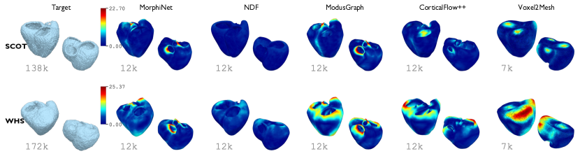
Figure 4: Surface reconstruction results on SCOT-HEART and MMWHS datasets, with the highest face count per method displayed in the bottom left and coloured with surface errors (mm). The RV myocardium segmentation in the MMWHS dataset grows from RV epicardium, resulting in a 3 mm-thick myocardium free-wall segmentation.

Table 1: Evaluation results on SCOT-HEART and MMWHS datasets.

Dataset	Method	Dice$\uparrow$	Hd$\downarrow$	ASD$\downarrow$	AspR$\downarrow$	JacR$\uparrow$	MnC$\uparrow$	NmF$\downarrow$	InFt$\downarrow$
	$\diamond$Voxel2Mesh	$0.38\left(0.04\right)$	$5.25\left(0.99\right)$	$4.61\left(0.62\right)$	$\textbf{1.36}\left(0.01\right)$	$0.72\left(0.01\right)$	$0.73\left(0.02\right)$	$1.02\left(0.01\right)$	$0.33$
	$\diamond$CortFlow++	$0.28\left(0.06\right)$	$8.08\left(1.15\right)$	$3.24\left(0.57\right)$	$1.43\left(0.01\right)$	$0.69\left(0.00\right)$	$0.76\left(0.01\right)$	$\textbf{0.04}\left(0.00\right)$	$1.18$
SCOT	$\diamond$ModusGraph	$0.47\left(0.06\right)$	$5.82\left(1.12\right)$	$3.87\left(0.61\right)$	$1.39\left(0.00\right)$	$\textbf{0.75}\left(0.00\right)$	$0.76\left(0.01\right)$	$\textbf{0.04}\left(0.00\right)$	0.08
	$\diamond$MorphiNet	$\textbf{0.73}\left(0.02\right)$	$\textbf{2.55}\left(0.31\right)$	$\textbf{2.84}\left(0.49\right)$	$1.49\left(0.02\right)$	$0.66\left(0.01\right)$	$\textbf{0.77}\left(0.01\right)$	$\textbf{0.04}\left(0.00\right)$	$1.34$
	$\dagger$NDF	$0.79\left(0.06\right)$	$1.99\left(0.75\right)$	$0.89\left(0.13\right)$	$1.40\left(0.02\right)$	$0.70\left(0.01\right)$	$0.81\left(0.01\right)$	$0.00\left(0.00\right)$	$122.64$
	$\diamond$Voxel2Mesh	$0.42\left(0.08\right)$	$6.84\left(0.89\right)$	$5.84\left(0.90\right)$	$1.39\left(0.02\right)$	$0.71\left(0.01\right)$	$0.73\left(0.02\right)$	$1.03\left(0.01\right)$	$0.37$
	$\diamond$CortFlow++	$0.27\left(0.06\right)$	$8.79\left(2.06\right)$	$4.61\left(0.86\right)$	$1.45\left(0.01\right)$	$0.68\left(0.01\right)$	$0.73\left(0.03\right)$	$\textbf{0.04}\left(0.00\right)$	$1.08$
WHS	$\diamond$ModusGraph	$0.43\left(0.07\right)$	$7.19\left(1.15\right)$	$4.89\left(1.14\right)$	$\textbf{1.39}\left(0.00\right)$	$\textbf{0.75}\left(0.00\right)$	$0.73\left(0.02\right)$	$\textbf{0.04}\left(0.00\right)$	0.12
	$\diamond$MorphiNet	$\textbf{0.70}\left(0.06\right)$	$\textbf{3.05}\left(0.40\right)$	$\textbf{3.03}\left(0.56\right)$	$1.57\left(0.05\right)$	$0.62\left(0.02\right)$	$\textbf{0.76}\left(0.02\right)$	$\textbf{0.04}\left(0.00\right)$	$3.43$
	$\dagger$NDF	$0.83\left(0.03\right)$	$1.78\left(0.35\right)$	$1.09\left(0.17\right)$	$1.38\left(0.01\right)$	$0.72\left(0.01\right)$	$0.80\left(0.01\right)$	$0.00\left(0.00\right)$	$122.61$

Notes: Dice and Hd are calculated based on pixels. ASD is in mm. AspR, JacR, MnC, and NmF are dimensionless. InFt is in seconds. Numbers represent average values and (standard deviation). The best scores of $\diamond$ explicit methods are in bold, and the $\dagger$ implicit method gives targeting scores.

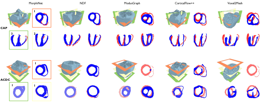
Figure 5: Surface reconstruction results on the CAP and ACDC datasets, depicting myocardium mesh slices in three views: 1) short-axis, 2) three-chamber, and 3) four-chamber. Note that the ACDC dataset provides no LAX image-view data. Those image-view planes are labelled as colour boxes and positioned against respective reconstructed models. In each boxed image view, the model’s cross-section (blue) is visualised in contrast with the manual segmentation (red). The RV myocardium segmentation in the ACDC dataset grows from RV epicardium, resulting in a 3 mm-thick myocardium free-wall segmentation.

Table 2: Evaluation results on CAP and ACDC datasets.

Dataset	Method	DiceSAX$\uparrow$	DiceLAX$\uparrow$	HdSAX$\downarrow$	HdLAX$\downarrow$	ASD$\downarrow$	AspR$\downarrow$	JacR$\uparrow$	NmF$\downarrow$	InFt$\downarrow$
	$\diamond$Voxel2Mesh	$0.39\left(0.09\right)$	$0.32\left(0.09\right)$	$10.63\left(3.08\right)$	$15.83\left(7.97\right)$	$6.14\left(2.00\right)$	$1.38\left(0.02\right)$	$0.71\left(0.01\right)$	$1.03\left(0.01\right)$	$0.32$
	$\diamond$CortFlow++	$0.38\left(0.08\right)$	$0.32\left(0.09\right)$	$7.90\left(2.05\right)$	$10.74\left(3.60\right)$	$3.44\left(1.05\right)$	$1.53\left(0.02\right)$	$0.64\left(0.01\right)$	$\textbf{0.04}\left(0.00\right)$	$0.68$
CAP	$\diamond$ModusGraph	$0.37\left(0.08\right)$	$0.31\left(0.09\right)$	$8.87\left(2.39\right)$	$14.59\left(5.83\right)$	$4.02\left(0.80\right)$	$\textbf{1.23}\left(0.00\right)$	$\textbf{0.81}\left(0.00\right)$	$\textbf{0.04}\left(0.00\right)$	0.07
	$\diamond$MorphiNet	$\textbf{0.59}\left(0.08\right)$	$\textbf{0.57}\left(0.08\right)$	$\textbf{3.63}\left(1.57\right)$	$\textbf{8.23}\left(7.13\right)$	$\textbf{3.06}\left(0.32\right)$	$1.58\left(0.07\right)$	$0.62\left(0.03\right)$	$\textbf{0.04}\left(0.00\right)$	$1.21$
	$\dagger$NDF	$0.60\left(0.11\right)$	$0.58\left(0.10\right)$	$3.19\left(2.82\right)$	$8.02\left(10.44\right)$	$2.14\left(0.27\right)$	$1.44\left(0.03\right)$	$0.68\left(0.02\right)$	$0.00\left(0.00\right)$	$122.54$
	$\diamond$Voxel2Mesh	$0.31\left(0.11\right)$	\	$18.27\left(7.33\right)$	\	$8.72\left(3.50\right)$	$1.42\left(0.04\right)$	$0.69\left(0.02\right)$	$1.03\left(0.01\right)$	$0.33$
	$\diamond$CortFlow++	$0.45\left(0.06\right)$	\	$7.21\left(2.30\right)$	\	$3.05\left(0.43\right)$	$1.54\left(0.03\right)$	$0.63\left(0.01\right)$	$\textbf{0.04}\left(0.00\right)$	$0.40$
ACDC	$\diamond$ModusGraph	$0.36\left(0.09\right)$	\	$11.30\left(2.54\right)$	\	$4.28\left(0.69\right)$	$\textbf{1.23}\left(0.00\right)$	$\textbf{0.81}\left(0.00\right)$	$\textbf{0.04}\left(0.00\right)$	0.08
	$\diamond$MorphiNet	$\textbf{0.68}\left(0.11\right)$	\	$\textbf{2.50}\left(1.69\right)$	\	$\textbf{3.19}\left(0.49\right)$	$1.61\left(0.09\right)$	$0.61\left(0.04\right)$	$\textbf{0.04}\left(0.00\right)$	$0.73$
	$\dagger$NDF	$0.74\left(0.07\right)$	\	$0.87\left(0.73\right)$	\	$2.37\left(0.56\right)$	$1.40\left(0.03\right)$	$0.71\left(0.01\right)$	$0.00\left(0.00\right)$	$123.66$

Notes: Dice and Hd are calculated based on pixels for SAX and LAX views. ASD is in mm. AspR, JacR, and NmF are dimensionless. InFt is in seconds. For ACDC, LAX scores are unavailable due to a lack of LAX data and denoted by ‘\’. Numbers represent average values and (standard deviation). The best scores of $\diamond$ explicit methods are in bold, and the $\dagger$ implicit method gives targeting scores.

4.3 Motion Tracking Evaluation

To assess MorphiNet’s capability in capturing cardiac motion, we conducted a comparative study with BiVModel [40], an established method for biventricular model registration. The evaluation focused on tracking cardiac motion from end-diastole (ED) to end-systole (ES). Fig. 6 visualizes the tracking results, showing model deformation across cardiac phases with displacement trajectories. Table 3 presents the quantitative assessment of motion tracking quality.

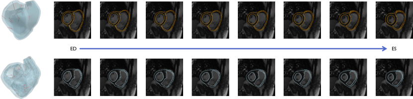
Figure 6: Models reconstructed per time frame from the ED to ES contrasting to the CMR images. The first row is BiVModel, and the second row is MorphiNet. The displacement trajectories of selected vertices are displayed as red lines overlaying on the left-most ED model. The trajectories of BiVModel are done by linear interpolation between the vertices of ED and ES models. The cross-section of each model is visualised against the CMR image at a respective time frame on the same axial view plane.

Table 3: Evaluation results of time-varying reconstruction for motion tracking on CAP cine CMR images.

Metric	BiVModel	MorphiNet
JacR$\uparrow$	0.73	0.62
AspR$\downarrow$	1.39	1.60
NmF$\downarrow$	0.02	0.04
Max Curvature$\downarrow$	0	129.96
Max Jerk$\downarrow$	0	0.03
LV EF (%)	43.99	24.87
RV EF (%)	37.64	25.06

Notes: Numbers without ‘Max’ represent average values; all values are dimensionless.

4.4 Ablation Studies

4.4.1 Segmentation Analysis

To evaluate the segmentation component of MorphiNet, we conducted a comparative analysis between the predicted and ground truth segmentations across CT and CMR data. For CT data, we examined the accuracy of the ResNet-restored segmentation, particularly focusing on the complementary slices near the basal and apex planes. We evaluated the segmentation accuracy for CMR data at both ED and ES phases before and after the ResNet restoration process. Table 4 compares these cardiac structures (LV, RV, and myocardium).

Table 4: Segmentation accuracy of CT and CMR data.

Metric	Region	CT	CMR-ED		CMR-ES
		after	before	after	before	after
	LV	0.92	0.90	0.88	0.86	0.81
Dice	MYO	0.81	0.71	0.63	0.72	0.63
	RV	0.92	0.88	0.87	0.84	0.83
	LV	1.20	1.60	2.69	2.14	4.14
Hd	MYO	1.23	2.05	3.15	2.14	3.95
	RV	1.17	2.47	3.60	2.71	3.70
	LV	-1.0	-7.68	3.39	11.19	30.64
Vol	MYO	1.0	-6.36	9.53	-9.20	28.26
Diff %	RV	0.0	-11.33	5.67	-5.89	16.78

Notes: CT scores are calculated using ResNet’s restored segmentation; CMR scores are calculated using dynUNet’s ED and ES data segmentation before and after ResNet’s restoration. Numbers represent average values; all values are dimensionless.

To visualize the impact of ResNet restoration, Fig. 7 shows representative examples of segmentation results before and after the ResNet processing. The comparison includes three key views of the cardiac structure, demonstrating the changes in predicted segmentation boundaries through restoration.

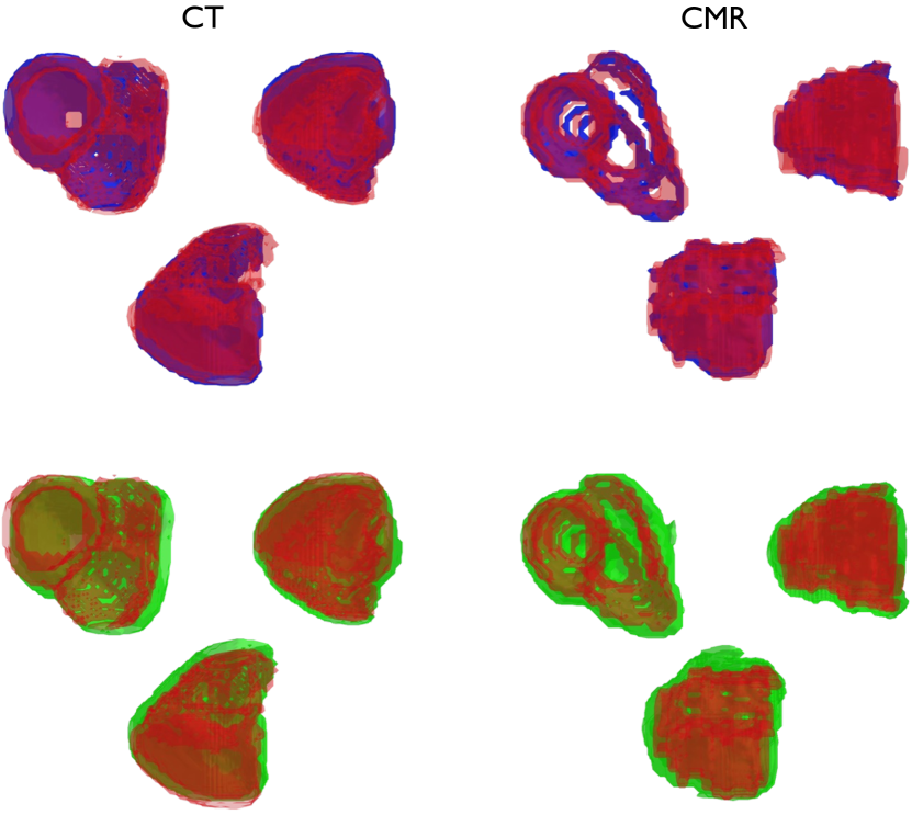
Figure 7: Visualisation of predicted segmentation changes before and after ResNet regarding shape and dimension. Contrasting the ground truth bi-ventricular myocardium segmentation (red) with a predicted segmentation before ResNet (first row in blue) and that after the ResNet restoration process (second row in green).

4.4.2 Deformation Strategy Comparison

We examined different mesh deformation approaches, comparing traditional Loop subdivision with our GSN-based method. Given the identical segmentation prediction from dynUNet, different approaches were applied to generate a model. \small1⃝ Base Model + Loop Subdivision used Loop subdivision on the template model unrelated to the segmentation; \small3⃝ Gradient Deformation follows the gradient-based mesh deformation (section 3.2) to adjust the template model against the segmentation; \small2⃝ Gradient Deformation + Loop Subdivision extend \small3⃝ by subdividing model’s surface using Loop subdivision; \small4⃝ Gradient Deformation + Single GSN and \small5⃝ Gradient Deformation + Double GSN use several GSN layers for subdividing models after the gradient-based mesh deformation. Table 5 presents the performance metrics for each strategy, evaluating both geometric accuracy and mesh quality.

Table 5: Evaluation results for different schemes applied to mesh deformation on CT data. \small1⃝ Base Model + Loop Subdivision, \small2⃝ Gradient Deformation + Loop Subdivision, \small3⃝ Gradient Deformation, \small4⃝ Gradient Deformation + Single GSN, \small5⃝ Gradient Deformation + Double GSN.

Scheme	Dice$\uparrow$	Hd$\downarrow$	ASD$\downarrow$	AspR$\downarrow$	JacR$\uparrow$	MnC$\uparrow$	NmF$\downarrow$
\small1⃝	0.55	4.24	2.91	1.34	0.76	0.76	0.04
\small2⃝	0.68	3.27	2.63	1.37	0.73	0.77	0.04
\small3⃝	0.73	2.62	13.22	1.45	0.67	0.69	0.18
\small4⃝	0.73	2.61	4.76	1.40	0.70	0.76	0.09
\small5⃝	0.73	2.55	2.84	1.49	0.66	0.77	0.04

Notes: Dice and Hd are calculated based on pixels; ASD is in mm; AspR, JacR, MnC, and NmF are dimensionless. Numbers represent average values. Best scores are in bold.

4.4.3 Training Data Impact

The influence of CT training data volume was investigated using different data ratios. Fig. 8 shows the learning curves under various training data configurations. MorphiNet was trained on a ratio of CT data taken after being randomly scattered five times. The Dice score is the average of five test scores on CMR data, and the Dice loss is recorded when the highest Dice score is achieved. When no CT training data was used, ground truth CMR segmentation and images were used to train all MorphiNet components. Fig. 9 illustrates the convergence behaviour during training under different CT data ratios. We record the loss convergence during training GSN since a more observable difference exists against different CT data ratios than training other MorphiNet components.

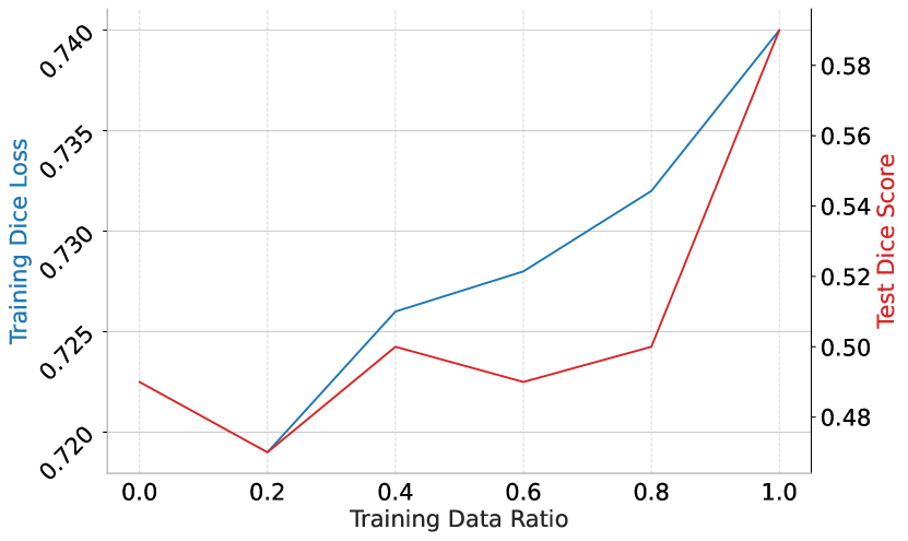
Figure 8: Learning curve showing MorphiNet’s performance with different volumes of CT training data. The curve includes the training Dice loss evaluated with CT data and the test Dice score evaluated on CMR data.

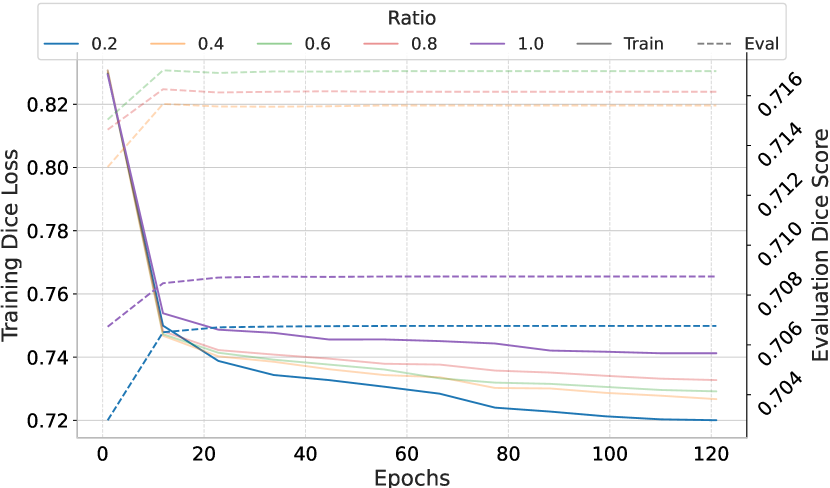
Figure 9: Training convergence analysis (during GSN training) showing the contrast between training Dice loss and evaluation Dice score during MorphiNet training with different CT training data ratios.

5 Discussion

MorphiNet demonstrates significant advantages in cardiac mesh reconstruction. The method achieves Dice scores of 0.73 on CT data and 0.59 on CMR data, representing approximately 40% improvement over previous explicit reconstruction methods like ModusGraph. This improved accuracy stems from the gradient field-guided deformation process, which enables better preservation of anatomical structures.

A fundamental challenge lies in the control of mesh deformation. While MorphiNet’s explicit vertex displacement approach offers better topology control, it provides less precise control over local deformations than implicit methods like NDF’s pixel-wise approach. This limitation is particularly evident in predicting myocardium wall thickness, especially for the thin ($\approx$3 mm) RV myocardium. The average surface distance of explicit methods (2.84 mm for MorphiNet) remains larger than that of NDF (0.89 mm), primarily due to surface discrepancies near the valves. These discrepancies result from alignment challenges during gradient-field deformation, where valve positions cannot be precisely determined without accurate localization of chamber intersections.

Despite these challenges, MorphiNet’s explicit mesh representation offers distinct advantages for computational analysis. The method maintains fixed triangular face topology and consistent vertex count (from 388 vertices to 6,238 after two GSN layers), enabling straightforward point correspondence tracking between time frames. This feature is particularly valuable for motion analysis and dynamic studies, making MorphiNet more suitable than implicit methods for comprehensive cardiac assessment. The computational efficiency is noteworthy, with an inference time of 1.34s compared to NDF’s 122.64s, suggesting potential for real-time applications.

The anatomical fidelity of MorphiNet presents interesting trade-offs. While the method preserves detailed structures like papillary muscles from the dynUNet segmentation, this preservation affects septum wall thickness prediction. Our analysis systematically reveals lower ejection fraction predictions (LV: 24.87%, RV: 25.06%) than established methods like BiVModel (LV: 43.99%, RV: 37.64%). This discrepancy stems from volume prediction bias, where ResNet’s complementary segmentation shows systematic overestimation (Fig. 7), particularly evident in end-systolic cases with volume differences up to 30.64% for LV.

The mesh quality analysis reveals complex relationships between anatomical fidelity and mesh quality. Adding GSN layers improves surface accuracy but can affect mesh quality metrics. MorphiNet achieves acceptable quality scores (AspR: 1.49, JacR: 0.66) after Laplacian smoothing, though slightly lower than some baseline methods. The trade-off between mesh refinement and quality suggests the need for more sophisticated regularization approaches in future developments.

The CT training data ratio analysis reveals concerns over ResNet’s systematic overestimation. MorphiNet exhibits rapid overfitting during GSN training regardless of data volume, with performance metrics on CMR reconstruction improving as more CT data is added. While increasing CT training data might seem beneficial, two key constraints remain: maintaining balance with available CMR data for effective cross-modality adaptation and anatomical differences in CT and CMR data that reinforce existing biases in ResNet’s complementary segmentation.

For future improvements, the ResNet’s restoration process could be enhanced with volume-preserving constraints and improved cross-modality adaptation strategies. The valve positions can be determined with the atrioventricular valve plane or the valve plane between ventricles and the major outflow vessels derived from multi-chamber segmentations from dynUNets. Adaptive GSN architectures could use diffeomorphic regularisation that balances refinement quality with mesh properties. The method’s combination of accuracy, efficiency, and topology preservation makes it promising for research and clinical applications, though careful consideration of its limitations remains important for specific use cases.

6 Conclusion

In this paper, we address the challenges in heart model reconstruction and modelling due to the anisotropic characteristics of CMR imaging while acknowledging the complementary anatomical insights offered by CT. We propose MorphiNet, a latent representation network that predicts a continuous gradient field and adaptively adjusts and refines the mesh with our GSN structure in a patient-specific manner. Compared with state-of-the-art methods, empirical validation on CMR and CT datasets substantiates MorphiNet’s performance in capturing complex heart anatomical entities, demonstrating its potential to generate high-fidelity heart mesh models .

References

- [1] R. Chabiniok, V. Y. Wang, M. Hadjicharalambous, L. Asner, J. Lee, M. Sermesant, E. Kuhl, A. A. Young, P. Moireau, M. P. Nash, et al., “Multiphysics and multiscale modelling, data–model fusion and integration of organ physiology in the clinic: ventricular cardiac mechanics,” Interface focus, vol. 6, no. 2, p. 20150083, 2016.
- [2] A. Nasopoulou, A. Shetty, J. Lee, D. Nordsletten, C. A. Rinaldi, P. Lamata, and S. Niederer, “Improved identifiability of myocardial material parameters by an energy-based cost function,” Biomechanics and modeling in mechanobiology, vol. 16, pp. 971–988, 6 2017.
- [3] B. Villard, E. Zacur, E. Dall’Armellina, and V. Grau, “Correction of slice misalignment in multi-breath-hold cardiac mri scans,” in Statistical Atlases and Computational Models of the Heart. Imaging and Modelling Challenges: 7th International Workshop, STACOM 2016, Held in Conjunction with MICCAI 2016, Athens, Greece, October 17, 2016, Revised Selected Papers 7, pp. 30–38, Springer, 2017.
- [4] G. Tarroni, O. Oktay, M. Sinclair, W. Bai, A. Schuh, H. Suzuki, A. de Marvao, D. O’Regan, S. Cook, and D. Rueckert, “A comprehensive approach for learning-based fully-automated inter-slice motion correction for short-axis cine cardiac mr image stacks,” in Medical Image Computing and Computer Assisted Intervention–MICCAI 2018: 21st International Conference, Granada, Spain, September 16-20, 2018, Proceedings, Part I, pp. 268–276, Springer, 2018.
- [5] Y. Xia, N. Ravikumar, J. P. Greenwood, S. Neubauer, S. E. Petersen, and A. F. Frangi, “Super-resolution of cardiac mr cine imaging using conditional gans and unsupervised transfer learning,” Medical Image Analysis, vol. 71, p. 102037, 2021.
- [6] S. Gong, W. Lu, J. Xie, X. Zhang, S. Zhang, and Q. Dou, “Robust cardiac mri segmentation with data-centric models to improve performance via intensive pre-training and augmentation,” in International Workshop on Statistical Atlases and Computational Models of the Heart, pp. 494–504, Springer, 2022.
- [7] T. J. Hughes, The finite element method: linear static and dynamic finite element analysis. Courier Corporation, 2012.
- [8] S. Osher, R. Fedkiw, and K. Piechor, “Level set methods and dynamic implicit surfaces,” Appl. Mech. Rev., vol. 57, no. 3, pp. B15–B15, 2004.
- [9] X. Chen, N. Ravikumar, Y. Xia, R. Attar, A. Diaz-Pinto, S. K. Piechnik, S. Neubauer, S. E. Petersen, and A. F. Frangi, “Shape registration with learned deformations for 3d shape reconstruction from sparse and incomplete point clouds,” Medical Image Analysis, vol. 74, p. 102228, 2021.
- [10] U. Wickramasinghe, E. Remelli, G. Knott, and P. Fua, “Voxel2mesh: 3d mesh model generation from volumetric data,” in Medical Image Computing and Computer Assisted Intervention–MICCAI 2020: 23rd International Conference, Lima, Peru, October 4–8, 2020, Proceedings, Part IV 23, pp. 299–308, Springer, 2020.
- [11] F. Kong, N. Wilson, and S. Shadden, “A deep-learning approach for direct whole-heart mesh reconstruction,” Medical image analysis, vol. 74, p. 102222, 2021.
- [12] Y. Deng, H. Xu, S. Rodrigo, S. E. Williams, M. C. Williams, S. A. Niederer, K. Pushparajah, and A. Young, “Modusgraph: Automated 3d and 4d mesh model reconstruction from cine cmr with improved accuracy and efficiency,” in International Conference on Medical Image Computing and Computer-Assisted Intervention, pp. 173–183, Springer, 2023.
- [13] H. Fan, H. Su, and L. J. Guibas, “A point set generation network for 3d object reconstruction from a single image,” in Proceedings of the IEEE conference on computer vision and pattern recognition, pp. 605–613, 2017.
- [14] Y. Deng, Y. Xu, L. Qian, A. Nasopoulou, S. Williams, M. Williams, S. Niederer, K. Pushprajah, and A. Young, “Adaptive bi-ventricle surface reconstruction from cardiovascular imaging,” in International Workshop on Shape in Medical Imaging, pp. 112–122, Springer, 2024.
- [15] A. A. Young, B. R. Cowan, S. F. Thrupp, W. J. Hedley, and L. J. Dell’Italia, “Left ventricular mass and volume: fast calculation with guide-point modeling on mr images,” Radiology, vol. 216, no. 2, pp. 597–602, 2000.
- [16] A. F. Frangi, D. Rueckert, J. A. Schnabel, and W. J. Niessen, “Automatic construction of multiple-object three-dimensional statistical shape models: Application to cardiac modeling,” IEEE transactions on medical imaging, vol. 21, no. 9, pp. 1151–1166, 2002.
- [17] D. Perperidis, R. Mohiaddin, and D. Rueckert, “Construction of a 4d statistical atlas of the cardiac anatomy and its use in classification,” in Medical Image Computing and Computer-Assisted Intervention–MICCAI 2005: 8th International Conference, Palm Springs, CA, USA, October 26-29, 2005, Proceedings, Part II 8, pp. 402–410, Springer, 2005.
- [18] A. A. Young and A. F. Frangi, “Computational cardiac atlases: from patient to population and back,” Experimental physiology, vol. 94, no. 5, pp. 578–596, 2009.
- [19] P. Medrano-Gracia, B. R. Cowan, D. A. Bluemke, J. P. Finn, J. A. Lima, A. Suinesiaputra, and A. A. Young, “Large scale left ventricular shape atlas using automated model fitting to contours,” in Functional Imaging and Modeling of the Heart: 7th International Conference, FIMH 2013, London, UK, June 20-22, 2013. Proceedings 7, pp. 433–441, Springer, 2013.
- [20] W. Bai, W. Shi, A. de Marvao, T. J. Dawes, D. P. O’Regan, S. A. Cook, and D. Rueckert, “A bi-ventricular cardiac atlas built from 1000+ high resolution mr images of healthy subjects and an analysis of shape and motion,” Medical image analysis, vol. 26, no. 1, pp. 133–145, 2015.
- [21] E. Puyol-Anton, M. Sinclair, B. Gerber, M. S. Amzulescu, H. Langet, M. De Craene, P. Aljabar, P. Piro, and A. P. King, “A multimodal spatiotemporal cardiac motion atlas from mr and ultrasound data,” Medical image analysis, vol. 40, pp. 96–110, 2017.
- [22] A. Suinesiaputra, P. Ablin, X. Alba, M. Alessandrini, J. Allen, W. Bai, S. Cimen, P. Claes, B. R. Cowan, J. D’hooge, et al., “Statistical shape modeling of the left ventricle: myocardial infarct classification challenge,” IEEE journal of biomedical and health informatics, vol. 22, no. 2, pp. 503–515, 2017.
- [23] K. Gilbert, C. Mauger, A. A. Young, and A. Suinesiaputra, “Artificial intelligence in cardiac imaging with statistical atlases of cardiac anatomy,” Frontiers in Cardiovascular Medicine, vol. 7, p. 102, 2020.
- [24] M. Marciniak, A. W. van Deutekom, L. Toemen, A. J. Lewandowski, R. Gaillard, A. A. Young, V. W. Jaddoe, and P. Lamata, “A three-dimensional atlas of child’s cardiac anatomy and the unique morphological alterations associated with obesity,” European Heart Journal-Cardiovascular Imaging, vol. 23, no. 12, pp. 1645–1653, 2022.
- [25] S. Govil, B. T. Crabb, Y. Deng, L. Dal Toso, E. Puyol-Antón, K. Pushparajah, S. Hegde, J. C. Perry, J. H. Omens, A. Hsiao, et al., “A deep learning approach for fully automated cardiac shape modeling in tetralogy of fallot,” Journal of Cardiovascular Magnetic Resonance, vol. 25, no. 1, p. 15, 2023.
- [26] H. Xu, E. Zacur, J. E. Schneider, and V. Grau, “Ventricle surface reconstruction from cardiac mr slices using deep learning,” in Functional Imaging and Modeling of the Heart: 10th International Conference, FIMH 2019, Bordeaux, France, June 6–8, 2019, Proceedings 10, pp. 342–351, Springer, 2019.
- [27] M. Beetz, A. Banerjee, J. Ossenberg-Engels, and V. Grau, “Multi-class point cloud completion networks for 3d cardiac anatomy reconstruction from cine magnetic resonance images,” Medical Image Analysis, vol. 90, p. 102975, 2023.
- [28] Q. Meng, W. Bai, D. P. O’Regan, and D. Rueckert, “Deepmesh: Mesh-based cardiac motion tracking using deep learning,” IEEE transactions on medical imaging, 2023.
- [29] X. Yuan, C. Liu, and Y. Wang, “4d myocardium reconstruction with decoupled motion and shape model,” in Proceedings of the IEEE/CVF International Conference on Computer Vision, pp. 21252–21262, 2023.
- [30] J. Verhülsdonk, T. Grandits, F. S. Costabal, T. Pinetz, R. Krause, A. Auricchio, G. Haase, S. Pezzuto, and A. Effland, “Shape of my heart: Cardiac models through learned signed distance functions,” arXiv preprint arXiv:2308.16568, 2023.
- [31] N. Stolt-Ansó, J. McGinnis, J. Pan, K. Hammernik, and D. Rueckert, “Nisf: Neural implicit segmentation functions,” in International Conference on Medical Image Computing and Computer-Assisted Intervention, pp. 734–744, Springer, 2023.
- [32] M. Muffoletto, H. Xu, Y. Xu, S. E. Williams, M. C. Williams, K. P. Kunze, R. Neji, S. A. Niederer, D. Rueckert, and A. A. Young, “Neural implicit functions for 3d shape reconstruction from standard cardiovascular magnetic resonance views,” in International Workshop on Statistical Atlases and Computational Models of the Heart, pp. 130–139, Springer, 2023.
- [33] F. Kong, S. Stocker, P. S. Choi, M. Ma, D. B. Ennis, and A. Marsden, “Sdf4chd: Generative modeling of cardiac anatomies with congenital heart defects,” Medical Image Analysis, p. 103293, 2024.
- [34] M. Ranzini, L. Fidon, S. Ourselin, M. Modat, and T. Vercauteren, “Monaifbs: Monai-based fetal brain mri deep learning segmentation,” arXiv preprint arXiv:2103.13314, 2021.
- [35] M. MONAI Consortium et al., “Monai: Medical open network for ai,” Online at https://doi. org/10.5281/zenodo, vol. 5525502, 2020.
- [36] F. Isensee, P. F. Jaeger, S. A. Kohl, J. Petersen, and K. H. Maier-Hein, “nnu-net: a self-configuring method for deep learning-based biomedical image segmentation,” Nature methods, vol. 18, no. 2, pp. 203–211, 2021.
- [37] A. Myronenko, “3d mri brain tumor segmentation using autoencoder regularization,” in Brainlesion: Glioma, Multiple Sclerosis, Stroke and Traumatic Brain Injuries: 4th International Workshop, BrainLes 2018, Held in Conjunction with MICCAI 2018, Granada, Spain, September 16, 2018, Revised Selected Papers, Part II 4, pp. 311–320, Springer, 2019.
- [38] M. J. Cardoso, W. Li, R. Brown, N. Ma, E. Kerfoot, Y. Wang, B. Murrey, A. Myronenko, C. Zhao, D. Yang, et al., “Monai: An open-source framework for deep learning in healthcare,” arXiv preprint arXiv:2211.02701, 2022.
- [39] C. H. Sudre, W. Li, T. Vercauteren, S. Ourselin, and M. Jorge Cardoso, “Generalised dice overlap as a deep learning loss function for highly unbalanced segmentations,” in Deep Learning in Medical Image Analysis and Multimodal Learning for Clinical Decision Support: Third International Workshop, DLMIA 2017, and 7th International Workshop, ML-CDS 2017, Held in Conjunction with MICCAI 2017, Québec City, QC, Canada, September 14, Proceedings 3, pp. 240–248, Springer, 2017.
- [40] C. Mauger, K. Gilbert, A. Suinesiaputra, B. Pontré, J. Omens, A. McCulloch, and A. Young, “An Iterative Diffeomorphic Algorithm for Registration of Subdivision Surfaces: Application to Congenital Heart Disease,” in 2018 40th Annual International Conference of the IEEE Engineering in Medicine and Biology Society (EMBC), pp. 596–599, July 2018.
- [41] A. Paszke, S. Gross, F. Massa, A. Lerer, J. Bradbury, G. Chanan, T. Killeen, Z. Lin, N. Gimelshein, L. Antiga, et al., “Pytorch: An imperative style, high-performance deep learning library,” Advances in neural information processing systems, vol. 32, 2019.
- [42] C. Loop, “Smooth subdivision surfaces based on triangles,” 1987.
- [43] D. Zorin, P. Schröder, and W. Sweldens, “Interpolating subdivision for meshes with arbitrary topology,” in Proceedings of the 23rd annual conference on Computer graphics and interactive techniques, pp. 189–192, 1996.
- [44] M. Desbrun, M. Meyer, P. Schröder, and A. H. Barr, “Implicit fairing of irregular meshes using diffusion and curvature flow,” in Proceedings of the 26th annual conference on Computer graphics and interactive techniques, pp. 317–324, 1999.
- [45] N. Ravi, J. Reizenstein, D. Novotny, T. Gordon, W.-Y. Lo, J. Johnson, and G. Gkioxari, “Accelerating 3d deep learning with pytorch3d,” arXiv preprint arXiv:2007.08501, 2020.
- [46] S.-H. Investigators, “Coronary ct angiography and 5-year risk of myocardial infarction,” New England Journal of Medicine, vol. 379, no. 10, pp. 924–933, 2018.
- [47] X. Zhuang, “Multivariate mixture model for myocardial segmentation combining multi-source images,” IEEE transactions on pattern analysis and machine intelligence, vol. 41, no. 12, pp. 2933–2946, 2018.
- [48] O. Bernard, A. Lalande, C. Zotti, F. Cervenansky, X. Yang, P.-A. Heng, I. Cetin, K. Lekadir, O. Camara, M. A. G. Ballester, et al., “Deep learning techniques for automatic mri cardiac multi-structures segmentation and diagnosis: is the problem solved?,” IEEE transactions on medical imaging, vol. 37, no. 11, pp. 2514–2525, 2018.
- [49] I. Loshchilov, “Decoupled weight decay regularization,” arXiv preprint arXiv:1711.05101, 2017.
- [50] R. Santa Cruz, L. Lebrat, D. Fu, P. Bourgeat, J. Fripp, C. Fookes, and O. Salvado, “Corticalflow++: Boosting cortical surface reconstruction accuracy, regularity, and interoperability,” in International Conference on Medical Image Computing and Computer-Assisted Intervention, pp. 496–505, Springer, 2022.
- [51] S. Sun, K. Han, D. Kong, H. Tang, X. Yan, and X. Xie, “Topology-preserving shape reconstruction and registration via neural diffeomorphic flow,” in Proceedings of the IEEE/CVF Conference on Computer Vision and Pattern Recognition, pp. 20845–20855, 2022.
- [52] A. A. Taha and A. Hanbury, “Metrics for evaluating 3d medical image segmentation: analysis, selection, and tool,” BMC medical imaging, vol. 15, pp. 1–28, 2015.
- [53] H. S. Kim, S. B. Park, S. S. Lo, J. I. Monroe, and J. W. Sohn, “Bidirectional local distance measure for comparing segmentations,” Medical physics, vol. 39, no. 11, pp. 6779–6790, 2012.