Distributed Estimation with Quantized Measurements and Communication over Markovian Switching Topologies

Ying Wang wangying96@amss.ac.cn    Jian Guo j.guo@amss.ac.cn    Yanlong Zhao ylzhao@amss.ac.cn    Ji-Feng Zhang jif@iss.ac.cn Key Laboratory of Systems and Control, Academy of Mathematics and Systems Science, Chinese Academy of Sciences, Beijing 100190, P. R. China. Division of Decision and Control Systems, KTH Royal Institute of Technology, Stockholm 11428, Sweden. School of Mathematical Sciences, University of Chinese Academy of Sciences, Beijing 100049, P. R. China. School of Automation and Electrical Engineering, Zhongyuan University of Technology, Zhengzhou 450007, P. R. China
Abstract

This paper addresses distributed parameter estimation in stochastic dynamic systems with quantized measurements, constrained by quantized communication and Markovian switching directed topologies. To enable accurate recovery of the original signal from quantized communication signal, a persistent excitation-compliant linear compression encoding method is introduced. Leveraging this encoding, this paper proposes an estimation-fusion type quantized distributed identification algorithm under a stochastic approximation framework. The algorithm operates in two phases: first, it estimates neighboring estimates using quantized communication information, then it creates a fusion estimate by combining these estimates through a consensus-based distributed stochastic approximation approach. To tackle the difficulty caused by the coupling between these two estimates, two combined Lyapunov functions are constructed to analyze the convergence performance. Specifically, the mean-square convergence of the estimates is established under a conditional expectation-type cooperative excitation condition and the union topology containing a spanning tree. Besides, the convergence rate is derived to match the step size’s order under suitable step-size coefficients. Furthermore, the impact of communication uncertainties including stochastic communication noise and Markov-switching rate is analyzed on the convergence rate. A numerical example illustrates the theoretical findings and highlights the joint effect of sensors under quantized communication.

keywords:
Distributed estimation, quantized measurements, quantized communication, Markovian switching topologies, stochastic approximation
thanks: The work is supported by National Natural Science Foundation of China under Grants 62025306, 62433020, 62303452, T2293770 and 62473040, and CAS Project for Young Scientists in Basic Research under Grant YSBR-008. The material in this paper was not presented at any conference. Corresponding author: Yanlong Zhao.

, , ,

1 Introduction

1.1 Background and Motivations

Wireless sensor networks (WSNs) are extensively used in fields such as environmental monitoring, intelligent transportation, and smart agriculture due to their easy deployment, flexibility, low power consumption, high accuracy, and reliability (Akyildiz et al., 2002; Taj and Cavallaro, 2011; Rawat et al., 2014; Ge et al., 2020). Distributed parameter estimation over sensor networks is a critical theoretical issue in WSNs research and has garnered significant academic attention (Dimakis et al., 2010; Bianchi et al., 2013; Mateos and Giannakis, 2012). Various effective distributed estimation algorithms have been developed, including distributed stochastic approximation algorithms (Zhang and Zhang, 2012; Lei and Chen, 2020), distributed stochastic gradient algorithms (Gan and Liu, 2024; Swenson et al., 2020), and distributed least squares algorithms (Takahashi et al., 2010; Xie et al., 2021). These distributed approaches only rely on partial information and local data exchange due to collaboration constraints caused by the sensing and communication limitations of individual sensors. However, it is important to note that these algorithms generally assume both accurate communication and precise measurements.

Actually, WSNs consists of numerous spatially distributed sensor nodes, each powered by batteries and equipped with sensing, communication, and computational capabilities. Consequently, WSNs face significant energy and communication constraints due to limited battery life in addition to the inherent collaboration limitations (Akyildiz et al., 2002; Rawat et al., 2014). Key constraints include:

  • Energy constraints (Han et al., 2023a, b): Limited sensing and measurement ranges, restricted processing capabilities, small memory, and more.

  • Communication constraints (Ge et al., 2020): Short communication bandwidth, time-varying network topology, network link failures, and more.

It is well-known that both data transmission and measurement consume more energy than local data processing, with communication being the most energy-intensive of the three (Pottie and Kaiser, 2000). Therefore, reducing the bandwidth required for data transmission and the precision of measurement data can significantly extend battery life. Consequently, designing distributed adaptive estimation algorithms that can cooperatively estimate unknown parameters based on quantized transmitted data and quantized measurement data has become an increasingly important research focus.

1.2 Related literature

Quantized data refers to data where only the set it belongs to is known, without precise knowledge of exact values, i.e., data with finite precision or bits (Wang et al., 2003). The existing works on distributed estimation with quantized data generally falls into two categories:

Distributed estimation with quantized measurements: Here, each sensor has quantized measurements but can communicate accurately with its neighbors (Ding et al., 2017; Wang and Zhang, 2019; Wang et al., 2021; Fu et al., 2022; Han et al., 2023a, b). For example, Fu et al. (2022) investigated distributed estimation with binary-valued measurements in time-varying networks, proposing a distributed stochastic approximation algorithm with extended truncation and proving its almost sure convergence under strictly stationary signals. Besides, Wang et al. (2021) developed a Quasi-Newton type projection algorithm with a time-varying projection operator and a diffusion strategy under binary measurements and an undirected, connected topology, achieving almost sure convergence without relying on signal periodicity, independence, or stationarity.

Distributed estimation with quantized communication: In this approach, sensors have accurate measurements but can only communicate with neighbors through quantized channels (Kar et al., 2012; Zhu et al., 2015, 2017, 2018; Li et al., 2023). For instance, Kar et al. (2012) proposed a consensus+innovations distributed algorithm based on stochastic approximation idea and probabilistic quantizer-based communication, showing almost sure convergence in undirected and connected topologies. Additionally, Zhu et al. (2015) and Zhu et al. (2018) introduced running average distributed estimation algorithms within the consensus+innovation framework, using probabilistic quantized communication with only one measurement per sensor.

While these approaches are insightful, the first class addresses quantized measurement alone, without considering the complexity and energy demands of quantized communication. The second class, meanwhile, overlooks the irreversible loss of information caused by quantized measurements. Furthermore, both approaches fail to account for the effects of unreliable communication networks, such as time-varying topologies and stochastic communication noise. The goal of this paper, therefore, is to develop a distributed estimation algorithm that integrates both quantized measurements and quantized communication under Markov-switching topologies and stochastic communication noise, thereby reducing communication bandwidth and measurement precision requirements to extend sensor battery life substantially.

1.3 Main contribution

This paper investigates the distributed parameter estimation problem with both quantized measurements and quantized communication in the presence of Markov-switching directed topologies and stochastic communication noise. The primary contributions of this study, in contrast to previous work, are as follows:

  • Problem aspect: This work is the first to address distributed parameter estimation with both quantized measurements and quantized communication, while also accounting for communication uncertainties such as Markov-switching topologies and stochastic communication noise (Kar et al., 2012; Zhu et al., 2015, 2018; Li et al., 2023; Ding et al., 2017; Wang et al., 2021; Fu et al., 2022). Additionally, it achieves one-bit communication through a linear compression encoding method, significantly reducing communication costs compared to prior methods (Kar et al., 2012; Zhu et al., 2015, 2018; Li et al., 2023).

  • Algorithm aspect: An estimation-fusion type quantized distributed identification (EFTQDI) algorithm is proposed to handle quantized measurements and quantized communication. To counteract the information reduction and nonlinearity from quantized communication, the estimate of neighboring estimate is designed using a stochastic approximation approach. Notably, a linear communication encoding method satisfying persistent excitation condition (Wang et al., 2022) is developed, ensuring that the original information can be reconstructed from one-bit transmitted data. Then, the algorithm creates a fusion estimate by using stochastic approximation idea through a combination of these estimates and a consensus strategy.

  • Result aspect: By constructing two Lyapunov functions to analyse the coupling relationship of two estimates, this paper establishes the mean-square convergence of both the fusion estimate and the estimate of neighboring estimate under a conditional expectation-type cooperative excitation condition, which is more general than typical cooperative excitation conditions (Kar et al., 2012; Zhang and Zhang, 2012; Fu et al., 2022). Additionally, the mean-square convergence rate of the EFTQDI algorithm is shown to match the order of the step size. This work further analyzes the impact of communication uncertainties, such as stochastic communication noise and Markov-switching rates, on the convergence rate.

The remainder of this paper is organized as follows. Section 2 introduces graph preliminaries and problem formulation. Section 3 presents the proposed algorithm, while Section 4 demonstrates its convergence properties. Proofs of the main results are provided in Section 5. Section 6 includes a numerical example to illustrate the main findings, and Section 7 concludes the paper and discusses potential future work.

Notations. This paper uses $x=[x_{1},\ldots,x_{n}]^{T}\in\mathbb{R}^{n}$ and $A\in\mathbb{R}^{m\times n}$ to denote $n$-dimensional vector and $m\times n$-dimensional real matrix respectively. Moreover, we denote $\|x\|=\sum_{i=1}^{n}{x_{i}^{2}}$ and $\|A\|=\left(\lambda_{\max}(A^{T}A)\right)^{\frac{1}{2}}$ as the Euclidean norm of vector and matrix respectively, where the notation $T$ denotes the transpose operator and $\lambda_{\max}(\cdot)$ denotes the largest eigenvalue of the matrix. Correspondingly, we use $\lambda_{\min}(\cdot)$ to denote the smallest eigenvalue of the matrix. The function $I_{\{\cdot\}}$ denotes the indicator function, whose value is 1 if its argument is true, and 0, otherwise. Let $A$ and $B$ be two symmetric matrices, then $A\geq B$ means that $A-B$ is a positive semi-definite matrix. The Kronecker product of two matrices $A=\{a_{ij}\}\in\mathbb{R}^{m\times n}$ and $B\in\mathbb{R}^{p\times q}$ is defined as

$$A\otimes B=\left(\begin{array}[]{ccc}a_{11}B&\cdots&a_{1n}B\\ \vdots&\ddots&\vdots\\ a_{m1}B&\cdots&a_{mn}B\\ \end{array}\right)\in\mathbb{R}^{mp\times nq}.$$

2 Problem formulation

2.1 Graph Preliminaries

In order to describe the relationship between sensor nodes, a sequence of time-varying digraphs $\mathcal{G}_{k}=(\mathcal{V},\mathcal{E}_{k},\mathcal{A}_{k})$ are introduced here, where $\mathcal{V}=\{1,2,\ldots,m\}$ is the set of nodes, and the node $i\in\mathcal{V}$ represent the sensor node $i$. $\mathcal{E}_{k}\subseteq\mathcal{V}\times\mathcal{V}$ is the edge set which is used to describe the communication between agents at time $k$, and a directed edge $(i,j)\in\mathcal{E}_{k}$ if and only if there is a communication link from $i$ to $j$ at time $k$. $\mathcal{A}_{k}=\{a_{ij,k}\}\in\mathbb{R}^{m\times m}$ is the adjacency matrix of $\mathcal{G}_{k}$. The elements of the matrix $\mathcal{A}_{k}$ satisfy: $0<a_{ij,k}<1$ if and only if $(j,i)\in\mathcal{E}_{k}$, otherwise $a_{ij,k}=0$. The set of the neighbors of agent $i$ at time $k$ is denoted as $\mathcal{N}_{i,k}=\{j\in\mathcal{V}|(j,i)\in\mathcal{E}_{k}\}$ and each agent can only exchange information with its neighbors. The Laplacian matrix of $\mathcal{G}_{k}$ is defined as $\mathcal{L}_{k}=\operatorname{diag}\{\sum_{j=1}^{m}a_{1j,k},\sum_{j=1}^{m}a_{2j,k},\ldots,\sum_{j=1}^{m}a_{mj,k}\}-\mathcal{A}_{k}$.

The dynamic changes of the communication topology digraph $\mathcal{G}_{k}$ is described with a Markovian chain $\{m_{k},k=1,2,\ldots\}$ with a finite state space $\mathcal{S}=\{1,2,\ldots,s\}$ and transition probability $p_{uv}=\mathbb{P}\left(m_{k+1}=v\mid m_{k}=u\right)$. Then the corresponding communication topology digraph set is $\{\mathcal{G}^{(1)},\ldots,\mathcal{G}^{(s)}\}$, where $\mathcal{G}^{(u)}=(\mathcal{V},\mathcal{E}^{(u)},\mathcal{A}^{(u)})$ is a digraph, $\mathcal{E}^{(u)}$, $\mathcal{A}^{(u)}=\{a_{ij}^{(u)}\}$ and $\mathcal{L}^{(u)}$ are the corresponding edge set, adjacency matrix and Laplacian matrix for $u\in S$. We say $m_{k}=u$ if and only if $\mathcal{G}_{k}=\mathcal{G}^{(u)}$. The union topology of $\mathcal{G}^{(1)},\ldots,\mathcal{G}^{(s)}$ is denoted by $\mathcal{G}_{\mathcal{C}}=\left(\mathcal{V},\mathcal{E}_{\mathcal{C}},\mathcal{A}_{\mathcal{C}}\right)$, where $\mathcal{E}_{\mathcal{C}}=\bigcup_{u=1}^{s}\mathcal{E}^{(u)}$ and $\mathcal{A}_{\mathcal{C}}=\left\{{a}_{ij}^{\mathcal{C}}\right\}$. A directed tree is a digraph, where each node except the root has exactly one parent node. A spanning tree of $\mathcal{G}_{\mathcal{C}}$ is a directed tree whose node set is $\mathcal{V}$ and whose edge set is a subset of $\mathcal{E}_{\mathcal{C}}$. Besides, $\mathcal{G}_{\mathcal{C}}$ is called a balanced digraph if $\sum_{j=1}^{m}a_{ij}^{\mathcal{C}}=\sum_{j=1}^{m}a_{ji}^{\mathcal{C}}$ for all $i\in\mathcal{V}$. $\mathcal{G}_{\mathcal{C}}$ is called an undirected graph, if $\mathcal{A}_{\mathcal{C}}$ is symmetric. The mirror graph $\hat{\mathcal{G}}_{\mathcal{C}}$ of the digraph $\mathcal{G}_{\mathcal{C}}$ is an undirected graph, denoted by $\hat{\mathcal{G}}_{\mathcal{C}}=(\mathcal{V},\hat{\mathcal{E}}_{\mathcal{C}},\hat{\mathcal{A}}_{\mathcal{C}})$ with $\hat{\mathcal{A}}_{\mathcal{C}}=\{\hat{a}_{ij}^{\mathcal{C}}\}$, $\hat{a}_{ij}^{\mathcal{C}}=\hat{a}_{ji}^{\mathcal{C}}=({a}_{ij}^{\mathcal{C}}+{a}_{ji}^{\mathcal{C}})/2$.

Remark 2.1.

The switching topology described by the above Markovian chain can effectively model link failures or losses between the channels of a WSN (Zhang and Zhang, 2012). Actually, the number of failure-prone links $m_{f}$ is finite with $m_{f}\leq m(m-1)$. It implies that the total possible configurations of the WSN with link failures is also finite, with an upper bound of $2^{m_{f}}$. We use the Markovian chain $m_{k}$ to represent these link failures at time $k$, where $m_{k}$ is an $m_{f}$-dimensional vector with each component taking a value of 00 or $1$ to indicate whether a link is absent or present. In this case, the state space of the Markovian chain $m_{k}$ is finite and denoted by $\mathcal{S}$. The corresponding topology are represented by $\{\mathcal{G}^{(1)},\ldots,\mathcal{G}^{(s)}\}$, meaning that the Markov-switching topology can describes various link failure scenarios of WSNs. In addition, the Markovian chain model can also capture the uncertain aspects of packet loss in digital communications (Huang et al., 2010).

2.2 System Description

Consider a multi-agent network consisting of $m$ sensors, the dynamic of the $i$th $(i=1,\ldots,m)$ sensor at $k$-th times is a linear stochastic model with quantized measurements as follows:

$$\displaystyle\left\{\begin{array}[]{ll}y_{k,i}=\phi_{k,i}^{T}\theta+d_{k,i},\\ s_{k,i}=I_{\{y_{k,i}\leq C_{i}\}},\end{array}\right.$$ (3)

where $\phi_{k,i}\in\mathbb{R}^{n}$ is an $n$-dimensional regressor, $d_{k,i}$ is a stochastic noise and $\theta\in\mathbb{R}^{n}$ is an unknown parameter vector to be estimated. And $y_{k,i}$ is a scalar measurement of sensor $i$, which cannot be exactly measured. What can be measured is only the quantized information $s_{k,i}$, where $C_{i}$ is the fixed threshold of the binary sensor $i$.

The information communication between two adjacent sensors is as follows: at the sender side of the communication channel $(j,i)\in\mathcal{E}_{k}$, the sensor $j$ sends its estimate $\theta_{k,j}$ to the sensor $i$. Due to the uncertainties of communication channels, at the receiver side of the channel $(j,i)$, the sensor $i$ receives the encoding value of an estimate of $\theta_{k-1,j}$ as

$$\left\{\begin{aligned} &y_{k,ij}=Q(\theta_{k-1,j})+\omega_{k,ij},\\ &z_{k,ij}=I_{\{y_{k,ij}\leq C_{ij}\}},\end{aligned}\right.$$ (4)

where $Q(\cdot):\mathbb{R}^{n}\rightarrow\mathbb{R}$ is a compression encoding function to be designed, which could transform the vector to the scalar; $\omega_{k,ij}$ is the stochastic additive communication noise, which can be used to model the thermal noise and channel fading (Li and Zhang, 2010); $z_{k,ij}$ is the one-bit quantized data that the sensor $i$ collects from its neighbor $j$, where $C_{ij}$ is the fixed threshold of the channel $(j,i)$.

2.3 Assumptions

In order to proceed our analysis, we introduce some assumptions concerning the topologies, regressors, priori information of the unknown parameter and noises. Define the $\sigma$-algebra $\mathcal{F}_{k}=\{\theta_{0,i},m_{l},d_{l,i},\phi_{l+1,i},\omega_{l,ij}\text{ for }i\in\mathcal{V}\text{ and }j\in\mathcal{N}_{i,l},0\leq l\leq k\}$.

Assumption 1.

The digraph $\mathcal{G}^{(u)}$ is balanced for $1\leq u\leq s$ and their union topology $\mathcal{G}_{\mathcal{C}}$ contains a spanning tree. Besides, the Markov chain $m_{k}$ is homogeneous and ergodic with a station distribution $\pi_{u}=\lim_{k\rightarrow\infty}\mathbb{P}(m_{k}=u)$ for all $u\in\mathcal{S}$, where $\sum_{u=1}^{s}\pi_{u}=1$.

Remark 2.2.

Define $p_{vu}=\mathbb{P}(m_{k+1}=v\mid m_{k}=u)$, $q_{ij,k}=\mathbb{P}((i,j)\in\mathcal{E}_{k})$ and $P_{u,k}=\mathbb{P}(\mathcal{G}_{k}=\mathcal{G}^{(u)})$. Then, it can be got $P_{u,k+1}=\sum_{v=1}^{s}P_{v,k}p_{vu}$. Define $G_{ij}=\{u\in{\mathcal{S}}|(i,j)\in\mathcal{E}^{(u)}\}$. Then, we can get $q_{ij,k}=\sum_{u\in G_{ij}}P_{u,k}$ for any $k\geq 1$. From Theorem 1.2 on Seneta (2006), there exists $\lambda_{q}\in(0,1)$ such that $q_{ij,k}=\sum_{u\in G_{ij}}\pi_{u}+O(\lambda_{q}^{k})$. Moreover, if Assumption 1 hold, then it can be seen

$\displaystyle\underline{\pi}\triangleq\min_{(i,j)\in\mathcal{E}_{\mathcal{C}}}\sum_{u\in G_{ij}}\pi_{u}>0.$ (5)
Assumption 2.

(Conditional expectation type cooperative excitation condition) The regressor $\{\phi_{k,i},$ $i=1,\ldots,m\}$ satisfy $\|\phi_{k,i}\|\leq\bar{\phi}<\infty$ and there exists a positive integer $h$ and a positive number $\delta_{\phi}$ such that

$$\displaystyle\frac{1}{mh}\mathbb{E}\bigg{[}\sum^{m}_{i=1}\sum^{k+h-1}_{l=k}\phi_{l,i}\phi_{l,i}^{T}\bigg{|}\mathcal{F}_{k-1}\bigg{]}\geq\delta_{\phi}^{2}I_{n},\forall k\geq 1.$$
Remark 2.3.

Assumption 2 is the conditional expectation type cooperative excitation condition, which is more general than cooperative excitation condition (i.e., $\mathbb{E}[\sum^{m}_{i=1}\phi_{k,i}\phi_{k,i}^{T}]>0$) in Fu et al. (2022); Kar et al. (2012); Lei and Chen (2020). Moreover, it includes the periodical full-rank condition (Wang et al., 2003, 2018; Zhao et al., 2023) and the deterministic persistent excitation condition (Guo and Zhao, 2013; Wang et al., 2022) in the existing quantized identification work.

Assumption 3.

There is a known bounded convex compact set $\Omega\subset\mathbb{R}^{n}$ such that the unknown parameter $\theta\in\Omega$. And denote $\bar{\theta}=\sup_{\eta\in\Omega}\|\eta\|.$

Assumption 4.

For the observation noise sequence $\{d_{k,i}\}$, its conditional probability distribution function given $\mathcal{F}_{k-1}$ is denoted by $F_{k,i}(\cdot)$. Besides, the communication noise $\omega_{k,ij}$ is mutually independent with respect to $i$ and $j$, and the conditional probability distribution function of $\omega_{k,ij}$ given $\mathcal{F}_{k-1}$ is denoted by $G_{k,ij}(\cdot)$.

Remark 2.4.

The prior information condition on the unknown parameter (i.e., Assumption 3) is a common assumption of quantized identification studies (Guo and Zhao, 2013; Wang et al., 2022, 2021; Zhang et al., 2021, 2022), primarily used to ensure the boundedness of the estimate. In contrast to previous works (Guo and Zhao, 2013; Kar et al., 2012; Wang et al., 2022, 2021; Fu et al., 2022; You, 2015), Assumption 4 no longer requires the noise to be independently and identically distributed.

The goal of this paper is to develop a distributed estimation algorithm and a suitable quantized communication mechanism to estimate the unknown parameter based on quantized measurement and quantized communication under Markov-switching digraphs.

3 Algorithm Design

For the quantized system (3) with quantized communication (4), handling the dual quantized information is the main challenge in distributed estimation. For quantized measurements, we can adopt the approach in Wang et al. (2021); Fu et al. (2022), using noise’s statistical properties to recover unknown and time-invariant parameters. In quantized communication, the existing researches often employ probabilistic quantizer-based communication (Kar et al., 2012; Zhu et al., 2015, 2018), which limit quantized error with zero mean, preserving information in expectation though requiring bit count proportional to data size. In contrast, this paper aims to achieve 1-bit quantized communication, resulting in unbounded quantized error. The core challenge, then, is how to recover high-dimensional, time-varying information about neighboring nodes using only 1-bit quantized communication.

This paper addresses this challenge by designing an estimator based on quantized communication, leveraging stochastic approximation method to estimate neighboring estimates. To accurately reconstruct the original neighbor estimates from quantized communication, the communication rule must satisfy an excitation condition. For simplicity, we employ a linear communication rule that meets the persistent excitation condition (Guo and Zhao, 2013; Wang et al., 2022). Using these estimated values in place of the transmitted neighboring estimates, a consensus strategy is developed to construct a distributed identification algorithm. The resulting estimation-fusion type quantized distributed identification (EFTQDI) algorithm is presented as follows.

Algorithm 1 EFTQDI algorithm

For any given sensor $i\in\{1,2,\ldots,m\}$, begin with initial estimates $\hat{\theta}_{0,i}\in\mathbb{R}^{n}$ and ${\theta}_{0,i}\in\mathbb{R}^{n}$. The algorithm is recursively defined as follows:

1:Design of communication rule (design the compression recoding function $Q(\cdot)$ as a linear rule):
$\displaystyle Q(\theta_{k-1,j})=\psi_{k}^{T}\theta_{k-1,j},j=1,\ldots,m,$
where the encoding rule $\{\psi_{k}\}$ satisfy $\|\psi_{k}\|\leq\bar{\psi}<\infty$ and there exists a positive constant $\delta_{\psi}$ such that $\frac{1}{h}\sum^{k+h-1}_{l=k}\psi_{l}\psi_{l}^{T}\geq\delta_{\psi}^{2}I_{n}$ for all $k\geq 1$. Then, the quantized communication mechanism (4) is
$\displaystyle z_{k,ij}=I_{\{\psi_{k}^{T}\theta_{k-1,j}+\omega_{k,ij}\leq C_{ij}\}},\forall j\in\mathcal{N}_{i,k}.$ (6)
2:Estimation (establish the estimate of neighboring estimate based on quantized communication (6)):
$\displaystyle\hat{\theta}_{k,ij}=\left\{\begin{array}[]{l}\Pi_{\Omega}\big{\{}\hat{\theta}_{k-1,ij}+\gamma b_{k}\psi_{k}(\hat{G}_{k,ij}-z_{k,ij})\big{\}}\\ \hbox{~{}~{}~{}~{}~{}~{}~{}~{}~{}~{}~{}~{}~{}~{}if }~{}j\in\mathcal{N}_{i,k};\\ \hat{\theta}_{k-1,ij},\hbox{~{}~{}~{}if }~{}j\in\mathcal{N}_{i}^{\mathcal{C}}\setminus\mathcal{N}_{i,k},\end{array}\right.$ (10)
where the projection $\Pi_{\Omega}(\cdot)$ is defined as $\Pi_{\Omega}(x)=\arg\min_{z\in\Omega}\|x-z\|$ for all $x\in\mathbb{R}^{n}$, $b_{k}>0$ is a step size, $\gamma>0$ is its step coefficient to be designed, $\hat{G}_{k,ij}={G}_{k,ij}(C_{ij}-\psi_{k}^{T}\hat{\theta}_{k-1,ij})$, and $\mathcal{N}_{i}^{\mathcal{C}}$ is the neighbor set of the sensor $i$ in the union topology $\mathcal{G}_{\mathcal{C}}$.
3:Fusion (generate ${\theta}_{k,i}$ based on the estimates of neighboring estimate $\hat{\theta}_{k,j}^{i}$ and a consensus strategy):
$\displaystyle{\theta}_{k,i}=\Pi_{\Omega}\bigg{\{}$ $\displaystyle{\theta}_{k-1,i}+\beta b_{k}\bigg{(}\phi_{k,i}(\hat{F}_{k,i}-s_{k,i})$
$\displaystyle+\sum_{j\in\mathcal{N}_{i,k}}a_{ij,k}(\hat{\theta}_{k-1,ij}-{\theta}_{k-1,i})\bigg{)}\bigg{\}},$ (11)
where $\beta>0$ is a step coefficient to be designed and $\hat{F}_{k,i}=F_{k,i}(C_{i}-\phi^{T}_{k,i}\theta_{k-1,i})$.
Remark 3.1.

This paper presents a quantized distributed algorithm based on a stochastic approximation approach rather than least squares or stochastic gradient methods. While the latter can relax regressor conditions and speed up convergence in distributed settings, they rely on the extensive sharing of regressor information among individual sensors (Gan and Liu, 2024; Xie et al., 2021; Wang et al., 2021). In contrast, this setup need to achieve distributed identification with minimal information exchange via quantized communication. The stochastic approximation algorithm enables efficient operation in this setup by only requiring neighboring sensors to share estimates, without transmitting regressor information (Zhang and Zhang, 2012; Lei and Chen, 2020). Consequently, this approach is well-suited to information-limited environments.

Remark 3.2.

The compression coding coefficients $\psi_{k}$ in the linear communication encoding rule is designed to satisfy the persistent excitation condition (Guo and Zhao, 2013; Wang et al., 2022), which is made to ensure that the original vector information can be recovered through the compressed quantized communication information. A simple example meeting this encoding-rule is that periodically select $\psi_{k}$ from the set $\{e_{1},e_{2},\ldots,e_{n}\}$, where $e_{i}=[0,\ldots,0,{1},0,\ldots,0]\in\mathbb{R}^{n}$ is the standard unit basis vectors of Euclidean space $\mathbb{R}^{n}$. In fact, the condition of the compression encoding coefficients $\psi_{k}$ can be generalized to a conditional expectation-based persistent excitation condition. Specifically, there exists a positive integer $h_{\psi}$ and a positive number $\delta_{\psi}$ such that $\frac{1}{h_{\psi}}\mathbb{E}\big{[}\sum^{k+h_{\psi}-1}_{l=k}\psi_{l}\psi_{l}^{T}\big{|}\mathcal{F}_{k-1}\big{]}\leq\delta_{\psi}^{2}I_{n}$, where $h_{\psi}$ could be different with $h$ in Assumption 2.

Remark 3.3.

The adjacency matrix $\mathcal{A}_{k}=\{a_{ij,k}\}$ of the communication topology $\mathcal{G}_{k}$ has the following properties under Assumption 1: there exists $\lambda_{a}\in(0,1)$ such that $\mathbb{E}a_{ij,k}=\sum_{u=1}^{s}\pi_{u}a_{ij}^{(u)}+O(\lambda_{a}^{k})$, which can be derived by Remark 2.2 and Theorem 1.2 on Seneta (2006). Therefore, its adjacency matrix satisfies $\mathbb{E}\mathcal{A}_{k}=\sum_{u=1}^{s}\pi_{u}\mathcal{A}^{(u)}+O(\lambda_{a}^{k})$ and its Laplacian matrix $\mathcal{L}_{k}$ satisfies $\mathbb{E}\mathcal{L}_{k}=\sum_{u=1}^{s}\pi_{u}\mathcal{L}^{(u)}+O(\lambda_{a}^{k})$.

Next, we give the design requirement about the step size $b_{k}$ in the EFTQDI algorithm as follows.

Assumption 5.

The step size $b_{k}$ satisfies: $\sum_{k=0}^{\infty}b_{k}=\infty$, $\lim_{k\rightarrow\infty}b_{k}=0$ and $b_{k}=O\left(b_{k+1}\right)$.

Remark 3.4.

The conditions of $\sum_{k=0}^{\infty}b_{k}=\infty$ and $\lim_{k\rightarrow\infty}b_{k}=0$ are common requirements for stochastic approximation type algorithms (Sinha and Griscik, 1971; Lei and Chen, 2020; Zhang and Zhang, 2012). Besides, $b_{k}=O\left(b_{k+1}\right)$ guarantees that the step sizes of the algorithm do not vary significantly over a finite number of steps, which is useful for handling the conditional expectation-type cooperative excitation condition. Moreover, Assumption 5 shows $1<\sup_{|p-q|<h}{b_{p}}/{b_{q}}<\infty$.

4 Main results

To clearly present the findings of this paper, this section outlines the main results, including the mean square convergence and convergence rate of the proposed algorithm. Proofs of these results will be provided collectively in the following section. Specifically, Section 4.1 introduces the common notations used in the theoretical analysis, while Section 4.2 presents the key results.

4.1 Notation

For convenience of analysis, we consider the agent $i$ within the union graph $\mathcal{G}_{\mathcal{C}}$, denote $N_{i}$ as the size of its neighbor set $\mathcal{N}_{i}^{\mathcal{C}}$ and $N=\sum_{i=1}^{m}N_{i}$. Denote ${a}_{ij}^{\mathcal{C}}=\sum_{u=1}^{s}\pi_{u}a_{ij}^{(u)}\in[0,1)$ in its adjacency matrix $\mathcal{A}_{\mathcal{C}}$. Accordingly, its Laplacian matrix is given by ${\mathcal{L}}_{\mathcal{C}}=\sum_{u=1}^{s}\pi_{u}\mathcal{L}^{(u)}$.

Let $\varepsilon_{k,ij}=\hat{\theta}_{k,ij}-\theta_{k,j}$ as the estimation error of neighboring estimate. Putting $\varepsilon_{k,ij},j\in\mathcal{N}_{i}^{\mathcal{C}}$ in a given order yields the error vector $\varepsilon_{k}$. Without loss of generality, let

$\displaystyle\varepsilon_{k}=($ $\displaystyle\varepsilon_{k,1r_{1}},\ldots,\varepsilon_{k,1r_{N_{1}}},\varepsilon_{k,2r_{N_{1}+1}},\ldots,\varepsilon_{k,2r_{N_{1}+N_{2}}},\ldots,$
$\displaystyle\varepsilon_{k,mr_{N_{1}+\cdots+N_{m-1}+1}},\ldots,\varepsilon_{k,mr_{N_{1}+\cdots+N_{m}}})^{T},$ (12)

where $r_{1},\ldots,r_{N_{1}}\in\mathcal{N}_{1}^{\mathcal{C}},r_{N_{1}+1},\ldots,r_{N_{1}+N_{2}}\in\mathcal{N}_{2}^{\mathcal{C}},\ldots,$ $r_{N_{1}+\cdots+N_{m-1}+1},\ldots,r_{N_{1}+\cdots+N_{m}}\in\mathcal{N}_{m}^{\mathcal{C}}$.

Then, we construct three matrices to establish the corresponding relation of the fusion estimate and its estimates.

$R_{k}$ is designed to select each neighbor of each sensor node at time $k$ in the union graph $\mathcal{G}_{\mathcal{C}}$. Define $R_{k}=\operatorname{diag}\{\bar{r}_{k,1},\ldots,\bar{r}_{k,N}\}\in\mathbb{R}^{N\times N}$. Let $r_{l}$ in vector $\varepsilon_{k}$ represents the neighbor $j$ of agent $i$, i.e., $\varepsilon_{k,ir_{l}}=\varepsilon_{k,ij}$, where $r_{l}\in\mathcal{N}_{i}^{\mathcal{C}}$ and $l\in\{N_{1}+\cdots+N_{i-1}+1,\ldots,N_{1}+\cdots+N_{i}\}$. Then, $\bar{r}_{k,l}=\operatorname{sign}\{a_{ij,k}\}=\operatorname{sign}\{a_{ir_{l},k}\}$ for $l\in\{1,\ldots,N\}$, where $\operatorname{sign}\{x\}$ is the sign of scalar $x$ and $a_{ij,k}$ is the element of the adjacency matrix $\mathcal{A}_{k}$.

$P_{k}$ is designed to select the neighbor set of each node at time $k$. Define $P_{k}=[p_{k,1},\ldots,p_{k,m}]^{T}\in\mathbb{R}^{m\times N},$ where $p_{k,i}=[0,\ldots,0,\underbrace{a_{ir_{N_{1}+\cdots+N_{i-1}+1},k},\ldots,a_{ir_{N_{1}+\cdots+N_{i}},k},}_{N_{1}+\cdots+N_{i-1}+1\text{th to }N_{1}+\cdots+N_{i}\text{th position}}$ $0,\ldots,0]^{T}\in\mathbb{R}^{N}$ for $i=1,\ldots,m$.

$Q$ is designed to select the true neighboring estimate of each node that correlates with its estimate. Define $Q=[q_{1,r_{1}},\ldots,q_{1,r_{N_{1}}},\ldots,q_{m,r_{N_{1}+\cdots+N_{m-1}+1}},\ldots,q_{m,r_{N_{1}+\cdots+N_{m}}}]^{T}$ $\in\mathbb{R}^{N\times m}$, where $q_{i,j}=[0,\ldots,0,\underbrace{1}_{j\text{th position}},0,\ldots,0]^{T}\in\mathbb{R}^{m}$ for $(j,i)\in\mathcal{E}^{\mathcal{C}}$.

Next, we introduce the following notations.

$\displaystyle S_{k}=\operatorname{col}\{s_{k,1},\ldots,s_{k,m}\}\in\mathbb{R}^{m}$
$\displaystyle\Phi_{k}=\operatorname{diag}\{\phi_{k,1},\ldots,\phi_{k,m}\}\in\mathbb{R}^{mn\times m}$
$\displaystyle\Psi_{k}=\operatorname{col}\{\psi_{k},\ldots,\psi_{k}\}\in\mathbb{R}^{nN\times N}$
$\displaystyle{\Theta}_{k}=\operatorname{col}\{\theta_{k,1},\ldots,\theta_{k,m}\}\in\mathbb{R}^{mn\times 1}$
$\displaystyle\tilde{\Theta}_{k}=\operatorname{col}\{\tilde{\theta}_{k,1},\ldots,\tilde{\theta}_{k,m}\}\in\mathbb{R}^{mn\times 1},\text{ where }\tilde{\theta}_{k,i}=\theta_{k,i}-\theta.$
$\displaystyle\hat{F}_{k}=\operatorname{col}\{\hat{F}_{k,1},\ldots,\hat{F}_{k,m}\}\in\mathbb{R}^{m\times 1}$
$\displaystyle\hat{\Theta}_{k}=\operatorname{col}\{\hat{\theta}_{k,1r_{1}},\ldots,\hat{\theta}_{k,1r_{N_{1}}},\ldots,\hat{\theta}_{k,mr_{N_{1}+\cdots+N_{m-1}+1}},\ldots,$
$\displaystyle\qquad\quad\quad~{}\hat{\theta}_{k,mr_{N_{1}+\cdots+N_{m}}}\}\in\mathbb{R}^{nN\times 1}$
$\displaystyle{Z}_{k}=\operatorname{col}\{z_{k,1r_{1}},\ldots,z_{k,1r_{N_{1}}},\ldots,z_{k,mr_{N_{1}+\cdots+N_{m-1}+1}},\ldots,$
$\displaystyle\qquad\quad\quad~{}z_{k,mr_{N_{1}+\cdots+N_{m}}}\}\in\mathbb{R}^{N}$
$\displaystyle\hat{G}_{k}=\operatorname{col}\{\hat{G}_{k,1r_{1}},\ldots,\hat{G}_{k,1r_{N_{1}}},\ldots,\hat{G}_{k,mr_{N_{1}+\cdots+N_{m-1}+1}},$
$\displaystyle\qquad\quad\quad~{}\ldots,\hat{G}_{k,mr_{N_{1}+\cdots+N_{m}}}\}\in\mathbb{R}^{N}$

where $\operatorname{col}\{\cdot,\ldots,\cdot\}$ denotes the vector stacked by the specified vectors, $\operatorname{diag}\{\cdot,\ldots,\cdot\}$ represents a block matrix arranged diagonally with the given vectors or matrices. For any $(j,i)\in\mathcal{E}_{\mathcal{C}}\setminus\mathcal{E}_{k}$, we set $z_{k,ij}=\hat{G}_{k,ij}=-1$ for all without loss of generality. Actually, $z_{k,ij}$ and $\hat{G}_{k,ij}$ for $(j,i)\in\mathcal{E}_{\mathcal{C}}\setminus\mathcal{E}_{k}$ can be assigned any constant value without affecting the algorithm, as shown in (10), which indicates that the proposed algorithm does not depend on $z_{k,ij}$ and $\hat{G}_{k,ij}$ when $(j,i)\in\mathcal{E}_{\mathcal{C}}\setminus\mathcal{E}_{k}$.

Based on the above notations, the EFTQDI algorithm (10)-(3) can be written as

$\displaystyle\left\{\begin{aligned} \hat{\Theta}_{k}=&\mathbf{\Pi}\left\{\hat{\Theta}_{k-1}+\gamma b_{k}{R}_{k}\otimes I_{n}\Psi_{k}(\hat{G}_{k}-Z_{k})\right\},\\ {\Theta}_{k}=&\mathbf{\Pi}\big{\{}{\Theta}_{k-1}+\beta b_{k}\Phi_{k}(\hat{F}_{k}-S_{k})-\beta b_{k}\mathcal{L}_{k}\\ &\quad\otimes I_{n}{\Theta}_{k-1}+\beta b_{k}P_{k}\otimes I_{n}\varepsilon_{k-1}\big{\}}.\end{aligned}\right.$ (13)

where $\mathbf{\Pi}\left\{\cdot\right\}$ is defined as $\mathbf{\Pi}\left\{\zeta\right\}\triangleq\left({\Pi}\left\{\zeta_{1}\right\},\ldots,{\Pi}\left\{\zeta_{n}\right\}\right)^{T}$ for $\zeta=\operatorname{col}\{\zeta_{1},\ldots,\zeta_{n}\}$, and $\varepsilon_{k}=\hat{\Theta}_{k}-Q\otimes I_{n}{\Theta}_{k}$.

4.2 Convergence properties

It is worth noticing that the fusion estimate $\theta_{k,i}$ is related to the estimates of neighboring estimates $\hat{\theta}_{k-1,ij}$, which complicates the convergence analysis of both estimates. To deal with the coupling between these two estimates, we introduce two Lyapunov functions for the estimation error as follows,

$\displaystyle U_{k}=\mathbb{E}[\varepsilon^{T}_{k}\varepsilon_{k}],\quad V_{k}=\mathbb{E}[\tilde{\Theta}^{T}_{k}\tilde{\Theta}_{k}].$ (14)

Then, we will establish the coupling relationship between these two estimates by jointly analyzing these two Lyapunov functions. First, we introduce the following conditions regarding the observation noise $d_{k,i}$ and communication noise $\omega_{k,ij}$.

Assumption 6.

The corresponding condition density functions $f_{k,i}(\cdot)$ and $g_{k,ij}(\cdot)$ given $\mathcal{F}_{k-1}$ of the observation noise $d_{k,i}$ and the communication noise $\omega_{k,ij}$ satisfy

$\displaystyle\underline{f}=\min_{i}\inf_{k\geq 1}\inf_{|C_{i}-x|\leq\bar{\phi}\bar{\theta}}f_{k,i}(x)>0,$
$\displaystyle\bar{f}=\max_{i}\sup_{k\geq 1}\sup_{|C_{i}-x|\leq\bar{\phi}\bar{\theta}}f_{k,i}(x)<\infty,$
$\displaystyle\underline{g}=\min_{(j,i)\in\mathcal{E}_{\mathcal{C}}}\inf_{k\geq 1}\inf_{|C_{ij}-x|\leq\bar{\psi}\bar{\theta}}g_{k,ij}(x)>0.$

Then, we present the following lemma to demonstrate the relationship between the Lyapunov function $U_{k}$ for the fusion estimation error and the Lyapunov function $V_{k}$ for the neighboring estimation error.

Lemma 4.1.

If Assumptions 1, 3-6 hold, then the Lyapunov function $U_{k}$ for fusion estimation error satisfies

$\displaystyle U_{k}\leq$ $\displaystyle\left(1-\left(\frac{2\gamma\underline{g}\underline{\pi}\delta_{\psi}^{2}}{c_{h}}-\beta\left(\frac{\bar{f}\bar{\phi}^{2}}{\alpha_{1}}+2\bar{N}+\frac{\bar{N}}{\alpha_{2}}\right)\right)\sum_{l=k-h}^{k-1}b_{l+1}\right)U_{k-h}$
$\displaystyle+\beta(\alpha_{1}\bar{f}\bar{N}\bar{\phi}^{2}+\alpha_{2}\lambda_{m}^{2})\sum_{l=k-h}^{k-1}b_{l+1}V_{k-h}+O\left(b_{k}^{2}\right),$

for all $\alpha_{1},\alpha_{2}\in(0,\infty)$, where $\bar{N}=\max_{i=1,\ldots,m}N_{i}$ is the biggest size of the neighbor set in the union topology $\mathcal{G}_{\mathcal{C}}$, $\lambda_{m}\triangleq\max_{u=1,\ldots,s}\|\mathcal{L}^{(u)}\|$, $c_{h}\triangleq\sup_{|p-q|<h}\frac{b_{p}}{b_{q}}$, $\underline{\pi}$, $\bar{\phi}$, $\underline{g}$, $\bar{f}$, $\delta_{\psi}$ are defined in (5), Assumptions 2, 6 and Algorithm 1.

Remark 4.1.

Lemma 4.1 provides the iterative relationship between $U_{k}$, $U_{k-h}$ and $V_{k-h}$, showing that with appropriate step coefficient design, $U_{k}$ can be reduced relative to $U_{k-h}$, while still being influenced by the coupling term $V_{k-h}$. The reason we establish an iterative relationship between $U_{k}$ and $U_{k-h}$ rather than $U_{k}$ and $U_{k-1}$ is that, in the latter case (i.e., Eq.(18)), the encoding rule $\psi_{k}$ does not satisfy the persistent excitation condition under one iteration. This prevents us from establishing a compression relationship between $U_{k}$ and $U_{k-1}$, resulting in divergence due to the perturbation term $V_{k-1}$ and making convergence analysis of $U_{k}$ infeasible. However, when analyzing the relationship between $U_{k}$ and $U_{k-h}$, the encoding rule $\psi_{k}$, under the persistent excitation condition, provides a compression coefficient (i.e., Eq. (5.1)), enabling a compression relationship between $U_{k}$ and $U_{k-h}$ with proper step coefficient design.

Remark 4.2.

This lemma also supports the view expressed in Remark 3.2, which states that the encoding rule $\psi_{k}$ can be extended to satisfy $\|\psi_{k}\|\leq\bar{\psi}<\infty$ and $\frac{1}{h_{\psi}}\mathbb{E}\big{[}\sum^{k+h_{\psi}-1}_{l=k}\psi_{l}\psi_{l}^{T}\big{|}\mathcal{F}_{k-1}\big{]}\leq\delta_{\psi}^{2}I_{n\times n}$ for all $k\geq 1$. Its proof is similar as (5.1)-(5.1) and is omitted. Under this condition, Lemma 4.1 establishes the iterative relationship between $U_{k}$, $U_{k-h_{\psi}}$ and $V_{k-h_{\psi}}$.

Next, we present the following lemma to illustrate how the iteration of the Lyapunov function $V_{k}$ is influenced by the Lyapunov function $U_{k}$ for fusion estimation error.

Lemma 4.2.

If Assumptions 1-2 and 4-6 hold, then the Lyapunov function $V_{k}$ for the neighboring estimation error satisfies that

$\displaystyle V_{k}\leq$ $\displaystyle\left(1-\beta\left(\frac{2\sigma}{c_{h}}-\frac{1}{\alpha_{3}}\right)\sum_{l=k-h}^{k-1}b_{l+1}\right)V_{k-h}$
$\displaystyle+\alpha_{3}\beta\bar{N}\sum_{l=k-h}^{k-1}b_{l+1}U_{k-h}+O\left(b_{k}^{2}\right),$

for all $\alpha_{3}\in(0,\infty)$, where $\sigma=\frac{h\underline{f}\hat{\lambda}_{2}\delta_{\phi}^{2}}{2\underline{f}\bar{\phi}^{2}+h\hat{\lambda}_{2}}$, $\hat{\lambda}_{2}$ is the smallest nonzero eigenvalue of the Laplacian matrix $\hat{\mathcal{L}}_{\mathcal{C}}$ of the mirror graph for the union graph $\mathcal{G}_{\mathcal{C}}$, $c_{h}$, $\delta_{\phi}$, $\bar{\phi}$ and $\underline{f}$ are defined in Lemma 4.1,Assumptions 2 and 6.

Remark 4.3.

Lemma 4.2 presents the iterative relationship between $V_{k}$, $V_{k-h}$ and $U_{k-h}$, showing that with appropriate step coefficient design, $V_{k}$ can be reduced relative to $V_{k-h}$, while still being perturbed by the coupling term $U_{k-h}$. Together with Remark 4.1, this implies that we cannot analyze the convergence of $U_{k}$ or $V_{k}$ independently; instead, we must jointly analyze both $U_{k}$ and $V_{k}$ with respect to their common coupling terms.

Remark 4.4.

Similar with Remark 4.1, the conditional expectation-type cooperative excitation condition of the regressor $\phi_{k,i}$ guarantees the compression relationship between $V_{k}$ and $V_{k-h}$. Specifically, this condition, combined with the connectivity of the mirror graph of the union graph $\mathcal{G}_{\mathcal{C}}$, guarantees the compression term $2\beta\sigma\sum_{l=k-h}^{k-1}b_{l+1}V_{k-h}$. This implies that even without transmitting the regressor information, the collective effect of the sensors can still be achieved solely through the quantized information exchanged between sensors. In other words, while each sensor cannot estimate the global information based solely on its local measurements, the exchange of one-bit information between sensors allows each sensor to reconstruct the global information.

Building on the above lemmas, the following theorem demonstrates the mean square convergence of the fusion estimate of the unknown parameter given by (3) and the estimate of the neighboring estimate given by (10).

Theorem 4.1.

If Assumptions 1-6 hold, then the proposed EFTQDI algorithm is convergent in the mean square sense, i.e.,

$\displaystyle\lim_{k\rightarrow\infty}\mathbb{E}\|\tilde{\Theta}_{k}\|^{2}=0\text{ and }\lim_{k\rightarrow\infty}\mathbb{E}\|\varepsilon_{k}\|^{2}=0,$

providing that $\gamma>\frac{\beta}{2\underline{g}\underline{\pi}\delta_{\psi}^{2}}\big{(}2c_{h}\bar{N}+\sigma\left(\bar{f}^{2}\bar{\phi}^{4}+\lambda_{m}^{2}\right)+\frac{8c_{h}^{4}\bar{N}^{2}}{3\sigma^{3}}\big{)}$, where $\underline{\pi}$, $\sigma$, $\hat{\lambda}_{2}$, $\bar{N}$, $\lambda_{m}$, $\underline{g}$, $\bar{f}$, $\delta_{\psi}$ are defined in Lemmas 4.1-4.2, respectively.

Remark 4.5.

To prove the mean-square convergence of the two estimates in the propose algorithm, it suffices to show that the constructed Lyapunov functions $U_{k}$ and $V_{k}$ are convergent. Since they are coupled, we jointly analyze their convergence properties of the two inequalities in Lemmas 4.1 and 4.2. For mean-square convergence, the step-size coefficient $\gamma$ of the estimate of neighboring estimate must be in a certain proportional relationship with $\beta$, the step-size for the fusion estimate. This is because the estimate for neighboring estimate $\hat{\theta}_{k,ij}$ essentially tracks the fusion estimate ${\theta}_{k,j}$ generated by its neighbors. When the step-size coefficient $\beta$ of the fusion estimate increases, the step-size coefficient $\gamma$ of the estimate for neighboring estimate $\hat{\theta}_{k,ij}$ must also be adjusted accordingly to effectively track the slow time-varying fusion estimate ${\theta}_{k,j}$.

Finally, the following theorem demonstrates the mean square convergence rate for the case where the step-size is of the polynomial form $b_{k}=\frac{1}{k^{p}},p\in(1/2,1]$.

Theorem 4.2.

Under the conditions of Theorem 4.1, the proposed EFTQDI algorithm has the following mean square convergence rate:

  • For the case of the step-size as $b_{k}=\frac{1}{k^{p}}\left(\frac{1}{2}<p<1\right)$, $\mathbb{E}\|\tilde{\Theta}_{k}\|^{2}=O\left(\frac{1}{k^{p}}\right)$ and $\mathbb{E}\|\varepsilon_{k}\|^{2}=O\left(\frac{1}{k^{p}}\right)$.

  • For the case of the step-size as $b_{k}=\frac{1}{k}$, it can been seen that $\mathbb{E}\|\tilde{\Theta}_{k}\|^{2}=O\left(\frac{1}{k}\right)$ and $\mathbb{E}\|\varepsilon_{k}\|^{2}=O\left(\frac{1}{k}\right)$ providing that $\beta>\frac{2c_{h}}{3\sigma}$ and $\gamma>\frac{\beta}{2\underline{g}\underline{\pi}\delta_{\psi}^{2}}\big{(}2c_{h}\bar{N}+\sigma\left(\bar{f}^{2}\bar{\phi}^{4}+\lambda_{m}^{2}\right)+\frac{8\beta c_{h}^{4}\bar{N}^{2}}{\sigma^{2}({3}\beta\sigma-2c_{h})}+\frac{c_{h}}{\beta}\big{)}$.

Remark 4.6.

It is important to noting that when the step size is $b_{k}=\frac{1}{k}$, achieving the convergence rate at the same order as itself requires additional constraints on the step-size coefficient $\gamma$ and $\beta$, due to the unique properties of the harmonic series $\sum\frac{1}{k}$. Specifically, the harmonic series is highly sensitive, and its coefficient $\tau$ can affect the order of the product $\prod_{k=1}^{l}\left(1-\frac{\tau}{k}\right)$ while the product $\prod_{k=1}^{l}\left(1-\frac{\tau}{k^{p}}\right)$ for $\frac{1}{2}<p<1$ is not similarly influenced. Specifically, to guarantee the convergence rate as $O(b_{k})$ for the case of $b_{k}=\frac{1}{k}$, the step-size coefficient $\beta$ of the fusion estimate is in inverse proportion to the connectivity $\hat{\lambda}_{2}$ of the mirror graph of the union graph $\mathcal{G}_{\mathcal{C}}$ and stochastic measurement noise coefficient $\underline{f}$. And the step-size coefficient $\gamma$ for the estimate of the neighboring estimate is inversely proportional to communication uncertainties including Markov-switching rate $\underline{\pi}$ and stochastic communication noise coefficient $\underline{g}$.

5 Proofs of the main results

In this section, some lemmas are collected and eatablished, which are frequently used in the analysis of convergence and convergence rate.

Lemma 5.1.

(Calamai and Moré, 1987) For the bounded convex set $\Omega$, the projection is defined as $\Pi(x)=\arg\min_{z\in\Omega}||x-z||$ for all $x\in\mathbb{R}^{n}$. Then, for all $x\in\mathbb{R}$ and $x^{*}\in\Omega$, it holds $\left\|\Pi(x)-x^{*}\right\|\leq\left\|x-x^{*}\right\|$.

Lemma 5.2.

(Ren and Beard, 2005) Let $\mathcal{G}=(\mathcal{V},\mathcal{E},\mathcal{A})$ be a directed graph with the Laplacian matrix $\mathcal{L}$. Then, $\frac{\mathcal{L}+\mathcal{L}^{T}}{2}$ is the Laplacian matrix of its mirror graph $\hat{\mathcal{G}}$ if and only if $\mathcal{G}$ is a balanced graph.

Lemma 5.3.

(Xie and Guo, 2018) Let $A_{k}=\operatorname{diag}\{A^{1}_{k},\ldots,$ $A^{m}_{k}\}$, where $A^{i}_{k}\in\mathbb{R}^{n\times n}$ with $0\leq A^{i}_{k}\leq bI_{n}$, $k\geq 0,i=1,\ldots,m$, and $b>0$ is a constant. If $\mathcal{L}$ is the Laplacian matrix of the undirect and connect topology, then for all $k\geq 0$ and $h\geq 1$,

$$\lambda_{\min}\left(\sum^{k+{h}-1}_{l=k}\left[A_{l}+\nu\mathcal{L}\right]\right)\geq\frac{\nu\lambda_{2}}{m(2b+\nu\lambda_{2})}\lambda_{\min}\left(\sum^{m}_{i=1}\sum^{k+{h}-1}_{l=k}A^{i}_{l}\right),$$

where $\nu>0$, and $\lambda_{2}$ is the smallest nonzero eigenvalue of the Laplacian matrix $\mathcal{L}$.

Lemma 5.4.

(Polyak, 1987) Let $\{p_{k}\}$, $\{q_{k}\}$ and $\{\alpha_{k}\}$ be real sequences satisfying $p_{k+1}\leq(1-q_{k})p_{k}+\alpha_{k}$, where $0<q_{k}\leq 1$, $\sum_{k=0}^{\infty}q_{k}=\infty$, $\alpha_{k}\geq 0$ and $\lim_{k\rightarrow\infty}\frac{\alpha_{k}}{q_{k}}=0$. Then, $\limsup_{k\rightarrow\infty}p_{k}\leq 0$. Particularly, if $p_{k}\geq 0$, then $\lim_{k\rightarrow\infty}p_{k}=0$.

Lemma 5.5.

(Wang et al., 2024) For $0<b\leq 1,a>0,k_{0}\geq 0$ and sufficiently large $l$, we have

$\displaystyle\prod_{i=l}^{k}\left(1-\frac{a}{\left(i+k_{0}\right)^{b}}\right)\leq\begin{cases}\left(\frac{l+k_{0}}{k+k_{0}}\right)^{a},&b=1;\\ e^{\frac{a}{1-b}((l+k_{0})^{1-b}-(k+k_{0}+1)^{1-b})},&b\in(0,1);\end{cases}$
$\displaystyle\sum_{l=1}^{k}\prod_{i=l}^{k}\left(1-\frac{a}{\left(i+k_{0}\right)^{b}}\right)O\left(\frac{1}{\left(l+k_{0}\right)^{2b}}\right)=O\left(\frac{1}{k^{b}}\right),b\in(0,1).$
Lemma 5.6.

(Zhang et al., 2021) For any given positive integer $l$ and $a,b\in\mathbb{R}$, the following results hold

$\displaystyle\sum_{l=1}^{k}\prod_{i=l+1}^{k}\left(1-\frac{a}{i}\right)\frac{1}{l^{1+b}}=\frac{1}{l^{1+b}}=\left\{\begin{aligned} &O\left(\frac{1}{k^{a}}\right),a<b,\\ &O\left(\frac{\ln k}{k^{a}}\right),a=b,\\ &O\left(\frac{1}{k^{b}}\right),a>b.\end{aligned}\right.$
Lemma 5.7.

Under Assumption 1, $R_{k}$, $P_{k}$ and $Q$ defined in Section 4.1 have the following properties:
i) $\mathbb{E}R_{k}\geq\underline{\pi}I_{N}+O(\lambda_{q}^{k})$; ii) $\|P_{k}\|\leq\sqrt{\bar{N}}$; iii) $\|Q\|\leq\sqrt{\bar{N}}$.

Proof. From the definition of $R_{k}$ and (5), we have

$\displaystyle\mathbb{E}\bar{r}_{k,l}=$ $\displaystyle\mathbb{P}(r_{l}\in\mathcal{N}_{i,k})=\mathbb{P}((i,r_{l})\in\mathcal{E}_{k})$
$\displaystyle=$ $\displaystyle\sum_{u\in G_{ir_{l}}}\pi_{u}+O(\lambda_{q}^{k})\geq\underline{\pi}+O(\lambda_{q}^{k}),$

for any $l=N_{1}+\cdots+N_{i-1}+1,\ldots,N_{1}+\cdots+N_{i}$. Thus,

$\displaystyle\mathbb{E}R_{k}=\operatorname{diag}\{$ $\displaystyle\mathbb{E}\bar{r}_{k,1},\ldots,\mathbb{E}\bar{r}_{k,N_{1}},\ldots,\mathbb{E}\bar{r}_{k,N_{1}+\cdots+N_{m-1}+1},$
$\displaystyle\ldots,\mathbb{E}\bar{r}_{k,N_{1}+\cdots+N_{m}}\}\geq\underline{\pi}I_{N}+O(\lambda_{q}^{k}).$

From $a_{ij,k}\in[0,1)$, the definition of $P_{k}$ and $Q$, we have

$\displaystyle P_{k}P_{k}^{T}$ $\displaystyle=\operatorname{diag}\{p_{k,1}^{T}p_{k,1},\ldots,p_{k,m}^{T}p_{k,m}\}$
$\displaystyle=\operatorname{diag}\bigg{\{}\sum_{l=1}^{N_{1}}a_{1r_{l},k}^{2},\ldots,\sum_{l=N_{1}+\cdots+N_{m-1}+1}^{N_{1}+\cdots+N_{m}}a_{1r_{l},k}^{2}\bigg{\}}$
$\displaystyle\leq\operatorname{diag}\{N_{1},\ldots,N_{m}\}\leq\bar{N}I_{m},$
$\displaystyle Q^{T}Q=$ $\displaystyle\sum_{i=1}^{m}\sum_{j\in\mathcal{N}_{i}^{\mathcal{C}}}q_{ij}q_{ij}^{T}=\operatorname{diag}\{N_{1},\ldots,N_{m}\}\leq\bar{N}I_{m}.$

Then, we have

$\displaystyle\|P_{k}\|=\sqrt{\lambda_{\max}(P_{k}^{T}P_{k})}=\sqrt{\lambda_{\max}(P_{k}P_{k}^{T})}\leq\sqrt{\bar{N}},$
$\displaystyle\|Q\|=\sqrt{\lambda_{\max}(Q^{T}Q)}\leq\sqrt{\bar{N}}.$

This completes the proof ∎

Lemma 5.8.

Under Assumptions 2, 3 and 5, $U_{k}$, $V_{k}$ and $\varepsilon_{k}$ satisfies:
i) $\left\|U_{k+l}-U_{k}\right\|=O(b_{k+l})$ for all $l\geq 0$;
ii) $\left\|V_{k+l}-V_{k}\right\|=O(b_{k+l})$ for all $l\geq 0$;
iii) $\left\|\varepsilon_{k+l}-\varepsilon_{k}\right\|=O(b_{k+l})$ for all $l\geq 0$.

Proof. From Assumptions 2-3, (10) and (3), we have

$\displaystyle\|\theta_{k,i}\|\leq\bar{\theta},\quad\|\hat{\theta}_{k,ij}\|\leq\bar{\theta},$ (15)
$\displaystyle\|\phi_{k,i}\|\leq\bar{\phi},\quad\|\psi_{k}\|\leq\bar{\psi},$ (16)

for all $i=1,\ldots,m$ and $j\in\mathcal{N}_{i}^{\mathcal{C}}$. We now prove

$\displaystyle\left\|\tilde{\theta}_{k+l,i}-\tilde{\theta}_{k,i}\right\|\leq\beta(\bar{\phi}+2N_{i}\bar{\theta})\sum_{p=k+1}^{k+l}b_{p},$ (17)
$\displaystyle\left\|\varepsilon_{k+l,ij}-\varepsilon_{k,ij}\right\|\leq(\gamma\bar{\psi}+\beta\bar{\phi}+2\beta N_{i}\bar{\theta})\sum_{p=k+1}^{k+l}b_{p},$ (18)

for all $l\geq 0$, $i=1,\ldots,m$ and $j\in\mathcal{N}_{i}^{\mathcal{C}}$. From Lemma 5.1, (3), (15) and (16), we have

$\displaystyle\left\|\tilde{\theta}_{k,i}-\tilde{\theta}_{k-1,i}\right\|$
$\displaystyle=$ $\displaystyle\bigg{\|}\Pi_{\Omega}\bigg{\{}{\theta}_{k-1,i}+\beta b_{k}\big{(}\phi_{k,i}(F_{k,i}(C_{i}-\phi_{k,i}^{T}{\theta}_{k-1,i})-s_{k,i})$
$\displaystyle+\sum_{j\in\mathcal{N}_{i,k}}a_{ij,k}(\hat{\theta}_{k-1,ij}-{\theta}_{k-1,i})\big{)}\bigg{\}}-{\theta}_{k-1,i}\bigg{\|}$
$\displaystyle\leq$ $\displaystyle\bigg{\|}\beta b_{k}\big{(}\phi_{k,i}(F_{k,i}(C_{i}-\phi_{k,i}^{T}{\theta}_{k-1,i})-s_{k,i})$
$\displaystyle+\sum_{j\in\mathcal{N}_{i,k}}a_{ij,k}(\hat{\theta}_{k-1,ij}-{\theta}_{k-1,i})\big{)}\bigg{\|}\leq\beta(\bar{\phi}+2N_{i}\bar{\theta})b_{k},$

and hence

$\displaystyle\left\|\tilde{\theta}_{k+l,i}-\tilde{\theta}_{k,i}\right\|\leq$ $\displaystyle\sum_{p=k+1}^{k+l}\|\tilde{\theta}_{p,i}-\tilde{\theta}_{p-1,i}\|$
$\displaystyle\leq$ $\displaystyle\beta(\bar{\phi}+2N_{i}\bar{\theta})\sum_{p=k+1}^{k+l}b_{p}.$

That is, (17) hold. By Lemma 5.1, (10) and (15)-(17), we have

$\displaystyle\left\|\varepsilon_{k,ij}-\varepsilon_{k-1,ij}\right\|$
$\displaystyle=$ $\displaystyle\left\|\left(\hat{\theta}_{k-1,ij}-{\theta}_{k,i}\right)-\left(\hat{\theta}_{k-1,ij}-{\theta}_{k-1,i}\right)\right\|$
$\displaystyle\leq$ $\displaystyle\left\|{\theta}_{k,i}-{\theta}_{k-1,i}\right\|$
$\displaystyle\leq$ $\displaystyle\beta(\bar{\phi}+2N_{i}\bar{\theta})b_{k},\text{for }i\in\mathcal{N}_{i}^{\mathcal{C}}\setminus\mathcal{N}_{i,k},$
$\displaystyle\left\|\varepsilon_{k,ij}-\varepsilon_{k-1,ij}\right\|$
$\displaystyle=$ $\displaystyle\bigg{\|}\bigg{(}\Pi_{\Omega}\left\{\hat{\theta}_{k-1,ij}+\gamma b_{k}\psi_{k}\left(G_{k,ij}(C_{ij}-\psi_{k}^{T}\hat{\theta}_{k-1,ij})-z_{k,ij}\right)\right\}$
$\displaystyle\quad-{\theta}_{k,i}\bigg{)}-\left(\hat{\theta}_{k-1,ij}-{\theta}_{k-1,i}\right)\bigg{\|}$
$\displaystyle\leq$ $\displaystyle\left\|\gamma b_{k}\psi_{k}\left(G_{k,ij}(C_{ij}-\psi_{k}^{T}\hat{\theta}_{k-1,ij})-z_{k,ij}\right)\right\|+\left\|{\theta}_{k,i}-{\theta}_{k-1,i}\right\|$
$\displaystyle\leq$ $\displaystyle(\gamma\bar{\psi}+\beta\bar{\phi}+2\beta N_{i}\bar{\theta})b_{k},\text{for }i\in\mathcal{N}_{i,k},$

and hence,

$\displaystyle\left\|\varepsilon_{k+l,ij}-\varepsilon_{k,ij}\right\|\leq$ $\displaystyle\sum_{p=k+1}^{k+l}\|\varepsilon_{p,ij}-\varepsilon_{p-1,ij}\|$
$\displaystyle\leq$ $\displaystyle(\gamma\bar{\psi}+\beta\bar{\phi}+2\beta N_{i}\bar{\theta})\sum_{p=k+1}^{k+l}b_{p}.$

That is, (18) holds. Then, from (14)-(18) and Assumption 5, we have

$\displaystyle\left\|U_{k+l}-U_{k}\right\|=\left\|\mathbb{E}[(\varepsilon_{k+l}-\varepsilon_{k})^{T}(\varepsilon_{k+l}+\varepsilon_{k})]\right\|=O(b_{k+l}),$
$\displaystyle\left\|V_{k+l}-V_{k}\right\|=\left\|\mathbb{E}[(\tilde{\Theta}_{k+l}-\tilde{\Theta}_{k})^{T}(\tilde{\Theta}_{k+l}+\tilde{\Theta}_{k})]\right\|=O(b_{k+l}),$
$\displaystyle\left\|\varepsilon_{k+l}-\varepsilon_{k}\right\|=O(b_{k+l}),$

for all $l\geq 0$. ∎

5.1 Proof of Lemma 4.1

At first, we consider $\varepsilon_{k,ij}$ for the case of $j\in\mathcal{N}_{i,k}$. From (10), (3) and Lemma 5.1, we have

$\displaystyle\varepsilon_{k,ij}^{T}\varepsilon_{k,ij}$
$\displaystyle\leq$ $\displaystyle\varepsilon_{k-1,ij}^{T}\varepsilon_{k-1,ij}+2\gamma b_{k}\varepsilon_{k-1,ij}^{T}\psi_{k}(\hat{G}_{k,ij}-z_{k,ij})$
$\displaystyle-2\beta b_{k}\varepsilon_{k-1,ij}^{T}\phi_{k,j}(\hat{F}_{k,j}-s_{k,j})+\gamma^{2}b_{k}^{2}\psi_{k}^{T}\psi_{k}(\hat{G}_{k,ij}-z_{k,ij})^{2}$
$\displaystyle-2\beta b_{k}\varepsilon_{k-1,ij}^{T}\sum_{l\in\mathcal{N}_{j,k}}a_{jl,k}(\hat{\theta}_{k-1,jl}-{\theta}_{k-1,j})$
$\displaystyle-2\gamma\beta b_{k}^{2}\psi_{k}^{T}\phi_{k,j}(\hat{G}_{k,ij}-z_{k,ij})\cdot(\hat{F}_{k,j}-s_{k,j})$
$\displaystyle-2\gamma\beta b_{k}^{2}(\hat{G}_{k,ij}-z_{k,ij})\psi_{k}^{T}\sum_{l\in\mathcal{N}_{j,k}}a_{jl,k}(\hat{\theta}_{k-1,jl}-{\theta}_{k-1,j})$
$\displaystyle+2\beta^{2}b_{k}^{2}(\hat{F}_{k,j}-s_{k,j})\phi_{k,i}^{T}\sum_{l\in\mathcal{N}_{j,k}}a_{jl,k}(\hat{\theta}_{k-1,jl}-{\theta}_{k-1,j})$
$\displaystyle+\beta^{2}b_{k}^{2}\sum_{l\in\mathcal{N}_{j,k}}a_{jl,k}(\hat{\theta}_{k-1,jl}-{\theta}_{k-1,j})^{T}\sum_{l\in\mathcal{N}_{j,k}}a_{jl,k}$
$\displaystyle\cdot(\hat{\theta}_{k-1,jl}-{\theta}_{k-1,j})+\beta^{2}b_{k}^{2}\phi_{k,j}^{T}\phi_{k,j}(\hat{F}_{k,j}-s_{k,j})^{2}$
$\displaystyle=$ $\displaystyle\varepsilon_{k-1,ij}^{T}\varepsilon_{k-1,ij}+2\gamma b_{k}\varepsilon_{k-1,ij}^{T}\psi_{k}(\hat{G}_{k,ij}-z_{k,ij})$
$\displaystyle-2\beta b_{k}\varepsilon_{k-1,ij}^{T}\sum_{l\in\mathcal{N}_{j,k}}a_{jl,k}(\hat{\theta}_{k-1,jl}-{\theta}_{k-1,j})$
$\displaystyle-2\beta b_{k}\varepsilon_{k-1,ij}^{T}\phi_{k,j}(\hat{F}_{k,j}-s_{k,j})+O\left(b_{k}^{2}\right),$ (19)

where the last equality is got by (15)-(16) and the boundedness of $\hat{F}_{k,i}$ and $\hat{G}_{k,ij}$, which is got because $F_{k,i}(\cdot)$ and ${G}_{k,ij}(\cdot)$ are continuous functions.

By Assumption 4 and differential mean value theorem,

$\displaystyle\mathbb{E}[2\gamma b_{k}\varepsilon_{k-1,ij}^{T}\psi_{k}(\hat{G}_{k,ij}-z_{k,ij})|\mathcal{F}_{k-1}]$
$\displaystyle=$ $\displaystyle 2\gamma b_{k}\varepsilon_{k-1,ij}^{T}\psi_{k}\left(\hat{G}_{k,ij}-\mathbb{E}[z_{k,ij}|\mathcal{F}_{k-1}]\right)$
$\displaystyle=$ $\displaystyle 2\gamma b_{k}\varepsilon_{k-1,ij}^{T}\psi_{k}\big{(}G_{k,ij}(C_{ij}-\psi^{T}_{k}\hat{\theta}_{k-1,ij})$
$\displaystyle-G_{k,ij}\left(C_{ij}-\psi^{T}_{k}\theta_{k-1,j}\right)\big{)}$
$\displaystyle=$ $\displaystyle-2\gamma g_{k,ij}\left(\xi_{k,ij}\right)b_{k}\varepsilon_{k-1,ij}^{T}\psi_{k}\psi_{k}^{T}\varepsilon_{k-1,ij}$
$\displaystyle\leq$ $\displaystyle-2\gamma\underline{g}b_{k}\varepsilon_{k-1,ij}^{T}\psi_{k}\psi_{k}^{T}\varepsilon_{k-1,ij}.$ (20)

where $\xi_{k,ij}$ is in the interval between $C_{ij}-\psi^{T}_{k}\hat{\theta}_{k-1,ij}$ and $C_{ij}-\psi^{T}_{k}\theta_{k-1,j}$ such that $G_{k,ij}\left(C_{ij}-\psi^{T}_{k}\hat{\theta}_{k-1,ij}\right)-G_{k,ij}\left(C_{ij}-\psi^{T}_{k}\theta_{k-1,j}\right)=-g_{k,ij}\left(\xi_{k,ij}\right)\psi_{k}^{T}\varepsilon_{k,ij}$.

By the differential mean value theorem, Cauchy-Schwarz inequality and Assumptions 2-4, we have

$\displaystyle-\mathbb{E}[2\beta b_{k}\varepsilon_{k-1,ij}^{T}\phi_{k,j}(\hat{F}_{k,j}-s_{k,j})|\mathcal{F}_{k-1}]$
$\displaystyle=$ $\displaystyle-2\beta b_{k}\varepsilon_{k-1,ij}^{T}\phi_{k,j}\left(\hat{F}_{k,j}-\mathbb{E}[s_{k,j}|\mathcal{F}_{k-1}]\right)$
$\displaystyle=$ $\displaystyle-2\beta b_{k}\varepsilon_{k-1,ij}^{T}\phi_{k,j}\left(F_{k,j}(C_{j}-\phi^{T}_{k,j}\theta_{k-1,j})-F_{k,j}(C_{j}-\phi^{T}_{k,j}\theta)\right)$
$\displaystyle=$ $\displaystyle 2\beta b_{k}\varepsilon_{k-1,ij}^{T}\phi_{k,j}\phi^{T}_{k,j}\tilde{\theta}_{k-1,j}f_{k,j}\left(\zeta_{k,j}\right)$
$\displaystyle\leq$ $\displaystyle 2\beta\bar{f}\bar{\phi}^{2}b_{k}\|\varepsilon_{k-1,ij}\|\|\tilde{\theta}_{k-1,j}\|$
$\displaystyle\leq$ $\displaystyle\beta\bar{f}\bar{\phi}^{2}b_{k}\left(\frac{1}{\alpha_{1}}\|\varepsilon_{k-1,ij}\|^{2}+\alpha_{1}\|\tilde{\theta}_{k-1,j}\|^{2}\right),$ (21)

where $\zeta_{k,j}$ is in the interval between $C_{j}-\phi^{T}_{k,j}\theta_{k-1,j}$ and $C_{j}-\phi^{T}_{k,j}\theta$ such that $F_{k,j}(C_{j}-\phi^{T}_{k,j}\theta_{k-1,j})-F_{k,j}(C_{j}-\phi^{T}_{k,j}\theta)=-f_{k,j}\left(\zeta_{k,j}\right)\phi^{T}_{k,j}\tilde{\theta}_{k-1,j}$, and $\alpha_{1}\in(0,\infty)$.

Substituting (5.1) and (5.1) into (5.1) and calculating its mathematical expectation, we can obtain for $j\in\mathcal{N}_{i,k}$

$\displaystyle\mathbb{E}\varepsilon_{k,ij}^{T}\varepsilon_{k,ij}$
$\displaystyle\leq$ $\displaystyle\mathbb{E}\varepsilon_{k-1,ij}^{T}\varepsilon_{k-1,ij}+2\gamma b_{k}\mathbb{E}\varepsilon_{k-1,ij}^{T}\psi_{k}(\hat{G}_{k,ij}-z_{k,ij})$
$\displaystyle-2\beta b_{k}\mathbb{E}\varepsilon_{k-1,ij}^{T}\sum_{l\in\mathcal{N}_{j,k}}a_{jl,k}(\hat{\theta}_{k-1,jl}-{\theta}_{k-1,j})$
$\displaystyle-2\beta b_{k}\mathbb{E}\varepsilon_{k-1,ij}^{T}\phi_{k,j}(\hat{F}_{k,j}-s_{k,j})+O\left(b_{k}^{2}\right)$
$\displaystyle\leq$ $\displaystyle\mathbb{E}\varepsilon_{k-1,ij}^{T}\varepsilon_{k-1,ij}-2\gamma\underline{g}b_{k}\mathbb{E}\varepsilon_{k-1,ij}^{T}\psi_{k}\psi_{k}^{T}\varepsilon_{k-1,ij}$
$\displaystyle+\frac{\beta\bar{f}\bar{\phi}^{2}}{\alpha_{1}}b_{k}\mathbb{E}\|\varepsilon_{k-1,ij}\|^{2}+\alpha_{1}\beta\bar{f}\bar{\phi}^{2}\mathbb{E}\|\tilde{\theta}_{k-1,j}\|^{2}$
$\displaystyle-2\beta b_{k}\mathbb{E}\varepsilon_{k-1,ij}^{T}\sum_{l\in\mathcal{N}_{j,k}}a_{jl,k}({\theta}_{k-1,l}-{\theta}_{k-1,j})$
$\displaystyle-2\beta b_{k}\mathbb{E}\varepsilon_{k-1,ij}^{T}\sum_{l\in\mathcal{N}_{j,k}}a_{jl,k}\varepsilon_{k,jl}+O\left(b_{k}^{2}\right).$ (22)

Next, we consider $\varepsilon_{k,ij}$ for the case of $j\in\mathcal{N}_{i}^{\mathcal{C}}\setminus\mathcal{N}_{i,k}$. By (10), (3) and Lemma 5.1, we can obtain

$\displaystyle\varepsilon_{k,ij}^{T}\varepsilon_{k,ij}$
$\displaystyle\leq$ $\displaystyle\big{(}\varepsilon_{k-1,ij}-\beta b_{k}\phi_{k,j}(\hat{F}_{k,j}-s_{k,j})$
$\displaystyle\quad-\beta b_{k}\sum_{l\in\mathcal{N}_{j,k}}a_{jl,k}(\hat{\theta}_{k-1,jl}-{\theta}_{k-1,j})\big{)}^{T}$
$\displaystyle\cdot\big{(}\varepsilon_{k-1,ij}-\beta b_{k}\phi_{k,j}(\hat{F}_{k,j}-s_{k,j})$
$\displaystyle\quad-\beta b_{k}\sum_{l\in\mathcal{N}_{j,k}}a_{jl,k}(\hat{\theta}_{k-1,jl}-{\theta}_{k-1,j})\big{)}$
$\displaystyle=$ $\displaystyle\varepsilon_{k-1,ij}^{T}\varepsilon_{k-1,ij}-2\beta b_{k}\varepsilon_{k-1,ij}^{T}\phi_{k,j}(\hat{F}_{k,j}-s_{k,j})+O\left(b_{k}^{2}\right)$
$\displaystyle-2\beta b_{k}\varepsilon_{k-1,ij}^{T}\sum_{l\in\mathcal{N}_{j,k}}a_{jl,k}(\hat{\theta}_{k-1,jl}-{\theta}_{k-1,j}),$ (23)

where the last equality is got similarly to (5.1) based on (15)-(16) and the boundedness of $\hat{F}_{k,i}$.

Taking (5.1) into (5.1) and calculating its mathematical expectation, we can get for $j\in\mathcal{N}_{i}^{\mathcal{C}}\setminus\mathcal{N}_{i,k}$

$\displaystyle\mathbb{E}\varepsilon_{k,ij}^{T}\varepsilon_{k,ij}$
$\displaystyle\leq$ $\displaystyle\mathbb{E}\varepsilon_{k-1,ij}^{T}\varepsilon_{k-1,ij}+\frac{\beta\bar{f}\bar{\phi}^{2}}{\alpha_{1}}b_{k}\mathbb{E}\|\varepsilon_{k-1,ij}\|^{2}+O\left(b_{k}^{2}\right)$
$\displaystyle+\alpha_{1}\beta\bar{f}\bar{\phi}^{2}\mathbb{E}\|\tilde{\theta}_{k-1,j}\|^{2}-2\beta b_{k}\mathbb{E}\varepsilon_{k-1,ij}^{T}\sum_{l\in\mathcal{N}_{j,k}}a_{jl,k}\varepsilon_{k,jl}$
$\displaystyle-2\beta b_{k}\mathbb{E}\varepsilon_{k-1,ij}^{T}\sum_{l\in\mathcal{N}_{j,k}}a_{jl,k}({\theta}_{k-1,l}-{\theta}_{k-1,j}).$ (24)

By (13), (14), (5.1), (5.1) and the notations in Section 4.1,

$\displaystyle U_{k}\leq$ $\displaystyle U_{k-1}-2\gamma\underline{g}b_{k}\mathbb{E}\varepsilon_{k-1}^{T}\Psi_{k}R_{k}\Psi_{k}^{T}\varepsilon_{k-1}+\frac{\beta\bar{f}\bar{\phi}^{2}}{\alpha_{1}}b_{k}\mathbb{E}\|\varepsilon_{k-1}\|^{2}$
$\displaystyle+\alpha_{1}\beta\bar{f}\bar{\phi}^{2}b_{k}\mathbb{E}\tilde{\Theta}_{k-1}^{T}Q^{T}\otimes I_{n}Q\otimes I_{n}\tilde{\Theta}_{k-1}$
$\displaystyle-2\beta b_{k}\mathbb{E}\varepsilon_{k-1}^{T}Q\otimes I_{n}P_{k}\otimes I_{n}\varepsilon_{k-1}$
$\displaystyle-2\beta b_{k}\mathbb{E}\varepsilon_{k-1}^{T}Q\otimes I_{n}\mathcal{L}_{k}\otimes I_{n}\tilde{\Theta}_{k-1}+O\left(b_{k}^{2}\right)$
$\displaystyle\leq$ $\displaystyle\left(1+{\beta\bar{f}\bar{\phi}^{2}}b_{k}/{\alpha_{1}}\right)U_{k-1}-2\gamma\underline{g}b_{k}\mathbb{E}\varepsilon_{k-1}^{T}\Psi_{k}R_{k}\Psi_{k}^{T}\varepsilon_{k-1}$
$\displaystyle-2\beta b_{k}\mathbb{E}\varepsilon_{k-1}^{T}QP_{k}\otimes I_{n}\varepsilon_{k-1}+\frac{\beta}{\alpha_{2}}b_{k}\mathbb{E}\varepsilon_{k-1}^{T}QQ^{T}\otimes I_{n}\varepsilon_{k-1}$
$\displaystyle+\alpha_{1}\beta\bar{f}\bar{\phi}^{2}b_{k}\mathbb{E}\tilde{\Theta}_{k-1}^{T}Q^{T}Q\otimes I_{n}\tilde{\Theta}_{k-1}$
$\displaystyle+\beta\alpha_{2}b_{k}\mathbb{E}\tilde{\Theta}_{k-1}\mathcal{L}_{k}^{T}\mathcal{L}_{k}\otimes I_{n}\tilde{\Theta}_{k-1}+O\left(b_{k}^{2}\right).$ (25)

Based on Lemma 5.7, the second term in the right side of (5.1) can be estimated as

$\displaystyle-2\gamma\underline{g}b_{k}\mathbb{E}\varepsilon_{k-1}^{T}\Psi_{k}R_{k}\Psi_{k}^{T}\varepsilon_{k-1}$
$\displaystyle=$ $\displaystyle-2\gamma\underline{g}b_{k}\mathbb{E}[\mathbb{E}[\varepsilon_{k-1}^{T}\Psi_{k}R_{k}\Psi_{k}^{T}\varepsilon_{k-1}|\mathcal{F}_{k-1}]]$
$\displaystyle=$ $\displaystyle-2\gamma\underline{g}b_{k}\mathbb{E}[\varepsilon_{k-1}^{T}\Psi_{k}\mathbb{E}[R_{k}]\Psi_{k}^{T}\varepsilon_{k-1}]$
$\displaystyle\leq$ $\displaystyle-2\gamma\underline{g}\underline{\pi}b_{k}\mathbb{E}\varepsilon_{k-1}^{T}\Psi_{k}\Psi_{k}^{T}\varepsilon_{k-1}+O(\lambda_{q}^{k}),$ (26)

where the last inequality is got by the boundedness of $\Psi_{k}$ and $\varepsilon_{k-1}$. From Assumption 1, we learn $\mathcal{L}_{k}\in\{\mathcal{L}^{(1)},\ldots,\mathcal{L}^{(s)}\}$ and

$\displaystyle\|\mathcal{L}_{k}\|\leq\max_{1\leq u\leq s}\|\mathcal{L}^{(u)}\|\triangleq\lambda_{m}.$ (27)

From Lemmas 5.7, taking (5.1) and (27) into (5.1) yields

$\displaystyle U_{k}\leq$ $\displaystyle\left(1+\beta\left({\bar{f}\bar{\phi}^{2}}/{\alpha_{1}}+2\bar{N}+{\bar{N}}/{\alpha_{2}}\right)b_{k}\right)U_{k-1}$
$\displaystyle-2\gamma\underline{g}\underline{\pi}b_{k}\mathbb{E}\varepsilon_{k-1}^{T}\Psi_{k}\Psi_{k}^{T}\varepsilon_{k-1}$
$\displaystyle+\beta(\alpha_{1}\bar{f}\bar{N}\bar{\phi}^{2}+\alpha_{2}\lambda_{m}^{2})b_{k}V_{k-1}+O\left(b_{k}^{2}\right)$
$\displaystyle\leq$ $\displaystyle U_{k-h}+\beta\left(\frac{\bar{f}\bar{\phi}^{2}}{\alpha_{1}}+2\bar{N}+\frac{\bar{N}}{\alpha_{2}}\right)\sum_{l=k-h}^{k-1}b_{l+1}U_{l}$
$\displaystyle-2\gamma\underline{g}\underline{\pi}\sum_{l=k-h}^{k-1}\mathbb{E}\varepsilon_{l}^{T}b_{l+1}\Psi_{l+1}\Psi_{l+1}^{T}\varepsilon_{l}+O\left(b_{k}^{2}\right)$
$\displaystyle+\beta(\alpha_{1}\bar{f}\bar{N}\bar{\phi}^{2}+\alpha_{2}\lambda_{m}^{2})\sum_{l=k-h}^{k-1}b_{l+1}V_{l}.$ (28)

By Remark 3.4, there exists $c_{h}$ such that $c_{h}\triangleq\sup_{|p-q|<h}\frac{b_{p}}{b_{q}}<\infty$. So we have $b_{l+1}\geq\frac{1}{hc_{h}}\sum_{l=k-h}^{k-1}b_{l+1}$. Then, based on the encoding rule in Algorithm 1 and Assumption 5, we have

$\displaystyle\sum_{l=k-h}^{k-1}b_{l+1}\Psi_{l+1}\Psi_{l+1}^{T}=$ $\displaystyle\frac{1}{hc_{h}}\sum_{l=k-h}^{k-1}b_{l+1}\sum_{l=k-h}^{k-1}\Psi_{l+1}\Psi_{l+1}^{T}$
$\displaystyle\geq$ $\displaystyle\frac{\delta_{\psi}^{2}}{c_{h}}\sum_{l=k-h}^{k-1}b_{l+1}I_{nN}.$ (29)

From Lemma 5.8 and (5.1)-(5.1), we have

$\displaystyle U_{k}\leq$ $\displaystyle\left(1+\beta\left(\frac{\bar{f}\bar{\phi}^{2}}{\alpha_{1}}+2\bar{N}+\frac{\bar{N}}{\alpha_{2}}\right)\sum_{l=k-h}^{k-1}b_{l+1}\right)U_{k-h}$
$\displaystyle-2\gamma\underline{g}\underline{\pi}\mathbb{E}\varepsilon_{k-h}^{T}\big{(}\sum_{l=k-h}^{k-1}b_{l+1}\Psi_{l+1}\Psi_{l+1}^{T}\big{)}\varepsilon_{k-h}$
$\displaystyle+\beta(\alpha_{1}\bar{f}\bar{N}\bar{\phi}^{2}+\alpha_{2}\lambda_{m}^{2})\sum_{l=k-h}^{k-1}b_{l+1}V_{k-h}+O\left(b_{k}^{2}\right)$
$\displaystyle\leq$ $\displaystyle\left(1-\left(\frac{2\gamma\underline{g}\underline{\pi}\delta_{\psi}^{2}}{c_{h}}-\beta\left(\frac{\bar{f}\bar{\phi}^{2}}{\alpha_{1}}+2\bar{N}+\frac{\bar{N}}{\alpha_{2}}\right)\right)\sum_{l=k-h}^{k-1}b_{l+1}\right)U_{k-h}$
$\displaystyle+\beta(\alpha_{1}\bar{f}\bar{N}\bar{\phi}^{2}+\alpha_{2}\lambda_{m}^{2})\sum_{l=k-h}^{k-1}b_{l+1}V_{k-h}+O\left(b_{k}^{2}\right).$

This completes the proof.∎

5.2 Proof of Lemma 4.2

From (10), (15)-(16), Lemma 5.1 and the boundedness of $\hat{F}_{k,i}$, we have

$\displaystyle\tilde{\theta}_{k,i}^{T}\tilde{\theta}_{k,i}$
$\displaystyle\leq$ $\displaystyle\tilde{\theta}_{k-1,i}^{T}\tilde{\theta}_{k-1,i}+2\beta b_{k}\tilde{\theta}_{k-1,i}^{T}\phi_{k,i}(\hat{F}_{k,i}-s_{k,i})$
$\displaystyle+2\beta b_{k}\tilde{\theta}_{k-1,i}^{T}\sum_{j\in\mathcal{N}_{i,k}}a_{ij,k}(\hat{\theta}_{k-1,ij}-{\theta}_{k-1,i})$
$\displaystyle+2\beta^{2}b_{k}^{2}(\hat{F}_{k,i}-s_{k,i})\phi_{k,i}^{T}\sum_{j\in\mathcal{N}_{i,k}}a_{ij,k}(\hat{\theta}_{k-1,ij}-{\theta}_{k-1,i})$
$\displaystyle+\beta^{2}b_{k}^{2}\bigg{(}\sum_{j\in\mathcal{N}_{i,k}}a_{ij,k}(\hat{\theta}_{k-1,ij}-{\theta}_{k-1,i})\bigg{)}^{T}\sum_{j\in\mathcal{N}_{i,k}}a_{ij,k}$
$\displaystyle\cdot(\hat{\theta}_{k-1,ij}-{\theta}_{k-1,i})+\beta^{2}b_{k}^{2}\phi_{k,i}^{T}\phi_{k,i}(\hat{F}_{k,i}-s_{k,i})^{2}$
$\displaystyle\leq$ $\displaystyle\tilde{\theta}_{k-1,i}^{T}\tilde{\theta}_{k-1,i}+2\beta b_{k}\tilde{\theta}_{k-1,i}^{T}\phi_{k,i}(\hat{F}_{k,i}-s_{k,i})+O(b_{k}^{2})$
$\displaystyle+2\beta b_{k}\tilde{\theta}_{k-1,i}^{T}\sum_{j\in\mathcal{N}_{i,k}}a_{ij,k}(\hat{\theta}_{k-1,ij}-{\theta}_{k-1,i}).$ (30)

By Assumption 4 and differential mean value theorem,

$\displaystyle\mathbb{E}[2\beta b_{k}\tilde{\theta}_{k-1,i}^{T}\phi_{k,i}(\hat{F}_{k,i}-s_{k,i})|\mathcal{F}_{k-1}]$
$\displaystyle=$ $\displaystyle 2\beta b_{k}\tilde{\theta}_{k-1,i}^{T}\phi_{k,i}\left(\hat{F}_{k,i}-\mathbb{E}[s_{k,i}|\mathcal{F}_{k-1}]\right)$
$\displaystyle=$ $\displaystyle 2\beta b_{k}\tilde{\theta}_{k-1,i}^{T}\phi_{k,i}\left(F_{k,i}(C_{i}-\phi^{T}_{k,i}\theta_{k-1,i})-F_{k,i}(C_{i}-\phi^{T}_{k,i}\theta)\right)$
$\displaystyle=$ $\displaystyle-2\beta f_{k,i}\left(\zeta_{k,i}\right)b_{k}\tilde{\theta}_{k-1,i}^{T}\phi_{k,i}\phi^{T}_{k,i}\tilde{\theta}_{k-1,i}$
$\displaystyle\leq$ $\displaystyle-2\beta\underline{f}b_{k}\tilde{\theta}_{k-1,i}^{T}\phi_{k,i}\phi^{T}_{k,i}\tilde{\theta}_{k-1,i},$ (31)

where $\zeta_{k,i}$ is defined as (5.1).

Substituting (5.2) into (5.2) and calculating its mathematical expectation, we can obtain

$\displaystyle\mathbb{E}\tilde{\theta}_{k,i}^{T}\tilde{\theta}_{k,i}$
$\displaystyle\leq$ $\displaystyle\mathbb{E}\tilde{\theta}_{k-1,i}^{T}\tilde{\theta}_{k-1,i}-2\beta b_{k}\underline{f}\mathbb{E}\tilde{\theta}_{k-1,i}^{T}\phi_{k,i}\phi^{T}_{k,i}\tilde{\theta}_{k-1,i}$
$\displaystyle+2\beta b_{k}\mathbb{E}\tilde{\theta}_{k-1,i}^{T}\sum_{j\in\mathcal{N}_{i,k}}a_{ij,k}(\hat{\theta}_{k-1,ij}-{\theta}_{k-1,i})+O(b_{k}^{2})$
$\displaystyle\leq$ $\displaystyle\mathbb{E}\tilde{\theta}_{k-1,i}^{T}\tilde{\theta}_{k-1,i}-2\beta b_{k}\underline{f}\mathbb{E}\tilde{\theta}_{k-1,i}^{T}\phi_{k,i}\phi^{T}_{k,i}\tilde{\theta}_{k-1,i}$
$\displaystyle+2\beta b_{k}\mathbb{E}\tilde{\theta}_{k-1,i}^{T}\sum_{j\in\mathcal{N}_{i,k}}a_{ij,k}(\tilde{\theta}_{k-1,j}-\tilde{\theta}_{k-1,i})$
$\displaystyle+2\beta b_{k}\mathbb{E}\tilde{\theta}_{k-1,i}^{T}\sum_{j\in\mathcal{N}_{i,k}}a_{ij,k}\varepsilon_{k-1,ij}+O(b_{k}^{2}).$ (32)

Based on (14), (5.2), Lemma 5.7 and the notations in Section 4.1, we have

$\displaystyle V_{k}=$ $\displaystyle\mathbb{E}\tilde{\Theta}_{k}^{T}\tilde{\Theta}_{k}\leq V_{k-1}-2\beta b_{k}\underline{f}\mathbb{E}\tilde{\Theta}_{k-1}^{T}\Phi_{k}\Phi^{T}_{k}\tilde{\Theta}_{k-1}$
$\displaystyle+2\beta b_{k}\mathbb{E}\tilde{\Theta}_{k-1}^{T}P_{k}\otimes I_{n}\varepsilon_{k-1}$
$\displaystyle-2\beta b_{k}\mathbb{E}\tilde{\Theta}_{k-1}^{T}\mathcal{L}_{k}\otimes I_{n}\tilde{\Theta}_{k-1}+O(b_{k}^{2})$
$\displaystyle\leq$ $\displaystyle V_{k-1}-2\beta b_{k}\underline{f}\mathbb{E}\tilde{\Theta}_{k-1}^{T}\Phi_{k}\Phi^{T}_{k}\tilde{\Theta}_{k-1}$
$\displaystyle+2\beta b_{k}\mathbb{E}\tilde{\Theta}_{k-1}^{T}\mathcal{L}_{k}\otimes I_{n}\tilde{\Theta}_{k-1}+O(b_{k}^{2})$
$\displaystyle+{\beta}/{\alpha_{3}}b_{k}\mathbb{E}\tilde{\Theta}_{k-1}^{T}\tilde{\Theta}_{k-1}+{\alpha_{3}}\beta\bar{N}b_{k}U_{k-1}$
$\displaystyle\leq$ $\displaystyle V_{k-h}+\frac{\beta}{\alpha_{3}}\sum_{l=k-h}^{k-1}b_{l+1}V_{l}+{\alpha_{3}}\beta\bar{N}\sum_{l=k-h}^{k-1}b_{l+1}U_{l}$
$\displaystyle-2\beta\sum_{l=k-h}^{k-1}b_{l+1}\mathbb{E}\tilde{\Theta}_{l}^{T}\mathcal{L}_{l+1}\otimes I_{n}\tilde{\Theta}_{l}$
$\displaystyle-2\beta\underline{f}\sum_{l=k-h}^{k-1}b_{l+1}\mathbb{E}\tilde{\Theta}_{l}^{T}\Phi_{l+1}\Phi^{T}_{l+1}\tilde{\Theta}_{l}+O(b_{k}^{2}).$ (33)

By Remark 3.3, we have

$\displaystyle\mathbb{E}\mathcal{L}_{k}=\sum_{u=1}^{s}\pi\mathcal{L}^{(u)}+O(\lambda_{a}^{k})={\mathcal{L}}_{\mathcal{C}}+O(\lambda_{a}^{k}).$ (34)

From Assumption 5, Lemma 5.8 and (5.2), we have

$\displaystyle V_{k}\leq$ $\displaystyle V_{k-h}+\frac{\beta}{\alpha_{3}}\sum_{l=k-h}^{k-1}b_{l+1}V_{k-h}+\frac{\beta}{\alpha_{3}}\sum_{l=k-h}^{k-1}b_{l+1}(V_{l}-V_{k-h})$
$\displaystyle-2\beta\underline{f}\mathbb{E}\tilde{\Theta}_{k-h}^{T}\sum_{l=k-h}^{k-1}b_{l+1}\Phi_{l+1}\Phi^{T}_{l+1}\tilde{\Theta}_{k-h}$
$\displaystyle-2\beta\underline{f}\sum_{l=k-h}^{k-1}b_{l+1}\mathbb{E}\tilde{\Theta}_{l}^{T}\Phi_{l+1}\Phi^{T}_{l+1}(\tilde{\Theta}_{l}-\tilde{\Theta}_{k-h})$
$\displaystyle-2\beta\mathbb{E}\tilde{\Theta}_{k-h}^{T}\sum_{l=k-h}^{k-1}b_{l+1}\mathcal{L}_{l+1}\otimes I_{n}\tilde{\Theta}_{k-h}+O(b_{k}^{2})$
$\displaystyle-2\beta\sum_{l=k-h}^{k-1}b_{l+1}\mathbb{E}\tilde{\Theta}_{l}^{T}\mathcal{L}_{l+1}\otimes I_{n}(\tilde{\Theta}_{l}-\tilde{\Theta}_{k-h})$
$\displaystyle+{\alpha_{3}}\beta\bar{N}\sum_{l=k-h}^{k-1}b_{l+1}U_{k-h}+{\alpha_{3}}\beta\bar{N}\sum_{l=k-h}^{k-1}b_{l+1}(U_{l}-U_{k-h})$
$\displaystyle\leq$ $\displaystyle V_{k-h}+\frac{\beta}{\alpha_{3}}\sum_{l=k-h}^{k-1}b_{l+1}V_{k-h}$
$\displaystyle-\frac{2\beta\underline{f}}{hc_{h}}\sum_{l=k-h}^{k-1}b_{l+1}\mathbb{E}\tilde{\Theta}_{k-h}^{T}\sum_{l=k-h}^{k-1}\Phi_{l+1}\Phi^{T}_{l+1}\tilde{\Theta}_{k-h}$
$\displaystyle-2\beta\mathbb{E}\tilde{\Theta}_{k-h}^{T}\sum_{l=k-h}^{k-1}b_{l+1}\mathcal{L}_{l+1}\otimes I_{n}\tilde{\Theta}_{k-h}$
$\displaystyle+{\alpha_{3}}\beta\bar{N}\sum_{l=k-h}^{k-1}b_{l+1}U_{k-h}+O(b_{k}^{2}).$ (35)

Then from Assumption 5, Lemma 5.8, and (5.2)-(34),

$\displaystyle 2\beta\mathbb{E}\tilde{\Theta}_{k-h}^{T}\sum_{l=k-h}^{k-1}b_{l+1}\mathcal{L}_{l+1}\otimes I_{n}\tilde{\Theta}_{k-h}$
$\displaystyle=$ $\displaystyle 2\beta\mathbb{E}\left[\tilde{\Theta}_{k-h}^{T}\sum_{l=k-h}^{k-1}b_{l+1}\mathbb{E}[\mathcal{L}_{l+1}\otimes I_{n}|\mathcal{F}_{k-h}]\tilde{\Theta}_{k-h}\right]$
$\displaystyle=$ $\displaystyle 2\beta\mathbb{E}\left[\tilde{\Theta}_{k-h}^{T}\sum_{l=k-h}^{k-1}b_{l+1}\mathbb{E}[\mathcal{L}_{l+1}\otimes I_{n}]\tilde{\Theta}_{k-h}\right]$
$\displaystyle=$ $\displaystyle 2\beta\sum_{l=k-h}^{k-1}b_{l+1}\mathbb{E}\tilde{\Theta}_{k-h}^{T}{\mathcal{L}}_{\mathcal{C}}\otimes I_{n}\tilde{\Theta}_{k-h}+O(\lambda^{k}_{a}b_{k})$
$\displaystyle=$ $\displaystyle\beta\sum_{l=k-h}^{k-1}b_{l+1}\mathbb{E}\tilde{\Theta}_{k-h}^{T}({\mathcal{L}}_{\mathcal{C}}+{\mathcal{L}}_{\mathcal{C}}^{T})\otimes I_{n}\tilde{\Theta}_{k-h}+O(\lambda^{k}_{a}b_{k})$
$\displaystyle=$ $\displaystyle 2\beta\sum_{l=k-h}^{k-1}b_{l+1}\mathbb{E}\tilde{\Theta}_{k-h}^{T}\hat{\mathcal{L}}_{\mathcal{C}}\otimes I_{n}\tilde{\Theta}_{k-h}+O(\lambda^{k}_{a}b_{k}),$ (36)

where $\hat{\mathcal{L}}_{\mathcal{C}}$ is the Laplacian matrix of the mirror graph of the union graph $\mathcal{G}_{\mathcal{C}}$. By Lemma 5.2 and Assumption 1, the smallest nonzero eigenvalue $\hat{\lambda}_{2}$ of $\hat{\mathcal{L}}_{\mathcal{C}}$ satisfies $\hat{\lambda}_{2}>0$. From Assumption 2, Lemma 5.3, and (5.2), we have

$\displaystyle-\frac{\underline{f}}{h}\sum_{l=k-h}^{k-1}b_{l+1}\mathbb{E}\tilde{\Theta}_{k-h}^{T}\sum_{l=k-h}^{k-1}\Phi_{l+1}\Phi^{T}_{l+1}\tilde{\Theta}_{k-h}$
$\displaystyle-\mathbb{E}\tilde{\Theta}_{k-h}^{T}\sum_{l=k-h}^{k-1}b_{l+1}\mathcal{L}_{l+1}\otimes I_{n}\tilde{\Theta}_{k-h}$
$\displaystyle\leq$ $\displaystyle-\sum_{l=k-h}^{k-1}b_{l+1}\mathbb{E}\tilde{\Theta}_{k-h}^{T}\bigg{(}\frac{\underline{f}}{h}\mathbb{E}\left[\sum_{l=k-h}^{k-1}\Phi_{l+1}\Phi^{T}_{l+1}\bigg{|}\mathcal{F}_{k-h}\right]$
$\displaystyle+\hat{\mathcal{L}}_{\mathcal{C}}\otimes I_{n}\bigg{)}\tilde{\Theta}_{k-h}+O(\lambda^{k}_{a}b_{k})$
$\displaystyle\leq$ $\displaystyle-\frac{\sigma}{m\underline{f}\delta_{\phi}^{2}}\mathbb{E}\lambda_{\min}\left(\mathbb{E}\left[\frac{\underline{f}}{h}\sum_{i=1}^{m}\sum_{l=k-h}^{k-1}\phi_{l+1,i}\phi^{T}_{l+1,i}\bigg{|}\mathcal{F}_{k-h}\right]\right)$
$\displaystyle\cdot\sum_{l=k-h}^{k-1}b_{l+1}\tilde{\Theta}_{k-h}^{T}\tilde{\Theta}_{k-h}+O(\lambda^{k}_{a}b_{k})$
$\displaystyle\leq$ $\displaystyle-\sigma\sum_{l=k-h}^{k-1}b_{l+1}V_{k-h}+O(\lambda^{k}_{a}b_{k}),$ (37)

where $\sigma=\frac{h\underline{f}\hat{\lambda}_{2}\delta_{\phi}^{2}}{2\underline{f}\bar{\phi}^{2}+h\hat{\lambda}_{2}}$. Taking (5.2) into (5.2) gives

$\displaystyle V_{k}\leq$ $\displaystyle\left(1-\left(\frac{2\beta\sigma}{c_{h}}-\frac{\beta}{\alpha_{3}}\right)\sum_{l=k-h}^{k-1}b_{l+1}\right)V_{k-h}$
$\displaystyle+{\alpha_{3}}\beta\bar{N}\sum_{l=k-h}^{k-1}b_{l+1}U_{k-h}+O(b_{k}^{2}).$

This completes the proof.∎

5.3 Proof of Theorem 4.1

Based on Lemmas 4.1 and 4.2, taking $\alpha_{1}={c_{h}}/(\sigma\bar{f}\bar{\phi}^{2})$, $\alpha_{2}={c_{h}\bar{N}}/{\sigma\lambda_{m}^{2}}$ and $\alpha_{3}={2c_{h}}/{\sigma}$ can give

$\displaystyle\left\{\begin{array}[]{ll}U_{k}\leq\bigg{(}1-\left(\frac{2\gamma\underline{g}\underline{\pi}\delta_{\psi}^{2}}{c_{h}}-\beta\left(\frac{\bar{f}^{2}\bar{\phi}^{4}\sigma}{c_{h}}+2\bar{N}+\frac{\sigma\lambda_{m}^{2}}{c_{h}}\right)\right)\sum_{l=k-h}^{k-1}\\ \qquad\cdot b_{l+1}\bigg{)}U_{k-h}+\frac{2\beta c_{h}\bar{N}}{\sigma}\sum_{l=k-h}^{k-1}b_{l+1}V_{k-h}+O\left(b_{k}^{2}\right),\\ V_{k}\leq\left(1-\frac{3\beta\sigma}{2c_{h}}\sum_{l=k-h}^{k-1}b_{l+1}\right)V_{k-h}\\ \qquad+\frac{2\beta c_{h}\bar{N}}{\sigma}\sum_{l=k-h}^{k-1}b_{l+1}U_{k-h}+O\left(b_{k}^{2}\right),\end{array}\right.$ (42)

Take $w_{1}=\frac{2\gamma\underline{g}\underline{\pi}\delta_{\psi}^{2}}{c_{h}}-\beta\left(\frac{\bar{f}^{2}\bar{\phi}^{4}\sigma}{c_{h}}+2\bar{N}+\frac{\sigma\lambda_{m}^{2}}{c_{h}}\right)$, $w_{2}=-\frac{2\beta c_{h}\bar{N}}{\sigma}$ and $w_{3}=\frac{3\beta\sigma}{2c_{h}}$. Denote

$$Z_{k}=\begin{bmatrix}U_{k}\\ V_{k}\end{bmatrix},\quad W=\begin{bmatrix}w_{1}&w_{2}\\ w_{2}&w_{3}\end{bmatrix}.$$

By Assumption 5, there exists $K>0$ such that $\sum_{l=k-h}^{k-1}b_{l+1}\lambda_{\max}(W)>1$ for $k>K$. From (42),

$\displaystyle\|Z_{k}\|\leq\big{\|}I_{2}-W\sum_{l=k-h}^{k-1}b_{l+1}\big{\|}\|Z_{k-h}\|+O\left(b_{k}^{2}\right)$
$\displaystyle\leq$ $\displaystyle\big{(}1-\lambda_{\min}(W)\sum_{l=k-h}^{k-1}b_{l+1}\big{)}\|Z_{k-h}\|+O\left(b_{k}^{2}\right),$ (43)

for all $k>K$. Actually, in order to prove the convergence of $U_{k}$ and $V_{k}$, we only need to prove $\lim_{k\rightarrow\infty}\|Z_{k}\|=0$. Then, based on Lemma 5.4 and Assumption 5, we only need to prove that $\lambda_{\min}(W)>0$ because of $\sum_{k=1}^{\infty}b_{k}=\infty$ and $\lim_{k\rightarrow\infty}{b_{k}^{2}}/{(\sum_{l=k-h}^{k-1}b_{l+1})}=0$.

Let $|\lambda I_{2}-W|=(\lambda-w_{1})(\lambda-w_{3})-w_{2}^{2}=0$. Then,

$$\lambda_{\min}(W)=\frac{1}{2}\Big{(}w_{1}+w_{3}-\sqrt{(w_{1}+w_{3})^{2}-4(w_{1}w_{3}-w_{2}^{2})}\Big{)}.$$

If $\gamma>\frac{\beta}{2\underline{g}\underline{\pi}\delta_{\psi}^{2}}\big{(}2c_{h}\bar{N}+\sigma\left(\bar{f}^{2}\bar{\phi}^{4}+\lambda_{m}^{2}\right)+\frac{8c_{h}^{4}\bar{N}^{2}}{3\sigma^{3}}\big{)}$, then we can obtain $w_{1}w_{3}>w_{2}^{2}$ and $w_{1}>0$, which implies $\lambda_{\min}(W)>0$. Then, from (14), we obtain $\lim_{k\rightarrow\infty}\mathbb{E}\|\tilde{\Theta}_{k}\|^{2}=0$ and $\lim_{k\rightarrow\infty}\mathbb{E}\|\varepsilon_{k}\|^{2}=0.$

5.4 Proof of Theorem 4.2

Part I: The case of $b_{k}=\frac{1}{k^{p}},p\in(1/2,1)$.
Based on (5.3), we have

$\displaystyle\|Z_{k}\|\leq$ $\displaystyle\left(1-\lambda_{\min}(W)\sum_{l=k-h}^{k-1}\frac{1}{(l+1)^{p}}\right)\|Z_{k-h}\|+O\left(\frac{1}{k^{2p}}\right),$
$\displaystyle\leq$ $\displaystyle\left(1-\frac{\lambda_{\min}(W)h}{k^{p}}\right)\|Z_{k-h}\|+O\left(\frac{1}{k^{2p}}\right),$
$\displaystyle\leq$ $\displaystyle\prod^{\left\lfloor\frac{k-K}{h}\right\rfloor-1}_{l=0}\left(1-\frac{\lambda_{\min}(W)h}{(k-lh)^{p}}\right)\left\|Z_{k-\left\lfloor\frac{k-K}{h}\right\rfloor h}\right\|$
$\displaystyle+\sum^{\left\lfloor\frac{k-K}{h}\right\rfloor}_{l=1}\prod^{l-1}_{q=0}\left(1-\frac{\lambda_{\min}(W)h}{(k-qh)^{p}}\right)O\left(\frac{1}{(k-lh)^{2p}}\right)$
$\displaystyle\leq$ $\displaystyle\prod^{\left\lceil\frac{k}{h}\right\rceil}_{l=\left\lceil\frac{K}{h}\right\rceil+\kappa+1}\left(1-\frac{\lambda_{\min}(W)h}{(lh)^{p}}\right)\left\|Z_{k-\left\lfloor\frac{k-K}{h}\right\rfloor h}\right\|$
$\displaystyle+\sum^{\left\lfloor\frac{k}{h}\right\rfloor-1}_{l=\left\lceil\frac{K}{h}\right\rceil+1}\prod^{\left\lceil\frac{k}{h}\right\rceil}_{q=\left\lceil\frac{K}{h}\right\rceil+\kappa+l+1}\left(1-\frac{\lambda_{\min}(W)h}{(qh)^{p}}\right)O\left(\frac{1}{(lh)^{2p}}\right)$
$\displaystyle\leq$ $\displaystyle\prod^{\left\lceil\frac{k}{h}\right\rceil}_{l=\left\lceil\frac{K}{h}\right\rceil+\kappa+1}\left(1-\frac{\lambda_{\min}(W)h^{1-p}}{l^{p}}\right)\left\|Z_{k-\left\lfloor\frac{k-K}{h}\right\rfloor h}\right\|$
$\displaystyle+\sum^{\left\lfloor\frac{k}{h}\right\rfloor-1}_{l=\left\lceil\frac{K}{h}\right\rceil+1}\prod^{\left\lceil\frac{k}{h}\right\rceil}_{q=\left\lceil\frac{K}{h}\right\rceil+\kappa+l+1}\left(1-\frac{\lambda_{\min}(W)h^{1-p}}{q^{p}}\right)O\left(\frac{1}{l^{2p}}\right).$

Then by it and Lemma 5.5, we learn $\|Z_{k}\|=O\left(\frac{1}{k^{p}}\right)$, which implies $\mathbb{E}\|\tilde{\Theta}_{k}\|^{2}=O\left(\frac{1}{k^{p}}\right)$ and $\mathbb{E}\|\varepsilon_{k}\|^{2}=O\left(\frac{1}{k^{p}}\right)$.

Part II: The case of $b_{k}=\frac{1}{k}$.
Based on (5.3), we have

$\displaystyle\|Z_{k}\|\leq$ $\displaystyle\left(1-\lambda_{\min}(W)\sum_{l=k-h}^{k-1}\frac{1}{l+1}\right)\|Z_{k-h}\|+O\left(\frac{1}{k^{2}}\right),$
$\displaystyle\leq$ $\displaystyle\left(1-\frac{\lambda_{\min}(W)h}{k}\right)\|Z_{k-h}\|+O\left(\frac{1}{k^{2}}\right),$
$\displaystyle\leq$ $\displaystyle\prod^{\left\lfloor\frac{k-K}{h}\right\rfloor-1}_{l=0}\left(1-\frac{\lambda_{\min}(W)h}{k-lh}\right)\left\|Z_{k-\left\lfloor\frac{k-K}{h}\right\rfloor h}\right\|$
$\displaystyle+\sum^{\left\lfloor\frac{k-K}{h}\right\rfloor}_{l=1}\prod^{l-1}_{q=0}\left(1-\frac{\lambda_{\min}(W)h}{k-qh}\right)O\left(\frac{1}{(k-lh)^{2}}\right)$
$\displaystyle\leq$ $\displaystyle\prod^{\left\lceil\frac{k}{h}\right\rceil}_{l=\left\lceil\frac{K}{h}\right\rceil+\kappa+1}\left(1-\frac{\lambda_{\min}(W)h}{lh}\right)\left\|Z_{k-\left\lfloor\frac{k-K}{h}\right\rfloor h}\right\|$
$\displaystyle+\sum^{\left\lfloor\frac{k}{h}\right\rfloor-1}_{l=\left\lceil\frac{K}{h}\right\rceil+1}\prod^{\left\lceil\frac{k}{h}\right\rceil}_{q=\left\lceil\frac{K}{h}\right\rceil+\kappa+l+1}\left(1-\frac{\lambda_{\min}(W)h}{qh}\right)O\left(\frac{1}{(lh)^{2}}\right)$
$\displaystyle\leq$ $\displaystyle\prod^{\left\lceil\frac{k}{h}\right\rceil}_{l=\left\lceil\frac{K}{h}\right\rceil+\kappa+1}\left(1-\frac{\lambda_{\min}(W)}{l}\right)\left\|Z_{k-\left\lfloor\frac{k-K}{h}\right\rfloor h}\right\|$
$\displaystyle+\sum^{\left\lfloor\frac{k}{h}\right\rfloor-1}_{l=\left\lceil\frac{K}{h}\right\rceil+1}\prod^{\left\lceil\frac{k}{h}\right\rceil}_{q=\left\lceil\frac{K}{h}\right\rceil+\kappa+l+1}\left(1-\frac{\lambda_{\min}(W)}{q}\right)O\left(\frac{1}{l^{2}}\right),$

where $\kappa=\left\lceil\frac{k-K}{h}\right\rceil-\left\lfloor\frac{k-K}{h}\right\rfloor$. Then by Lemma 5.6, we just need to prove $\lambda_{\min}(W)>1$ to ensure $\|Z_{k}\|=O\left(\frac{1}{k}\right)$, implying $\mathbb{E}\|\tilde{\Theta}_{k}\|^{2}=O\left(\frac{1}{k}\right)$ and $\mathbb{E}\|\varepsilon_{k}\|^{2}=O\left(\frac{1}{k}\right)$.

Similar to the proof of Theorem 4.1, if $\gamma>\frac{\beta}{2\underline{g}\underline{\pi}\delta_{\psi}^{2}}\big{(}2c_{h}\bar{N}+\sigma\left(\bar{f}^{2}\bar{\phi}^{4}+\lambda_{m}^{2}\right)+\frac{8\beta c_{h}^{4}\bar{N}^{2}}{\sigma^{2}({3}\beta\sigma-2c_{h})}+\frac{c_{h}}{\beta}\big{)}$, we have $w_{1}>\frac{w_{2}^{2}}{w_{3}-1}+1$. If $\beta>\frac{2c_{h}}{3\sigma}$, then, $w_{3}-1>0$, $w_{1}(w_{3}-1)>w_{2}^{2}+w_{3}-1$. Therefore,

$$(w_{1}+w_{3})^{2}-4(w_{1}w_{3}-w_{2}^{2})<(w_{1}+w_{3}-2)^{2}.$$

Hence, $\lambda_{\min}(W)>1$. This completes this part’s proof.

6 Numerical example

This section demonstrates the effectiveness of the proposed EFTQDI algorithm through a numerical example. Additionally, we illustrate the joint effect of the sensors: with only one-bit information exchange, the networked sensors collectively achieve an estimation task that no individual sensor could accomplish alone.
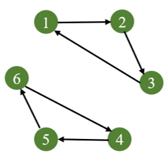
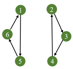
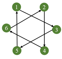
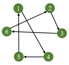
Example 1 Consider a WSN with $m=6$ sensors, whose dynamics obey (3)-(4) with $n=3$. The communication graph sequence $\big{\{}\mathcal{G}_{k}\big{\}}$ switches among $\mathcal{G}^{(1)}$, $\mathcal{G}^{(2)}$, $\mathcal{G}^{(3)}$ and $\mathcal{G}^{(4)}$ as shown in Figure 1. For all $u=1,2,3,4$, $a_{ij}^{(u)}=\frac{2}{5}$ if $(j,i)\in\mathcal{E}^{(u)}$; and 0, otherwise. The graph sequence $\left\{\mathcal{G}_{k}\right\}$ switches according to a Markovian chain $\{m_{k}\}$, with initial probability $p_{u,1}=\mathbb{P}\left\{\mathcal{G}_{1}=\mathcal{G}^{(u)}\right\}=$ $\frac{1}{4}$ and the following transition probability matrix:

$$\mathbf{P}=\left\{p_{uv}\right\}_{4\times 4}=\left[\begin{array}[]{cccc}{1}/{2}&{1}/{2}&0&0\\ 0&{1}/{2}&{1}/{2}&0\\ 0&0&{1}/{2}&{1}/{2}\\ {1}/{2}&0&0&{1}/{2}\end{array}\right]$$

where $p_{uv}=\mathbb{P}\left\{m_{k}=v\mid m_{k-1}=u\right\}$. Therefore, the stationary distribution $\pi_{u}=\frac{1}{4}$ for all $u=1,2,3,4$.

Refer to caption
(a) Graph $\mathcal{G}^{(1)}$
Refer to caption
(b) Graph $\mathcal{G}^{(2)}$
Refer to caption
(c) Graph $\mathcal{G}^{(3)}$
Refer to caption
(d) Graph $\mathcal{G}^{(4)}$
Figure 1: Switching communication topology

In the dynamic model (3), the unknown parameter $\theta=[1,1,-1]^{T}$ with prior information $\theta\in\Omega=[0,2]\times[-2,0]\times[0,2]$. The observation noise $d_{k,i}$ is independent and identically distributed Gaussian with zero mean and variance $8^{2}$. Let $\phi_{k,i}\in\mathbb{R}^{3}$ be generated by the following state space model

$$\begin{cases}x_{k,i}=A_{i}x_{k-1,i}+B_{i}\eta_{k,i},\\ \phi_{k,i}=C_{i}x_{k,i},\end{cases}i=1.,\ldots,6,$$

where $x_{k,i}\in\mathbb{R}^{3}$ with $x_{0,i}=[1.3,1.3,1.3]^{T}$, $\eta_{k,i}\in\mathbb{R}$ is independent and identically distributed with $\eta_{k,i}$ following uniform distribution on the interval $[-0.1,0.1]$ and

$\displaystyle A_{1}=\operatorname{diag}\{1,1/2,1/2\},A_{4}=\operatorname{diag}\{1,5/6,5/6\}$
$\displaystyle A_{2}=\operatorname{diag}\{1/2,1,1/2\},A_{5}=\operatorname{diag}\{5/6,1,5/6\},$
$\displaystyle A_{3}=\operatorname{diag}\{1/2,1/2,1\},A_{6}=\operatorname{diag}\{5/6,5/6,1\}$
$\displaystyle B_{1}=B_{4}=[1,0,0]^{T},B_{2}=B_{5}=[0,1,0]^{T},$
$\displaystyle B_{3}=B_{6}=[0,0,1]^{T},$
$\displaystyle C_{1}=\operatorname{diag}\{1,0,0\},C_{4}=\operatorname{diag}\{-1,0,0\},$
$\displaystyle C_{2}=\operatorname{diag}\{0,1,0\},C_{5}=\operatorname{diag}\{0,-1,0\},$
$\displaystyle C_{3}=\operatorname{diag}\{0,0,1\},C_{6}=\operatorname{diag}\{0,0,-1\},$

It can be verified that Assumption 2 is satisfied with $h=2$. Besides, the thresholds of quantized measurements are $C_{i}=1$ for all $i=1,\ldots,6$. In the quantized communication mechanism (4), the communication noise $\omega_{k,ij}$ is independent and identically distributed Gaussian with zero mean and variance $1$, and the threshold of quantized communications is $C_{ij}=0$ for all the channel $(j,i)\in\mathcal{E}_{\mathcal{C}}$.

Then, we apply the proposed EFTQDI algorithm with two types of step sizes to produce the estimates, where the linear encoding rule $\psi_{k}$ in (6) switches sequentially among $\{[1,0,0]^{T},[0,1,0]^{T},[0,0,1]^{T}\}$. The simulation is repeated $100$ times using the same initial values $\hat{\theta}_{0,ij}=[1/2,1/2,1/2]$ and ${\theta}_{0,i}=[1/2,1/2,1/2]$ to calculate the empirical variance of estimation errors, representing the mean square errors.

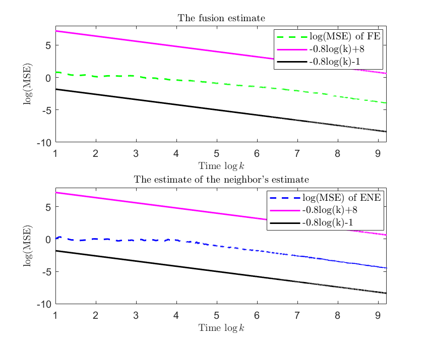
In the first case, the step size for the proposed EFTQDI algorithm is set as $b_{k}=\frac{1}{k}$ with the step coefficients $\beta=39$ and $\gamma=74$. The mean square errors (MSEs) of both the fusion estimate (FE) and the estimate of the neighboring estimate (ENE) are shown in Figure 2. These results indicate that the fusion estimate and ENE converge to the true parameter and fusion estimate, respectively. Additionally, Figure 3 shows a linear relationship between the logarithm of the MSEs and the logarithm of the index $k$, which indicates the mean square convergence rates of the estimation errors are $O(\frac{1}{k})$.

Refer to caption
Figure 2: Convergence of the two estimates with $b_{k}=\frac{1}{k}$.
Refer to caption
Figure 3: Convergence rate of the two estimates with $b_{k}=\frac{1}{k}$.

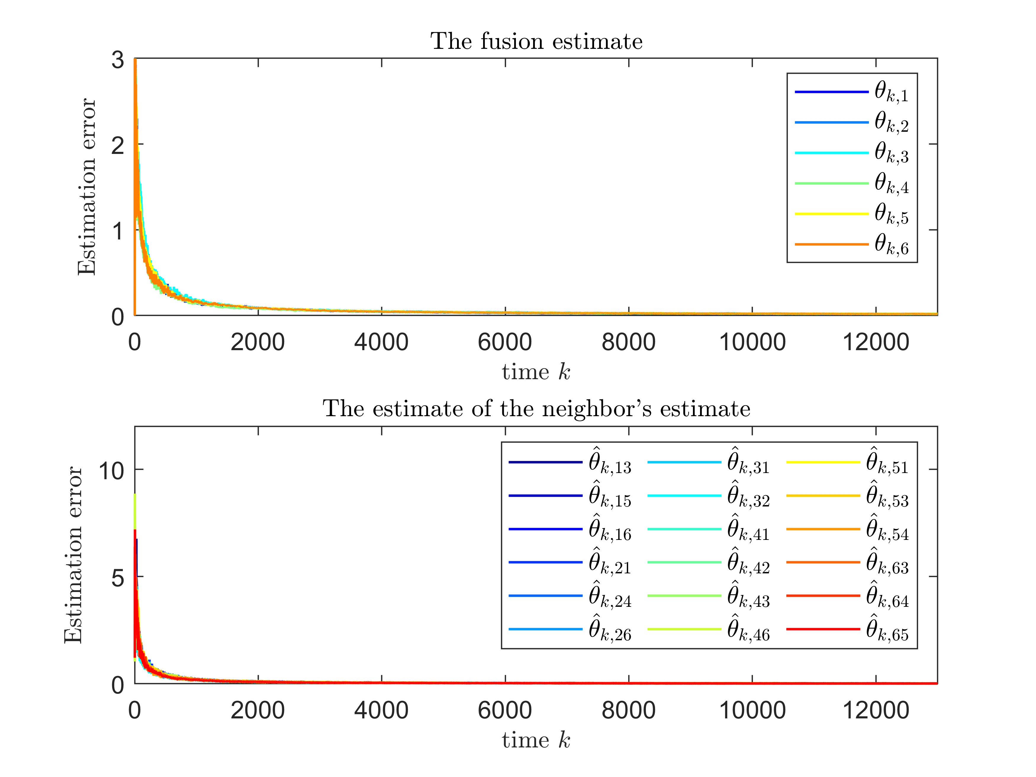
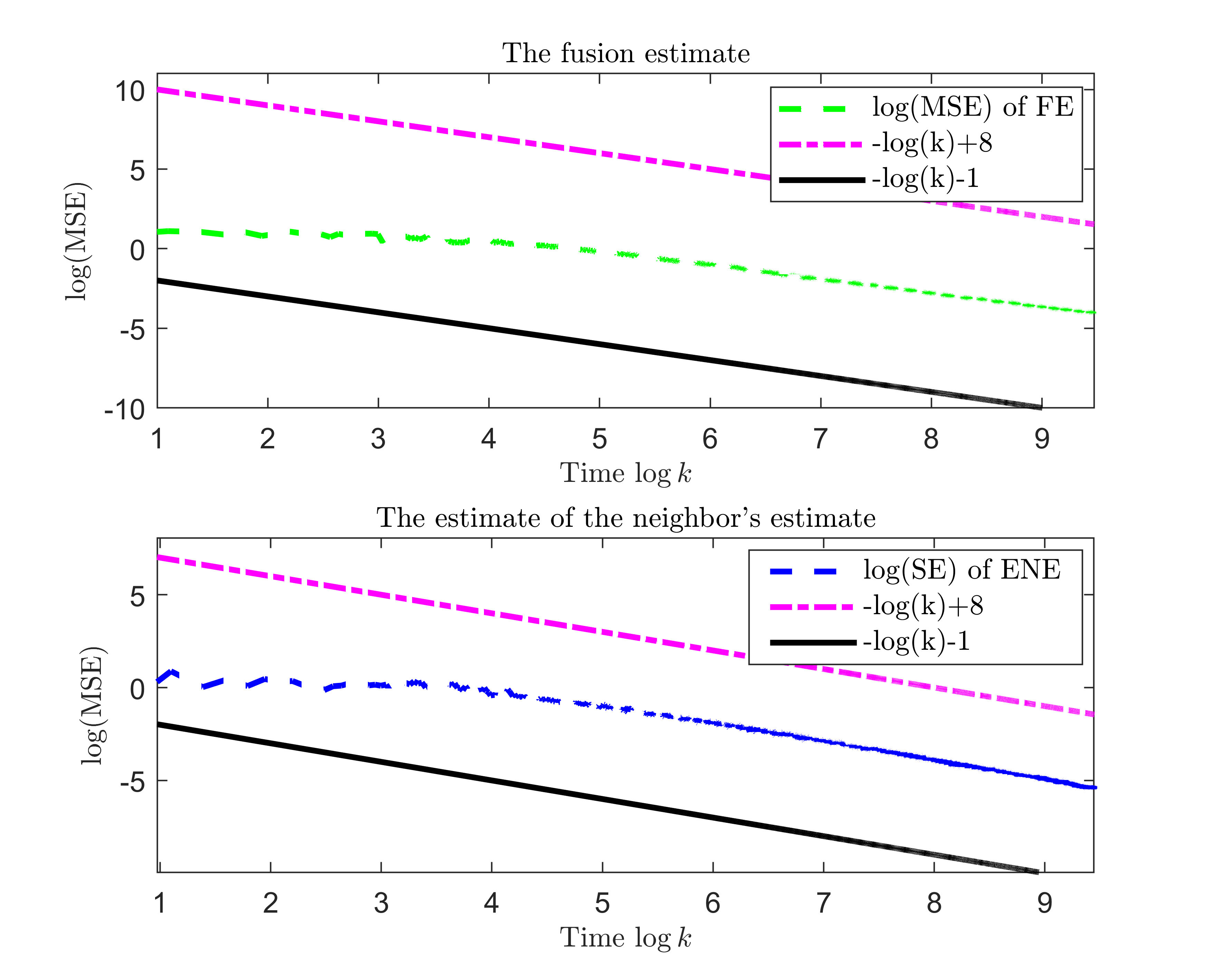
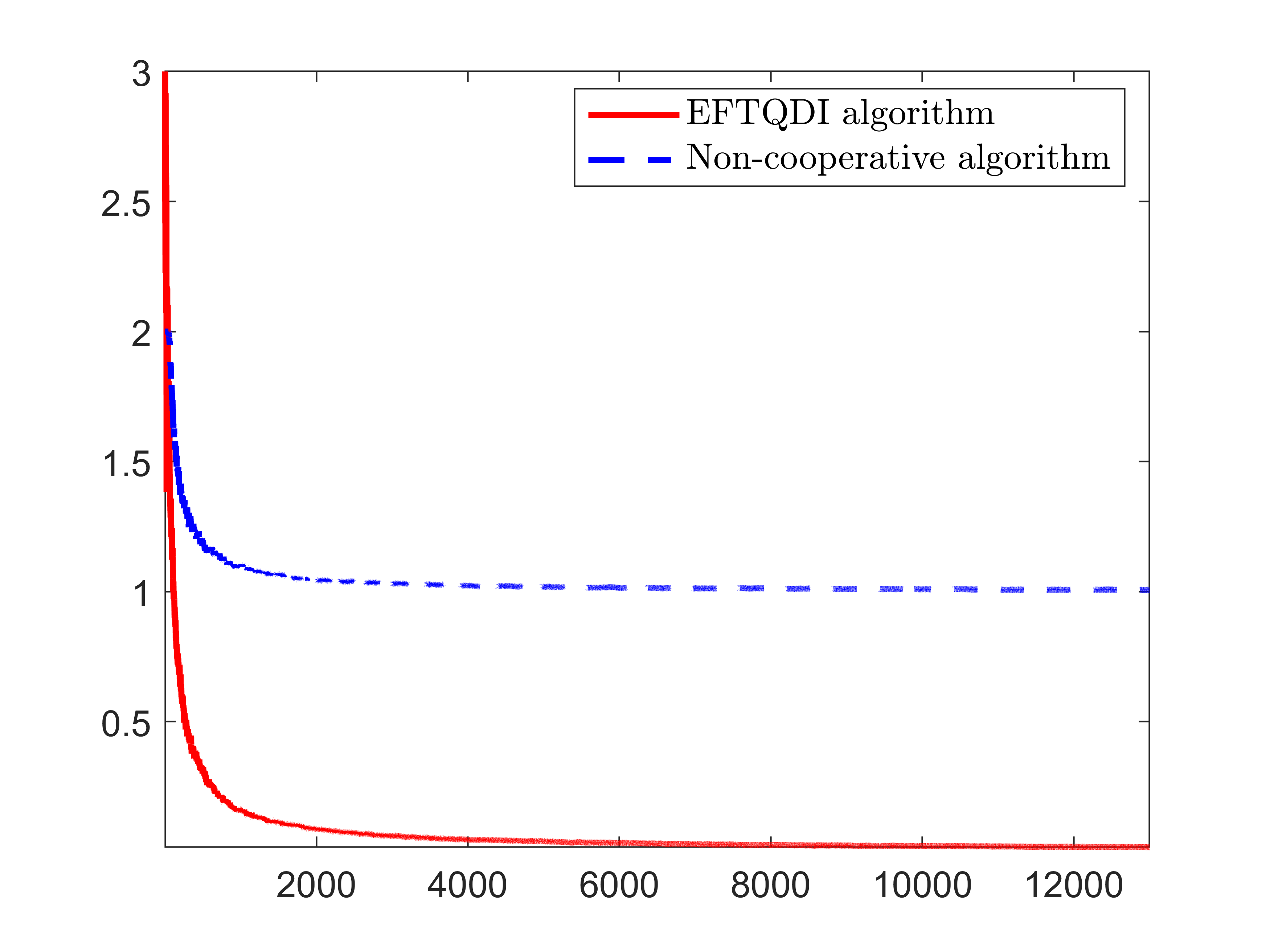
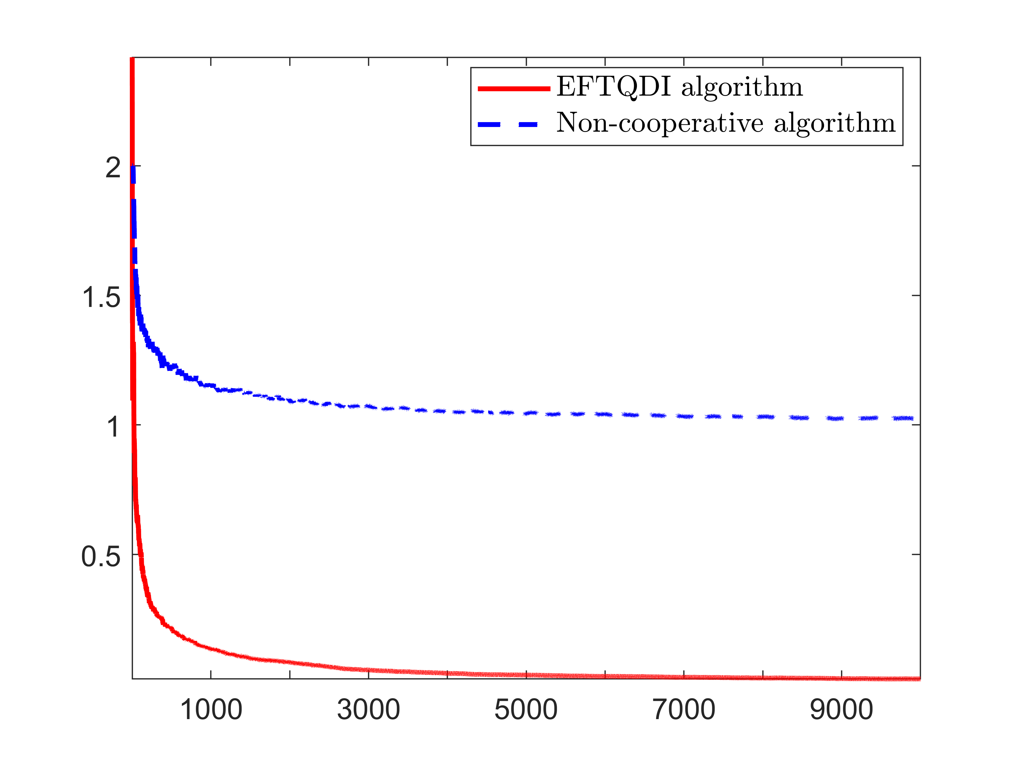
Figure 4 shows the MSEs trajectories of the proposed EFTQDI algorithm compared to its non-cooperative counterpart (i.e., ${\theta}_{k,i}=\Pi_{\Omega}\{{\theta}_{k-1,i}+\beta b_{k}\phi_{k,i}(\hat{F}_{k,i}-s_{k,i})\}$). The results indicate that, unlike the non-cooperative algorithm, which does not converge to zero, the EFTQDI algorithm’s estimate converges to the true parameter. This highlights the joint effect of sensors under quantized communication, as one-bit information exchange among sensors enables the estimation task that individual sensors cannot achieve alone.

Refer to caption
Figure 4: The comparison between the EFTQDI algorithm and non-cooperative algorithm under $b_{k}=\frac{1}{k}$.

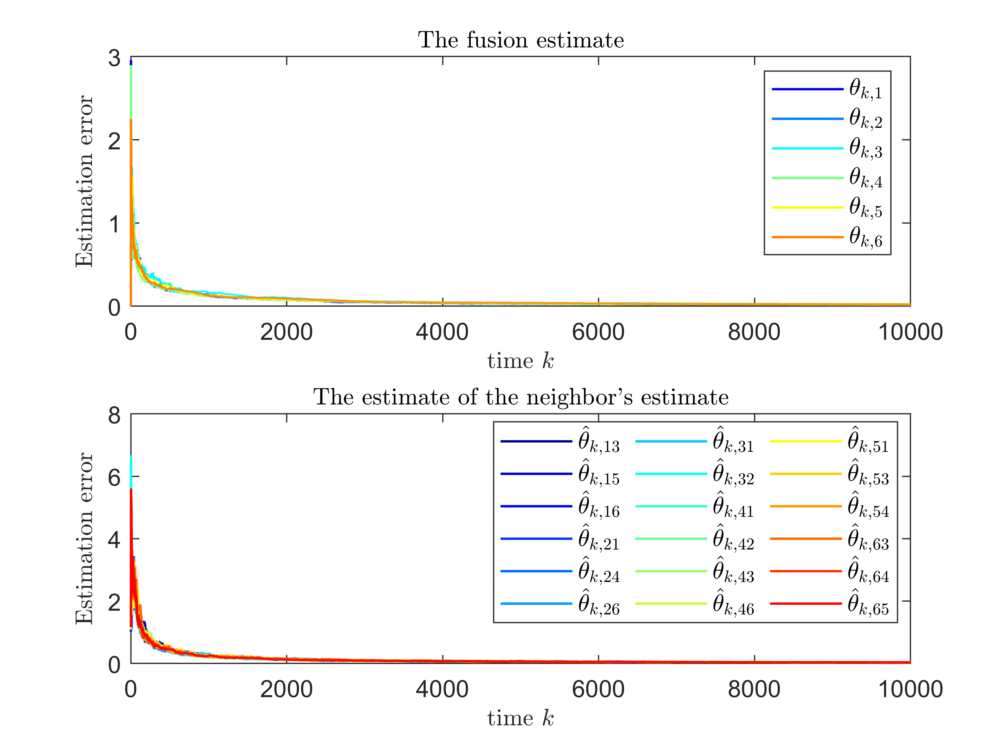
In the second case, the step size in the EFTQDI algorithm is set as $b_{k}=\frac{1}{k^{4/5}}$ with step coefficients $\beta=16$ and $\gamma=65$. Figure 5 shows that both the fusion estimate and the estimate of the neighboring estimate converge, respectively. Besides, Figure 6 shows that the logarithms of MSEs of the two estimates scale linearly with $\frac{4}{5}\log k$, indicating a mean square convergence rate of $O(\frac{1}{k^{4/5}})$. Figure 7 shows the MSE trajectories of the EFTQDI algorithm and its corresponding non-cooperative algorithm, which demonstrates again the joint effect of the sensors under quantized communication.

Refer to caption
Figure 5: Convergence of the two estimates with $b_{k}=\frac{1}{k^{4/5}}$.

7 Conclusion

This paper addresses distributed parameter estimation in stochastic dynamic systems with quantized measurements, focusing on quantized communication and Markov-switching directed topologies. A compression encoding method satisfying persistent excitation is introduced, ensuring original signal recovery from quantized transmitted data. Based on this, an EFTQDI algorithm is proposed, leveraging a stochastic approximation idea. This approach first estimates the neighboring estimates through quantized communication, followed by a consensus-based fusion strategy to integrate these estimates. By constructing and analyzing two coupled Lyapunov functions for estimation errors, we establish the mean-square convergence of these two estimates under a cooperative excitation condition and the assumption that the union topology includes a spanning tree. Furthermore, we demonstrate that the mean-square convergence rate aligns with the step size order given appropriate coefficient conditions.

Future work could explore the combination of event-driven mechanisms and quantized protocol, which both can reduce communication load. Developing effective event-driven quantized transmission protocols to ensure distributed estimation with minimal data transfer remains a compelling challenge.

Refer to caption
Figure 6: Convergence rate of the two estimates with $b_{k}=\frac{1}{k^{4/5}}$.
Refer to caption
Figure 7: The comparison between the EFTQDI algorithm and non-cooperative algorithm under $b_{k}=\frac{1}{k^{4/5}}$.

References

  • Akyildiz et al. (2002) Akyildiz, I. F., Su, W., Sankarasubramaniam, Y., Cayirci, E., (2002). Wireless sensor networks: a survey. Computer Networks, 38, 393–422.
  • Bianchi et al. (2013) Bianchi, P., Fort, G., Hachem, W., (2013). Performance of a distributed stochastic approximation algorithm. IEEE Transactions on Information Theory, 59, 7405–7418.
  • Calamai and Moré (1987) Calamai, P. H., Moré, J.J., (1987). Projected gradient methods for linearly constrained problems. Mathematical Programming, 39, 93–116.
  • Dimakis et al. (2010) Dimakis, A., Kar, S., Moura, J., Rabbat, M., Scaglione, A., (2010). Gossip algorithms for distributed signal processing. Proceedings of the IEEE, 98, 1847–1864.
  • Ding et al. (2017) Ding, D., Wang, Z., Ho, D., Wei, G., (2017). Distributed recursive filtering for stochastic systems under uniform quantizations and deception attacks through sensor networks. Automatica, 78, 231–240.
  • Fu et al. (2022) Fu, K., Chen, H. F., Zhao, W., (2022). Distributed system identification for linear stochastic systems with binary sensors. Automatica, 141, 110298.
  • Gan and Liu (2024) Gan, D., Liu, Z., (2024). Convergence of the distributed SG algorithm under cooperative excitation condition. IEEE Transactions on Neural Networks and Learning Systems, 35, 7087–7101.
  • Ge et al. (2020) Ge, X., Han, Q. L., Zhang, X., Ding, L., Yang, F., (2020). Distributed event-triggered estimation over sensor networks: A survey. IEEE Transactions on Cybernetics, 50, 1306–1320.
  • Guo and Zhao (2013) Guo, J., Zhao, Y. L., (2013). Recursive projection algorithm on FIR system identification with binary-valued observations. Automatica, 49, 3396–3401.
  • Han et al. (2023a) Han, F., Wang, Z., Dong, H., Yi, X., Alsaadi, F., (2023)a. Distributed $h_{\infty}$-consensus estimation for random parameter systems over binary sensor networks: A local performance analysis method. IEEE Transactions on Network Science and Engineering, 10, 2334–2346.
  • Han et al. (2023b) Han, F., Wang, Z., Dong, H., Yi, X., Alsaadi, F., (2023)b. Recursive distributed filtering for time-varying systems over sensor network via rayleigh fading channels: Tackling binary measurements. IEEE Transactions on Signal and Information Processing over Networks, 9, 110–122.
  • Huang et al. (2010) Huang, M., Dey, S., Nair, G., Manton, J., (2010). Stochastic consensus over noisy networks with markovian and arbitrary switches. Automatica, 46, 1571–1583.
  • Kar et al. (2012) Kar, S., Moura, J., Ramanan, K., (2012). Distributed parameter estimation in sensor networks: Nonlinear observation models and imperfect communication. IEEE Transactions on Information Theory, 58, 3575–3605.
  • Lei and Chen (2020) Lei, J., Chen, H. F., (2020). Distributed stochastic approximation algorithm with expanding truncations. IEEE Transactions on Automatic Control, 65, 664–679.
  • Li et al. (2023) Li, J., Wang, Z., Lu, R., Xu, Y., (2023). Distributed filtering under constrained bit rate over wireless sensor networks: Dealing with bit rate allocation protocol. IEEE Transactions on Automatic Control, 68, 1642–1654.
  • Li and Zhang (2010) Li, T., Zhang, J. F., (2010). Consensus conditions of multi-agent systems with time-varying topologies and stochastic communication noises. IEEE Transactions on Automatic Control, 55, 2043–2057.
  • Mateos and Giannakis (2012) Mateos, G., Giannakis, G., 2012. Distributed recursive least-squares: Stability and performance analysis. IEEE Transactions on Signal Processing, 60, 3740–3754.
  • Polyak (1987) Polyak, B., (1987). Introduction to Optimization. New York: Optimization Soft-ware Inc.,
  • Pottie and Kaiser (2000) Pottie, G., Kaiser, W., (2000). Wireless integrated network sensors. Communications of the ACM, 43, 51–58.
  • Rawat et al. (2014) Rawat, P., Singh, K., Chaouchi, H., Bonnin, J., (2014). Wireless sensor networks: a survey on recent developments and potential synergies. The Journal of Supercomputing, 68, 1–48.
  • Ren and Beard (2005) Ren, W., Beard, R., (2005). Consensus seeking in multiagent systems under dynamically changing interaction topologies. IEEE Transactions on Automatic Control, 50, 655–661.
  • Seneta (2006) Seneta, E., (2006). Non-negative Matrices and Markov Chains. Springer: NY, USA.
  • Sinha and Griscik (1971) Sinha, N., Griscik, M., (1971). A stochastic approximation method. IEEE Transactions on Systems, Man, and Cybernetics, SMC-1, 338–344.
  • Swenson et al. (2020) Swenson, B., Sridhar, A., Poor, H., (2020). On distributed stochastic gradient algorithms for global optimization, in: ICASSP 2020 - 2020 IEEE International Conference on Acoustics, Speech and Signal Processing, pp. 8594–8598.
  • Taj and Cavallaro (2011) Taj, M., Cavallaro, A., (2011). Distributed and decentralized multicamera tracking. IEEE Signal Processing Magazine, 28, 46–58.
  • Takahashi et al. (2010) Takahashi, N., Yamada, I., Sayed, A., (2010). Diffusion least-mean squares with adaptive combiners: Formulation and performance analysis. IEEE Transactions on Signal Processing, 58, 4795–4810.
  • Wang et al. (2024) Wang, J., Ke, J., Zhang, J. F., (2024). Differentially private bipartite consensus over signed networks with time-varying noises. IEEE Transactions on Automatic Control, 69, 5788–5803.
  • Wang et al. (2018) Wang, T., Tan, J., Zhao, Y. L., (2018). Asymptotically efficient non-truncated identification for FIR systems with binary-valued outputs. Science China Information Sciences, 61, 129208.
  • Wang et al. (2003) Wang, L. Y., Zhang, J. F., Yin, G., (2003). System identification using binary sensors. IEEE Transactions on Automatic Control, 48, 1892–1907.
  • Wang and Zhang (2019) Wang, Y., Zhang, J. F., (2019). Distributed parameter identification of quantized ARMAX systems, in: Proceedings of the 38th Chinese Control Conference, pp. 1701–1706.
  • Wang et al. (2021) Wang, Y., Zhao, Y. L., Zhang, J. F., (2021). Distributed recursive projection identification with binary-valued observations. Journal of Systems Science and Complexity, 34, 2048–2068.
  • Wang et al. (2022) Wang, Y., Zhao, Y. L., Zhang, J. F., Guo, J., (2022). A unified identification algorithm of FIR systems based on binary observations with time-varying thresholds. Automatica, 135, 109990.
  • Xie and Guo (2018) Xie, S., Guo, L., (2018). Analysis of normalized least mean squares-based consensus adaptive filters under a general information condition. SIAM Journal on Control and Optimization, 56, 3404–3431.
  • Xie et al. (2021) Xie, S., Zhang, Y., Guo, L., (2021). Convergence of a distributed least squares. IEEE Transactions on Automatic Control, 66, 4952–4959.
  • You (2015) You, K., (2015). Recursive algorithms for parameter estimation with adaptive quantizer. Automatica, 52, 192–201.
  • Zhang et al. (2021) Zhang, H., Wang, T., Zhao, Y. L., (2021). Asymptotically efficient recursive identification of FIR systems with binary-valued observations. IEEE Transactions on Systems, Man, and Cybernetics: Systems, 51, 2687–2700.
  • Zhang et al. (2022) Zhang, L., Zhao, Y. L., Guo, L., (2022). Identification and adaptation with binary-valued observations under non-persistent excitation condition. Automatica, 138, 110158.
  • Zhang and Zhang (2012) Zhang, Q., Zhang, J. F., (2012). Distributed parameter estimation over unreliable networks with markovian switching topologies. IEEE Transactions on Automatic Control, 57, 2545–2560.
  • Zhao et al. (2023) Zhao, Y. L., Zhang, H., Kang, G., (2023). System identification under saturated precise or set-valued measurements. Science China Information Sciences, 66, 112204.
  • Zhu et al. (2018) Zhu, S., Chen, C., Xu, J., Guan, X., Xie, L., Johansson, K. H., (2018). Mitigating quantization effects on distributed sensor fusion: A least squares approach. IEEE Transactions on Signal Processing, 66, 3459–3474.
  • Zhu et al. (2017) Zhu, S., Liu, S., Soh, Y., Xie, L., (2017). Performance analysis of averaging based distributed estimation algorithm with additive quantization model. Automatica, 80, 95–101.
  • Zhu et al. (2015) Zhu, S., Soh, Y., Xie, L., (2015). Distributed parameter estimation with quantized communication via running average. IEEE Transactions on Signal Processing, 63, 4634–4646.