Soliton solutions associated with the third-order ordinary linear differential operator

Abstract

Explicit solutions to the related integrable nonlinear evolution equations are constructed by solving the inverse scattering problem in the reflectionless case for the third-order differential equation $d^{3}\psi/dx^{3}+Q\,d\psi/dx+P\psi=k^{3}\psi,$ where $P$ and $Q$ are the potentials in the Schwartz class and $k^{3}$ is the spectral parameter. The input data set used to solve the relevant inverse problem consists of the bound-state poles of a transmission coefficient and the corresponding bound-state dependency constants. Using the time-evolved dependency constants, explicit solutions to the related integrable evolution equations are obtained. In the special cases of the Sawada–Kotera equation, the Kaup–Kupershmidt equation, and the bad Boussinesq equation, the method presented here explains the physical origin of the constants appearing in the relevant $\mathbf{N}$-soliton solutions algebraically constructed, but without any physical insight, by the bilinear method of Hirota.

AMS Subject Classification (2020):

Keywords: inverse scattering for the third-order equation, bound-state dependency constants, soliton solutions, Sawada–Kotera equation, Kaup–Kupershmidt equation, bad Boussinesq equation

1 Introduction

Consider the third-order linear ordinary differential equation on the line given by

$$\psi^{\prime\prime\prime}+Q(x,t)\,\psi^{\prime}+P(x,t)\,\psi=k^{3}\,\psi,\qquad x\in\mathbb{R},$$ (1.1)

where $x$ is the independent variable representing the spacial coordinate and taking values on the real line $\mathbb{R},$ the prime denotes the $x$-derivative, $t$ is a parameter representing the time coordinate, $k^{3}$ is the spectral parameter, and the coefficients $Q$ and $P$ are some complex-valued functions of $x$ and $t$ vanishing rapidly as $x\to\pm\infty$ for each fixed $t\in\mathbb{R}.$ For simplicity, we assume that $Q$ and $P$ belong to the Schwartz class $S(\mathbb{R})$ in the $x$-variable, which is the class of infinitely differentiable functions $\theta(x)$ in such a way that $x^{j}d^{l}\theta(x)/dx^{l}$ vanishes as $x\to\pm\infty$ for any pair of nonnegative integers $j$ and $l.$ We refer to $Q$ and $P$ as the potentials. Our results hold under weaker assumptions on $Q$ and $P,$ but for simplicity we assume that the potentials $Q$ and $P$ belong to the Schwartz class in $x.$

We can write (1.1) as $L\psi=\lambda\psi$ by letting $\lambda:=k^{3}$ and defining the linear differential operator $L$ as

$$L:=D^{3}+QD+P,$$ (1.2)

where we use $D$ to represent the differential operator $d/dx.$ Let us also introduce the linear differential operator $A$ given by

$$A:=9\,D^{5}+15\,QD^{3}+\big{(}15\,P+15\,Q_{x}\big{)}D^{2}+\big{(}15\,P_{x}+10\,Q_{xx}+5\,Q^{2}\big{)}D+\big{(}10\,P_{xx}+10\,Q\,P\big{)},$$ (1.3)

where we use the subscripts $x$ and $t$ to denote the appropriate partial derivatives. Using (1.2) and (1.3) we would like to have [23]

$$L_{t}+LA-AL=0,$$ (1.4)

where $L_{t}$ is the differential operator given by

$$L_{t}=Q_{t}D+P_{t}.$$ (1.5)

It can be verified directly that the Lax compatibility equation (1.4) is satisfied by (1.2), (1.3), and (1.5) provided that the potentials $Q$ and $P$ satisfy the coupled system of two fifth-order nonlinear partial differential equations given by

$$\begin{cases}Q_{t}+Q_{xxxxx}+5\,Q_{x}\,Q_{xx}+5\,Q\,Q_{xxx}+5\,Q^{2}\,Q_{x}+15\,Q_{xx}\,P+15\,Q_{x}\,P_{x}-30\,P\,P_{x}=0,\\ \vskip 6.0pt plus 2.0pt minus 2.0pt\cr\begin{aligned} P_{t}+P_{xxxxx}+5\,Q\,P_{xxx}+15\,Q_{x}\,P_{xx}+20\,Q_{xx}\,P_{x}+5\,Q^{2}\,P_{x}+&10\,Q_{xxx}\,P-15\,P\,P_{xx}\\ &+10\,Q\,Q_{x}P-15\,P_{x}^{2}=0,\end{aligned}\end{cases}$$ (1.6)

where we have $x\in\mathbb{R}$ and the $t$-domain can be chosen either as $\mathbb{R}$ or $t>0.$ Thus, the system given in (1.6) is integrable in the sense of the inverse scattering transform method [16], and its initial-value problem can be solved with the help of the direct and inverse scattering theory for (1.1) with the appropriate time evolution of the scattering data governed by the linear operator $A$ in (1.3).

For simplicity, we choose our notation by suppressing the appearance of $t$ in the arguments of the potentials and all other quantities associated with (1.1) and (1.6). In particular, we use $Q(x)$ instead of $Q(x,t)$ and write $P(x)$ instead of $P(x,t).$

The uncoupled version of (1.6) is obtained when the sum of the last three terms on the left-hand side of the first equality of (1.6) vanishes, i.e. when we have

$$15\,Q_{xx}P+15\,Q_{x}\,P_{x}-30\,P\,P_{x}=0.$$ (1.7)

Integrating (1.7) and using the fact that the potentials $Q$ and $P$ vanish as $x\to\pm\infty,$ we get

$$Q_{x}P-P^{2}=0.$$ (1.8)

From (1.8), we observe that (1.6) has exactly two special cases given by

$$P(x)\equiv 0,\quad P(x)\equiv Q_{x}(x).$$ (1.9)

In the first special case $P(x)\equiv 0,$ the integrable system (1.6) reduces to the single integrable evolution equation

$$Q_{t}+Q_{xxxxx}+5\,Q_{x}\,Q_{xx}+5\,Q\,Q_{xxx}+5\,Q^{2}\,Q_{x}=0,\qquad x,\,t\in\mathbb{R},$$ (1.10)

which is known as the Sawada–Kotera equation [19, 20, 29]. In applications, the quantity $Q$ in the Sawada–Kotera equation is usually assumed to be real valued. In the second special case $P(x)\equiv Q_{x}(x),$ the integrable system (1.6) again reduces to the single integrable evolution equation given in (1.10). In this second special case, the integrable evolution equation (1.10) is known as the Kaup–Kupershmidt equation [20, 22]. In applications, the quantity $Q$ in the Kaup–Kupershmidt equation is also usually assumed to be real valued.

In this paper we are interested in exploring explicit solutions to the integrable system (1.6) and its two special cases given in (1.10). In the literature some specific explicit solutions to (1.10) are obtained usually by using Hirota’s bilinear method [19] or by using the dressing method of Zakharov and Shabat [27], where both these methods avoid the analysis of the direct and inverse scattering problems associated with (1.1). Such explicit solutions, if they do not contain any singularities, correspond to soliton solutions. Our goal is to obtain those explicit solutions, without using an ansatz but only by relying on the analysis of the direct and inverse scattering problems for (1.1). In general, soliton solutions for integrable systems correspond to reflectionless scattering data sets, which consist of transmission coefficients and time-evolved bound-state information. The bound-state information can be provided by specifying the poles of the transmission coefficients and the bound-state normalization constants or bound-state dependency constants. Hence, in this paper we describe soliton solutions for (1.6) and its two special cases given in (1.10), without using any ansatzes but by using the transmission coefficients and the time-evolved bound-state data for (1.1), where the bound-state data set consists of the $k$-values specifying the bound-state poles of the transmission coefficients and the bound-state dependency constants at those $k$-values. Since the differential operator $L$ appearing in (1.2) is not selfadjoint, in case the bound states have any multiplicities it is understood that for each bound state we have as many dependency constants as the multiplicity of that bound state.

The most relevant references related to the research presented in this paper are the 1980 paper [20] by Kaup, the 1982 paper [11] by Deift, Tomei, and Trubowitz, the 1989 paper [19] by Hirota, the 2001 paper [27] by Parker, the 2002 paper [21] by Kaup, and the Ph.D. thesis [30] of the third author of the present paper. Kaup initiated [20] the analysis of the direct and inverse scattering for (1.1) with the goal of studying solutions to the integrable nonlinear evolution equation (1.10). However, he was unable to formulate a proper scattering matrix and a proper Riemann–Hilbert problem associated with (1.1). We refer to a Riemann–Hilbert problem as properly formulated if the plus and minus regions in the complex plane are separated by an infinite straight line passing through the origin. Such a formulation allows the use of a Fourier transformation along that line. For example, in the analysis of the inverse scattering problem for the Schrödinger equation on the full line, we have a proper formulation of the Riemann–Hilbert problem with the real axis separating the complex plane into two regions. Such a formulation enables the use of a Fourier transformation, which yields the Marchenko integral equation [8, 10, 12, 15, 24, 25] playing a key role in the solution to the corresponding inverse scattering problem. The lack of a proper formulation of a Riemann–Hilbert problem for (1.1) prevented Kaup from establishing [21] a linear integral equation, which would be the analog of the Marchenko integral equation associated with the inverse scattering problem for the full-line Schrödinger equation. Deift, Tomei, and Trubowitz studied [11] the direct and inverse scattering problems for a special case of (1.1), namely for the third-order equation (6.4) listed in Section 6. Even though the linear operator $L$ given in (1.2) associated with (1.1) is in general not selfadjoint, the linear operator $L$ given in (6.2) of Section 6 associated with (6.4) is selfadjoint. Deift, Tomei, and Trubowitz introduced [11] a proper Riemann–Hilbert problem on the complex $k$-plane, enabling them to solve the corresponding inverse scattering problem for (6.4). However, in order to formulate their Riemann–Hilbert problem, they used the severe assumption that the two transmission coefficients associated with (6.4) are identically equal to $1$ for all $k$-values. They also used the assumption that the two secondary reflection coefficients are identically zero. That latter assumption is not as severe as the former assumption, and in fact it helps to discard solutions to (6.5) that blow up at finite time. The former assumption prevented Deift, Tomei, and Trubowitz from obtaining explicit solutions to (6.5). This is because such solutions are usually obtained in the reflectionless case by using the bound-state poles of the transmission coefficients. Hirota used his bilinear method to obtain the $\mathbf{N}$-soliton solution [18] to the bad Boussinesq equation and the $\mathbf{N}$-soliton solution [19] to the Sawada–Kotera equation. Those ad hoc solutions were introduced algebraically by Hirota without any connection to the direct and inverse scattering theory associated with the corresponding linear third-order equations. Parker [27] tried to explain the derivation of Hirota’s ad hoc $\mathbf{N}$-soliton solutions to the Sawada–Kotera equation by using a modification of the dressing method [31] of Zakharov and Shabat. In his 2002 review paper [21] Kaup summarized the efforts on the inverse scattering transform associated with the third-order equation (1.1) in the two special cases given in (1.9), but without mentioning the relevant paper [11] by Deift, Tomei, and Trubowitz. Inspired by [11], Toledo formulated [30] a proper Riemann–Hilbert problem associated with the inverse scattering problem for (1.1) by only using the assumption that the two secondary reflection coefficients are identically zero, but without using the assumption that the two transmission coefficients are identically equal to $1$ for all $k$-values.

Our paper uses the method of [30] in the reflectionless case, and it is organized as follows. In Section 2 we present a brief summary of the direct scattering problem for (1.1) by introducing the basic solutions to (1.1) and the scattering coefficients for (1.1) and by providing the relevant properties of those solutions and scattering coefficients. We also present the time evolutions of the basic solutions and the scattering coefficients when the potentials $Q$ and $P$ in (1.1) depend on the temporal parameter $t.$ In Section 3 we provide a brief description of the bound states associated with (1.1) and the corresponding bound-state dependency constants. In Section 4 we consider (1.1) in the reflectionless case, and we formulate the Riemann–Hilbert problem in the complex $k$-plane by introducing the relevant plus and minus regions and the plus and minus functions in those regions. We also describe how the potentials $Q$ and $P$ are recovered from the solution to the aforementioned Riemann–Hilbert problem. In Section 5 we show how explicit solution to (1.1) are constructed by solving the relevant Riemann–Hilbert problem using the input data set consisting of the bound-state poles of a transmission coefficient and the corresponding bound-state dependency constants. With the input data set containing the time-evolved dependency constants, the constructed potentials $Q$ and $P$ yield explicit solutions to (1.6). By using the appropriate restrictions on the locations of the bound-state $k$-values and the appropriate restrictions on the dependency constants, we obtain real-valued solutions to (1.10) in the two special cases of the Sawada–Kotera equation and the Kaup–Kupershmidt equation. In fact, we show that Hirota’s $\mathbf{N}$-soliton solution to the Sawada–Kotera equation can be obtained from a particular $2\mathbf{N}$-soliton solution to (1.6) by using some appropriate restrictions on our input data set. Hence, our method using the input data set consisting of the bound-state poles of a transmission coefficient and the corresponding time-evolved bound-state dependency constants explains the physical origin of the $\mathbf{N}$-soliton solution to the Sawada–Kotera equation algebraically constructed [19] by the bilinear method of Hirota. Similarly, we show that the $\mathbf{N}$-soliton solution to the Kaup–Kupershmidt equation can be obtained from our same particular $2\mathbf{N}$-soliton solution to (1.6). Since our method is based on the solution to the inverse scattering problem for (1.1) in the reflectionless case, it is applicable on all integrable evolution equations associated with (1.1). This is further illustrated in Section 6, where we show how our method yields explicit solutions to the bad Boussinesq equation, again explaining the physical origin of the $\mathbf{N}$-soliton solution obtained by Hirota’s method [18].

2 The direct scattering problem

In this section we present a summary of the direct scattering theory for the third-order equation (1.1). We recall that we suppress the appearance of the parameter $t$ in the arguments of the quantities related to (1.1). We choose the notation used in the recent Ph.D. thesis [30] of the third author.

It is convenient to use the four directed half lines $\mathcal{L}_{1},$ $\mathcal{L}_{2},$ $\mathcal{L}_{3},$ $\mathcal{L}_{4}$ to divide the complex $k$-plane $\mathbb{C}$ into the four sectors $\Omega_{1},$ $\Omega_{2},$ $\Omega_{3},$ $\Omega_{4}$ as shown in Figure 2.1.

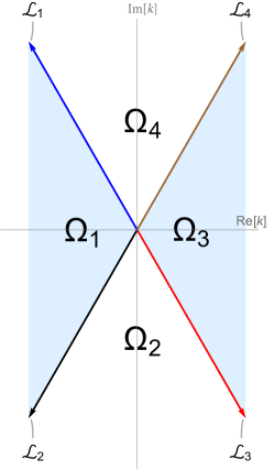
Figure 2.1: The directed half lines $\mathcal{L}_{1},$ $\mathcal{L}_{2},$ $\mathcal{L}_{3},$ $\mathcal{L}_{4}$ and the open sectors $\Omega_{1},$ $\Omega_{2},$ $\Omega_{3},$ $\Omega_{4}$ in the complex $k$-plane.

We use $z$ to denote the special complex number $e^{2\pi i/3},$ which is equivalently defined as

$$z:=-\displaystyle\frac{1}{2}+i\,\displaystyle\frac{\sqrt{3}}{2}.$$ (2.1)

The directed half lines $\mathcal{L}_{1},$ $\mathcal{L}_{2},$ $\mathcal{L}_{3},$ $\mathcal{L}_{4}$ are defined by the respective parametrizations given by

$$\mathcal{L}_{1}:=\{k\in\mathbb{C}:k=zs\text{\rm{ for }}s\in[0,+\infty)\},$$ (2.2)

$$\mathcal{L}_{2}:=\{k\in\mathbb{C}:k=z^{2}s\text{\rm{ for }}s\in[0,+\infty)\},$$ (2.3)

$$\mathcal{L}_{3}:=\{k\in\mathbb{C}:k=-zs\text{\rm{ for }}s\in[0,+\infty)\},$$ (2.4)

$$\mathcal{L}_{4}:=\{k\in\mathbb{C}:k=-z^{2}s\text{\rm{ for }}s\in[0,+\infty)\}.$$ (2.5)

As seen from Figure 2.1, the four open sectors $\Omega_{1},$ $\Omega_{2},$ $\Omega_{3},$ $\Omega_{4}$ in $\mathbb{C}$ are respectively defined by using the parametrizations given by

$$\Omega_{1}:=\left\{k\in\mathbb{C}:\displaystyle\frac{2\pi}{3}<\arg[k]<\displaystyle\frac{4\pi}{3}\right\},$$ (2.6)

$$\Omega_{2}:=\left\{k\in\mathbb{C}:-\displaystyle\frac{2\pi}{3}<\arg[k]<-\displaystyle\frac{\pi}{3}\right\},$$ (2.7)

$$\Omega_{3}:=\left\{k\in\mathbb{C}:-\displaystyle\frac{\pi}{3}<\arg[k]<\displaystyle\frac{\pi}{3}\right\},$$ (2.8)

$$\Omega_{4}:=\left\{k\in\mathbb{C}:\displaystyle\frac{\pi}{3}<\arg[k]<\displaystyle\frac{2\pi}{3}\right\},$$ (2.9)

where $\arg[k]$ represents the argument function taking values in the interval $(-2\pi/3,4\pi/3).$ We use $\overline{\Omega_{1}},$ $\overline{\Omega_{2}},$ $\overline{\Omega_{3}},$ $\overline{\Omega_{4}}$ to denote the closures of $\Omega_{1},$ $\Omega_{2},$ $\Omega_{3},$ $\Omega_{4},$ respectively. Thus, the closed sector $\overline{\Omega_{1}}$ is obtained from $\Omega_{1}$ by including its respective upper and lower boundaries $\mathcal{L}_{1}$ and $\mathcal{L}_{2},$ the closed sector $\overline{\Omega_{2}}$ is obtained from $\Omega_{2}$ by including its respective left and right boundaries $\mathcal{L}_{2}$ and $\mathcal{L}_{3},$ the closed sector $\overline{\Omega_{3}}$ is obtained from $\Omega_{3}$ by including its respective lower and upper boundaries $\mathcal{L}_{3}$ and $\mathcal{L}_{4},$ and the closed sector $\overline{\Omega_{4}}$ is obtained from $\Omega_{4}$ by including its respective left and right boundaries $\mathcal{L}_{1}$ and $\mathcal{L}_{4}.$

The left Jost solution $f(k,x)$ to (1.1) is defined as the solution satisfying the spacial asymptotics

$$\begin{cases}f(k,x)=e^{kx}\left[1+o(1)\right],\qquad x\to+\infty,\\ \vskip 6.0pt plus 2.0pt minus 2.0pt\cr f^{\prime}(k,x)=k\,e^{kx}\left[1+o(1)\right],\qquad x\to+\infty,\\ \vskip 6.0pt plus 2.0pt minus 2.0pt\cr f^{\prime\prime}(k,x)=k^{2}\,e^{kx}\left[1+o(1)\right],\qquad x\to+\infty.\end{cases}$$ (2.10)

The right Jost solution $g(k,x)$ to (1.1) is defined as the solution satisfying the spacial asymptotics

$$\begin{cases}g(k,x)=e^{kx}\left[1+o(1)\right],\qquad x\to-\infty,\\ \vskip 6.0pt plus 2.0pt minus 2.0pt\cr g^{\prime}(k,x)=k\,e^{kx}\left[1+o(1)\right],\qquad x\to-\infty,\\ \vskip 6.0pt plus 2.0pt minus 2.0pt\cr g^{\prime\prime}(k,x)=k^{2}\,e^{kx}\left[1+o(1)\right],\qquad x\to-\infty.\end{cases}$$ (2.11)

The basic properties of the Jost solutions $f(k,x)$ and $g(k,x)$ are listed in the following theorem. We refer the reader to [30] for the proof. Even though we assume that the two potentials $Q(x)$ and $P(x)$ are restricted to the Schwartz class, the results stated in the theorem are valid under milder restrictions on the two potentials.

Theorem 2.1.

Assume that the potentials $Q(x)$ and $P(x)$ in (1.1) belong to the Schwartz class $\mathcal{S(\mathbb{R})}.$ Let $\Omega_{1}$ and $\Omega_{3}$ be the sectors defined in (2.6) and (2.8), respectively, and let $\overline{\Omega_{1}}$ and $\overline{\Omega_{3}}$ denote the corresponding closures, respectively. We have the following:

1. The left Jost solution $f(k,x)$ to (1.1) satisfying (2.10) exists and is uniquely determined.

2. For each fixed $x\in\mathbb{R},$ the quantity $f(k,x)$ is analytic in $k\in\Omega_{1},$ is continuous in $k\in\overline{\Omega_{1}},$ and has the large $k$-asymptotics

   $$f(k,x)=e^{kx}\left[1+O\left(\displaystyle\frac{1}{k}\right)\right],\qquad k\to\infty\text{\rm{ in }}\overline{\Omega_{1}}.$$ (2.12)

3. For each fixed $k\in\overline{\Omega_{1}},$ the quantity $f(k,x)$ is continuous in $x\in\mathbb{R}.$

4. The right Jost solution $g(k,x)$ to (1.1) satisfying (2.11) exists and is uniquely determined.

5. For each fixed $x\in\mathbb{R},$ the quantity $g(k,x)$ is analytic in $k\in\Omega_{3},$ is continuous in $k\in\overline{\Omega_{3}},$ and has the large $k$-asymptotics given by

   $$g(k,x)=e^{kx}\left[1+O\left(\displaystyle\frac{1}{k}\right)\right],\qquad k\to\infty\text{\rm{ in }}\overline{\Omega_{3}}.$$ (2.13)

6. For each fixed $k\in\overline{\Omega_{3}},$ the quantity $g(k,x)$ is continuous in $x\in\mathbb{R}.$

In terms of the left Jost solution $f(k,x),$ we introduce the left scattering coefficients $T_{\text{\rm{l}}}(k),$ $L(k),$ and $M(k)$ via the spacial asymptotics as $x\to-\infty$ given by

$$f(k,x)=\begin{cases}e^{kx}\,T_{\text{\rm{l}}}(k)^{-1}[1+o(1)]+e^{zkx}L(k)\,T_{\text{\rm{l}}}(k)^{-1}[1+o(1)],\qquad k\in\mathcal{L}_{1},\\ \vskip 6.0pt plus 2.0pt minus 2.0pt\cr e^{kx}\,T_{\text{\rm{l}}}(k)^{-1}[1+o(1)],\qquad k\in\Omega_{1},\\ \vskip 6.0pt plus 2.0pt minus 2.0pt\cr e^{kx}\,T_{\text{\rm{l}}}(k)^{-1}[1+o(1)]+e^{z^{2}kx}M(k)\,T_{\text{\rm{l}}}(k)^{-1}[1+o(1)],\qquad k\in\mathcal{L}_{2},\end{cases}$$ (2.14)

where we recall that $z$ is the special constant appearing in (2.1) and that $\mathcal{L}_{1}$ and $\mathcal{L}_{2}$ are the directed half lines defined in (2.2) and (2.3), respectively. We refer to $L(k)$ as the left primary reflection coefficient, $M(k)$ as the left secondary reflection coefficient, and $T_{\text{\rm{l}}}(k)$ as the left transmission coefficient. We remark that the $k$-domains of $L(k),$ $M(k),$ and $T_{\text{\rm{l}}}(k)$ are $\mathcal{L}_{1},$ $\mathcal{L}_{2},$ and $\overline{\Omega_{1}},$ respectively. In a similar manner, in terms of the right Jost solution $g(k,x),$ we introduce the right scattering coefficients $T_{\text{\rm{r}}}(k),$ $R(k),$ and $N(k)$ via the spacial asymptotics as $x\to+\infty$ given by

$$g(k,x)=\begin{cases}e^{kx}\,T_{\text{\rm{r}}}(k)^{-1}[1+o(1)]+e^{zkx}R(k)\,T_{\text{\rm{r}}}(k)^{-1}[1+o(1)],\qquad k\in\mathcal{L}_{3},\\ \vskip 6.0pt plus 2.0pt minus 2.0pt\cr e^{kx}\,T_{\text{\rm{r}}}(k)^{-1}[1+o(1)],\qquad k\in\Omega_{3},\\ \vskip 6.0pt plus 2.0pt minus 2.0pt\cr e^{kx}\,T_{\text{\rm{r}}}(k)^{-1}[1+o(1)]+e^{z^{2}kx}N(k)\,T_{\text{\rm{r}}}(k)^{-1}[1+o(1)],\qquad k\in\mathcal{L}_{4},\end{cases}$$ (2.15)

where we recall that $\mathcal{L}_{3}$ and $\mathcal{L}_{4}$ are the directed half lines defined in (2.4) and (2.5), respectively. We refer to $R(k)$ as the right primary reflection coefficient, $N(k)$ as the right secondary reflection coefficient, and $T_{\text{\rm{r}}}(k)$ as the right transmission coefficient. We remark that the $k$-domains of $R(k),$ $N(k),$ and $T_{\text{\rm{r}}}(k)$ are $\mathcal{L}_{3},$ $\mathcal{L}_{4},$ and $\overline{\Omega_{3}},$ respectively.

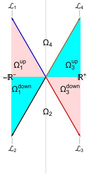
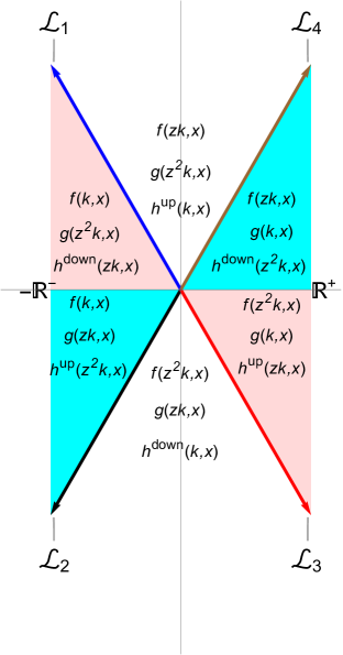
Figure 2.2: The complex $k$-plane divided into the six sectors $\Omega^{\text{\rm{up}}}_{1},$ $\Omega^{\text{\rm{down}}}_{1},$ $\Omega_{2},$ $\Omega^{\text{\rm{down}}}_{3},$ $\Omega^{\text{\rm{up}}}_{3},$ and $\Omega_{4}$ as shown on the left plot, and the $k$-domains of three basic solutions to (1.1) in each of the six regions, respectively, shown on the right plot.

We introduce the solution $h^{\text{\rm{down}}}(k,x)$ to (1.1) with the $k$-domain $\overline{\Omega_{2}}$ and the solution $h^{\text{\rm{up}}}(k,x)$ to (1.1) with the $k$-domain $\overline{\Omega_{4}}$ via

$$h^{\text{\rm{down}}}(k,x):=\left[\overline{f}(-z^{2}k^{\ast},x)^{\ast}\,;\,\overline{g}(-zk^{\ast},x)^{\ast}\right],\qquad x\in\mathbb{R},$$ (2.16)

$$h^{\text{\rm{up}}}(k,x):=\left[\overline{f}(-zk^{\ast},x)^{\ast}\,;\,\overline{g}(-z^{2}k^{\ast},x)^{\ast}\right],\qquad x\in\mathbb{R},$$ (2.17)

where the asterisk denotes complex conjugation and we recall that $\overline{\Omega_{2}}$ and $\overline{\Omega_{4}}$ are the closures of the sectors $\Omega_{2}$ and $\Omega_{4}$ defined in (2.7) and (2.9), respectively. We remark that, on the right-hand sides of (2.16) and (2.17), we have the $2$-Wronskians of the Jost solutions to the adjoint equation

$$\overline{\psi}^{\prime\prime\prime}(k,x)+\overline{Q}(x)\,\overline{\psi}^{\prime}(k,x)+\overline{P}(x)\,\overline{\psi}(k,x)=k^{3}\,\overline{\psi}(k,x),\qquad x\in\mathbb{R},$$ (2.18)

with

$$\overline{Q}(x):=Q(x)^{\ast},\quad\overline{P}(x):=Q^{\prime}(x)^{\ast}-P(x)^{\ast},\qquad x\in\mathbb{R}.$$

We emphasize that the asterisk denotes complex conjugation and the overbar in our notation does not denote complex conjugation but is used to denote the quantities related to the adjoint equation (2.18). We note that the $2$-Wronskian $\left[F(x);G(x)\right]$ of two functions $F(x)$ and $G(x)$ is defined as

$$\left[F(x)\,;G(x)\right]=F(x)\,G^{\prime}(x)-F^{\prime}(x)\,G(x).$$

The quantity $\overline{f}(k,x)$ appearing in (2.16) and (2.17) is the left Jost solution to (2.18) satisfying the asymptotics similar to (2.10), i.e.

$$\begin{cases}\overline{f}(k,x)=e^{kx}\left[1+o(1)\right],\qquad x\to+\infty,\\ \vskip 6.0pt plus 2.0pt minus 2.0pt\cr\overline{f}^{\prime}(k,x)=k\,e^{kx}\left[1+o(1)\right],\qquad x\to+\infty,\\ \vskip 6.0pt plus 2.0pt minus 2.0pt\cr\overline{f}^{\prime\prime}(k,x)=k^{2}\,e^{kx}\left[1+o(1)\right],\qquad x\to+\infty,\end{cases}$$

and $\overline{g}(k,x)$ appearing in (2.16) and (2.17) is the right Jost solution to (2.18) satisfying the asymptotics similar to (2.11), i.e.

$$\begin{cases}\overline{g}(k,x)=e^{kx}\left[1+o(1)\right],\qquad x\to-\infty,\\ \vskip 6.0pt plus 2.0pt minus 2.0pt\cr\overline{g}^{\prime}(k,x)=k\,e^{kx}\left[1+o(1)\right],\qquad x\to-\infty,\\ \vskip 6.0pt plus 2.0pt minus 2.0pt\cr\overline{g}^{\prime\prime}(k,x)=k^{2}\,e^{kx}\left[1+o(1)\right],\qquad x\to-\infty.\end{cases}$$

The spacial asymptotics of $h^{\text{\rm{down}}}(k,x)$ in its $k$-domain $\overline{\Omega_{2}}$ are known [30]. As $x\to+\infty$ we have

$$h^{\text{\rm{down}}}(k,x)=\begin{cases}\begin{aligned} z(1-&z)ke^{kx}\,T_{\text{\rm{l}}}(z^{2}k)^{-1}[1+o(1)]\\ &-z(1-z)ke^{z^{2}kx}M(k)\,T_{\text{\rm{l}}}(k)^{-1}[1+o(1)],\qquad k\in\mathcal{L}_{2},\end{aligned}\\ \vskip 6.0pt plus 2.0pt minus 2.0pt\cr z(1-z)ke^{kx}\,T_{\text{\rm{l}}}(z^{2}k)^{-1}[1+o(1)],\qquad k\in\Omega_{2},\\ \vskip 6.0pt plus 2.0pt minus 2.0pt\cr z(1-z)ke^{kx}\,T_{\text{\rm{l}}}(z^{2}k)^{-1}[1+o(1)],\qquad k\in\mathcal{L}_{3},\end{cases}$$ (2.19)

where we recall that $M(k)$ and $T_{\text{\rm{l}}}(k)$ are the left scattering coefficients appearing in (2.14). Similarly, as $x\to-\infty$ we have

$$h^{\text{\rm{down}}}(k,x)=\begin{cases}z(1-z)ke^{kx}\,T_{\text{\rm{r}}}(zk)^{-1}[1+o(1)],\qquad k\in\mathcal{L}_{2},\\ \vskip 6.0pt plus 2.0pt minus 2.0pt\cr z(1-z)ke^{kx}\,T_{\text{\rm{r}}}(zk)^{-1}[1+o(1)],\qquad k\in\Omega_{2},\\ \vskip 6.0pt plus 2.0pt minus 2.0pt\cr\begin{aligned} z(1-&z)ke^{kx}\,T_{\text{\rm{r}}}(zk)^{-1}[1+o(1)]\\ &-z(1-z)ke^{zkx}R(k)\,T_{\text{\rm{r}}}(k)^{-1}[1+o(1)],\qquad k\in\mathcal{L}_{3},\end{aligned}\end{cases}$$ (2.20)

where we recall that $R(k)$ and $T_{\text{\rm{r}}}(k)$ are the right scattering coefficients appearing in (2.15). In a similar manner, the spacial asymptotics of $h^{\text{\rm{up}}}(k,x)$ in its $k$-domain $\overline{\Omega_{4}}$ are known [30]. As $x\to+\infty$ we have

$$h^{\text{\rm{up}}}(k,x)=\begin{cases}\begin{aligned} -z(1-&z)ke^{kx}\,T_{\text{\rm{l}}}(zk)^{-1}[1+o(1)]\\ &+z(1-z)ke^{zkx}L(k)\,T_{\text{\rm{l}}}(k)^{-1}[1+o(1)],\qquad k\in\mathcal{L}_{1},\end{aligned}\\ \vskip 6.0pt plus 2.0pt minus 2.0pt\cr-z(1-z)ke^{kx}\,T_{\text{\rm{l}}}(zk)^{-1}[1+o(1)],\qquad k\in\Omega_{4},\\ \vskip 6.0pt plus 2.0pt minus 2.0pt\cr-z(1-z)ke^{kx}\,T_{\text{\rm{l}}}(zk)^{-1}[1+o(1)],\qquad k\in\mathcal{L}_{4},\end{cases}$$ (2.21)

where we recall that $L(k)$ is the left primary reflection coefficient appearing in (2.14). Similarly, as $x\to-\infty$ we have

$$h^{\text{\rm{up}}}(k,x)=\begin{cases}-z(1-z)ke^{kx}\,T_{\text{\rm{r}}}(z^{2}k)^{-1}[1+o(1)],\qquad k\in\mathcal{L}_{1},\\ \vskip 6.0pt plus 2.0pt minus 2.0pt\cr-z(1-z)ke^{kx}\,T_{\text{\rm{r}}}(z^{2}k)^{-1}[1+o(1)],\qquad k\in\Omega_{4},\\ \vskip 6.0pt plus 2.0pt minus 2.0pt\cr\begin{aligned} -z(1-&z)ke^{kx}\,T_{\text{\rm{r}}}(z^{2}k)^{-1}[1+o(1)]\\ &+z(1-z)ke^{z^{2}kx}N(k)\,T_{\text{\rm{r}}}(k)^{-1}[1+o(1)],\qquad k\in\mathcal{L}_{4},\end{aligned}\end{cases}$$ (2.22)

where we recall that $N(k)$ is the right secondary reflection coefficient appearing in (2.15).

Since (1.1) is a linear homogeneous ordinary differential equation, any constant multiple of a solution to (1.1) is also a solution. As seen from (2.19)–(2.22), it is convenient to let

$$m(k,x):=\displaystyle\frac{T_{\text{\rm{r}}}(zk)\,h^{\text{\rm{down}}}(k,x)}{z(1-z)k},\qquad k\in\overline{\Omega_{2}},\quad x\in\mathbb{R},$$ (2.23)

$$n(k,x):=\displaystyle\frac{T_{\text{\rm{r}}}(z^{2}k)\,h^{\text{\rm{up}}}(k,x)}{-z(1-z)k},\qquad k\in\overline{\Omega_{4}},\quad x\in\mathbb{R},$$ (2.24)

so that $m(k,x)$ and $n(k,x)$ remain solutions to (1.1) with the respective $k$-domains $\overline{\Omega_{2}}$ and $\overline{\Omega_{4}},$ but with simpler spacial asymptotics. As $x\to+\infty,$ with the help of (2.19) and (2.23) we obtain

$$m(k,x)=\begin{cases}\begin{aligned} e^{kx}&\,T_{\text{\rm{l}}}(z^{2}k)^{-1}\,T_{\text{\rm{r}}}(zk)[1+o(1)]\\ &-e^{z^{2}kx}M(k)\,T_{\text{\rm{l}}}(k)^{-1}\,T_{\text{\rm{r}}}(zk)[1+o(1)],\qquad k\in\mathcal{L}_{2},\end{aligned}\\ \vskip 6.0pt plus 2.0pt minus 2.0pt\cr e^{kx}\,T_{\text{\rm{l}}}(z^{2}k)^{-1}\,T_{\text{\rm{r}}}(zk)[1+o(1)],\qquad k\in\Omega_{2},\\ \vskip 6.0pt plus 2.0pt minus 2.0pt\cr e^{kx}\,T_{\text{\rm{l}}}(z^{2}k)^{-1}\,T_{\text{\rm{r}}}(zk)[1+o(1)],\qquad k\in\mathcal{L}_{3}.\end{cases}$$ (2.25)

As $x\to-\infty,$ with the help of (2.20) and (2.23), we have

$$m(k,x)=\begin{cases}e^{kx}[1+o(1)],\qquad k\in\mathcal{L}_{2},\\ \vskip 6.0pt plus 2.0pt minus 2.0pt\cr e^{kx}[1+o(1)],\qquad k\in\Omega_{2},\\ \vskip 6.0pt plus 2.0pt minus 2.0pt\cr e^{kx}[1+o(1)]-e^{zkx}R(k)\,T_{\text{\rm{r}}}(k)^{-1}\,T_{\text{\rm{r}}}(zk)[1+o(1)],\qquad k\in\mathcal{L}_{3}.\end{cases}$$ (2.26)

As $x\to+\infty$ we get

$$n(k,x)=\begin{cases}\begin{aligned} e^{kx}&\,T_{\text{\rm{l}}}(zk)^{-1}\,T_{\text{\rm{r}}}(z^{2}k)[1+o(1)]\\ &-e^{zkx}L(k)\,T_{\text{\rm{l}}}(k)^{-1}\,T_{\text{\rm{r}}}(z^{2}k)[1+o(1)],\qquad k\in\mathcal{L}_{1},\end{aligned}\\ \vskip 6.0pt plus 2.0pt minus 2.0pt\cr e^{kx}\,T_{\text{\rm{l}}}(zk)^{-1}\,T_{\text{\rm{r}}}(z^{2}k)[1+o(1)],\qquad k\in\Omega_{4},\\ \vskip 6.0pt plus 2.0pt minus 2.0pt\cr e^{kx}\,T_{\text{\rm{l}}}(zk)^{-1}\,T_{\text{\rm{r}}}(z^{2}k)[1+o(1)],\qquad k\in\mathcal{L}_{4}.\end{cases}$$ (2.27)

Similarly, as $x\to-\infty$ we have

$$n(k,x)=\begin{cases}e^{kx}[1+o(1)],\qquad k\in\mathcal{L}_{1},\\ \vskip 6.0pt plus 2.0pt minus 2.0pt\cr e^{kx}[1+o(1)],\qquad k\in\Omega_{4},\\ \vskip 6.0pt plus 2.0pt minus 2.0pt\cr e^{kx}[1+o(1)]-e^{z^{2}kx}N(k)\,T_{\text{\rm{r}}}(k)^{-1}\,T_{\text{\rm{r}}}(z^{2}k)[1+o(1)],\qquad k\in\mathcal{L}_{4}.\end{cases}$$ (2.28)

For each fixed $x\in\mathbb{R},$ we have [30] the large $k$-asymptotics

$$\begin{cases}m(k,x)=e^{kx}\left[1+O\left(\displaystyle\frac{1}{k}\right)\right],\qquad k\to\infty\text{\rm{ in }}\overline{\Omega_{2}},\\ \vskip 6.0pt plus 2.0pt minus 2.0pt\cr n(k,x)=e^{kx}\left[1+O\left(\displaystyle\frac{1}{k}\right)\right],\qquad k\to\infty\text{\rm{ in }}\overline{\Omega_{4}}.\end{cases}$$ (2.29)

In the reflectionless case, the spacial asymptotics of $m(k,x)$ and $n(k,x)$ are even simpler, and from (2.25)–(2.28) we obtain

$$m(k,x)=\begin{cases}e^{kx}\,T_{\text{\rm{l}}}(z^{2}k)^{-1}\,T_{\text{\rm{r}}}(zk)[1+o(1)],\qquad x\to+\infty,\quad k\in\overline{\Omega_{2}},\\ \vskip 6.0pt plus 2.0pt minus 2.0pt\cr e^{kx}[1+o(1)],\qquad x\to-\infty,\quad k\in\overline{\Omega_{2}},\end{cases}$$ (2.30)

$$n(k,x)=\begin{cases}e^{kx}\,T_{\text{\rm{l}}}(zk)^{-1}\,T_{\text{\rm{r}}}(z^{2}k)[1+o(1)],\qquad x\to+\infty,\quad k\in\overline{\Omega_{4}},\\ \vskip 6.0pt plus 2.0pt minus 2.0pt\cr e^{kx}[1+o(1)],\qquad x\to-\infty,\quad k\in\overline{\Omega_{4}}.\end{cases}$$ (2.31)

We refer to $f(k,x),$ $g(k,x),$ $h^{\text{\rm{down}}}(k,x),$ and $h^{\text{\rm{up}}}(k,x)$ as the four basic solutions to (1.1). With the help of (2.1), we can show that $\psi(zk,x)$ and $\psi(z^{2}k,x)$ are solutions to (1.1) whenever $\psi(k,x)$ is a solution to (1.1). In fact, the $k$-domain of $\psi(zk,x)$ is obtained from the $k$-domain of $\psi(k,x)$ by a clockwise rotation of $2\pi/3$ radians around the origin of the complex $k$-plane $\mathbb{C}.$ Similarly, the $k$-domain of $\psi(z^{2}k,x)$ is obtained from the $k$-domain of $\psi(k,x)$ by a clockwise rotation of $4\pi/3$ radians around the origin of the complex $k$-plane $\mathbb{C}.$ Thus, at every $k$-value in the complex plane, with the help of the four basic solutions $f(k,x),$ $g(k,x),$ $h^{\text{\rm{down}}}(k,x),$ and $h^{\text{\rm{up}}}(k,x),$ we can form three linearly independent solutions to (1.1).

In the right plot of Figure 2.2, we present three solutions to (1.1) at each $k$-value in the complex $k$-plane. As seen from the left plot of Figure 2.2, this is done by displaying a specific set of three solutions to (1.1) in each of the six closed sectors $\overline{\Omega_{1}^{\text{\rm{up}}}},$ $\overline{\Omega_{1}^{\text{\rm{down}}}},$ $\overline{\Omega_{2}},$ $\overline{\Omega_{3}^{\text{\rm{down}}}},$ $\overline{\Omega_{3}^{\text{\rm{up}}}},$ and $\overline{\Omega_{4}},$ respectively. We remark that $\Omega_{1}^{\text{\rm{up}}},$ $\Omega_{1}^{\text{\rm{down}}},$ $\Omega_{3}^{\text{\rm{down}}},$ and $\Omega_{3}^{\text{\rm{up}}}$ are the respective open sectors parametrized as

$$\Omega_{1}^{\text{\rm{up}}}:=\left\{k\in\mathbb{C}:\displaystyle\frac{2\pi}{3}<\arg[k]<\pi\right\},$$ (2.32)

$$\Omega_{1}^{\text{\rm{down}}}:=\left\{k\in\mathbb{C}:\pi<\arg[k]<\displaystyle\frac{4\pi}{3}\right\},$$ (2.33)

$$\Omega_{3}^{\text{\rm{down}}}:=\left\{k\in\mathbb{C}:-\displaystyle\frac{\pi}{3}<\arg[k]<0\right\},$$

$$\Omega_{3}^{\text{\rm{up}}}:=\left\{k\in\mathbb{C}:0<\arg[k]<\displaystyle\frac{\pi}{3}\right\}.$$

The closed sector $\overline{\Omega_{1}^{\text{\rm{up}}}}$ is the closure of $\Omega_{1}^{\text{\rm{up}}},$ and it is obtained from $\Omega_{1}^{\text{\rm{up}}}$ by including its upper boundary $\mathcal{L}_{1}$ and its lower boundary $-\mathbb{R}^{-}.$ We use $-\mathbb{R}^{-}$ to denote the directed half line given by

$$-\mathbb{R}^{-}:=\{k=-s:s\in[0,+\infty)\}.$$

Similarly, the closed sector $\overline{\Omega_{1}^{\text{\rm{down}}}}$ is the closure of $\Omega_{1}^{\text{\rm{down}}},$ and it is obtained from $\Omega_{1}^{\text{\rm{down}}}$ by including its upper boundary $-\mathbb{R}^{-}$ and its lower boundary $\mathcal{L}_{2}.$ The closed sector $\overline{\Omega_{3}^{\text{\rm{down}}}}$ is the closure of $\Omega_{3}^{\text{\rm{down}}},$ and it is obtained from $\Omega_{3}^{\text{\rm{down}}}$ by including its lower boundary $\mathcal{L}_{3}$ and its upper boundary $\mathbb{R}^{+},$ where $\mathbb{R}^{+}$ is the directed half line corresponding to the real interval $[0,+\infty)$ in the complex $k$-plane. Similarly, $\overline{\Omega_{3}^{\text{\rm{up}}}}$ is the closure of $\Omega_{3}^{\text{\rm{up}}},$ and it is obtained from $\Omega_{3}^{\text{\rm{up}}}$ by including its lower boundary $\mathbb{R}^{+}$ and its upper boundary $\mathcal{L}_{4}.$

We define the $3$-Wronskian of three functions $F(x),$ $G(x),$ and $H(x)$ as

$$\left[F(x);G(x);H(x)\right]:=\begin{vmatrix}F(x)&G(x)&H(x)\\ F^{\prime}(x)&G^{\prime}(x)&H^{\prime}(x)\\ F^{\prime\prime}(x)&G^{\prime\prime}(x)&H^{\prime\prime}(x)\end{vmatrix},$$

where we have the determinant of the relevant $3\times 3$ matrix on the right-hand side. Because the coefficient of $\psi^{\prime\prime}$ is zero in (1.1), the Wronskian of any three solutions to (1.1) at any particular $k$-value is zero if and only if those three solutions are linearly dependent. Furthermore, the Wronskian of those three solutions is independent of $x$ and its value can be evaluated at any particular $x$-value. For example, using their asymptotics as $x\to\pm\infty,$ we evaluate the $3$-Wronskian of $f(k,x),$ $g(zk,x),$ and $h^{\text{\rm{up}}}(z^{2}k,x)$ in $\overline{\Omega_{1}^{\text{\rm{down}}}}$ as

$$\left[f(k,x);g(zk,x);h^{\text{\rm{up}}}(z^{2}k,x)\right]=-9z^{2}k^{4}\,T_{\text{\rm{l}}}(k)^{-1}\,T_{\text{\rm{r}}}(zk)^{-1},\qquad k\in\overline{\Omega_{1}^{\text{\rm{down}}}}.$$ (2.34)

Similarly, using their asymptotics as $x\to\pm\infty,$ we evaluate the $3$-Wronskian of $f(k,x),$ $g(z^{2}k,x),$ and $h^{\text{\rm{down}}}(zk,x)$ in $\overline{\Omega_{1}^{\text{\rm{up}}}}$ as

$$\left[f(k,x);g(z^{2}k,x);h^{\text{\rm{down}}}(zk,x)\right]=-9zk^{4}\,T_{\text{\rm{l}}}(k)^{-1}\,T_{\text{\rm{r}}}(zk)^{-1},\qquad k\in\overline{\Omega_{1}^{\text{\rm{up}}}}.$$ (2.35)

Using (2.24) and (2.34) we have

$$\left[f(k,x);g(zk,x);n(z^{2}k,x)\right]=-3z(1-z)k^{3}\,T_{\text{\rm{l}}}(k)^{-1},\qquad k\in\overline{\Omega_{1}^{\text{\rm{down}}}},$$ (2.36)

and using (2.23) and (2.35) we get

$$\left[f(k,x);g(z^{2}k,x);m(zk,x)\right]=3(1-z^{2})k^{3}\,T_{\text{\rm{l}}}(k)^{-1},\qquad k\in\overline{\Omega_{1}^{\text{\rm{up}}}}.$$ (2.37)

Comparing (2.34) and (2.35) with (2.36) and (2.37), we see another advantage of using $m(k,x)$ and $n(k,x)$ instead of $h^{\text{\rm{down}}}(k,x)$ and $h^{\text{\rm{up}}}(k,x),$ respectively. This is because, by using (2.36) and (2.37), we can directly relate the bound-state poles the left transmission coefficient $T_{\text{\rm{l}}}(k)$ to the linear dependence of the three relevant solutions to (1.1) in the appropriate $k$-domain.

If the potentials $Q$ and $P$ appearing in (1.1) depend on the time parameter $t,$ then the Jost solutions $f(k,x)$ and $g(k,x)$ to (1.1) also depend on $t.$ In that case, the time evolutions of $f(k,x)$ and $g(k,x)$ are determined with the help of the linear operator $A$ given in (1.3). In fact, the time evolution of any solution $\psi(k,x)$ to (1.1) is determined by using the requirement [3, 4] that the quantity $\partial\psi(k,x)/\partial t-A\psi(k,x)$ is a solution to (1.1). This yields the time evolutions for the Jost solutions $f(k,x)$ and $g(k,x),$ and we have

$$\frac{\partial f(k,x)}{\partial t}-A\,f(k,x)=-9k^{5}f(k,x),\qquad k\in\overline{\Omega_{1}},\quad x\in\mathbb{R},$$ (2.38)

$$\frac{\partial g(k,x)}{\partial t}-A\,g(k,x)=-9k^{5}g(k,x),\qquad k\in\overline{\Omega_{3}},\quad x\in\mathbb{R}.$$ (2.39)

With the help of (2.14), (2.15), (2.38), and (2.39), we obtain the time evolutions of the scattering coefficients for (1.1) as

$$\begin{cases}T_{\text{\rm{l}}}(k)\mapsto T_{\text{\rm{l}}}(k),\qquad k\in\overline{\Omega_{1}},\\ \vskip 6.0pt plus 2.0pt minus 2.0pt\cr T_{\text{\rm{r}}}(k)\mapsto T_{\text{\rm{l}}}(k),\qquad k\in\overline{\Omega_{3}},\\ \vskip 6.0pt plus 2.0pt minus 2.0pt\cr L(k)\mapsto L(k)\,\exp\left(9(z^{2}-1)k^{5}t\right),\qquad k\in\mathcal{L}_{1},\\ \vskip 6.0pt plus 2.0pt minus 2.0pt\cr M(k)\mapsto M(k)\,\exp\left(9(z-1)k^{5}t\right),\qquad k\in\mathcal{L}_{2},\\ \vskip 6.0pt plus 2.0pt minus 2.0pt\cr R(k)\mapsto R(k)\,\exp\left(9(z^{2}-1)k^{5}t\right),\qquad k\in\mathcal{L}_{3},\\ \vskip 6.0pt plus 2.0pt minus 2.0pt\cr N(k)\mapsto N(k)\,\exp\left(9(z-1)k^{5}t\right),\qquad k\in\mathcal{L}_{4}.\end{cases}$$ (2.40)

As indicated in (2.40), the transmission coefficients do not change in time. On the other hand, the reflection coefficients at any time $t$ are obtained by the corresponding reflection coefficients at $t=0$ using the indicated multiplicative exponential factors in (2.40). For example, the value $L(k)$ at any time $t$ is obtained by multiplying the value of $L(k)$ at $t=0$ with the exponential factor $e^{9(z^{2}-1)k^{5}t}.$

3 The bound states and bound-state dependency constants

A bound-state solution to (1.1) is defined as a nontrivial solution which is square integrable in $x\in\mathbb{R}.$ If the bound state occurs at the $k$-value $k_{j}$ in the complex $k$-plane, then the number of linearly independent square-integrable solutions to (1.1) at $k=k_{j},$ i.e.

$$\psi^{\prime\prime\prime}+Q(x)\,\psi^{\prime}+P(x)\,\psi=k_{j}^{3}\,\psi,\qquad x\in\mathbb{R},$$ (3.1)

determines the multiplicity of the bound state at $k=k_{j}.$ If there is only one linearly independent bound-state solution at $k=k_{j},$ then the bound state at $k=k_{j}$ is simple. We recall that we suppress the $t$-dependence of the potentials $Q$ and $P$ and any quantities related to (3.1) in our notation.

Suppose that the complex constant $k_{j}$ is located in the open sector $\Omega_{1}^{\text{\rm{down}}}$ and that it corresponds to a bound state. Then, we have $T_{\text{\rm{l}}}(k_{j})^{-1}=0.$ From (LABEL:2.44a) we see that the three solutions $f(k_{j},x),$ $g(zk_{j},x),$ and $n(z^{2}k_{j},x)$ to (3.1) become linearly dependent. This allows us to express $f(k_{j},x)$ as a linear combination of $g(zk_{j},x)$ and $n(z^{2}k_{j},x)$ as

$$f(k_{j},x)=D(k_{j})\,g(zk_{j},x)+W(k_{j})\,n(z^{2}k_{j},x),\qquad x\in\mathbb{R},$$ (3.2)

for some complex constants $D(k_{j})$ and $W(k_{j}).$

Let us divide the open sector $\Omega_{1}^{\text{\rm{down}}}$ specified in (2.33) into two parts, the first of which is the sector with $\arg[k]\in(\pi,7\pi/6)$ and the second sector is described by using $\arg[k]\in[7\pi/6,4\pi/3).$ If the bound state at $k=k_{j}$ occurs when $\arg[k_{j}]\in(\pi,7\pi/6),$ then from (3.2) we get $D(k_{j})=0$ and hence (3.2) yields

$$f(k_{j},x)=W(k_{j})\,n(z^{2}k_{j},x),\qquad\arg[k_{j}]\in\left(\pi,\displaystyle\frac{7\pi}{6}\right),\quad x\in\mathbb{R},$$ (3.3)

where $W(k_{j})\neq 0$ and the complex constant $W(k_{j})$ corresponds to the dependency constant at the bound state with $k=k_{j}.$ On the other hand, if we have $\arg[k_{j}]\in[7\pi/6,4\pi/3),$ then from (3.2) we get $W(k_{j})=0$ and hence (3.2) yields

$$f(k_{j},x)=D(k_{j})\,g(zk_{j},x),\qquad\arg[k_{j}]\in\left[\displaystyle\frac{7\pi}{6},\displaystyle\frac{4\pi}{3}\right),\quad x\in\mathbb{R},$$ (3.4)

where $D(k_{j})\neq 0$ and the complex constant $D(k_{j})$ corresponds to the dependency constant at the bound state with $k=k_{j}.$

By using the following argument, we show how each of (3.3) and (3.4) follows from (3.2). When $k_{j}\in\Omega_{1}^{\text{\rm{down}}},$ the real and imaginary parts of the complex constant $k_{j}$ are both negative, i.e. we have

$$\text{Re}[k_{j}]<0,\quad\text{Im}[k_{j}]<0,\qquad k_{j}\in\Omega_{1}^{\text{\rm{down}}}.$$ (3.5)

Using (3.5) in the first line of (2.10) we see that $f(k_{j},x)$ decays exponentially as $x\to+\infty.$ Since $T_{\text{\rm{l}}}(k_{j})^{-1}=0,$ from the second line of the right-hand side of (2.14) it follows that $f(k_{j},x)$ also vanishes as $x\to-\infty.$ Since those decays are exponential, $f(k_{j},x)$ corresponds to a bound-state solution to (3.1). With the help of the first line of the right-hand side of (2.11), we get

$$g(zk_{j},x)=\text{exp}\left(\bigg{(}-\displaystyle\frac{1}{2}+i\,\displaystyle\frac{\sqrt{3}}{2}\bigg{)}\bigg{(}\text{Re}[k_{j}]+i\,\text{Im}[k_{j}]\bigg{)}x\right)\left[1+o(1)\right],\qquad x\to-\infty,$$ (3.6)

which yields

$$\left|g(zk_{j},x)\right|=\left(\text{exp}\bigg{(}-\displaystyle\frac{1}{2}\,\text{Re}[k_{j}]-\displaystyle\frac{\sqrt{3}}{2}\,\text{Im}[k_{j}]\bigg{)}x\right)\left[1+o(1)\right],\qquad x\to-\infty.$$ (3.7)

Using (3.5) on the right-hand side of (3.7), we see that $g(zk_{j},x)$ decays exponentially as $x\to-\infty.$ On the other hand, from the second line of the right-hand side of (2.15) we observe that

$$\left|g(zk_{j},x)\right|=\left|T_{\text{\rm{r}}}(zk_{j})^{-1}\right|\left(\text{exp}\bigg{(}-\displaystyle\frac{1}{2}\,\text{Re}[k_{j}]-\displaystyle\frac{\sqrt{3}}{2}\,\text{Im}[k_{j}]\bigg{)}x\right)\left[1+o(1)\right],\qquad x\to+\infty.$$ (3.8)

When $\arg[k_{j}]\in(\pi,7\pi/6),$ we see from (3.8) that $\left|g(zk_{j},x)\right|$ becomes unbounded as $x\to+\infty.$ On the other hand, when $\arg[k_{j}]\in[7\pi/6,4\pi/3),$ we see from (3.8) that $g(zk_{j},x)$ decays exponentially as $x\to+\infty.$ Hence, for (3.2) to hold we must have $D(k_{j})=0$ when $\arg[k_{j}]\in(\pi,7\pi/6).$ In a similar way, since $T_{\text{\rm{l}}}(k_{j})^{-1}=0,$ from the first line of the right-hand side of (2.31) it follows that $n(z^{2}k_{j},x)$ vanishes exponentially as $x\to+\infty.$ From the second line of the right-hand side of (2.31), we get

$$n(z^{2}k_{j},x)=\text{exp}\left(\bigg{(}-\displaystyle\frac{1}{2}-i\,\displaystyle\frac{\sqrt{3}}{2}\bigg{)}\bigg{(}\text{Re}[k_{j}]+i\,\text{Im}[k_{j}]\bigg{)}x\right)\left[1+o(1)\right],\qquad x\to+\infty,$$ (3.9)

which yields

$$\left|n(z^{2}k_{j},x)\right|=\left(\text{exp}\bigg{(}-\displaystyle\frac{1}{2}\,\text{Re}[k_{j}]+\displaystyle\frac{\sqrt{3}}{2}\,\text{Im}[k_{j}]\bigg{)}x\right)\left[1+o(1)\right],\qquad x\to+\infty.$$ (3.10)

From (3.10) we see that $n(z^{2}k_{j},x)$ decays exponentially as $x\to+\infty$ when $\arg[k_{j}]\in(\pi,7\pi/6).$ On the other hand, when $\arg[k_{j}]=7\pi/6,$ it follows from (3.10) that $n(z^{2}k_{j},x)$ remains bounded as $x\to+\infty$ but does not vanish as $x\to+\infty.$ When $\arg[k_{j}]\in(7\pi/6,4\pi/3),$ from (3.10) it follows that $\left|n(z^{2}k_{j},x)\right|$ becomes unbounded as $x\to+\infty$ and hence $n(z^{2}k_{j},x)$ does not vanish as $x\to+\infty.$ Thus, for (3.2) to hold we must have $W(k_{j})=0$ when $\arg[k_{j}]\in[7\pi/6,4\pi/3).$ This concludes the justification of (3.3) and (3.4).

Next, we determine the time evolutions of the dependency constants $W(k_{j})$ and $D(k_{j})$ appearing in (3.3) and (3.4), respectively. We first determine the time evolution of the dependency constant $W(k_{j}).$ In analogy with (2.38) and (2.39), we have the time evolution of the solution $n(k,x)$ given by

$$\frac{\partial}{\partial t}n(k,x)-A\,n(k,x)=-9k^{5}\,n(k,x),\qquad k\in\overline{\Omega_{1}^{\text{\rm{up}}}},\quad x\in\mathbb{R}.$$ (3.11)

From (2.38) and (3.11) we have

$$\frac{\partial f(k_{j},x)}{\partial t}-A\,f(k_{j},x)=-9k_{j}^{5}\,f(k_{j},x),\qquad x\in\mathbb{R},$$ (3.12)

$$\frac{\partial}{\partial t}n(z^{2}k_{j},x)-A\,n(z^{2}k_{j},x)=-9zk_{j}^{5}\,n(z^{2}k_{j},x),\qquad x\in\mathbb{R},$$ (3.13)

where we have used $z^{10}=z$ in (3.13). Using (3.3) in (3.12) we obtain

$$\frac{\partial}{\partial t}\left(W(k_{j})\,n(z^{2}k_{j},x)\right)-A\left(W(k_{j})\,n(z^{2}k_{j},x)\right)=-9k_{j}^{5}\,W(k_{j})\,n(z^{2}k_{j},x),\qquad x\in\mathbb{R}.$$ (3.14)

Taking the $t$-derivative of the first term on the left-hand side of (3.14), we get

$$\begin{split}\displaystyle\frac{\partial W(k_{j})}{\partial t}\,n(z^{2}k_{j},x)+W(k_{j})\,&\displaystyle\frac{\partial n(z^{2}k_{j},x)}{\partial t}-W(k_{j})\,A\,n(z^{2}k_{j},x)\\ &=-9k_{j}^{5}\,W(k_{j})\,n(z^{2}k_{j},x),\qquad x\in\mathbb{R}.\end{split}$$ (3.15)

Multiplying both sides of (3.13) by $W(k_{j})$ and subtracting the resulting equality from (3.15), we obtain

$$\frac{\partial W(k_{j})}{\partial t}\,n(z^{2}k_{j},x)=(-9k_{j}^{5}+9zk_{j}^{5})\,W(k_{j})\,n(z^{2}k_{j},x),\qquad x\in\mathbb{R},$$ (3.16)

which simplifies to

$$\frac{\partial W(k_{j})}{\partial t}=9(z-1)k_{j}^{5}\,W(k_{j}),\qquad x\in\mathbb{R}.$$ (3.17)

Thus, the time evolution of $W(k_{j})$ is given by

$$W(k_{j})=U(k_{j})\,e^{9(z-1)k_{j}^{5}t},\qquad\arg[k_{j}]\in(\pi,7\pi/6),$$ (3.18)

where $U(k_{j})$ is the dependency constant at $t=0.$ We refer to $U(k_{j})$ as the initial bound-state dependency constant at $k=k_{j}.$

Next, we determine the time evolution of the dependency constant $D(k_{j})$ appearing in (3.4). We again assume that we have a simple bound state at $k=k_{j}$ with $\arg[k_{j}]\in[7\pi/6,4\pi/3).$ From (2.38) and (2.39) we have

$$\frac{\partial g(zk_{j},x)}{\partial t}-A\,g(zk_{j},x)=-9z^{2}k_{j}^{5}\,g(zk_{j},x),\qquad x\in\mathbb{R},$$ (3.19)

where we have used $z^{5}=z^{2}$ in (3.19). Using (3.4) in (3.12) we get

$$\frac{\partial}{\partial t}\big{(}D(k_{j})\,g(zk_{j},x)\big{)}-A\,\big{(}D(k_{j})\,g(zk_{j},x)\big{)}=-9k_{j}^{5}\,D(k_{j})\,g(zk_{j},x),\qquad x\in\mathbb{R}.$$ (3.20)

By taking the $t$-derivative of the first term on the left-hand side of (3.20), we get

$$\frac{\partial D(k_{j})}{\partial t}\,g(zk_{j},x)+D(k_{j})\,\displaystyle\frac{\partial g(zk_{j},x)}{\partial t}-D(k_{j})\,A\,g(zk_{j},x)=-9k_{j}^{5}\,D(k_{j})\,g(zk_{j},x),\qquad x\in\mathbb{R}.$$ (3.21)

Multiplying both sides of (3.19) by $D(k_{j})$ and subtracting the resulting equality from (3.21), we obtain

$$\frac{\partial D(k_{j})}{\partial t}\,g(zk_{j},x)=\left(-9k_{j}^{5}+9z^{2}k_{j}^{5}\right)D(k_{j})\,g(zk_{j},x),\qquad x\in\mathbb{R},$$ (3.22)

which simplifies to

$$\frac{\partial D(k_{j})}{\partial t}=9(z^{2}-1)k_{j}^{5}\,D(k_{j}),\qquad x\in\mathbb{R}.$$ (3.23)

Thus, the time evolution of $D(k_{j})$ is given by

$$D(k_{j})=E(k_{j})\,e^{9(z^{2}-1)\,k_{j}^{5}\,t},\qquad\arg[k_{j}]\in[7\pi/6,4\pi/3),$$ (3.24)

where $E(k_{j})$ is the dependency constant at $t=0.$ We refer to $E(k_{j})$ as the initial dependency constant at the bound state at $k=k_{j}.$

A simple bound state at $k=k_{j}$ with $k_{j}\in\Omega_{1}^{\text{\rm{down}}}$ occurs when $T_{\text{\rm{l}}}(k)^{-1}$ has a simple zero at $k=k_{j}$ or equivalently when $T_{\text{\rm{l}}}(k)$ has a simple pole at $k=k_{j}.$ A double pole at $k=k_{j}$ for $T_{\text{\rm{l}}}(k)$ corresponds to a bound state at $k=k_{j}$ having multiplicity two. If the bound state at $k=k_{j}$ has multiplicity $m_{j},$ then instead of having a single bound-state dependency constant $W(k_{j})$ in (3.3) or $D(k_{j})$ in (3.4), we have $m_{j}$ bound-state dependency constants. We refer the reader to [5, 6, 7] for handling bound states with multiplicities and determining the corresponding dependency constants in the presence of bound states with multiplicities. We postpone further elaborations on the multiplicities of the bound states for (1.1) to a future paper.

Let us remark that a bound state can also be described with the help of a normalization constant instead of a dependency constant. For example, assume that $k_{j}$ in $\Omega_{1}^{\text{\rm{down}}}$ corresponds to a simple bound state pole of $T_{\text{\rm{l}}}(k).$ As seen from (3.3), as a bound-state wavefunction, we can use either $f(k_{j},x)$ or $n(z^{2}k_{j},x)$ when $\arg[k_{j}]\in\left(\pi,7\pi/6\right)$ and we can use either $f(k_{j},x)$ or $g(zk_{j},x)$ when $\arg[k_{j}]\in\left[7\pi/6,4\pi/3\right).$ Thus, when $\arg[k_{j}]\in\left(\pi,7\pi/6\right)$ the bound-state data set can be specified by using $k_{j}$ and $W(k_{j}),$ and when $\arg[k_{j}]\in\left[7\pi/6,4\pi/3\right)$ the bound-state data set can be specified by using $k_{j}$ and $D(k_{j}).$ Alternatively, we can introduce the left bound-state normalization constant $c_{\text{\rm{l}}}(k_{j})$ by using

$$c_{\text{\rm{l}}}(k_{j}):=\displaystyle\frac{1}{\sqrt{\displaystyle\int_{-\infty}^{\infty}dx\left|f(k_{j},x)\right|^{2}}},\qquad k_{j}\in\Omega_{1}^{\text{\rm{down}}},$$ (3.25)

so that the quantity $c_{\text{\rm{l}}}(k_{j})\,f(k_{j},x)$ is a normalized bound-state solution to (3.1). Instead of using the left bound-state normalization constant, we can alternatively use the right bound-state normalization constant $c_{\text{\rm{r}}}(k_{j})$ by letting

$$c_{\text{\rm{r}}}(k_{j}):=\begin{cases}\displaystyle\frac{1}{\sqrt{\displaystyle\int_{-\infty}^{\infty}dx\,n(z^{2}k_{j},x)}},\qquad\arg[k_{j}]\in\left(\pi,\displaystyle\frac{7\pi}{6}\right),\\ \vskip 6.0pt plus 2.0pt minus 2.0pt\cr\displaystyle\frac{1}{\sqrt{\displaystyle\int_{-\infty}^{\infty}dx\,g(zk_{j},x)}},\qquad\arg[k_{j}]\in\left[\displaystyle\frac{7\pi}{6},\displaystyle\frac{4\pi}{3}\right),\end{cases}$$ (3.26)

so that $c_{\text{\rm{r}}}(k_{j})\,n(z^{2}k_{j},x)$ is a normalized bound-state solution to (3.1) when $\arg[k_{j}]\in\left(\pi,7\pi/6\right)$ or that $c_{\text{\rm{r}}}(k_{j})\,g(zk_{j},x)$ is a normalized bound-state solution to (3.1) when $\arg[k_{j}]\in\left[7\pi/6,4\pi/3\right)$. From (3.3) and (3.4), for $x\in\mathbb{R}$ we have

$$\left|f(k_{j},x)\right|^{2}=\begin{cases}\left|W(k_{j})\right|^{2}\left|n(z^{2}k_{j},x)\right|^{2},\qquad\arg[k_{j}]\in\left(\pi,\displaystyle\frac{7\pi}{6}\right),\\ \vskip 6.0pt plus 2.0pt minus 2.0pt\cr\left|D(k_{j})\right|^{2}\left|g(zk_{j},x)\right|^{2},\qquad\arg[k_{j}]\in\left[\displaystyle\frac{7\pi}{6},\displaystyle\frac{4\pi}{3}\right).\end{cases}$$ (3.27)

Integrating both sides of (3.27) on $x\in\mathbb{R}$ and using (3.25) and (3.26), we obtain

$$\frac{1}{c_{\text{\rm{l}}}(k_{j})^{2}}=\begin{cases}\left|W(k_{j})\right|^{2}\displaystyle\frac{1}{c_{\text{\rm{r}}}(k_{j})^{2}},\qquad\arg[k_{j}]\in\left(\pi,\displaystyle\frac{7\pi}{6}\right),\\ \vskip 6.0pt plus 2.0pt minus 2.0pt\cr\left|D(k_{j})\right|^{2}\displaystyle\frac{1}{c_{\text{\rm{r}}}(k_{j})^{2}},\qquad\arg[k_{j}]\in\left[\displaystyle\frac{7\pi}{6},\displaystyle\frac{4\pi}{3}\right).\end{cases}$$ (3.28)

Since $c_{\text{\rm{l}}}(k_{j})$ and $c_{\text{\rm{r}}}(k_{j})$ are chosen as positive constants, from (3.28) we get

$$\frac{c_{\text{\rm{r}}}(k_{j})}{c_{\text{\rm{l}}}(k_{j})}=\begin{cases}\left|W(k_{j})\right|,\qquad\arg[k_{j}]\in\left(\pi,\displaystyle\frac{7\pi}{6}\right),\\ \vskip 6.0pt plus 2.0pt minus 2.0pt\cr\left|D(k_{j})\right|,\qquad\arg[k_{j}]\in\left[\displaystyle\frac{7\pi}{6},\displaystyle\frac{4\pi}{3}\right),\end{cases}$$

which is the analog of the second equality in (18) of [8]. It is possible to relate each of the dependency constants $W(k_{j})$ and $D(k_{j})$ to the normalization constants $c_{\text{\rm{l}}}(k_{j})$ and $c_{\text{\rm{r}}}(k_{j})$ by using the residue of $T_{\text{\rm{l}}}(k)$ at the bound-state pole with $k=k_{j}.$ This can be achieved by expanding both sides of (LABEL:2.44a) at $k=k_{j}$ and by equating the corresponding coefficient of $(k-k_{j})$ on both sides of the expansion.

We remark that the sectors $\Omega_{1}^{\text{\rm{up}}}$ and $\Omega_{1}^{\text{\rm{down}}}$ defined in (2.32) and (2.33), respectively, are symmetrically located with respect to the directed half line $-\mathbb{R}^{-}.$ There is a one-to-one correspondence between the point $k_{j}\in\Omega_{1}^{\text{\rm{down}}}$ and the point $k_{j}^{\ast}\in\Omega_{1}^{\text{\rm{up}}},$ where we recall that an asterisk denotes complex conjugation. Thus, if there is a bound state occurring at a $k$-value in the sector $\Omega_{1}^{\text{\rm{up}}},$ without loss of generality we can assume that it occurs at $k=k_{j}^{\ast}$ with $k_{j}\in\Omega_{1}^{\text{\rm{down}}}.$ In that case, let us determine the counterparts of (3.18) and (3.24). By proceeding in a manner similar to the steps given in (3.2)–(3.24), we introduce the bound-state dependency constants $W(k_{j}^{\ast})$ and $D(k_{j}^{\ast})$ as the complex constants satisfying for $x\in\mathbb{R}$

$$f(k_{j}^{\ast},x)=\begin{cases}W(k_{j}^{\ast})\,n(zk_{j}^{\ast},x),\qquad\arg[k_{j}^{\ast}]\in\left(\displaystyle\frac{5\pi}{6},\pi\right),\\ \vskip 6.0pt plus 2.0pt minus 2.0pt\cr D(k_{j}^{\ast})\,g(z^{2}k_{j}^{\ast},x),\qquad\arg[k_{j}^{\ast}]\in\left(\displaystyle\frac{2\pi}{3},\displaystyle\frac{5\pi}{6}\right].\end{cases}$$

The time evolution of $W(k_{j}^{\ast})$ and $D(k_{j}^{\ast})$ each is respectively given by

$$\begin{cases}W(k_{j}^{\ast})=U(k_{j}^{\ast})\,e^{9(z^{2}-1)\,(k_{j}^{\ast})^{5}\,t},\qquad\arg[k_{j}^{\ast}]\in\left(\displaystyle\frac{5\pi}{6},\pi\right),\\ \vskip 6.0pt plus 2.0pt minus 2.0pt\cr D(k_{j}^{\ast})=E(k_{j}^{\ast})\,e^{9(z-1)\,(k_{j}^{\ast})^{5}\,t},\qquad\arg[k_{j}^{\ast}]\in\left(\displaystyle\frac{2\pi}{3},\displaystyle\frac{5\pi}{6}\right],\end{cases}$$ (3.29)

where $U(k_{j}^{\ast})$ and $E(k_{j}^{\ast})$ are the respective dependency constants at $t=0.$ We refer to them as the initial bound-state dependency constants at $k=k_{j}^{\ast}.$

Let us now consider the special case when the potentials $Q$ and $P$ appearing in (1.1) are real valued. In that case, if we have a simple bound state at $k=k_{j}$ with $k_{j}\in\Omega_{1}^{\text{\rm{down}}}$ and also a simple bound state at $k=k_{j}^{\ast}$ with $k_{j}^{\ast}\in\Omega_{1}^{\text{\rm{up}}},$ then we have

$$\begin{cases}W(k_{j}^{\ast})=W(k_{j})^{\ast},\quad U(k_{j}^{\ast})=U(k_{j})^{\ast},\qquad\arg[k_{j}^{\ast}]\in\left(\displaystyle\frac{5\pi}{6},\pi\right),\\ \vskip 6.0pt plus 2.0pt minus 2.0pt\cr D(k_{j}^{\ast})=D(k_{j})^{\ast},\quad E(k_{j}^{\ast})=E(k_{j})^{\ast},\qquad\arg[k_{j}^{\ast}]\in\left(\displaystyle\frac{2\pi}{3},\displaystyle\frac{5\pi}{6}\right].\end{cases}$$ (3.30)

The proof of (3.30) can be given as follows. When the potentials $Q$ and $P$ in (3.1) are real valued, by taking the complex conjugate of both sides of (3.1) we get

$$\psi^{\prime\prime\prime}(k_{j},x)^{\ast}+Q(x)\,\psi^{\prime}(k_{j},x)^{\ast}+P(x)\,\psi(k_{j},x)^{\ast}=(k_{j}^{3})^{\ast}\,\psi(k_{j},x)^{\ast},\qquad x\in\mathbb{R}.$$ (3.31)

On the other hand, by replacing $k_{j}$ by $k_{j}^{\ast},$ from (3.1) we obtain

$$\psi^{\prime\prime\prime}(k_{j}^{\ast},x)+Q(x)\,\psi^{\prime}(k_{j}^{\ast},x)+P(x)\,\psi(k_{j}^{\ast},x)=(k_{j}^{\ast})^{3}\,\psi(k_{j}^{\ast},x),\qquad x\in\mathbb{R}.$$ (3.32)

Comparing (3.31) and (3.32), we see that $f(k_{j},x)^{\ast}$ and $f(k_{j}^{\ast},x)$ satisfy the same differential equation. From (2.10) it follows that $f(k_{j},x)^{\ast}$ and $f(k_{j}^{\ast},x)$ satisfy the same asymptotics as $x\to+\infty$ obtained from (2.10) by taking the complex conjugate of the right-hand side of (2.10). Because of the uniqueness of the solution to (3.31) with the aforementioned asymptotics as $x\to+\infty,$ we have

$$f(k_{j}^{\ast},x)=f(k_{j},x)^{\ast},\qquad x\in\mathbb{R}.$$

A similar argument yields

$$n(zk_{j}^{\ast},x)=n(z^{2}k_{j},x)^{\ast},\qquad x\in\mathbb{R},$$ (3.33)

$$g(z^{2}k_{j}^{\ast},x)=g(zk_{j},x)^{\ast},\qquad x\in\mathbb{R}.$$ (3.34)

By taking the complex conjugate of both sides of (3.3) and (3.4), for $x\in\mathbb{R}$ we have

$$f(k_{j},x)^{\ast}:=\begin{cases}W(k_{j})^{\ast}\,n(z^{2}k_{j},x)^{\ast},\qquad\arg[k_{j}]\in\left(\pi,\displaystyle\frac{7\pi}{6}\right),\\ \vskip 6.0pt plus 2.0pt minus 2.0pt\cr D(k_{j})^{\ast}\,g(zk_{j},x)^{\ast},\qquad\arg[k_{j}]\in\left[\displaystyle\frac{7\pi}{6},\displaystyle\frac{4\pi}{3}\right).\end{cases}$$ (3.35)

Comparing (3.29) and (3.35), with the help of (3.33) and (3.34), we conclude that the first equalities in both lines of the right-hand side of (3.30) hold. Since those first equalities hold for all $t\in\mathbb{R},$ those equalities also hold at $t=0.$ Hence, the second equalities in both lines of the right-hand side of (3.30) also hold.

4 The Riemann–Hilbert problem in the reflectionless case

The inverse scattering problem for (1.1) consists of the recovery of the potentials $Q$ and $P$ from an appropriate scattering data set. Such a data set consists of the scattering coefficients for (1.1) and the bound-state information. In this section we consider the inverse scattering problem for (1.1) in the reflectionless case, i.e. in the special case when the reflection coefficients $L(k),$ $M(k),$ $R(k),$ $N(k)$ appearing in (2.14) and (2.15) are all zero in their respective domains.

In terms of the four basic solutions $f(k,x),$ $g(k,x),$ $h^{\text{\rm{down}}}(k,x),$ and $h^{\text{\rm{up}}}(k,x)$ appearing in (2.14), (2.15), (2.16), and (2.17), respectively, we introduce the two functions $\Phi_{+}(k,x)$ and $\Phi_{-}(k,x)$ by letting

$$\Phi_{+}(k,x):=\begin{cases}T_{\text{\rm{l}}}(k)\,f(k,x),\qquad k\in\overline{\Omega_{1}},\\ \vskip 6.0pt plus 2.0pt minus 2.0pt\cr\displaystyle\frac{T_{\text{\rm{r}}}(zk)\,h^{\text{\rm{down}}}(k,x)}{z(1-z)k},\qquad k\in\overline{\Omega_{2}},\end{cases}$$ (4.1)

$$\Phi_{-}(k,x):=\begin{cases}g(k,x),\qquad k\in\overline{\Omega_{3}},\\ \vskip 6.0pt plus 2.0pt minus 2.0pt\cr\displaystyle\frac{T_{\text{\rm{r}}}(z^{2}k)\,h^{\text{\rm{up}}}(k,x)}{-z(1-z)k},\qquad k\in\overline{\Omega_{4}},\end{cases}$$ (4.2)

where we recall that $T_{\text{\rm{l}}}(k)$ and $T_{\text{\rm{r}}}(k)$ are the left and right transmission coefficients appearing in (2.14) and (2.15), respectively. With the help of (2.23) and (2.24), we can express (4.1) and (4.2), respectively, as

$$\Phi_{+}(k,x):=\begin{cases}T_{\text{\rm{l}}}(k)\,f(k,x),\qquad k\in\overline{\Omega_{1}},\\ \vskip 6.0pt plus 2.0pt minus 2.0pt\cr m(k,x),\qquad k\in\overline{\Omega_{2}},\end{cases}$$ (4.3)

$$\Phi_{-}(k,x):=\begin{cases}g(k,x),\qquad k\in\overline{\Omega_{3}},\\ \vskip 6.0pt plus 2.0pt minus 2.0pt\cr n(k,x),\qquad k\in\overline{\Omega_{4}}.\end{cases}$$ (4.4)

In terms of the directed half lines $\mathcal{L}_{1}$ in (2.2) and $\mathcal{L}_{3}$ in (2.4), we define the directed full line $\mathcal{L}$ by letting $\mathcal{L}:=\mathcal{L}_{1}\cup(-\mathcal{L}_{3})$ so that $\mathcal{L}$ divides the complex $k$-plane into the open left-half complex plane $\mathcal{P}^{+}$ and the open right-half complex plane $\mathcal{P}^{-},$ as shown in the right plot of Figure 4.1. We can parametrize $\mathcal{L}$ as

$$\mathcal{L}:=\{k\in\mathbb{C}:k=zs\text{\rm{ for }}s\in(-\infty,+\infty)\}.$$

We refer to $\mathcal{P}^{+}$ as the plus region and we use $\overline{\mathcal{P}^{+}}$ to denote its closure, i.e. we let $\overline{\mathcal{P}^{+}}:=\mathcal{P}^{+}\cup\mathcal{L}.$ Similarly, we refer to $\mathcal{P}^{-}$ as the minus region and we use $\overline{\mathcal{P}^{-}}$ to denote its closure, i.e. we let $\overline{\mathcal{P}^{-}}:=\mathcal{P}^{-}\cup\mathcal{L}.$ We assume that the left transmission coefficient $T_{\text{\rm{l}}}(k)$ does not have any poles when $k\in\mathcal{L}_{1}\cup\mathcal{L}_{2}.$ Similarly, we assume that the right transmission coefficient $T_{\text{\rm{r}}}(k)$ does not have any poles when $k\in\mathcal{L}_{3}\cup\mathcal{L}_{4}.$ It is known [30] that the four basic solutions $f(k,x),$ $g(k,x),$ $h^{\text{\rm{down}}}(k,x),$ and $h^{\text{\rm{up}}}(k,x)$ are analytic in $k$ in the interior of their respective $k$-domains and are continuous in $k$ in their $k$-domains. Furthermore, when the secondary left reflection coefficient $M(k)$ appearing in (2.14) vanishes for $k\in\mathcal{L}_{2},$ we have

$$T_{\text{\rm{l}}}(k)\,f(k,x)=\displaystyle\frac{T_{\text{\rm{r}}}(zk)\,h^{\text{\rm{down}}}(k,x)}{z(1-z)k},\qquad k\in\mathcal{L}_{2}.$$

Similarly, when the secondary right reflection coefficient $N(k)$ appearing in (2.15) vanishes for $k\in\mathcal{L}_{4},$ we have

$$g(k,x)=\displaystyle\frac{T_{\text{\rm{r}}}(z^{2}k)\,h^{\text{\rm{up}}}(k,x)}{-z(1-z)k},\qquad k\in\mathcal{L}_{4}.$$

Thus, $\Phi_{+}(k,x)$ defined in (4.1) is meromorphic in $k\in\mathcal{P}^{+},$ and is continuous in $k\in\overline{\mathcal{P}^{+}}$ except perhaps at the poles of the transmission coefficient $T_{\text{\rm{l}}}(k)$ in $\Omega_{1}$ and the poles of $T_{\text{\rm{r}}}(zk)$ in $\Omega_{2}.$ It is possible that some of those poles are offset by the zeros of $f(k,x)$ and $h^{\text{\rm{down}}}(k,x),$ respectively. Using (2.12), (2.29), and the known [30] large $k$-asymptotics of the transmission coefficients, we have the large $k$-asymptotics of $\Phi_{+}(k,x)$ given by

$$\Phi_{+}(k,x)=e^{kx}\left[1+O\left(\displaystyle\frac{1}{k}\right)\right],\qquad k\to\infty\text{\rm{ in }}\overline{\mathcal{P}^{+}}.$$ (4.5)

We refer to $\Phi_{+}(k,x)$ as the plus function. We remark that it is customary to use the term plus function when that function is analytic in the plus region. We find it convenient to refer to $\Phi_{+}(k,x)$ as a plus function even though it is meromorphic rather than analytic in the plus region $\mathcal{P}^{+}.$

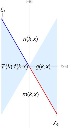
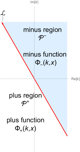
Figure 4.1: The $k$-domains of $T_{\text{\rm{l}}}(k)f(k,x),$ $m(k,x),$ $g(k,x),$ and $n(k,x),$ respectively, are shown on the left plot. The right plot shows the plus and minus regions in the complex $k$-plane separated by the directed full line $\mathcal{L},$ as well as the plus and minus functions in their respective $k$-domains.

In a similar manner, we establish that the function $\Phi_{-}(k,x)$ defined in (4.2) is meromorphic in $k\in\mathcal{P}^{-},$ is continuous in $k\in\overline{\mathcal{P}^{-}}$ except perhaps for the poles of the transmission coefficient of $T_{\text{\rm{r}}}(z^{2}k)$ in $\Omega_{4}.$ It is possible that some of the poles of $T_{\text{\rm{r}}}(z^{2}k)$ in $\Omega_{4}$ are offset by the zeros of $h^{\text{\rm{up}}}(k,x).$ Using (2.13), (2.29), and the known [30] large $k$-asymptotics of $T_{\text{\rm{r}}}(k)$ in its $k$-domain, we have the large $k$-asymptotics of $\Phi_{-}(k,x)$ given by

$$\Phi_{-}(k,x)=e^{kx}\left[1+O\left(\displaystyle\frac{1}{k}\right)\right],\qquad k\to\infty\text{\rm{ in }}\overline{\mathcal{P}^{-}}.$$ (4.6)

We remark that we refer to $\Phi_{-}(k,x)$ as the minus function even though $\Phi_{-}(k,x)$ is meromorphic and not necessarily analytic in the minus region $\mathcal{P}^{-}.$

Since the $k$-domain of $\Phi_{+}(k,x)$ is $\overline{\mathcal{P}^{+}}$ and the $k$-domain of $\Phi_{-}(k,x)$ is $\overline{\mathcal{P}^{-},}$ the common $k$-domain of $\Phi_{+}(k,x)$ and $\Phi_{-}(k,x)$ is the directed full line $\mathcal{L},$ and in fact in the reflectionless case those two functions agree [30] on $\mathcal{L}.$ Thus, we have

$$\Phi_{+}(k,x)=\Phi_{-}(k,x),\qquad k\in\mathcal{L}.$$ (4.7)

We view (4.7) as our Riemann–Hilbert problem as follows. As our input, we are given the transmission coefficients $T_{\text{\rm{l}}}(k)$ and $T_{\text{\rm{r}}}(k)$ in their respective $k$-domains $\overline{\Omega_{1}}$ and $\overline{\Omega_{3}}.$ We know that the reflection coefficients are all zero. In the reflectionless case, the right transmission coefficient $T_{\text{\rm{r}}}(k)$ is related [30] to the left transmission coefficient $T_{\text{\rm{l}}}(k)$ as

$$T_{\text{\rm{r}}}(z^{2}k)=T_{\text{\rm{l}}}(k)\,T_{\text{\rm{l}}}(zk),\qquad k\in\overline{\Omega_{1}},$$ (4.8)

and hence it is sufficient to specify only the left transmission coefficient $T_{\text{\rm{l}}}(k)$ in our input data set. Our input data set also contains a dependency constant for each pole of $T_{\text{\rm{l}}}(k)$ in $\Omega_{1}.$ In case of a pole with a multiplicity, the number of dependency constants for that pole must match the multiplicity of the pole. However, in this paper we only deal with simple bound states.

With the given input data set, for each fixed $x\in\mathbb{R},$ we solve (4.7) to determine $\Phi_{+}(k,x)$ in $\overline{\mathcal{P}^{+}}$ and $\Phi_{-}(k,x)$ in $\overline{\mathcal{P}^{-}}$ in such a way that the large $k$-asymptotics stated in (4.5) and (4.6) hold. Once we obtain $\Phi_{+}(k,x)$ and $\Phi_{-}(k,x)$ in their respective $k$-domains $\overline{\mathcal{P}^{+}}$ and $\overline{\mathcal{P}^{-}},$ as seen from (4.1) and (4.2), we can recover the four basic solutions $f(k,x),$ $g(k,x),$ $h^{\text{\rm{down}}}(k,x),$ and $h^{\text{\rm{up}}}(k,x)$ in their respective $k$-domains $\overline{\Omega_{1}},$ $\overline{\Omega_{2}},$ $\overline{\Omega_{3}},$ $\overline{\Omega_{4}}.$ Having those four basic solutions at hand, we can use them in their respective $k$-domains and we can recover the two potentials $Q(x)$ and $P(x).$ For example, we can recover $Q(x)$ and $P(x)$ by using either the left Jost solution $f(k,x)$ obtained in $k\in\Omega_{1}$ or the right Jost solution $g(k,x)$ obtained in $k\in\Omega_{3}$ with the help of the large $k$-asymptotics of those solutions. For example, the determination of $Q(x)$ and $P(x)$ from $f(k,x)$ can be achieved as follows. It is known [30] that we have the asymptotic expansion

$$f(k,x)=e^{kx}\left[1+\displaystyle\frac{u_{1}(x)}{k}+\displaystyle\frac{u_{2}(x)}{k^{2}}+O\left(\displaystyle\frac{1}{k^{3}}\right)\right],\qquad k\to\infty\text{\rm{ in }}\overline{\Omega_{1}},\quad x\in\mathbb{R},$$ (4.9)

where we have defined

$$u_{1}(x):=\displaystyle\frac{1}{3}\int_{x}^{\infty}dy\,Q(y),\qquad x\in\mathbb{R},$$ (4.10)

$$u_{2}(x):=-\displaystyle\frac{1}{3}\int_{x}^{\infty}dy\left[Q^{\prime}(y)-P(y)\right]+\displaystyle\frac{1}{18}\left[\int_{x}^{\infty}dy\,Q(y)\right]^{2},\qquad x\in\mathbb{R}.$$ (4.11)

With the help of (4.10) and (4.11), the potentials $Q(x)$ and $P(x)$ can be recovered from $u_{1}(x)$ and $u_{2}(x)$ as

$$Q(x)=-3\,\displaystyle\frac{du_{1}(x)}{dx},\qquad x\in\mathbb{R},$$ (4.12)

$$P(x)=3\left[u_{1}(x)\,\displaystyle\frac{du_{1}(x)}{dx}-\displaystyle\frac{d^{2}u_{1}(x)}{dx^{2}}-\displaystyle\frac{du_{2}(x)}{dx}\right],\qquad x\in\mathbb{R}.$$ (4.13)

Alternatively, we can recover the potentials $Q(x)$ and $P(x)$ from the right Jost solution $g(k,x)$ as follows. It is known [30] that we have the asymptotic expansion

$$g(k,x)=e^{kx}\left[1+\displaystyle\frac{v_{1}(x)}{k}+\displaystyle\frac{v_{2}(x)}{k^{2}}+O\left(\displaystyle\frac{1}{k^{3}}\right)\right],\qquad k\to\infty\text{\rm{ in }}\overline{\Omega_{4}},$$

where we have defined

$$v_{1}(x):=-\displaystyle\frac{1}{3}\int_{-\infty}^{x}dy\,Q(y),\qquad x\in\mathbb{R},$$ (4.14)

$$v_{2}(x):=\displaystyle\frac{1}{3}\int_{-\infty}^{x}dy\left[Q^{\prime}(y)-P(y)\right]+\displaystyle\frac{1}{18}\left[\int_{-\infty}^{x}dy\,Q(y)\right]^{2},\qquad x\in\mathbb{R}.$$ (4.15)

With the help of (4.14) and (4.15), we can recover the potentials $Q(x)$ and $P(x)$ from $v_{1}(x)$ and $v_{2}(x)$ as

$$Q(x)=-3\,\displaystyle\frac{dv_{1}(x)}{dx},\qquad x\in\mathbb{R},$$

$$P(x)=3\left[v_{1}(x)\,\displaystyle\frac{dv_{1}(x)}{dx}-\displaystyle\frac{d^{2}v_{1}(x)}{dx^{2}}-\displaystyle\frac{dv_{2}(x)}{dx}\right],\qquad x\in\mathbb{R}.$$

We recall that we suppress the dependence on the parameter $t$ in our notation. The procedure outlined above holds regardless of whether the potentials $Q$ and $P$ contain the time parameter $t.$ The parameter $t$ in the input data set only appears in the time evolutions of the bound-state dependency constants. For example, if the left transmission coefficient $T_{\text{\rm{l}}}(k)$ has a simple pole at $k=k_{j}$ in $\Omega_{1}^{\text{\rm{down}}},$ then the corresponding bound-state dependency constant $D(k_{j})$ evolves in time as in (3.24). If the left transmission coefficient $T_{\text{\rm{l}}}(k)$ has a simple pole at $k=k_{j}^{\ast}$ in $\Omega_{1}^{\text{\rm{up}}},$ then the corresponding bound-state dependency constant $D(k_{j}^{\ast})$ evolves in time as in the second line of (3.29).

5 Soliton solutions

In this section we present some explicit solutions to the system (1.6) and its two special cases given in (1.10). This is done by solving the inverse scattering problem for (1.1) explicitly with the appropriate input data set in the reflectionless case. We recall that we suppress the appearance of the time parameter $t$ in the arguments of the functions we use.

In the first example below we assume that our input data set contains the left transmission coefficient $T_{\text{\rm{l}}}(k)$ with $\mathbf{N}$ simple poles occurring at $k=k_{j}$ for $1\leq j\leq\mathbf{N},$ all located in the sector $\arg[k]\in[7\pi/6,4\pi/3).$ Our input data set is given by $\{k_{j},E(k_{j})\}_{j=1}^{\mathbf{N}},$ where $E(k_{j})$ is the initial bound-state dependency constant at $k=k_{j}$ appearing in (3.24). In case the simple poles $k_{j}$ occur in the sector $\arg[k]\in(\pi,7\pi/6),$ the example can be modified so that one can instead use the input data set $\{k_{j},U(k_{j})\}_{j=1}^{\mathbf{N}},$ where we recall that $U(k_{j})$ is the initial bound-state dependency constant at $k=k_{j}$ appearing in (3.18).

Example 5.1.

In this example, we construct the $\mathbf{N}$-soliton solution to (1.6) by solving the inverse scattering problem for (1.1) in the reflectionless case. Our input data set consists of a transmission coefficient and the associated bound-state dependency constants. We choose the left transmission coefficient $T_{\text{\rm{l}}}(k)$ as

$$T_{\text{\rm{l}}}(k)=\displaystyle\frac{F(k)}{G(k)},\qquad k\in\overline{\Omega_{1}},$$ (5.1)

where the scalar quantities $F(k)$ and $G(k)$ are defined as

$$F(k):=\displaystyle\prod_{j=1}^{\mathbf{N}}(k+k_{j}^{\ast}),\quad G(k):=\displaystyle\prod_{j=1}^{\mathbf{N}}(k-k_{j}).$$ (5.2)

In (5.2), $\mathbf{N}$ is a fixed positive integer and the complex constants $k_{j}$ are distinct and all occur in the sector $\arg[k]\in[7\pi/6,4\pi/3).$ We assume that the right transmission coefficient $T_{\text{\rm{r}}}(k)$ is given by reciprocal of $T_{\text{\rm{l}}}(k),$ i.e. we have

$$T_{\text{\rm{r}}}(k)=\displaystyle\frac{G(k)}{F(k)},\qquad k\in\overline{\Omega_{3}}.$$ (5.3)

We remark that (5.1) and (5.3) are compatible with the constraint (4.8). Our Riemann–Hilbert problem (4.7) with the large $k$-asymptotics in (4.5) and (4.6) can be solved by multiplying both sides of (4.7) by $e^{-kx}\,G(k).$ From (4.7) we get

$$e^{-kx}\,G(k)\,\Phi_{+}(k,x)=e^{-kx}\,G(k)\,\Phi_{-}(k,x),\qquad k\in\mathcal{L}.$$ (5.4)

The left-hand side of (5.4) has an analytic extension from $k\in\mathcal{L}$ to the plus region $\mathcal{P}^{+}$ and that the right-hand side of (5.4) has an analytic extension from $k\in\mathcal{L}$ to the minus region $\mathcal{P}^{-}.$ Using the large $k$-asymptotics given in (4.5) and (4.6), with the help of a generalization of the Liouville theorem [28], we conclude that each side of (5.4) is entire and equal to a monic polynomial in $k$ of degree $\mathbf{N}.$ We define $V(k)$ as the row vector with $\mathbf{N}$ components given by

$$V(k):=\begin{bmatrix}k^{\mathbf{N}-1}&k^{\mathbf{N}-2}&\cdots&k&1\end{bmatrix},\qquad k\in\mathbb{C}.$$ (5.5)

We use $\mathbf{A}(x)$ to denote the column vector with $\mathbf{N}$ components, which is given by

$$\mathbf{A}(x):=\begin{bmatrix}A_{\mathbf{N}-1}(x)\\ A_{\mathbf{N}-2}(x)\\ \vdots\\ A_{1}(x)\\ A_{0}(x)\end{bmatrix},\qquad x\in\mathbb{R},$$ (5.6)

where $A_{j}(x)$ is a scalar-valued function of $x\in\mathbb{R}$ for $0\leq j\leq\mathbf{N}-1.$ Thus, each side of (5.4) is equal to the monic polynomial $[k^{\mathbf{N}}+V(k)\,\mathbf{A}(x)],$ and we obtain the solution to the Riemann–Hilbert problem (4.7) as

$$\Phi_{+}(k,x)=e^{kx}\,\displaystyle\frac{k^{\mathbf{N}}+V(k)\,\mathbf{A}(x)}{G(k)},\qquad k\in\mathcal{P}^{+},\quad x\in\mathbb{R},$$ (5.7)

$$\Phi_{-}(k,x)=e^{kx}\,\displaystyle\frac{k^{\mathbf{N}}+V(k)\,\mathbf{A}(x)}{G(k)},\qquad k\in\mathcal{P}^{-},\quad x\in\mathbb{R}.$$ (5.8)

Comparing (5.7) with (4.3), with the help of (5.1) we recover the solutions $f(k,x)$ and $m(k,x)$ to (1.1) as

$$f(k,x)=e^{kx}\,\displaystyle\frac{k^{\mathbf{N}}+V(k)\,\mathbf{A}(x)}{F(k)},\qquad k\in\overline{\Omega_{1}},\quad x\in\mathbb{R},$$ (5.9)

$$m(k,x)=e^{kx}\,\displaystyle\frac{k^{\mathbf{N}}+V(k)\,\mathbf{A}(x)}{G(k)},\qquad k\in\overline{\Omega_{2}},\quad x\in\mathbb{R}.$$ (5.10)

Similarly, comparing (5.8) and (4.4) we recover the solutions $g(k,x)$ and $n(k,x)$ to (1.1) as

$$g(k,x)=e^{kx}\,\displaystyle\frac{k^{\mathbf{N}}+V(k)\,\mathbf{A}(x)}{G(k)},\qquad k\in\overline{\Omega_{3}},\quad x\in\mathbb{R},$$ (5.11)

$$n(k,x)=e^{kx}\,\displaystyle\frac{k^{\mathbf{N}}+V(k)\,\mathbf{A}(x)}{G(k)},\qquad k\in\overline{\Omega_{4}},\quad x\in\mathbb{R}.$$ (5.12)

We note that the column vector $\mathbf{A}(x)$ with $\mathbf{N}$ components is uniquely determined by using the $\mathbf{N}$ initial dependency constants $E(k_{j})$ given in our input data set for $1\leq j\leq\mathbf{N}.$ From (3.4) and (3.24) we get

$$f(k_{j},x)=E(k_{j})\,e^{9(z^{2}-1)k_{j}^{5}t}\,g(zk_{j},x),\qquad 1\leq j\leq\mathbf{N}.$$ (5.13)

Using (5.9) and (5.11) in (5.13), we obtain

$$e^{k_{j}x}\,\displaystyle\frac{k_{j}^{\mathbf{N}}+V(k_{j})\,\mathbf{A}(x)}{F(k_{j})}=E(k_{j})\,e^{9(z^{2}-1)k_{j}^{5}t}e^{zk_{j}x}\,\displaystyle\frac{(zk_{j})^{\mathbf{N}}+V(zk_{j})\,\mathbf{A}(x)}{G(zk_{j})},\qquad 1\leq j\leq\mathbf{N}.$$ (5.14)

In terms of the initial dependency constants $E(k_{j}),$ we introduce the modified initial dependency constants $\gamma(k_{j})$ as

$$\gamma(k_{j}):=-\displaystyle\frac{F(k_{j})\,E(k_{j})}{G(zk_{j})},\qquad 1\leq j\leq\mathbf{N}.$$ (5.15)

We emphasize that each $\gamma(k_{j})$ is a complex-valued constant independent of $x$ and $t.$ We also introduce the quantities $\chi(k_{j})$ by letting

$$\chi(k_{j}):=\exp\left((z-1)k_{j}x+9(z^{2}-1)k_{j}^{5}t\right),\qquad 1\leq j\leq\mathbf{N}.$$ (5.16)

We remark that each $\chi(k_{j})$ is a function of $x$ and $t.$ Since $x$ and $t$ are real-valued parameters, it follows that each $\chi(k_{j})$ is real valued if and only if $k_{j}=iz\eta_{j}$ for some positive constant $\eta_{j}.$ This can be justified as follows. From (5.16) we see that for $\chi(k_{j})$ to be real valued, it is necessary that $(z-1)k_{j}$ is real. With the help of (2.1), we evaluate the real and imaginary parts of $(z-1)k_{j}$ to have

$$(z-1)k_{j}=\left(-\displaystyle\frac{3}{2}\,\text{\rm{Re}}[k_{j}]-\displaystyle\frac{\sqrt{3}}{2}\,\text{\rm{Im}}[k_{j}]\right)+i\left(\displaystyle\frac{\sqrt{3}}{2}\,\text{\rm{Re}}[k_{j}]-\displaystyle\frac{3}{2}\,\text{\rm{Im}}[k_{j}]\right),$$ (5.17)

where we use $\text{\rm{Re}}[k_{j}]$ and $\text{\rm{Im}}[k_{j}]$ to denote the real and imaginary parts of the complex constant $k_{j},$ respectively. From (5.17) we see that $(z-1)k_{j}$ is real if and only if $\text{\rm{Re}}[k_{j}]=\sqrt{3}\,\text{\rm{Im}}[k_{j}],$ which is equivalent to having $k_{j}=iz\eta_{j}$ for a real constant $\eta_{j}.$ Since $k_{j}$ is in the sector $\arg[k]\in[7\pi/6,4\pi/3),$ we must have $\eta_{j}>0.$ Then, with $k_{j}=iz\eta_{j},$ from (5.16) we get

$$\chi(iz\eta_{j})=\exp\left(\sqrt{3}\,\eta_{j}\,x-9\,\sqrt{3}\,\eta_{j}^{5}\,t\right),\qquad 1\leq j\leq\mathbf{N}.$$ (5.18)

Hence, we have shown that each $\chi(k_{j})$ is real valued if and only if $k_{j}=iz\eta_{j}$ for some positive constant $\eta_{j}.$ Using (5.15) and (5.18), we write (5.14) as

$$k_{j}^{\mathbf{N}}+V(k_{j})\,\mathbf{A}(x)=-\gamma(k_{j})\,\chi(k_{j})\left[(zk_{j})^{\mathbf{N}}+V(zk_{j})\,\mathbf{A}(x)\right],\qquad 1\leq j\leq\mathbf{N}.$$ (5.19)

We observe that (5.19) for $1\leq j\leq\mathbf{N}$ yields a linear algebraic system of $\mathbf{N}$ equations with the $\mathbf{N}$ unknowns $A_{l}(x)$ for $0\leq l\leq\mathbf{N}-1.$ This can be seen by defining the scalar quantities $m_{l}(k_{j})$ as

$$m_{l}(k_{j}):=k_{j}^{l}+(zk_{j})^{l}\,\gamma(k_{j})\,\chi(k_{j}),\qquad 1\leq j\leq\mathbf{N},\quad 0\leq l\leq\mathbf{N}.$$ (5.20)

We remark that the dependence on $x$ and $t$ in $m_{l}(k_{j})$ appears only through $\chi(k_{j}).$ Using (5.20) we form the $\mathbf{N}\times\mathbf{N}$ matrix $\mathbf{M}(x)$ and the column vector $\mathbf{B}(x)$ with $\mathbf{N}$ components as

$$\mathbf{M}(x):=\begin{bmatrix}m_{\mathbf{N}-1}(k_{1})&m_{\mathbf{N}-2}(k_{1})&\cdots&m_{1}(k_{1})&m_{0}(k_{1})\\ m_{\mathbf{N}-1}(k_{2})&m_{\mathbf{N}-2}(k_{2})&\cdots&m_{1}(k_{2})&m_{0}(k_{2})\\ \vdots&\vdots&\ddots&\vdots&\vdots\\ m_{\mathbf{N}-1}(k_{\mathbf{N}})&m_{\mathbf{N}-2}(k_{\mathbf{N}})&\cdots&m_{1}(k_{\mathbf{N}})&m_{0}(k_{\mathbf{N}})\end{bmatrix},$$ (5.21)

$$\mathbf{B}(x):=\begin{bmatrix}m_{\mathbf{N}}(k_{1})\\ m_{\mathbf{N}}(k_{2})\\ \vdots\\ m_{\mathbf{N}}(k_{\mathbf{N}})\end{bmatrix}.$$ (5.22)

With the help of (5.21) and (5.22), we write the linear algebraic system (5.19) as

$$\mathbf{M}(x)\,\mathbf{A}(x)=-\mathbf{B}(x),$$ (5.23)

and hence the column vector $\mathbf{A}(x)$ is obtained as

$$\mathbf{A}(x)=-\mathbf{M}(x)^{-1}\mathbf{B}(x),$$ (5.24)

where we stress that we suppress in our notation the $t$-dependence in both $\mathbf{M}(x)$ and $\mathbf{A}(x).$ Alternatively, the $\mathbf{N}$ components $A_{j}(x)$ with $0\leq j\leq\mathbf{N}-1$ of the column vector $\mathbf{A}(x)$ can be obtained as the ratio of two determinants, and this is achieved by applying Cramer’s rule on the linear algebraic system (5.23). For example, we have

$$A_{\mathbf{N}-1}(x)=-\displaystyle\frac{\det[\mathbf{M}_{1}(x)]}{\det[\mathbf{M}(x)]},\qquad\mathbf{N}\geq 1,$$ (5.25)

$$A_{\mathbf{N}-2}(x)=-\displaystyle\frac{\det[\mathbf{M}_{2}(x)]}{\det[\mathbf{M}(x)]},\qquad\mathbf{N}\geq 2,$$ (5.26)

where we use $\mathbf{M}_{1}(x)$ to denote the $\mathbf{N}\times\mathbf{N}$ matrix obtained by replacing the first column of $\mathbf{M}(x)$ with the column vector $\mathbf{B}(x),$ and we use $\mathbf{M}_{2}(x)$ to denote the $\mathbf{N}\times\mathbf{N}$ matrix obtained by replacing the second column of $\mathbf{M}(x)$ with $\mathbf{B}(x).$ Let us remark that, when $\mathbf{N}=1,$ the column vector $\mathbf{A}(x)$ contains only one entry, namely, $A_{0}(x).$ Hence, (5.26) is valid and needed only for $\mathbf{N}\geq 2.$ Having obtained the column vector $\mathbf{A}(x)$ explicitly in terms of the input data set $\{k_{j},E(k_{j})\}_{j=1}^{\mathbf{N}},$ as seen from (5.9)–(5.12), we have the solutions $f(k,x),$ $m(k,x),$ $g(k,x),$ and $n(k,x)$ to (1.1), where each of those solutions in their respective $k$-domains is explicitly expressed in terms of the input data set consisting of the bound-state poles of $T_{\text{\rm{l}}}(k)$ in $\Omega_{1}^{\text{\rm{down}}}$ and the corresponding bound-state dependency constants. Having $f(k,x)$ at hand, we can recover the potentials $Q(x)$ and $P(x)$ with the help of (4.12) and (4.13), respectively. For this we proceed as follows. Comparing (4.9) with (5.9) we observe that

$$\frac{k^{\mathbf{N}}+V(x)\,\mathbf{A}(x)}{F(k)}=1+\displaystyle\frac{u_{1}(x)}{k}+\displaystyle\frac{u_{2}(x)}{k^{2}}+O\left(\displaystyle\frac{1}{k^{3}}\right),\qquad k\to\infty\text{\rm{ in }}\overline{\Omega_{1}}.$$ (5.27)

With the help of (5.2), (5.5), and (5.6), we expand the left-hand side of (5.27) in powers of $1/k$ and obtain

$$\begin{split}\displaystyle\frac{k^{\mathbf{N}}+V(x)\,\mathbf{A}(x)}{F(k)}=&1+\displaystyle\frac{A_{\mathbf{N}-1}(x)-\Sigma_{\mathbf{N}}}{k}\\ &+\displaystyle\frac{A_{\mathbf{N}-2}(x)-\Sigma_{\mathbf{N}}A_{\mathbf{N}-1}(x)+\Pi_{\mathbf{N}}}{k^{2}}+O\left(\displaystyle\frac{1}{k^{3}}\right),\qquad k\to\infty\text{\rm{ in }}\overline{\Omega_{1}},\end{split}$$ (5.28)

where we have defined

$$\Sigma_{\mathbf{N}}:=k_{1}^{\ast}+k_{2}^{\ast}+\cdots+k_{\mathbf{N}}^{\ast},$$ (5.29)

$$\Pi_{\mathbf{N}}:=k_{1}^{\ast}\left(k_{1}^{\ast}+k_{2}^{\ast}\cdots+k_{\mathbf{N}}^{\ast}\right)+k_{2}^{\ast}\left(k_{2}^{\ast}+k_{3}^{\ast}+\cdots+k_{\mathbf{N}}^{\ast}\right)+\cdots+k_{\mathbf{N}}^{\ast}\left(k_{\mathbf{N}}^{\ast}\right).$$ (5.30)

Comparing (5.28) with (5.27), we see that

$$\begin{cases}u_{1}(x)=A_{\mathbf{N}-1}(x)-\Sigma_{\mathbf{N}},\\ \vskip 6.0pt plus 2.0pt minus 2.0pt\cr u_{2}(x)=A_{\mathbf{N}-2}(x)-\Sigma_{\mathbf{N}}A_{\mathbf{N}-1}(x)+\Pi_{\mathbf{N}}.\end{cases}$$ (5.31)

Using (5.31) in (4.12) and (4.13), we express the potentials $Q(x)$ and $P(x)$ in terms of $A_{\mathbf{N}-1}(x)$ and $A_{\mathbf{N}-2}(x)$ as

$$\begin{cases}Q(x)=-3\,\displaystyle\frac{dA_{\mathbf{N}-1}(x)}{dx},\\ \vskip 6.0pt plus 2.0pt minus 2.0pt\cr P(x)=3\left(A_{\mathbf{N}-1}(x)\,\displaystyle\frac{dA_{\mathbf{N}-1}(x)}{dx}-\displaystyle\frac{d^{2}A_{\mathbf{N}-1}(x)}{dx^{2}}-\displaystyle\frac{dA_{\mathbf{N}-2}(x)}{dx}\right).\end{cases}$$ (5.32)

We remark that (5.27)–(5.32) are valid for $\mathbf{N}\geq 1$ with the understanding that we use $A_{-1}(x)\equiv 0$ on the right-hand sides of (5.28), (5.31), and (5.32) when $\mathbf{N}=1.$ From (5.31) and (5.32) we observe that the constant terms $\Sigma_{\mathbf{N}}$ and $\Pi_{\mathbf{N}}$ do not appear in (5.32). Using (5.25) and (5.26) in (5.32), we see that the potentials $Q(x)$ and $P(x)$ are explicitly constructed in terms of the input data set $\{k_{j},E(k_{j})\}_{j=1}^{\mathbf{N}}.$ As seen from the first line of (5.32), the potential $Q(x)$ is determined by $A_{\mathbf{N}-1}(x)$ only. Similarly, as seen from the second line of (5.32), the potential $P(x)$ is determined by $A_{\mathbf{N}-1}(x)$ and $A_{\mathbf{N}-2}(x)$ only. The remaining entries of $\mathbf{A}(x)$ are only needed to construct the solutions to (1.1). Having constructed $Q(x)$ and $P(x)$ in terms of our input data set, we now have the explicit solution pair $Q(x)$ and $P(x)$ to the integrable nonlinear system given in (1.6). Thus, we have demonstrated the construction of the $\mathbf{N}$-soliton solution to (1.6) by using the input data set consisting of the locations of the poles $k_{j}$ for $1\leq j\leq\mathbf{N}$ as well as the complex-valued initial dependency constants $E(k_{j}).$ We note that the $1$-soliton solution to (1.6) when $k_{1}=iz\eta_{1}$ for some positive $\eta_{1}$ is obtained from (5.32) as

$$Q(x)=\displaystyle\frac{9\,\eta_{1}^{2}\,\gamma(k_{1})\,e^{\sqrt{3}\eta_{1}(x-9\eta_{1}^{4}t)}}{\left(1+\gamma(k_{1})\,e^{\sqrt{3}\eta_{1}(x-9\eta_{1}^{4}t)}\right)^{2}},\qquad x\in\mathbb{R},$$ (5.33)

$$P(x)=\displaystyle\frac{9iz\,\eta_{1}^{3}\,\gamma(k_{1})\,e^{\sqrt{3}\eta_{1}(x-9\eta_{1}^{4}t)}\left(z+\gamma(k_{1})\,e^{\sqrt{3}\eta_{1}(x-9\eta_{1}^{4}t)}\right)}{\left(1+\gamma(k_{1})\,e^{\sqrt{3}\eta_{1}(x-9\eta_{1}^{4}t)}\right)^{3}},\qquad x\in\mathbb{R},$$

where we recall that $z$ is the special constant appearing in (2.1). From (5.33) we see that $Q(x)$ becomes real valued and nonsingular when $\gamma(k_{1})$ is chosen as positive. However, in that case $P(x)$ remains complex valued.

In the next example, we construct the $2\mathbf{N}$-soliton solution to (1.6) again by solving the inverse scattering problem for (1.1) in the reflectionless case with a particular input data set. One of the reasons for us to present this example is that our $2\mathbf{N}$-soliton solution to (1.6) yields Hirota’s real-valued $\mathbf{N}$-soliton solution to the Sawada–Kotera equation by using an appropriate restriction on our input data set. Similarly, another restriction on our input data set yields the real-valued $\mathbf{N}$-soliton solution to the Kaup–Kupershmidt equation.

Example 5.2.

In this example we choose our left transmission coefficient $T_{\text{\rm{l}}}(k)$ as

$$T_{\text{\rm{l}}}(k)=\displaystyle\frac{\Gamma(k)}{\Gamma(-k)},\qquad k\in\overline{\Omega_{1}},$$ (5.34)

where the scalar quantity $\Gamma(k)$ is defined as

$$\Gamma(k):=\displaystyle\prod_{j=1}^{\mathbf{N}}(k+k_{j})(k+k_{j}^{\ast}).$$ (5.35)

Here, $\mathbf{N}$ is a fixed positive integer and the complex constants $k_{j}$ are distinct and all occur in the sector $\arg[k]\in[7\pi/6,4\pi/3).$ We suppose that the right transmission coefficient $T_{\text{\rm{r}}}(k)$ is given by reciprocal of $T_{\text{\rm{l}}}(k),$ i.e. we have

$$T_{\text{\rm{r}}}(k)=\displaystyle\frac{\Gamma(-k)}{\Gamma(k)},\qquad k\in\overline{\Omega_{3}},$$ (5.36)

and hence (5.34) and (5.36) are compatible with (4.8). We solve the Riemann–Hilbert problem (4.7) with the large $k$-asymptotics in (4.5) and (4.6) by multiplying both sides of (4.7) by $e^{-kx}\,\Gamma(-k).$ From (4.7) we get

$$e^{-kx}\,\Gamma(-k)\,\Phi_{+}(k,x)=e^{-kx}\,\Gamma(-k)\,\Phi_{-}(k,x),\qquad k\in\mathcal{L}.$$ (5.37)

The left-hand side of (5.37) has an analytic extension from $k\in\mathcal{L}$ to the plus region $\mathcal{P}^{+}$ and that the right-hand side of (5.37) has an analytic extension from $k\in\mathcal{L}$ to the minus region $\mathcal{P}^{-}.$ Using the large $k$-asymptotics given in (4.5) and (4.6), with the help of the generalized Liouville theorem we conclude that each side of (5.37) is entire and equal to a monic polynomial in $k$ of degree $2\mathbf{N}.$ We define $V(k)$ as the row vector with $2\mathbf{N}$ components given by

$$V(k):=\begin{bmatrix}k^{2\mathbf{N}-1}&k^{2\mathbf{N}-2}&\cdots&k&1\end{bmatrix},\qquad k\in\mathbb{C}.$$ (5.38)

We use $\mathbf{A}(x)$ to denote the column vector with $2\mathbf{N}$ components, which is given by

$$\mathbf{A}(x):=\begin{bmatrix}A_{2\mathbf{N}-1}(x)\\ A_{2\mathbf{N}-2}(x)\\ \vdots\\ A_{1}(x)\\ A_{0}(x)\end{bmatrix},\qquad x\in\mathbb{R},$$ (5.39)

where each $A_{j}(x)$ is a scalar-valued function of $x\in\mathbb{R}$ for $0\leq j\leq 2\mathbf{N}-1.$ Thus, each side of (5.37) is equal to the monic polynomial $[k^{2\mathbf{N}}+V(k)\,\mathbf{A}(x)],$ and we obtain the solution to the Riemann–Hilbert problem (4.7) as

$$\Phi_{+}(k,x)=e^{kx}\,\displaystyle\frac{k^{2\mathbf{N}}+V(k)\,\mathbf{A}(x)}{\Gamma(-k)},\qquad k\in\mathcal{P}^{+},\quad x\in\mathbb{R},$$ (5.40)

$$\Phi_{-}(k,x)=e^{kx}\,\displaystyle\frac{k^{2\mathbf{N}}+V(k)\,\mathbf{A}(x)}{\Gamma(-k)},\qquad k\in\mathcal{P}^{-},\quad x\in\mathbb{R}.$$ (5.41)

Comparing (5.40) with (4.3), with the help of (5.34), we recover the solutions $f(k,x)$ and $m(k,x)$ to (1.1) as

$$f(k,x)=e^{kx}\,\displaystyle\frac{k^{2\mathbf{N}}+V(k)\,\mathbf{A}(x)}{\Gamma(k)},\qquad k\in\overline{\Omega_{1}},\quad x\in\mathbb{R},$$ (5.42)

$$m(k,x)=e^{kx}\,\displaystyle\frac{k^{2\mathbf{N}}+V(k)\,\mathbf{A}(x)}{\Gamma(-k)},\qquad k\in\overline{\Omega_{2}},\quad x\in\mathbb{R}.$$ (5.43)

Similarly, comparing (5.41) and (4.4), we recover the solutions $g(k,x)$ and $n(k,x)$ to (1.1) as

$$g(k,x)=e^{kx}\,\displaystyle\frac{k^{2\mathbf{N}}+V(k)\,\mathbf{A}(x)}{\Gamma(-k)},\qquad k\in\overline{\Omega_{3}},\quad x\in\mathbb{R},$$ (5.44)

$$n(k,x)=e^{kx}\,\displaystyle\frac{k^{2\mathbf{N}}+V(k)\,\mathbf{A}(x)}{\Gamma(-k)},\qquad k\in\overline{\Omega_{4}},\quad x\in\mathbb{R}.$$ (5.45)

We note that the column vector $\mathbf{A}(x)$ with $2\mathbf{N}$ components is uniquely determined by using the $2\mathbf{N}$ initial dependency constants $E(k_{j})$ and $E(k_{j}^{\ast})$ given in our input data set for $1\leq j\leq\mathbf{N}.$ From (3.4) and (3.24) we get

$$f(k_{j},x)=E(k_{j})\,e^{9(z^{2}-1)k_{j}^{5}t}\,g(zk_{j},x),\qquad 1\leq j\leq\mathbf{N},$$ (5.46)

and from the second lines of (3.29) and (3.35) we have

$$f(k_{j}^{\ast},x)=E(k_{j}^{\ast})\,e^{9(z-1)(k_{j}^{\ast})^{5}t}\,g(z^{2}k_{j}^{\ast},x),\qquad 1\leq j\leq\mathbf{N}.$$ (5.47)

Using (5.42) and (5.44) in (5.46), we obtain

$$e^{k_{j}x}\,\displaystyle\frac{k_{j}^{2\mathbf{N}}+V(k_{j})\,\mathbf{A}(x)}{\Gamma(k_{j})}=E(k_{j})\,\,e^{9(z^{2}-1)k_{j}^{5}t}e^{zk_{j}x}\,\displaystyle\frac{(zk_{j})^{2\mathbf{N}}+V(zk_{j})\,\mathbf{A}(x)}{\Gamma(-zk_{j})},\qquad 1\leq j\leq\mathbf{N},$$ (5.48)

and using (5.42) and (5.44) in (5.47), we get

$$\begin{split}e^{k_{j}^{\ast}x}\,&\displaystyle\frac{(k_{j}^{\ast})^{2\mathbf{N}}+V(k_{j}^{\ast})\,\mathbf{A}(x)}{\Gamma(k_{j}^{\ast})}\\ &\phantom{xxxxx}=E(k_{j}^{\ast})\,e^{9(z-1)(k_{j}^{\ast})^{5}t}\,e^{z^{2}k_{j}^{\ast}x}\,\displaystyle\frac{(z^{2}k_{j}^{\ast})^{2\mathbf{N}}+V(z^{2}k_{j}^{\ast})\,\mathbf{A}(x)}{\Gamma(-z^{2}k_{j}^{\ast})},\qquad 1\leq j\leq\mathbf{N}.\end{split}$$ (5.49)

In terms of the initial dependency constants $E(k_{j})$ and $E(k_{j}^{\ast}),$ we introduce the modified initial dependency constants $\gamma(k_{j})$ and $\gamma(k_{j}^{\ast})$ as

$$\gamma(k_{j}):=-\displaystyle\frac{\Gamma(k_{j})\,E(k_{j})}{\Gamma(-zk_{j})},\qquad 1\leq j\leq\mathbf{N},$$ (5.50)

$$\gamma(k_{j}^{\ast}):=-\displaystyle\frac{\Gamma(k_{j}^{\ast})\,E(k_{j}^{\ast})}{\Gamma(-z^{2}k_{j}^{\ast})},\qquad 1\leq j\leq\mathbf{N}.$$ (5.51)

Since the dependency constants $E(k_{j})$ and $E(k_{j}^{\ast})$ are nonzero, the modified dependency constants $\gamma(k_{j})$ and $\gamma(kj^{\ast})$ are also nonzero. We emphasize that $\gamma(k_{j})$ and $\gamma(k_{j}^{\ast})$ are complex-valued constants independent of $x$ and $t.$ We also introduce the quantities $\chi(k_{j})$ and $\chi(k_{j}^{\ast})$ by letting

$$\chi(k_{j}):=\exp\left((z-1)k_{j}x+9(z^{2}-1)k_{j}^{5}t\right),\qquad 1\leq j\leq\mathbf{N},$$ (5.52)

$$\chi(k_{j}^{\ast}):=\exp\left((z^{2}-1)k_{j}^{\ast}x+9(z-1)(k_{j}^{\ast})^{5}t\right),\qquad 1\leq j\leq\mathbf{N}.$$ (5.53)

We remark that $\chi(k_{j})$ and $\chi(k_{j}^{\ast})$ are functions of $x$ and $t.$ Since $x$ and $t$ are real-valued parameters, it follows that each of $\chi(k_{j})$ and $\chi(k_{j}^{\ast})$ is real valued if and only if $k_{j}=iz\eta_{j}$ for some positive constant $\eta_{j}.$ This can be justified as follows. From the same argument used in (5.16)–(5.18), we already know that $\chi(k_{j})$ is real valued if and only if $k_{j}=iz\eta_{j}$ for some positive constant $\eta_{j}.$ Then, with $k_{j}^{\ast}=-iz^{2}\eta_{j},$ from (5.53) we get

$$\chi(-iz^{2}\eta_{j})=\exp\left(\sqrt{3}\,\eta_{j}\,x-9\,\sqrt{3}\,\eta_{j}^{5}\,t\right),\qquad 1\leq j\leq\mathbf{N}.$$ (5.54)

Hence, we have shown that each of $\chi(k_{j})$ and $\chi(k_{j}^{\ast})$ is real valued if and only if $k_{j}=iz\eta_{j}$ for some positive constant $\eta_{j}.$ With the help of (2.1), from (5.52) and (5.53) we observe that

$$\chi(k_{j}^{\ast})=\chi(k_{j})^{\ast},\qquad 1\leq j\leq\mathbf{N}.$$ (5.55)

From (5.35) we get

$$\Gamma(k_{j}^{\ast})=\Gamma(k_{j})^{\ast},\qquad 1\leq j\leq\mathbf{N},$$ (5.56)

$$\Gamma(-z^{2}k_{j}^{\ast})=\Gamma(-zk_{j})^{\ast},\qquad 1\leq j\leq\mathbf{N}.$$ (5.57)

In general, we do not have $E(k_{j}^{\ast})=E(k_{j})^{\ast}$ for $1\leq j\leq\mathbf{N},$ but as indicated in the second equality of the second line of (3.30), we have $E(k_{j}^{\ast})=E(k_{j})^{\ast}$ for $1\leq j\leq\mathbf{N}$ when the potentials $Q$ and $P$ are real valued. Using (5.50)–(5.53), we write (5.48) and (5.49), respectively, for $1\leq j\leq\mathbf{N}$ as

$$\begin{cases}k_{j}^{2\mathbf{N}}+V(k_{j})\,\mathbf{A}(x)=-\gamma(k_{j})\,\chi(k_{j})\left[(zk_{j})^{2\mathbf{N}}+V(zk_{j})\,\mathbf{A}(x)\right],\\ \vskip 6.0pt plus 2.0pt minus 2.0pt\cr(k_{j}^{\ast})^{2\mathbf{N}}+V(k_{j}^{\ast})\,\mathbf{A}(x)=-\gamma(k_{j}^{\ast})\,\chi(k_{j}^{\ast})\left[(z^{2}k_{j}^{\ast})^{2\mathbf{N}}+V(z^{2}k_{j}^{\ast})\,\mathbf{A}(x)\right].\end{cases}$$ (5.58)

We observe that (5.58) for $1\leq j\leq\mathbf{N}$ yields a linear algebraic system of $2\mathbf{N}$ equations with the $2\mathbf{N}$ unknowns $A_{l}(x)$ for $0\leq l\leq 2\mathbf{N}-1.$ This can be seen by defining the scalar quantities $m_{l}(k_{j})$ and $m_{l}(k_{j}^{\ast})$ for $1\leq j\leq\mathbf{N}$ and $0\leq l\leq 2\mathbf{N},$ where we have let

$$\begin{cases}m_{l}(k_{j}):=k_{j}^{l}+(zk_{j})^{l}\,\gamma(k_{j})\,\chi(k_{j}),\\ \vskip 6.0pt plus 2.0pt minus 2.0pt\cr m_{l}(k_{j}^{\ast}):=(k_{j}^{\ast})^{l}+(z^{2}k_{j}^{\ast})^{l}\,\gamma(k_{j}^{\ast})\,\chi(k_{j}^{\ast}).\end{cases}$$ (5.59)

We remark that the dependence on $x$ and $t$ in $m_{l}(k_{j})$ and $m_{l}(k_{j}^{\ast})$ appears only through $\chi(k_{j})$ and $\chi(k_{j}^{\ast}),$ respectively. Using (5.59) we form the $2\mathbf{N}\times 2\mathbf{N}$ matrix $\mathbf{M}(x)$ and the column vector $\mathbf{B}(x)$ with $2\mathbf{N}$ components as

$$\mathbf{M}(x):=\begin{bmatrix}m_{2\mathbf{N}-1}(k_{1})&m_{2\mathbf{N}-2}(k_{1})&\cdots&m_{1}(k_{1})&m_{0}(k_{1})\\ m_{2\mathbf{N}-1}(k_{1}^{\ast})&m_{2\mathbf{N}-2}(k_{1}^{\ast})&\cdots&m_{1}(k_{1}^{\ast})&m_{0}(k_{1}^{\ast})\\ \vdots&\vdots&\ddots&\vdots&\vdots\\ m_{2\mathbf{N}-1}(k_{\mathbf{N}})&m_{2\mathbf{N}-2}(k_{\mathbf{N}})&\cdots&m_{1}(k_{\mathbf{N}})&m_{0}(k_{\mathbf{N}})\\ m_{2\mathbf{N}-1}(k_{\mathbf{N}}^{\ast})&m_{2\mathbf{N}-2}(k_{\mathbf{N}}^{\ast})&\cdots&m_{1}(k_{\mathbf{N}}^{\ast})&m_{0}(k_{\mathbf{N}}^{\ast})\end{bmatrix},$$ (5.60)

$$\mathbf{B}(x):=\begin{bmatrix}m_{2\mathbf{N}}(k_{1})\\ m_{2\mathbf{N}}(k_{1}^{\ast})\\ \vdots\\ m_{2\mathbf{N}}(k_{\mathbf{N}})\\ m_{2\mathbf{N}}(k_{\mathbf{N}}^{\ast})\end{bmatrix}.$$ (5.61)

With the help of (5.60) and (5.61), we write the linear algebraic system (5.58) as

$$\mathbf{M}(x)\,\mathbf{A}(x)=-\mathbf{B}(x),$$ (5.62)

and hence the column vector $\mathbf{A}(x)$ is obtained as

$$\mathbf{A}(x)=-\mathbf{M}(x)^{-1}\mathbf{B}(x),$$ (5.63)

where we emphasize that we suppress in our notation the $t$-dependence in both $\mathbf{M}(x)$ and $\mathbf{A}(x).$ Alternatively, by using Cramer’s rule on (5.62), the $2\mathbf{N}$ components $A_{j}(x)$ with $0\leq j\leq 2\mathbf{N}-1$ of the column vector $\mathbf{A}(x)$ can be obtained as the ratio of two determinants. For example, we have

$$A_{2\mathbf{N}-1}(x)=-\displaystyle\frac{\det[\mathbf{M}_{1}(x)]}{\det[\mathbf{M}(x)]},\qquad\mathbf{N}\geq 1,$$ (5.64)

$$A_{2\mathbf{N}-2}(x)=-\displaystyle\frac{\det[\mathbf{M}_{2}(x)]}{\det[\mathbf{M}(x)]},\qquad\mathbf{N}\geq 1,$$ (5.65)

where we use $\mathbf{M}_{1}(x)$ to denote the $2\mathbf{N}\times 2\mathbf{N}$ matrix obtained by replacing the first column of $\mathbf{M}(x)$ with the column vector $\mathbf{B}(x),$ and we use $\mathbf{M}_{2}(x)$ to denote the $2\mathbf{N}\times 2\mathbf{N}$ matrix obtained by replacing the second column of $\mathbf{M}(x)$ with $\mathbf{B}(x).$ Having obtained the column vector $\mathbf{A}(x)$ as in (5.63) explicitly in terms of the input data set $\{k_{j},k_{j}^{\ast},E(k_{j}),E(k_{j}^{\ast})\}_{j=1}^{\mathbf{N}},$ as seen from (5.42)–(5.45), we have the solutions $f(k,x),$ $m(k,x),$ $g(k,x),$ and $n(k,x)$ to (1.1), where each of those solutions in their respective $k$-domains is explicitly expressed in terms of the input data set consisting of the bound-state poles of $T_{\text{\rm{l}}}(k)$ in $\Omega_{1}^{\text{\rm{down}}}$ and the corresponding bound-state dependency constants. Having $f(k,x)$ at hand, we can recover the potentials $Q(x)$ and $P(x)$ with the help of (4.12) and (4.13), respectively. For this we proceed as follows. Comparing (4.9) with (5.42) we observe that

$$\frac{k^{2\mathbf{N}}+V(x)\,\mathbf{A}(x)}{\Gamma(k)}=1+\displaystyle\frac{u_{1}(x)}{k}+\displaystyle\frac{u_{2}(x)}{k^{2}}+O\left(\displaystyle\frac{1}{k^{3}}\right),\qquad k\to\infty\text{\rm{ in }}\overline{\Omega_{1}}.$$ (5.66)

With the help of (5.35), (5.38), and (5.39), we expand the left-hand side of (5.66) in powers of $1/k$ and obtain

$$\begin{split}\displaystyle\frac{k^{2\mathbf{N}}+V(x)\,\mathbf{A}(x)}{\Gamma(k)}=&1+\displaystyle\frac{A_{2\mathbf{N}-1}(x)-\Sigma_{\mathbf{N}}}{k}\\ &+\displaystyle\frac{A_{2\mathbf{N}-2}(x)-\Sigma_{\mathbf{N}}A_{2\mathbf{N}-1}(x)+\Pi_{\mathbf{N}}}{k^{2}}+O\left(\displaystyle\frac{1}{k^{3}}\right),\qquad k\to\infty\text{\rm{ in }}\overline{\Omega_{1}},\end{split}$$ (5.67)

where we have defined

$$\Sigma_{\mathbf{N}}:=k_{1}+k_{1}^{\ast}+k_{2}+k_{2}^{\ast}+\cdots+k_{\mathbf{N}}+k_{\mathbf{N}}^{\ast},$$ (5.68)

$$\begin{split}\Pi_{\mathbf{N}}:=&k_{1}\left(k_{1}+k_{1}^{\ast}+\cdots+k_{\mathbf{N}}+k_{\mathbf{N}}^{\ast}\right)+k_{1}^{\ast}\left(k_{1}^{\ast}+k_{2}+\cdots+k_{\mathbf{N}}+k_{\mathbf{N}}^{\ast}\right)\\ &+k_{2}\left(k_{2}+k_{2}^{\ast}+\cdots+k_{\mathbf{N}}+k_{\mathbf{N}}^{\ast}\right)+\cdots+k_{\mathbf{N}}\left(k_{\mathbf{N}}+k_{\mathbf{N}}^{\ast}\right)+k_{\mathbf{N}}^{\ast}\left(k_{\mathbf{N}}^{\ast}\right),\end{split}$$

which are the analogs of (5.29) and (5.30), respectively. Comparing (5.67) with (5.66), we see that

$$\begin{cases}u_{1}(x)=A_{2\mathbf{N}-1}(x)-\Sigma_{\mathbf{N}},\\ \vskip 6.0pt plus 2.0pt minus 2.0pt\cr u_{2}(x)=A_{2\mathbf{N}-2}(x)-\Sigma_{\mathbf{N}}A_{2\mathbf{N}-1}(x)+\Pi_{\mathbf{N}}.\end{cases}$$ (5.69)

Using (5.69) in (4.12) and (4.13), we express the potentials $Q(x)$ and $P(x)$ in terms of $A_{2\mathbf{N}-1}(x)$ and $A_{2\mathbf{N}-2}(x)$ as

$$\begin{cases}Q(x)=-3\,\displaystyle\frac{dA_{2\mathbf{N}-1}(x)}{dx},\\ \vskip 6.0pt plus 2.0pt minus 2.0pt\cr P(x)=3\left(A_{2\mathbf{N}-1}(x)\,\displaystyle\frac{dA_{2\mathbf{N}-1}(x)}{dx}-\displaystyle\frac{d^{2}A_{2\mathbf{N}-1}(x)}{dx^{2}}-\displaystyle\frac{dA_{2\mathbf{N}-2}(x)}{dx}\right).\end{cases}$$ (5.70)

From (5.69) and (5.70) we observe that the constant terms $\Sigma_{\mathbf{N}}$ and $\Pi_{\mathbf{N}}$ do not appear in (5.70). Using (5.64) and (5.65) in (5.70), we see that the potentials $Q(x)$ and $P(x)$ are explicitly constructed in terms of the input data set $\{k_{j},k_{j}^{\ast},E(k_{j}),E(k_{j}^{\ast})\}_{j=1}^{\mathbf{N}}.$ As seen from the first line of (5.70), the potential $Q(x)$ is determined by $A_{2\mathbf{N}-1}(x)$ only. Similarly, as seen from the second line of (5.70), the potential $P(x)$ is determined by $A_{2\mathbf{N}-1}(x)$ and $A_{2\mathbf{N}-2}(x)$ only. The remaining entries of $\mathbf{A}(x)$ are only needed to construct the solutions to (1.1). Having constructed $Q(x)$ and $P(x)$ in terms of our input data set, we now have the explicit solution pair $Q(x)$ and $P(x)$ to the integrable nonlinear system given in (1.6). Thus, we have demonstrated the construction of the $2\mathbf{N}$-soliton solution to (1.6) by using the input data set consisting of the locations of the poles $k_{j}$ and $k_{j}^{\ast}$ for $1\leq j\leq\mathbf{N}$ as well as the complex-valued initial dependency constants $E(k_{j})$ and $E(k_{j}^{\ast}),$

In the next example, by using the appropriate restrictions on the locations of the bound-state $k$-values and the appropriate restrictions on the corresponding bound-state dependency constants, we show that the $2\mathbf{N}$-soliton solution to (1.6) constructed in Example 5.2 yields the real-valued $\mathbf{N}$-soliton solution to the Sawada–Kotera equation. By using the same restriction on the locations of the bound-state $k$-values and a slightly modified set of restrictions on the corresponding bound-state dependency constants, we also show that the same $2\mathbf{N}$-soliton solution to (1.6) constructed in Example 5.2 yields the real-valued $\mathbf{N}$-soliton solution to the Kaup–Kupershmidt equation.

Example 5.3.

From Example 5.2 we know that for the potentials $Q(x)$ and $P(x)$ to be real valued, it is necessary that we choose the complex constants $k_{j}$ as distinct and satisfying

$$k_{j}=iz\eta_{j},\qquad 1\leq j\leq\mathbf{N},$$ (5.71)

with positive $\eta_{j}$-values. Without loss of generality, we assume that we have $0<\eta_{1}<\eta_{2}<\dots<\eta_{\mathbf{N}}.$ In that case, as we see from (5.34), the left transmission coefficient $T_{\text{\rm{l}}}(k)$ is given by

$$T_{\text{\rm{l}}}(k)=\displaystyle\prod_{j=1}^{\mathbf{N}}\left(\displaystyle\frac{k+iz\eta_{j}}{k-iz\eta_{j}}\,\displaystyle\frac{k-iz^{2}\eta_{j}}{k+iz^{2}\eta_{j}}\right).$$

Using (5.71) in (5.52) we obtain

$$\chi(k_{j})=e^{\sqrt{3}\eta_{j}(x-9\eta_{j}^{4}t)},\qquad 1\leq j\leq\mathbf{N},$$ (5.72)

and from (5.55) and (5.72) we see that

$$\chi(k_{j}^{\ast})=\chi(k_{j}),\qquad 1\leq j\leq\mathbf{N}.$$ (5.73)

We have the modified initial dependency constants $\gamma(k_{j})$ and $\gamma(k_{j}^{\ast})$ appearing in (5.50) and (5.51), respectively. We introduce the real constants $r_{j}$ and $s_{j}$ as the real and imaginary parts of $\gamma(k_{j}),$ i.e. we let

$$\gamma(k_{j})=r_{j}+is_{j},\qquad 1\leq j\leq\mathbf{N}.$$ (5.74)

Since $\gamma(k_{j})$ is nonzero, we know that $r_{j}$ and $s_{j}$ cannot vanish simultaneously. In order to have the real-valued potentials $Q$ and $P,$ as seen from (5.50), (5.51), (5.56), (5.57), and the second equality of (3.30), we have

$$\gamma(k_{j}^{\ast})=r_{j}-is_{j},\qquad 1\leq j\leq\mathbf{N}.$$

To obtain the $\mathbf{N}$-soliton solution to (1.10) with the constraint $P(x)\equiv 0,$ from the second line of (5.70) we see that the real constants $r_{j}$ and $s_{j}$ must be restricted. Similarly, in order to obtain the $\mathbf{N}$-soliton solution to (1.10) with the constraint $P(x)\equiv Q_{x}(x),$ from the second line of (5.70) we observe that the real constants $r_{j}$ and $s_{j}$ must be restricted. Those restrictions can be evaluated explicitly, and they allow us to obtain the real-valued $\mathbf{N}$-soliton solution $Q(x)$ to the Sawada–Kotera equation and the Kaup–Kupershmidt equation, respectively. In fact, when we have (5.71), the determinant of the matrix $\mathbf{M}_{1}(x)$ appearing in (5.64) as well as the determinant of the matrix $\mathbf{M}(x)$ appearing in (5.60) are related to each other via

$$\det[\mathbf{M}_{1}(x)]=-\Sigma_{\mathbf{N}}\,\det[\mathbf{M}(x)]+\displaystyle\frac{d}{dx}\left(\det[\mathbf{M}(x)]\right),\qquad\mathbf{N}\geq 1,$$ (5.75)

where $\Sigma_{\mathbf{N}}$ is the scalar quantity defined in (5.68). A proof of (5.75) can be given by using mathematical induction. Using (5.64) and (5.75) in the first line of (5.70), we obtain the potential $Q(x)$ explicitly in terms of the determinant of the matrix $\mathbf{M}(x)$ as

$$Q(x)=3\displaystyle\frac{d}{dx}\left[\displaystyle\frac{1}{\det[\mathbf{M}(x)]}\,\displaystyle\frac{d}{dx}\left(\det[\mathbf{M}(x)]\right)\right],\qquad\mathbf{N}\geq 1.$$ (5.76)

The determinant of the matrix $\mathbf{M}(x)$ in (5.60) can be further simplified when we have (5.71). From (5.72) and (5.73) we observe that

$$\lim_{x\to-\infty}\chi(k_{j})=0,\quad\displaystyle\lim_{x\to-\infty}\chi(k_{j}^{\ast})=0,\qquad 1\leq j\leq\mathbf{N}.$$ (5.77)

With the help of (5.59), (5.60), and (5.77), we observe that, as $x\to-\infty$ the matrix $\mathbf{M}(x)$ has a simple limit as a Vandermonde matrix [17], which is given as

$$\lim_{x\to-\infty}\mathbf{M}(x)=\begin{bmatrix}k_{1}^{2\mathbf{N}-1}&k_{1}^{2\mathbf{N}-2}&\cdots&k_{1}&1\\ \vskip 6.0pt plus 2.0pt minus 2.0pt\cr(k_{1}^{\ast})^{2\mathbf{N}-1}&(k_{1}^{\ast})^{2\mathbf{N}-2}&\cdots&k_{1}^{\ast}&1\\ \vskip 6.0pt plus 2.0pt minus 2.0pt\cr\vdots&\vdots&\ddots&\vdots&\vdots\\ k_{\mathbf{N}}^{2\mathbf{N}-1}&k_{\mathbf{N}}^{2\mathbf{N}-2}&\cdots&k_{\mathbf{N}}&1\\ \vskip 6.0pt plus 2.0pt minus 2.0pt\cr(k_{\mathbf{N}}^{\ast})^{2\mathbf{N}-1}&(k_{\mathbf{N}}^{\ast})^{2\mathbf{N}-2}&\cdots&k_{\mathbf{N}}^{\ast}&1\end{bmatrix},$$ (5.78)

and hence the determinant of the matrix on the right-hand side of (5.78) can be expressed in a simple manner as a Vandermonde determinant [17] in terms of the elements in the set $\{k_{j},k_{j}^{\ast}\}_{j=1}^{\mathbf{N}}.$ From (5.54), (5.55), (5.59), (5.60) it follows that $\mathbf{M}(x)$ is a continuous function of $x$ in $\mathbb{R}.$ Hence, we have

$$\det\left[\displaystyle\lim_{x\to-\infty}\mathbf{M}(x)\right]=\displaystyle\lim_{x\to-\infty}\det[\mathbf{M}(x)].$$

With the help of (5.60) and (5.78), we define the scalar quantity $\Delta(\mathbf{N},x)$ as

$$\Delta(\mathbf{N},x):=\displaystyle\sqrt{\displaystyle\frac{\det[\mathbf{M}(x)]}{\displaystyle\lim_{x\to-\infty}\det[\mathbf{M}(x)]}}.$$ (5.79)

Let us use $\chi_{j}$ to denote the quantity $\chi(k_{j})$ when $k=iz\eta_{j}.$ From (5.72) we get

$$\chi_{j}:=e^{\sqrt{3}\eta_{j}(x-9\eta_{j}^{4}t)},\qquad 1\leq j\leq\mathbf{N}.$$

One can prove, by using mathematical induction, that $\Delta(\mathbf{N},x)$ defined in (5.79) is a particular polynomial in the variables $\chi_{j}$ for $1\leq j\leq\mathbf{N}$ of degree $\mathbf{N}.$ The coefficients in that polynomial are uniquely determined by our input data set given by $\{k_{j},E(k_{j})\}_{j=1}^{\mathbf{N}}$ or equivalently in terms of the elements of the set $\{k_{j},\gamma(k_{j})\}_{j=1}^{\mathbf{N}},$ where we recall that the modified initial bound-state dependency constant $\gamma(k_{j})$ is related to the initial bound-state dependency constant $E(k_{j})$ as in (5.50). Since $\gamma(k_{j})$ is expressed in terms of its real and imaginary parts as in (5.74), we observe that the coefficients in $\Delta(\mathbf{N},x)$ are explicitly expressed in terms of the elements of the set $\{\eta_{j},r_{j},s_{j}\}_{j=1}^{\mathbf{N}}.$ Moreover, each of the two restrictions $P(x)\equiv 0$ and $P(x)\equiv Q_{x}(x)$ in (1.9) allows us to express each $s_{j}$ in terms of the elements of the set $\{\eta_{j},r_{j}\}_{j=1}^{\mathbf{N}}.$ For each integer $j,$ the coefficient of $\chi_{j}$ is a linear combination of $r_{j}$ and $s_{j}.$ The positivity of the coefficient of each $\chi_{j}$ in $\Delta(\mathbf{N},x)$ for $1\leq j\leq\mathbf{N}$ guarantees that the resulting potentials $Q(x)$ and $P(x)$ do not have any singularities. We list the first few of the values of $\Delta(\mathbf{N},x)$ so that the reader can see the general pattern.

1. When $\mathbf{N}=1,$ we have

   $$\Delta(1,x)=1+w_{1}^{(1)}\chi_{1},\quad w_{1}^{(1)}=r_{1}-\sqrt{3}\,s_{1}.$$ (5.80)

2. When $\mathbf{N}=2,$ we have

   $$\Delta(2,x)=1+w_{1}^{(2)}\chi_{1}+w_{2}^{(2)}\chi_{2}+w^{(2)}_{12}\chi_{1}\,\chi_{2},$$ (5.81)

   where we have

   $$w_{1}^{(2)}=\displaystyle\frac{(\eta_{1}+\eta_{2})^{3}[r_{1}\,(\eta_{1}^{2}-\eta_{2}^{2})+\sqrt{3}\,s_{1}\,(\eta_{1}^{2}+\eta_{2}^{2})]}{(\eta_{1}^{2}-\eta_{2}^{2})(\eta_{1}^{3}-\eta_{2}^{3})},$$ (5.82)

   $$w_{2}^{(2)}=\displaystyle\frac{(\eta_{1}+\eta_{2})^{3}[r_{2}\,(\eta_{1}^{2}-\eta_{2}^{2})-\sqrt{3}\,s_{2}\,(\eta_{1}^{2}+\eta_{2}^{2})]}{(\eta_{1}^{2}-\eta_{2}^{2})(\eta_{1}^{3}-\eta_{2}^{3})},$$ (5.83)

   $$w_{12}^{(2)}=\displaystyle\frac{(\eta_{1}+\eta_{2})[a_{1}r_{1}r_{2}+a_{2}s_{1}s_{2}+a_{3}(r_{2}s_{1}-r_{1}s_{2})}{(\eta_{1}^{2}-\eta_{2}^{2})(\eta_{1}^{3}-\eta_{2}^{3})},$$ (5.84)

   with the constants $a_{1},$ $a_{2},$ $a_{3}$ expressed in terms of $\eta_{1}$ and $\eta_{2}$ as

   $$a_{1}:=\eta_{1}^{6}-4\eta_{1}^{5}\eta_{2}-13\eta_{1}^{4}\eta_{2}^{2}+20\eta_{1}^{3}\eta_{2}^{3}-13\eta_{1}^{2}\eta_{2}^{4}-4\eta_{1}\eta_{2}^{5}+\eta_{2}^{6},$$

   $$a_{2}:=-3\left(\eta_{1}^{6}-4\eta_{1}^{5}\eta_{2}-\eta_{1}^{4}\eta_{2}^{2}-4\eta_{1}^{3}\eta_{2}^{3}-\eta_{1}^{2}\eta_{2}^{4}-4\eta_{1}\eta_{2}^{5}+\eta_{2}^{6}\right),$$

   $$a_{3}:=\sqrt{3}\,(\eta_{1}^{4}-\eta_{2}^{4})(\eta_{1}^{2}-4\eta_{1}\eta_{2}+\eta_{2}^{2}).$$

   We remark that there are various symmetries in (5.82)–(5.84) coming from (5.71).

3. When $\mathbf{N}=3,$ we have

   $$\begin{split}\Delta(3,x)=&1+w_{1}^{(3)}\chi_{1}+w_{2}^{(3)}\chi_{2}+w_{3}^{(3)}\chi_{3}\\ &+w^{(3)}_{12}\chi_{1}\,\chi_{2}+w^{(3)}_{13}\chi_{1}\,\chi_{3}+w^{(3)}_{23}\chi_{2}\,\chi_{3}+w^{(3)}_{123}\chi_{1}\,\chi_{2}\,\chi_{3},\quad\end{split}$$ (5.85)

   with the coefficients explicitly expressed in terms of $\eta_{1},$ $\eta_{2},$ $\eta_{3},$ $r_{1},$ $r_{2},$ $r_{3},$ $s_{1},$ $s_{2},$ and $s_{3}.$ Since the expressions are lengthy, we do not display those coefficients here. We have prepared a Mathematica notebook that evaluates and explicitly displays those coefficients.

4. When $\mathbf{N}=4,$ we have

   $$\begin{split}\Delta(4,x)=&1+w_{1}^{(4)}\chi_{1}+w_{1}^{(4)}\chi_{2}+w_{3}^{(4)}\chi_{3}+w_{4}^{(4)}\chi_{4}+w^{(4)}_{12}\chi_{1}\,\chi_{2}+w^{(4)}_{13}\chi_{1}\,\chi_{3}+w^{(4)}_{14}\chi_{1}\,\chi_{4}\\ &+w^{(4)}_{23}\chi_{2}\,\chi_{3}+w^{(4)}_{24}\chi_{2}\,\chi_{4}+w^{(4)}_{34}\chi_{3}\,\chi_{4}+w^{(4)}_{123}\chi_{1}\,\chi_{2}\,\chi_{3}+w^{(4)}_{124}\chi_{1}\,\chi_{2}\,\chi_{4}\\ &+w^{(4)}_{134}\chi_{1}\,\chi_{3}\,\chi_{4}+w^{(4)}_{234}\chi_{2}\,\chi_{3}\,\chi_{4}+w^{(4)}_{1234}\chi_{1}\,\chi_{2}\,\chi_{3}\,\chi_{4},\end{split}$$ (5.86)

   with the coefficients explicitly expressed in terms of $\eta_{1},$ $\eta_{2},$ $\eta_{3},$ $\eta_{4},$ $r_{1},$ $r_{2},$ $r_{3},$ $r_{4},$ $s_{1},$ $s_{2},$ $s_{3},$ and $s_{4}.$ Since the expressions are lengthy, we do not list those coefficients. We have prepared a Mathematica notebook evaluating and displaying those explicitly expressed coefficients.

Using (5.79) in (5.76) we express the potential $Q(x)$ in terms of the scalar quantity $\Delta(\mathbf{N},x)$ as

$$Q(x)=6\,\displaystyle\frac{d}{dx}\left[\displaystyle\frac{\Delta^{\prime}(\mathbf{N},x)}{\Delta(\mathbf{N},x)}\right],\qquad\mathbf{N}\geq 1,$$ (5.87)

where $\Delta^{\prime}(\mathbf{N},x)$ denotes the $x$-derivative of $\Delta(\mathbf{N},x).$ In the following list, we provide the restrictions on the constants $r_{j}$ and $s_{j}$ appearing in the coefficients in (5.80), (5.81), (5.85), and (5.86) so that the quantity $Q(x)$ in (5.87) yields the real-valued $\mathbf{N}$-soliton solution to (1.10) in the Sawada–Kotera and Kaup–Kupershmidt cases, respectively.

1. When $\mathbf{N}=1,$ the quantity $Q(x)$ given in (5.87) yields a $1$-soliton solution to the Sawada–Kotera equation, with $P(x)\equiv 0,$ if we use in (5.80) the restriction

   $$s_{1}=\sqrt{3}\,r_{1}.$$ (5.88)

   In that case, the coefficient $w_{1}^{(1)}$ is evaluated as $-2r_{1}$ by using (5.88) in the second equality of (5.80), and we get the explicit expression for $Q(x)$ given by

   $$Q(x)=-\displaystyle\frac{36r_{1}\eta_{1}^{2}\,e^{\sqrt{3}\eta_{1}(x-9\eta_{1}^{4}t)}}{\left(1-2r_{1}\,e^{\sqrt{3}\eta_{1}(x-9\eta_{1}^{4}t)}\right)^{2}},\qquad x\in\mathbb{R},$$ (5.89)

   where we recall that $\eta_{1}>0.$ The choice $r_{1}<0$ ensures that $Q(x)$ in (5.89) does not have any singularities. The explicit expression for $Q(x)$ is equivalent to that obtained by Hirota’s bilinear method [19], but our own method clearly indicates the physical origins of the two constants $\eta_{1}$ and $r_{1}$ appearing in (5.89) and relates them to the bound-state information for (1.1). On the other hand, in Hirota’s method those two constants are introduced algebraically without any reference to any physical quantities. In fact, for any choice of those two constants, the expression in (5.89) satisfies (1.10) because those two constants originate from the input data set used to solve the inverse problem for (1.1). The quantity $Q(x)$ in (5.89) is a complex-valued solution to (1.10). If $\eta_{1}$ is chosen as zero, we get the trivial solution to (1.10). If $\eta_{1}$ is restricted to nonnegative real values, we still get a solution to (1.10), where the solution is complex valued if the constant $r_{1}$ is nonreal, the solution is the trivial solution if $r_{1}=0,$ and the solution has a singularity if $r_{1}>0.$ Let us also compare (5.89) with the quantity $Q(x)$ given in (5.33). It is impossible to choose the complex-valued dependency constant $\gamma(k_{1})$ appearing in (5.33) so that the quantity $Q(x)$ in (5.33) and the quantity $Q(x)$ in (5.89) coincide. It is interesting that the $1$-soliton solution to (1.10) in the Sawada–Kotera case is obtained as a special case of a $2$-soliton solution to (1.6), but not as a special case of a $1$-soliton solution to (1.6).

2. When $\mathbf{N}=1,$ the quantity in (5.87) yields a $1$-soliton solution to the Kaup–Kupershmidt equation, with $P(x)\equiv Q_{x}(x),$ if we use the restriction

   $$s_{1}=0.$$ (5.90)

   In that case, the coefficient $w_{1}^{(1)}$ is evaluated as $r_{1}$ by using (5.90) in the second equality of (5.80), and we have the explicit expressions for $Q(x)$ given by

   $$Q(x)=\displaystyle\frac{18r_{1}\eta_{1}^{2}\,e^{\sqrt{3}\eta_{1}(x-9\eta_{1}^{4}t)}}{\left(1+r_{1}\,e^{\sqrt{3}\eta_{1}(x-9\eta_{1}^{4}t)}\right)^{2}},\qquad x\in\mathbb{R},$$ (5.91)

   where $\eta_{1}>0.$ The choice $r_{1}>0$ ensures that $Q(x)$ appearing in (5.91) does not have any singularities. As in the $1$-soliton solution to the Sawada–Kotera equation, our method clearly indicates the physical origins of the two constants $\eta_{1}$ and $r_{1}$ appearing in (5.91) and relates them to the bound-state information for (1.1). Those two constants must be introduced separately in the Sawada–Kotera case and in the Kaup–Kupershmidt case in Hirota’s method, whereas in our method those two constants have their origins clearly related to the bound-state information associated with the inverse problem for (1.1). We also remark that, by comparing (5.91) with the quantity $Q(x)$ given in (5.33), we see that it is impossible to choose the complex-valued dependency constant $\gamma(k_{1})$ appearing in (5.33) so that the quantity $Q(x)$ in (5.33) and the quantity $Q(x)$ in (5.91) coincide. Thus, the $1$-soliton solution to (1.10) in the Kaup–Kupershmidt case is obtained as a special case of a $2$-soliton solution to (1.6), but not as a special case of a $1$-soliton solution to (1.6).

3. For $\mathbf{N}=2,$ the quantity $Q(x)$ in (5.87) yields a $2$-soliton solution to the Sawada–Kotera equation, with $P(x)\equiv 0,$ if we use in (5.81)–(5.84) the restrictions

   $$s_{1}=\left(\displaystyle\frac{\sqrt{3}\,\eta_{2}^{2}}{2\eta_{1}^{2}+\eta_{2}^{2}}\right)r_{1},\quad s_{2}=\left(\displaystyle\frac{\sqrt{3}\,\eta_{1}^{2}}{\eta_{1}^{2}+2\eta_{2}^{2}}\right)r_{2}.$$

   In that case, the coefficients in (5.81) are given by

   $$w_{1}^{(2)}=\displaystyle\frac{2r_{1}(\eta_{1}+\eta_{2})\,(\eta_{1}^{3}-\eta_{2}^{3})}{(\eta_{1}-\eta_{2})^{2}(2\eta_{1}^{2}+\eta_{2}^{2})},$$ (5.92)

   $$w_{2}^{(2)}=-\displaystyle\frac{2r_{2}(\eta_{1}+\eta_{2})\,(\eta_{1}^{3}-\eta_{2}^{3})}{(\eta_{1}-\eta_{2})^{2}(\eta_{1}^{2}+2\eta_{2}^{2})},$$ (5.93)

   $$w_{12}^{(2)}=-\displaystyle\frac{4r_{1}r_{2}(\eta_{1}^{6}-\eta_{2}^{6})}{(\eta_{1}^{2}-\eta_{2}^{2})(2\eta_{1}^{2}+\eta_{2}^{2})(\eta_{1}^{2}+2\eta_{2}^{2})}.$$ (5.94)

   We remark that the symmetry induced by (5.71) allows us to determine (5.93) from (5.92) and vice versa. The right-hand side of (5.94) has the corresponding symmetry if the subscripts $1$ and $2$ are interchanged.

4. When $\mathbf{N}=2,$ the quantity $Q(x)$ in (5.87) yields a $2$-soliton solution to the Kaup–Kupershmidt equation, with $P(x)\equiv Q_{x}(x),$ if we use in (5.81)–(5.84) the restrictions

   $$s_{1}=-\left(\displaystyle\frac{\sqrt{3}\,\eta_{1}^{2}}{\eta_{1}^{2}+2\eta_{2}^{2}}\right)r_{1},\quad s_{2}=-\left(\displaystyle\frac{\sqrt{3}\,\eta_{2}^{2}}{2\eta_{1}^{2}+\eta_{2}^{2}}\right)r_{2}.$$ (5.95)

   In that case, the coefficients in (5.81) are given by

   $$w_{1}^{(2)}=-\displaystyle\frac{2r_{1}(\eta_{1}+\eta_{2})\,(\eta_{1}^{3}-\eta_{2}^{3})}{(\eta_{1}-\eta_{2})^{2}(\eta_{1}^{2}+2\eta_{2}^{2})},$$ (5.96)

   $$w_{2}^{(2)}=\displaystyle\frac{2r_{2}(\eta_{1}+\eta_{2})\,(\eta_{1}^{3}-\eta_{2}^{3})}{(\eta_{1}-\eta_{2})^{2}(2\eta_{1}^{2}+\eta_{2}^{2})},$$ (5.97)

   $$w_{12}^{(2)}=-\displaystyle\frac{4r_{1}r_{2}(\eta_{1}^{6}-\eta_{2}^{6})}{(\eta_{1}^{2}-\eta_{2}^{2})(2\eta_{1}^{2}+\eta_{2}^{2})(\eta_{1}^{2}+2\eta_{2}^{2})}.$$ (5.98)

   We observe various symmetries in (5.95)–(5.98) induced by (5.71).

5. When $\mathbf{N}=3,$ the quantity $Q(x)$ in (5.87) yields a $3$-soliton solution to the Sawada–Kotera equation, with $P(x)\equiv 0,$ the coefficients in (5.85) are restricted via

   $$s_{1}=\left(\displaystyle\frac{\sqrt{3}(-\eta_{1}^{4}+\eta_{2}^{2}\,\eta_{3}^{2})}{\eta_{1}^{4}+\eta_{2}^{2}\,\eta_{3}^{2}+2\eta_{1}^{2}(\eta_{2}^{2}+\eta_{3}^{2})}\right)r_{1},$$ (5.99)

   $$s_{2}=\left(\displaystyle\frac{\sqrt{3}(-\eta_{2}^{4}+\eta_{1}^{2}\,\eta_{3}^{2})}{\eta_{2}^{4}+\eta_{1}^{2}\,\eta_{3}^{2}+2\eta_{2}^{2}(\eta_{1}^{2}+\eta_{3}^{2})}\right)r_{2},$$ (5.100)

   $$s_{3}=\left(\displaystyle\frac{\sqrt{3}(-\eta_{3}^{4}+\eta_{2}^{2}\,\eta_{1}^{2})}{\eta_{3}^{4}+\eta_{2}^{2}\,\eta_{1}^{2}+2\eta_{3}^{2}(\eta_{2}^{2}+\eta_{1}^{2})}\right)r_{3}.$$ (5.101)

   In that case, the coefficients in (5.85) for $\chi_{1},$ $\chi_{2},$ and $\chi_{3}$ are given by

   $$w_{1}^{(3)}=-\displaystyle\frac{2r_{1}(\eta_{1}+\eta_{2})(\eta_{1}+\eta_{3})\,(\eta_{1}^{3}-\eta_{2}^{3})(\eta_{1}^{3}-\eta_{3}^{3})}{(\eta_{1}-\eta_{2})^{2}(\eta_{1}-\eta_{3})^{2}\left(\eta_{1}^{4}+\eta_{2}^{2}\,\eta_{3}^{2}+2\eta_{1}^{2}(\eta_{2}^{2}+\eta_{3}^{2})\right)},$$ (5.102)

   $$w_{2}^{(3)}=\displaystyle\frac{2r_{2}(\eta_{1}+\eta_{2})(\eta_{2}+\eta_{3})\,(\eta_{1}^{3}-\eta_{2}^{3})(\eta_{2}^{3}-\eta_{2}^{3})}{(\eta_{1}-\eta_{2})^{2}(\eta_{2}-\eta_{3})^{2}\left(\eta_{2}^{4}+\eta_{1}^{2}\,\eta_{3}^{2}+2\eta_{2}^{2}(\eta_{1}^{2}+\eta_{3}^{2})\right)},$$ (5.103)

   $$w_{3}^{(3)}=-\displaystyle\frac{2r_{3}(\eta_{1}+\eta_{3})(\eta_{2}+\eta_{3})\,(\eta_{1}^{3}-\eta_{3}^{3})(\eta_{2}^{3}-\eta_{3}^{3})}{(\eta_{1}-\eta_{3})^{2}(\eta_{2}-\eta_{3})^{2}\left(\eta_{3}^{4}+\eta_{2}^{2}\,\eta_{1}^{2}+2\eta_{3}^{2}(\eta_{2}^{2}+\eta_{1}^{2})\right)}.$$ (5.104)

   By using the symbolic software Mathematica, one can display all the coefficients appearing in (5.85) explicitly in the Sawada–Kotera case. We do not display the explicit expressions for the remaining coefficients here because they are lengthy. We observe various symmetries in (5.99)–(5.104) induced by (5.71).

6. When $\mathbf{N}=3,$ the quantity $Q(x)$ in (5.87) yields a $3$-soliton solution to the Kaup–Kupershmidt equation, with $P(x)\equiv Q_{x}(x),$ if we impose on the expressions for the coefficients in (5.85) the restrictions

   $$s_{1}=\left(\displaystyle\frac{\sqrt{3}\,\eta_{1}^{2}(\eta_{1}^{2}+\eta_{2}^{2}+\eta_{3}^{2})}{\eta_{1}^{4}-2\eta_{2}^{2}\,\eta_{3}^{2}-\eta_{1}^{2}(\eta_{2}^{2}+\eta_{3}^{2})}\right)r_{1},$$ (5.105)

   $$s_{2}=\left(\displaystyle\frac{\sqrt{3}\,\eta_{2}^{2}(\eta_{1}^{2}+\eta_{2}^{2}+\eta_{3}^{2})}{\eta_{2}^{4}-2\eta_{1}^{2}\,\eta_{3}^{2}-\eta_{2}^{2}(\eta_{1}^{2}+\eta_{3}^{2})}\right)r_{2},$$ (5.106)

   $$s_{3}=\left(\displaystyle\frac{\sqrt{3}\,\eta_{3}^{2}(\eta_{1}^{2}+\eta_{2}^{2}+\eta_{3}^{2})}{\eta_{3}^{4}-2\eta_{2}^{2}\,\eta_{1}^{2}-\eta_{3}^{2}(\eta_{2}^{2}+\eta_{1}^{2})}\right)r_{3}.$$ (5.107)

   In that case the coefficients in (5.85) for $\chi_{1},$ $\chi_{2},$ and $\chi_{3}$ are given by

   $$w_{1}^{(3)}=-\displaystyle\frac{2r_{1}(\eta_{1}+\eta_{2})(\eta_{1}+\eta_{3})\,(\eta_{1}^{3}-\eta_{2}^{3})(\eta_{1}^{3}-\eta_{3}^{3})}{(\eta_{1}-\eta_{2})^{2}(\eta_{1}-\eta_{3})^{2}(\eta_{1}^{4}-\eta_{1}^{2}\eta_{2}^{2}-\eta_{1}^{2}\eta_{3}^{2}-2\eta_{2}^{2}\eta_{3}^{2})},$$ (5.108)

   $$w_{2}^{(3)}=\displaystyle\frac{2r_{2}(\eta_{1}+\eta_{2})(\eta_{2}+\eta_{3})\,(\eta_{1}^{3}-\eta_{2}^{3})(\eta_{2}^{3}-\eta_{3}^{3})}{(\eta_{1}-\eta_{2})^{2}(\eta_{2}-\eta_{3})^{2}(\eta_{2}^{4}-\eta_{1}^{2}\eta_{2}^{2}-\eta_{2}^{2}\eta_{3}^{2}-2\eta_{1}^{2}\eta_{3}^{2})},$$ (5.109)

   $$w_{3}^{(3)}=-\displaystyle\frac{2r_{3}(\eta_{1}+\eta_{3})(\eta_{2}+\eta_{3})\,(\eta_{1}^{3}-\eta_{3}^{3})(\eta_{2}^{3}-\eta_{3}^{3})}{(\eta_{1}-\eta_{3})^{2}(\eta_{2}-\eta_{3})^{2}(\eta_{3}^{4}-\eta_{1}^{2}\eta_{3}^{2}-\eta_{2}^{2}\eta_{3}^{2}-2\eta_{1}^{2}\eta_{2}^{2})}.$$ (5.110)

   By using the symbolic software Mathematica, one can display all the coefficients appearing in (5.85) explicitly in the Kaup–Kupershmidt case. We do not display the explicit expressions for the remaining coefficients here because they are lengthy. The choice given in (5.71) induces various symmetries in (5.105)–(5.110).

7. When $\mathbf{N}=4,$ the quantity $Q(x)$ in (5.87) yields a $4$-soliton solution to the Sawada–Kotera equation, with $P(x)\equiv 0,$ if the expressions for the coefficients in (5.86) satisfy the restrictions

   $$s_{1}=\left(\displaystyle\frac{\sqrt{3}\,\left(\eta_{1}^{6}-\eta_{2}^{2}\,\eta_{3}^{2}\,\eta_{4}^{2}+\eta_{1}^{4}\left(\eta_{2}^{2}+\eta_{3}^{2}+\eta_{4}^{2}\right)\right)}{\eta_{1}^{6}-\eta_{2}^{2}\,\eta_{3}^{2}\,\eta_{4}^{2}-\eta_{1}^{4}\left(\eta_{2}^{2}+\eta_{3}^{2}+\eta_{4}^{2}\right)-2\eta_{1}^{2}\left(\eta_{3}^{2}\,\eta_{4}^{2}+\eta_{2}^{2}\,\eta_{3}^{2}+\eta_{2}^{2}\,\eta_{4}^{2}\right)}\right)r_{1},$$ (5.111)

   $$s_{2}=\left(\displaystyle\frac{\sqrt{3}\,\left(\eta_{2}^{6}-\eta_{1}^{2}\,\eta_{3}^{2}\,\eta_{4}^{2}+\eta_{2}^{4}\left(\eta_{1}^{2}+\eta_{3}^{2}+\eta_{4}^{2}\right)\right)}{\eta_{2}^{6}-\eta_{1}^{2}\,\eta_{3}^{2}\,\eta_{4}^{2}-\eta_{2}^{4}\left(\eta_{1}^{2}+\eta_{3}^{2}+\eta_{4}^{2}\right)-2\eta_{2}^{2}\left(\eta_{3}^{2}\,\eta_{4}^{2}+\eta_{1}^{2}\,\eta_{3}^{2}+\eta_{1}^{2}\,\eta_{4}^{2}\right)}\right)r_{2},$$ (5.112)

   $$s_{3}=\left(\displaystyle\frac{\sqrt{3}\,\left(\eta_{3}^{6}-\eta_{2}^{2}\,\eta_{1}^{2}\,\eta_{4}^{2}+\eta_{3}^{4}\left(\eta_{2}^{2}+\eta_{1}^{2}+\eta_{4}^{2}\right)\right)}{\eta_{3}^{6}-\eta_{2}^{2}\,\eta_{1}^{2}\,\eta_{4}^{2}-\eta_{3}^{4}\left(\eta_{2}^{2}+\eta_{1}^{2}+\eta_{4}^{2}\right)-2\eta_{3}^{2}\left(\eta_{1}^{2}\,\eta_{4}^{2}+\eta_{2}^{2}\,\eta_{1}^{2}+\eta_{2}^{2}\,\eta_{4}^{2}\right)}\right)r_{3},$$ (5.113)

   $$s_{4}=\left(\displaystyle\frac{\sqrt{3}\,\left(\eta_{4}^{6}-\eta_{2}^{2}\,\eta_{3}^{2}\,\eta_{1}^{2}+\eta_{4}^{4}\left(\eta_{2}^{2}+\eta_{3}^{2}+\eta_{1}^{2}\right)\right)}{\eta_{4}^{6}-\eta_{2}^{2}\,\eta_{3}^{2}\,\eta_{1}^{2}-\eta_{4}^{4}\left(\eta_{2}^{2}+\eta_{3}^{2}+\eta_{1}^{2}\right)-2\eta_{4}^{2}\left(\eta_{3}^{2}\,\eta_{1}^{2}+\eta_{2}^{2}\,\eta_{3}^{2}+\eta_{2}^{2}\,\eta_{1}^{2}\right)}\right)r_{4}.$$ (5.114)

   With the help of Mathematica, one can display all the coefficients appearing in (5.86) explicitly in the Sawada–Kotera case. We do not display those explicit expressions here because they are lengthy. We remark that the symmetry induced by (5.71) enables us to obtain all four equalities in (5.111)–(5.114) from any one of them.

8. When $\mathbf{N}=4,$ the quantity $Q(x)$ in (5.87) yields a $4$-soliton solution to the Kaup–Kupershmidt equation, with $P(x)\equiv Q_{x}(x),$ if we use in the expressions for the coefficients in (5.86) the restrictions

   $$s_{1}=\left(\displaystyle\frac{\sqrt{3}\,\eta_{1}^{2}\left(\eta_{3}^{2}\,\eta_{4}^{2}+\eta_{2}^{2}(\eta_{3}^{2}+\eta_{4}^{2})+\eta_{1}^{2}(\eta_{2}^{2}+\eta_{3}^{2}+\eta_{4}^{2})\right)}{2\eta_{1}^{6}-2\eta_{2}^{2}\,\eta_{3}^{2}\,\eta_{4}^{2}+\eta_{1}^{4}(\eta_{2}^{2}+\eta_{3}^{2}+\eta_{4}^{2})-\eta_{1}^{2}\left(\eta_{3}^{2}\,\eta_{4}^{2}+\eta_{2}^{2}(\eta_{3}^{2}+\eta_{4}^{2})\right)}\right)r_{1},$$ (5.115)

   $$s_{2}=\left(\displaystyle\frac{\sqrt{3}\,\eta_{2}^{2}\left(\eta_{3}^{2}\,\eta_{4}^{2}+\eta_{1}^{2}(\eta_{3}^{2}+\eta_{4}^{2})+\eta_{2}^{2}(\eta_{1}^{2}+\eta_{3}^{2}+\eta_{4}^{2})\right)}{2\eta_{2}^{6}-2\eta_{1}^{2}\,\eta_{3}^{2}\,\eta_{4}^{2}+\eta_{2}^{4}(\eta_{1}^{2}+\eta_{3}^{2}+\eta_{4}^{2})-\eta_{2}^{2}\left(\eta_{3}^{2}\,\eta_{4}^{2}+\eta_{1}^{2}(\eta_{3}^{2}+\eta_{4}^{2})\right)}\right)r_{2},$$ (5.116)

   $$s_{3}=\left(\displaystyle\frac{\sqrt{3}\,\eta_{3}^{2}\left(\eta_{1}^{2}\,\eta_{4}^{2}+\eta_{2}^{2}(\eta_{1}^{2}+\eta_{4}^{2})+\eta_{3}^{2}(\eta_{2}^{2}+\eta_{1}^{2}+\eta_{4}^{2})\right)}{2\eta_{3}^{6}-2\eta_{2}^{2}\,\eta_{1}^{2}\,\eta_{4}^{2}+\eta_{3}^{4}(\eta_{2}^{2}+\eta_{1}^{2}+\eta_{4}^{2})-\eta_{3}^{2}\left(\eta_{1}^{2}\,\eta_{4}^{2}+\eta_{2}^{2}(\eta_{1}^{2}+\eta_{4}^{2})\right)}\right)r_{3},$$ (5.117)

   $$s_{4}=\left(\displaystyle\frac{\sqrt{3}\,\eta_{4}^{2}\left(\eta_{3}^{2}\,\eta_{1}^{2}+\eta_{2}^{2}(\eta_{3}^{2}+\eta_{1}^{2})+\eta_{4}^{2}(\eta_{2}^{2}+\eta_{3}^{2}+\eta_{1}^{2})\right)}{2\eta_{4}^{6}-2\eta_{2}^{2}\,\eta_{3}^{2}\,\eta_{1}^{2}+\eta_{4}^{4}(\eta_{2}^{2}+\eta_{3}^{2}+\eta_{1}^{2})-\eta_{4}^{2}\left(\eta_{3}^{2}\,\eta_{1}^{2}+\eta_{2}^{2}(\eta_{3}^{2}+\eta_{1}^{2})\right)}\right)r_{4}.$$ (5.118)

   By using Mathematica, one can display all the coefficients appearing in (5.86) explicitly in the Kaup–Kupershmidt case. We do not display those explicit expressions here because they are lengthy. We note that the symmetry induced by (5.71) enables us to obtain (5.115)–(5.118) from any one of those equalities.

   We remark that the explicit expressions for the coefficients in $\Delta(\mathbf{N},x)$ in the Sawada–Kotera case agree with the coefficients evaluated by using Hirota’s bilinear method [19]. Our method clearly indicates where those coefficients come from both in the Sawada–Kotera and Kaup–Kupershmidt cases, whereas in Hirota’s method those coefficients are introduced algebraically in an ad hoc manner without providing any physical insight.

6 The bad Boussinesq equation

The method presented in this paper to obtain explicit solutions to the relevant integrable evolution equations is based on the solution to the inverse scattering problem for (1.1) in the reflectionless case. Hence, our method is applicable to obtain explicit solutions to any integrable nonlinear partial differential equations associated with the third-order linear ordinary differential equation (1.1). In this section, we illustrate the use of our method to obtain explicit solutions to the bad Boussinesq equation [9].

Deift, Tomei, and Trubowitz analyzed [11] the inverse scattering transform for the integrable bad Boussinesq system [1, 2, 9, 13, 14, 18, 26]

$$\begin{cases}q_{t}=-3p_{x},\\ p_{t}=-q_{xxx}-8qq_{x},\end{cases}$$ (6.1)

which is obtained by using the Lax pair $(L,A)$ in the Lax equation (1.4), where we let

$$L=iD^{3}-i(qD+Dq)+p,$$ (6.2)

$$A=i(3D^{2}-4q).$$ (6.3)

We recall that we suppress the $t$-dependence in the potentials $q$ and $p$ in our notation. The linear operator $L$ appearing in (6.2) is selfadjoint when $q$ and $p$ are real valued. Using (6.2) and writing $L\phi=ik^{3}\phi,$ we obtain the third-order differential equation given by

$$\phi^{\prime\prime\prime}(x)-2q(x)\phi^{\prime}(x)-[q^{\prime}(x)+ip(x)]\phi(x)=k^{3}\phi,\qquad x\in\mathbb{R},$$ (6.4)

which is a special case of (1.1). By eliminating $p$ in (6.1) we obtain the integrable bad Boussinesq equation given by

$$q_{tt}+12(q^{2})_{xx}-3q_{xxxx}=0,\qquad x\in\mathbb{R}.$$ (6.5)

With the goal of analyzing (6.5), Deift, Tomei, and Trubowitz [11] presented a formulation of the direct and inverse scattering problem associated with (6.4). As in (2.14) and (2.15), they used two transmission coefficients and four reflection coefficients in their formulation of the direct scattering problem. However, to obtain a proper formulation of a Riemann–Hilbert problem as in the case of the inverse scattering problem for the full-line Schrödinger equation [8, 10, 12, 15, 24, 25], they assumed [11] that the two transmission coefficients are identically equal to 1 for all $k$-values and two of the reflection coefficients are identically zero for all $k$-values. Those assumptions allowed them to formulate a proper Riemann–Hilbert problem on the complex $k$-plane and also to derive a system of linear integral equations as in the case of the full-line Schrödinger equation. However, the severe restriction on the transmission coefficients prevented thir method to yield any explicit solutions to (6.5) because such solutions are mainly related to the bound states of (6.4), which occur at the $k$-values corresponding to the poles of the transmission coefficients.

We now demonstrate how the solution to the inverse scattering problem for (1.1) in the reflectionless case yields explicit solutions to the bad Boussinesq equation. The construction of the basic solutions $f(k,x),$ $m(k,x),$ $g(k,x),$ and $n(k,x)$ for (1.1) is the same as the construction of the corresponding basic solutions to (6.4). The only difference comes from the time evolutions of those solutions. Using the linear operator $A$ given in (6.3) instead of the linear operator $A$ given in (1.3), we determine the time evolutions of the basic solutions to (6.4) as

$$\frac{\partial f(k,x)}{\partial t}-A\,f(k,x)=-3ik^{2}f(k,x),\qquad x\in\mathbb{R},$$ (6.6)

$$\frac{\partial g(k,x)}{\partial t}-A\,g(k,x)=-3ik^{2}g(k,x),\qquad x\in\mathbb{R},$$ (6.7)

$$\frac{\partial m(k,x)}{\partial t}-A\,m(k,x)=-3ik^{2}m(k,x),\qquad x\in\mathbb{R},$$

$$\frac{\partial n(k,x)}{\partial t}-A\,n(k,x)=-3ik^{2}n(k,x),\qquad x\in\mathbb{R}.$$

We remark that (6.6) and (6.7) are the counterparts of (2.38) and (2.39), respectively. The scattering coefficients $T_{\text{\rm{l}}}(k),$ $T_{\text{\rm{r}}}(k),$ $L(k),$ $R(k),$ $M(k),$ and $N(k)$ for (6.4) are defined exactly the same way as in (2.14) and (2.15) they are defined for (1.1). The time evolutions of the scattering coefficients for (6.4) are respectively given by

$$\begin{cases}T_{\text{\rm{l}}}(k)\mapsto T_{\text{\rm{l}}}(k),\qquad k\in\overline{\Omega_{1}},\\ \vskip 6.0pt plus 2.0pt minus 2.0pt\cr T_{\text{\rm{r}}}(k)\mapsto T_{\text{\rm{l}}}(k),\qquad k\in\overline{\Omega_{3}},\\ \vskip 6.0pt plus 2.0pt minus 2.0pt\cr L(k)\mapsto L(k)\,\exp\left(3i(z^{2}-1)k^{2}t\right),\qquad k\in\mathcal{L}_{1},\\ \vskip 6.0pt plus 2.0pt minus 2.0pt\cr M(k)\mapsto M(k)\,\exp\left(3i(z-1)k^{2}t\right),\qquad k\in\mathcal{L}_{2},\\ \vskip 6.0pt plus 2.0pt minus 2.0pt\cr R(k)\mapsto R(k)\,\exp\left(3i(z^{2}-1)k^{2}t\right),\qquad k\in\mathcal{L}_{3},\\ \vskip 6.0pt plus 2.0pt minus 2.0pt\cr N(k)\mapsto N(k)\,\exp\left(3i(z-1)k^{2}t\right),\qquad k\in\mathcal{L}_{4},\end{cases}$$

which is the counterpart of (2.40).

The analysis of the bound states for (6.4) is similar to the analysis of the bound states for (1.1) presented in Section 3. The analysis described in (3.2)–(3.10) holds verbatim. The respective time evolutions of the dependency constants $W(k_{j})$ and $D(k_{j})$ appearing in (3.3) and (3.4) are given by

$$W(k_{j})=U(k_{j})\,e^{3i(z-1)k_{j}^{2}t}\,g(zk_{j},x),\qquad\arg[k_{j}]\in(\pi,7\pi/6),$$

$$D(k_{j})=E(k_{j})\,e^{3i(z^{2}-1)k_{j}^{2}t}\,g(zk_{j},x),\qquad\arg[k_{j}]\in[7\pi/6,4\pi/3),$$ (6.8)

which are the analogs of (3.18) and (3.24), respectively.

In the next example, we illustrate the $\mathbf{N}$-soliton solution to (6.4). The method used is the analog of the method described in Section 5 for (1.1).

Example 6.1.

As in (5.1)–(5.3) we let the left and right transmission coefficients $T_{\text{\rm{l}}}(k)$ and $T_{\text{\rm{r}}}(k)$ be given by

$$T_{\text{\rm{l}}}(k)=\displaystyle\frac{F(k)}{G(k)},\quad T_{\text{\rm{r}}}(k)=\displaystyle\frac{G(k)}{F(k)},$$

where we have let

$$F(k):=\displaystyle\prod_{j=1}^{\mathbf{N}}(k+k_{j}^{\ast}),\quad G(k):=\displaystyle\prod_{j=1}^{\mathbf{N}}(k-k_{j}).$$ (6.9)

We remark that the poles $k_{j}$ of $T_{\text{\rm{l}}}(k)$ for $1\leq j\leq\mathbf{N},$ i.e. the zeros of $G(k),$ are all located in $\Omega_{1}^{\text{\rm{down}}}.$ By proceeding as in Example 5.1, we recover the basic solutions to (6.4) as

$$f(k,x)=e^{kx}\,\displaystyle\frac{k^{\mathbf{N}}+V(k)\,\mathbf{A}(x)}{F(k)},\qquad k\in\overline{\Omega_{1}},\quad x\in\mathbb{R},$$ (6.10)

$$m(k,x)=e^{kx}\,\displaystyle\frac{k^{\mathbf{N}}+V(k)\,\mathbf{A}(x)}{G(k)},\qquad k\in\overline{\Omega_{2}},\quad x\in\mathbb{R},$$ (6.11)

$$g(k,x)=e^{kx}\,\displaystyle\frac{k^{\mathbf{N}}+V(k)\,\mathbf{A}(x)}{G(k)},\qquad k\in\overline{\Omega_{3}},\quad x\in\mathbb{R},$$ (6.12)

$$n(k,x)=e^{kx}\,\displaystyle\frac{k^{\mathbf{N}}+V(k)\,\mathbf{A}(x)}{G(k)},\qquad k\in\overline{\Omega_{4}},\quad x\in\mathbb{R},$$ (6.13)

which are the analogs of (5.9)–(5.12), respectively. We note that $V(k)$ appearing in (6.10)–(6.13) is the row vector with $\mathbf{N}$-components defined in (5.5). The quantity $\mathbf{A}(x)$ appearing in (6.10)–(6.13) is the column vector with $\mathbf{N}$-components and it is given by

$$\mathbf{A}(x):=\begin{bmatrix}A_{\mathbf{N}-1}(x)\\ A_{\mathbf{N}-2}(x)\\ \vdots\\ A_{1}(x)\\ A_{0}(x)\end{bmatrix},\qquad x\in\mathbb{R},$$ (6.14)

which is analog of (5.6). For our illustration purpose, without loss of generality, we assume that the $k$-values $k_{j}$ for $1\leq j\leq\mathbf{N}$ are all in the sector $\arg[k]\in[7\pi/6,4\pi/3).$ With the help of (3.4) and (6.8), for $1\leq j\leq\mathbf{N}$ we have

$$f(k_{j},x)=E(k_{j})\,e^{3i(z^{2}-1)k_{j}^{2}t}\,g(zk_{j},x),\qquad\arg[k_{j}]\in[7\pi/6,4\pi/3),\quad x\in\mathbb{R},$$ (6.15)

which is the analog of (5.13). Using (6.10) and (6.12) in (6.15), we obtain

$$e^{k_{j}x}\,\displaystyle\frac{k_{j}^{\mathbf{N}}+V(k_{j})\,\mathbf{A}(x)}{F(k_{j})}=E(k_{j})\,e^{3i(z^{2}-1)k_{j}^{2}t}\,e^{zk_{j}x}\,\displaystyle\frac{(zk_{j})^{\mathbf{N}}+V(zk_{j})\,\mathbf{A}(x)}{G(zk_{j})},\qquad 1\leq j\leq\mathbf{N},$$ (6.16)

which is the analog of (5.14). In terms of the initial dependency constants $E(k_{j}),$ as in (5.15) we introduce the modified initial dependency constants $\gamma(k_{j}),$ as

$$\gamma(k_{j}):=-\displaystyle\frac{F(k_{j})E(k_{j})}{G(zk_{j})},\qquad 1\leq j\leq\mathbf{N}.$$ (6.17)

We emphasize that each $\gamma(k_{j})$ in (6.17) is a complex-valued constant independent of $x$ and $t.$ We also introduce the scalar quantity $\chi(k_{j})$ as

$$\chi(k_{j}):=\exp\left((z-1)k_{j}x+3i(z^{2}-1)k_{j}^{2}t\right),\qquad 1\leq j\leq\mathbf{N},$$ (6.18)

which is the analog of (5.16). We remark that each $\chi(k_{j})$ is a function of $x$ and $t.$ Furthermore, each $\chi(k_{j})$ is real valued if and only if $k_{j}=iz\eta_{j}$ for some positive $\eta_{j},$ and the proof for this is similar to the proof utilizing (5.17). Using (6.17) and (6.18) in (6.16), we obtain

$$k_{j}^{\mathbf{N}}+V(k_{j})\,\mathbf{A}(x)=-\gamma(k_{j})\,\chi(k_{j})\left[(zk_{j})^{\mathbf{N}}+V(zk_{j})\,\mathbf{A}(x)\right],$$ (6.19)

which is the analog of (5.19). We observe that (6.19) yields a linear system of $\mathbf{N}$ equations with the $\mathbf{N}$ unknowns $A_{l}(x)$ for $0\leq l\leq\mathbf{N}-1.$ This is seen by defining $m_{l}(k_{j})$ as in (5.20), i.e.

$$m_{l}(k_{j}):=k_{j}^{l}+(zk_{j})^{l}\,\gamma(k_{j})\,\chi(k_{j}),\qquad 1\leq j\leq\mathbf{N},\quad 0\leq l\leq\mathbf{N}.$$ (6.20)

Using (6.20) we form the $\mathbf{N}\times\mathbf{N}$ matrix $\mathbf{M}(x)$ and the column vector $\mathbf{B}(x)$ with $\mathbf{N}$ components as

$$\mathbf{M}(x):=\begin{bmatrix}m_{\mathbf{N}-1}(k_{1})&m_{\mathbf{N}-2}(k_{1})&\cdots&m_{1}(k_{1})&m_{0}(k_{1})\\ m_{\mathbf{N}-1}(k_{2})&m_{\mathbf{N}-2}(k_{2})&\cdots&m_{1}(k_{2})&m_{0}(k_{2})\\ \vdots&\vdots&\ddots&\vdots&\vdots\\ m_{\mathbf{N}-1}(k_{\mathbf{N}})&m_{\mathbf{N}-2}(k_{\mathbf{N}})&\cdots&m_{1}(k_{\mathbf{N}})&m_{0}(k_{\mathbf{N}})\end{bmatrix},$$ (6.21)

$$\mathbf{B}(x):=\begin{bmatrix}m_{\mathbf{N}}(k_{1})\\ m_{\mathbf{N}}(k_{2})\\ \vdots\\ m_{\mathbf{N}}(k_{\mathbf{N}})\end{bmatrix},$$ (6.22)

which are the analogs of (5.21) and (5.22), respectively. Using (6.21) and (6.22), we write the linear system in (6.19) as in (5.23) and recover the column vector $\mathbf{A}(x)$ as in (5.24). Alternatively, the $\mathbf{N}$ components $A_{j}(x)$ with $0\leq j\leq\mathbf{N}-1$ of the column vector $\mathbf{A}(x)$ can be obtained as the ratio of two determinants by using Cramer’s rule on (5.23). In particular, for the components $A_{\mathbf{N}-1}(x)$ and $A_{\mathbf{N}-2}(x)$ we have the analogs of (5.25) and (5.26), respectively. Having obtained the column vector $\mathbf{A}(x)$ explicitly in terms of the input data set $\{k_{j},E(k_{j})\}_{j=1}^{\mathbf{N}},$ as seen from (6.10)–(6.13), we obtain the basic solutions $f(k,x),$ $m(k,x),$ $g(k,x),$ and $n(k,x)$ to (6.4), where each of those solutions in their respective $k$-domains is explicitly expressed in terms of the input data set consisting of the poles of $T_{\text{\rm{l}}}(k)$ and the corresponding dependency constants. To recover the potential $q$ we can use the analog of (4.10), which is given by

$$q(x)=\displaystyle\frac{3}{2}\,\displaystyle\frac{du_{1}(x)}{dx},$$ (6.23)

where $u_{1}(x)$ is the term appearing in (4.9). We remark that (6.23) is obtained by comparing the coefficients of the first derivative in (1.1) and in (6.4), i.e.

$$Q(x)=-2\,q(x),\qquad t=0,\quad x\in\mathbb{R}.$$ (6.24)

Even though (6.24) holds at $t=0,$ the time evolution of $Q(x)$ and the time evolution of $q(x)$ are different. Hence, (6.24) does not hold when $t\neq 0.$ The quantity $u_{1}(x)$ appearing in (6.23) is obtained by using the large $k$-asymptotics of (6.10) by using

$$\frac{k^{\mathbf{N}}+V(k)\,\mathbf{A}(x)}{F(k)}=1+\displaystyle\frac{u_{1}(x)}{k}+O\left(\displaystyle\frac{1}{k^{2}}\right),\qquad k\to\infty\text{\rm{ in }}\overline{\Omega_{1}},$$ (6.25)

which is the analog of (5.28). With the help of (5.5), the first equality of (6.9), (6.14), and (6.25), we have

$$u_{1}(x)=A_{\mathbf{N}-1}(x)-(k_{1}^{\ast}+\cdots+k_{\mathbf{N}}^{\ast}),$$ (6.26)

which is the analog of the first equality in (5.31). Hence, comparing (6.23) and (6.26), we see that we can recover $q(x)$ from $A_{\mathbf{N}-1}(x)$ as

$$q(x)=\displaystyle\frac{3}{2}\displaystyle\frac{dA_{\mathbf{N}-1}(x)}{dx}.$$ (6.27)

We remark that the potential $q(x)$ given in (6.27) is in general complex valued even though it satisfies the bad Boussinesq equation (6.5). In order to make $q(x)$ real valued, we need to use the appropriate restrictions on the locations of the $k_{j}$-values as well as the choice of the initial dependency constants $E(k_{j}).$ The restriction $k_{j}=iz\eta_{j}$ with $\eta_{j}>0$ is the necessary and sufficient restriction on the location of $k_{j}.$ We obtain the appropriate restriction on the initial dependency constants $E(k_{j})$ or equivalently on the modified initial dependency constants $\gamma(k_{j})$ as follows. We require that $u_{1}(x)$ appearing in (6.23) and (6.25) be real valued, or equivalently we require that $A_{\mathbf{N}-1}(x)$ appearing in (6.26) and (6.27) be real valued. Those initial dependency constants appear in the $\mathbf{N}\times\mathbf{N}$ matrix $\mathbf{M}(x)$ and the column vector $\mathbf{B}(x)$ in (6.22). The value of $A_{\mathbf{N}-1}(x)$ is recovered from $\mathbf{M}(x)$ and $\mathbf{B}(x)$ by using the analog of (5.25). Hence, the requirement that $A_{\mathbf{N}-1}(x)$ be real valued yields appropriate restrictions on the initial dependency constants $E(k_{j})$ or the modified initial dependency constants $\gamma(k_{j})$ for $1\leq j\leq\mathbf{N}.$ For example, when $\mathbf{N}=1$ in (6.9) and $k_{1}=iz\eta_{1}$ with $\eta_{1}>0,$ by choosing the modified initial dependency constant $\gamma(k_{1})$ as positive, we obtain

$$q(x)=-\displaystyle\frac{9\,\gamma(k_{1})\,\eta_{1}^{2}\,e^{\sqrt{3}\eta_{1}(x+3\eta_{1}t)}}{4\left[1+\gamma(k_{1})\,e^{\sqrt{3}\eta_{1}(x+3\eta_{1}t)}\right]^{2}},\qquad x\in\mathbb{R},$$ (6.28)

corresponding to the left transmission coefficient

$$T_{\text{\rm{l}}}(k)=\displaystyle\frac{k-iz^{2}\eta_{1}}{k-iz\eta_{1}}.$$

Using (6.28) in the first line of (6.1), we obtain the real-valued potential $p(x)$ as

$$p(x)=\displaystyle\frac{9\,\gamma(k_{1})\,\eta_{1}^{3}\,e^{\sqrt{3}\eta_{1}(x+3\eta_{1}t)}}{2\left[1+\gamma(k_{1})\,e^{\sqrt{3}\eta_{1}(x+3\eta_{1}t)}\right]^{2}},\qquad x\in\mathbb{R}.$$ (6.29)

The bad Boussinesq equation (6.5) remains unchanged if we replace $x$ by $-x$ or if we replace $t$ by $-t.$ Hence, from any solution to (6.5) we get other solutions to (6.5) by using the replacement $x\mapsto-x$ or $t\mapsto-t.$ In particular, such transformations applied to (6.28) and (6.29) yield solutions where the soliton moves to the right with the speed $3\eta_{1}$ whereas the soliton in (6.28) and (6.29) moves to the left with the speed $3\eta_{1}.$

References

- [1] M. J. Ablowitz and P. A. Clarkson, Solitons, nonlinear evolution equations and inverse scattering, Cambridge University Press, Cambridge, 1991.
- [2] M. J. Ablowitz and H. Segur, Solitons and the inverse scattering transform, SIAM, Philadelphia, 1981.
- [3] T. Aktosun, Solitons and inverse scattering transform, In: D. P. Clemence and G. Tang (eds.), Mathematical studies in nonlinear wave propagation, Am. Math. Soc., Providence, RI, 2005, pp. 47–62.
- [4] T. Aktosun, Inverse scattering transform and the theory of solitons, In: R. A. Meyers (ed.), Encyclopedia of complexity and systems science, Springer, New York, 2009, pp. 4960–4971.
- [5] T. Aktosun and R. Ercan, Direct and inverse scattering problems for a first-order system with energy-dependent potentials, Inverse Problems 35, 085002 (2019).
- [6] T. Aktosun and R. Ercan, Direct and inverse scattering problems for the first-order discrete system associated with the derivative NLS system, Stud. Appl. Math. 148, 270–339 (2022).
- [7] T. Aktosun, R. Ercan, and M. Unlu, The generalized Marchenko method in the inverse scattering problem for a first-order linear system with energy-dependent potentials, J. Math. Phys. Anal. Geom. 19, 3–58 (2023).
- [8] T. Aktosun and M. Klaus, Chapter 2.2.4: Inverse theory: problem on the line, In: E. R. Pike and P. C. Sabatier (eds.), Scattering, Academic Press, London, 2001, pp. 770–785.
- [9] J. Boussinesq, Théorie des ondes et des remous qui se propagent le long d’un canal rectangulaire horizontal, en communiquant au liquide contenu dans ce canal des vitesses sensiblement pareilles de la surface au fond, J. Math. Pures Appl. 17, 55–108 (1872).
- [10] K. Chadan and P. C. Sabatier, Inverse problems in quantum scattering theory, Springer, New York, 1989.
- [11] P. Deift, C. Tomei, and E. Trubowitz, Inverse scattering and the Boussinesq equation, Comm. Pure Appl. Math. 35, 567–628 (1982).
- [12] P. Deift and E. Trubowitz, Inverse scattering on the line, Comm. Pure Appl. Math. 32, 121–251 (1979).
- [13] R. K. Dodd, J. C. Eilbeck, J. D. Gibbon, and H. C. Morris, Solitons and nonlinear wave equations, Academic Press, London, 1982.
- [14] P. G. Drazin and R. S. Johnson, Solitons: an introduction, Cambridge University Press, Cambridge, 1989.
- [15] L. D. Faddeev, Properties of the -matrix of the one-dimensional Schrödinger equation, Am. Math. Soc. Transl. (Ser. 2) 65, 139–166 (1967).
- [16] C. S. Gardner, J. M. Greene, M. D. Kruskal, and R. M. Miura, Method for solving the Korteweg-de Vries equation, Phys. Rev. Lett. 19, 1095–1097 (1967).
- [17] G. H. Golub and C. F. Van Loan, Matrix computations, 4th ed., The Johns Hopkins University Press, Baltimore, 2013.
- [18] R. Hirota, Exact -soliton solutions of the wave equation of long waves in shallow-water and in nonlinear lattices, J. Math. Phys. 14, 810–814 (1973).
- [19] R. Hirota, Soliton solutions to the BKP equations. II. The integral equation, J. Phys. Soc. Japan 58, 2705–2712 (1989).
- [20] D. J. Kaup, On the inverse scattering problem for cubic eigenvalue problems of the class , Stud. Appl. Math. 62, 189–216 (1980).
- [21] D. J. Kaup, The legacy of the IST, In: J. Bona, R. Choudhury, and D. J. Kaup (eds.), The legacy of the inverse scattering transform in applied mathematics, Am. Math. Soc., Providence, RI, 2002, pp. 1–14.
- [22] B. A. Kupershmidt, A super Korteweg–de Vries equation: an integrable system, Phys. Lett. A 102, 213–215 (1984).
- [23] P. D. Lax, Integrals of nonlinear equations of evolution and solitary waves, Comm. Pure Appl. Math. 21, 467–490 (1968).
- [24] B. M. Levitan, Inverse Sturm–Liouville problems, VNU Science Press, Utrecht, 1987.
- [25] V. A. Marchenko, Sturm–Liouville operators and applications, Rev. ed., Am. Math. Soc., Chelsea Publishing, Providence, RI, 2011.
- [26] S. Novikov, S. V. Manakov, L. P. Pitaevskii, and V. E. Zakharov, Theory of solitons, Consultants Bureau, New York, 1984.
- [27] A. Parker, A reformulation of the dressing method for the Sawada-Kotera equation, Inverse Problems 17, 885–895 (2001).
- [28] W. Rudin, Real and complex analysis, 3rd ed., McGraw-Hill, New York, 1987.
- [29] K. Sawada and T. Kotera, A method for finding N-soliton solutions of the KdV equation and KdV-like equation, Prog. Theor. Phys. 51, 1355–1367 (1974).
- [30] I. Toledo, The direct and inverse scattering problems for the third-order operator, Ph.D. thesis, The University of Texas at Arlington, 2024.
- [31] V. E. Zakharov, On the dressing method, In: P. C. Sabatier (ed.), Inverse methods in action, Springer-Verlag, Berlin, 1990, pp. 602–623.