A Stability Condition for Online Feedback Optimization
without Timescale Separation

Abstract

Online Feedback Optimization (OFO) is a control approach to drive a dynamical plant to an optimal steady-state. By interconnecting optimization algorithms with real-time plant measurements, OFO provides all the benefits of feedback control, yet without requiring exact knowledge of plant dynamics for computing a setpoint. On the downside, existing stability guarantees for OFO require the controller to evolve on a sufficiently slower timescale than the plant, possibly affecting transient performance and responsiveness to disturbances. In this paper, we prove that, under suitable conditions, OFO ensures stability without any timescale separation. In particular, the condition we propose is independent of the time constant of the plant, hence it is scaling-invariant. Our analysis leverages a composite Lyapunov function, which is the $\max$ of plant-related and controller-related components. We corroborate our theoretical results with numerical examples.

I Introduction

Online Feedback Optimization (OFO) [1] is an emerging control paradigm to steer a plant to an efficient equilibrium, unknown a priori and implicitly defined by an optimization problem. In OFO, optimization algorithms are used as dynamic feedback controllers, by feeding them with real-time plant measurements. This brings several advantages with respect to feedforward optimization, where plant setpoints are (periodically) computed offline. In particular, OFO showcases superior robustness to model uncertainty and unmeasured disturbances, and it can adapt to unforeseen changes in the plant or cost function. For these reasons, OFO has found application in several domains, most notably power systems (e.g., for frequency regulation [2, 3] or optimal power flow [4, 5]), but also smart building automation [6], traffic control [7], communication networks [8], even being employed in industrial setups [9].

With regards to the current state-of-the-art, three main limitations emerge for OFO methods. The first is that implementing feedback optimization controllers still requires some modeling of the plant (in contrast, for instance, with extremum seeking [10]), in the form of the input-output sensitivity function. This issue is addressed in [11, 12], by estimating the sensitivity online. The second restriction is the difficulty of enforcing output constraints. While some approaches ensure asymptotic satisfaction, by linearizing [13] or dualizing [14] the constraints, the work [15] seems to be the first to guarantee transient safety. The third limitation is that stability guarantees for OFO schemes assume timescale separation, i.e., that the physical plant evolves on a faster timescale than the optimization algorithm/controller. The latter issue is the focus of this paper.

In particular, most works in the field assume that the plant is stationary, i.e., they identify the plant with its steady-state-map [1]. This is a good approximation for extremely fast plants (e.g., for frequency regulation in power grids). Otherwise, one has to take into account that the dynamics of the controller can interfere with the plant dynamics, as it was done in [16, 17, 18, 19]. In these papers, stability of the closed-loop system is proven by enforcing that the controller is sufficiently slower (i.e., has a much larger time constant) than the plant, as in classical singular perturbation arguments. In practice, this means updating the dynamic controller (namely, the optimization routine) at a very slow rate, or with a small stepsize. It was also shown that the requirement of timescale separation is in general not an artifact of the analysis, as a fast controller could indeed lead to instability in some cases [17, 18].

On the other hand, in most scenarios it would be desirable to operate the controller on the same timescale of the plant [20], to improve transient performance and reduce settling times, especially in problems with high temporal variability. The questions to answer are thus how and under which conditions can stability be guaranteed without timescale separation, by designing new OFO schemes or via novel analysis methods, respectively. Here we take the second route.

Contributions: In this paper, we show that timescale separation is not always necessary to guarantee closed-loop stability with OFO controllers. In particular, we derive a stability condition that does not require the controller to be slower (nor faster) than the plant, and that guarantees exponential convergence for the closed-loop system, for any choice of the control gain. We further provide sufficient conditions for our stability criterion, and we show that they can be enforced by adding sufficient regularization to the objective function of the optimization problem (at the cost of suboptimality).

Our stability condition is conceptually related to the (block) diagonal dominance of the Jacobian of the closed loop, and our analysis is based on a $\max$ Lyapunov function, reminiscent of arguments used in asynchronous iterations [21], switched systems stability [22], distributed algorithms [23], contraction theory [24] —but with different goals. Here we use a $\max$-type Lyapunov function to avoid timescale separation, and we further provide a general result which allows for arbitrary Lyapunov functions for the subsystems (see Lemma 3). For ease of reading, we tailor our analysis to an OFO controller based on the simplest continuous-time gradient flow, although our approach can be generalized in several directions, and it is not limited to OFO.

The paper is organized as follows. In Section II, we review OFO controllers. Section III introduces our main condition and stability theorem. In Section IV, we extend the result to the input-constrained case. Section V illustrates our results via numerical examples. Finally, in Section VI, we discuss possible extensions and directions for future research.

I-A Notation and preliminaries

For a differentiable map $f:\mathbb{R}^{n}\rightarrow\mathbb{R}^{m}$, $\nabla f(x)\in\mathbb{R}^{m\times n}$ denotes its Jacobian, i.e., the matrix of partial derivatives of $f$ computed at $x\in\mathbb{R}^{n}$. If $f$ is scalar (i.e., $m=1$), we also denote by $\nabla f:\mathbb{R}^{n}\rightarrow\mathbb{R}^{n}$ its gradient, with some abuse of notation but no ambiguity. If $x^{\prime}$ is a subset of variables, then $\nabla_{x^{\prime}}f$ denotes its Jacobian/gradient with respect to $x^{\prime}$. We say that a function $V:\mathbb{R}_{\geq 0}\rightarrow\mathbb{R}$ is differentiable if it is differentiable on the open set $\mathbb{R}_{>0}$; $\dot{V}(t)$ denotes its derivative computed at $t$. Given a dynamical system $\dot{x}(t)=f(x)$, if $V:\mathbb{R}^{n}\rightarrow\mathbb{R}$, then $\dot{V}(x(t))\coloneqq\nabla V(x(t))^{\top}f(x(t))$ denotes its Lie derivative along the vector field $f$. The (right) Dini derivative of a function $V:\mathbb{R}_{\geq 0}\rightarrow\mathbb{R}$ is defined as

$$D^{+}V(t)=\underset{\delta\rightarrow 0^{+}}{\operatorname{lim\ sup}}\ \frac{V(t+\delta)-V(t)}{\delta}.$$ (1)

Lemma 1 (Danskin’s lemma [24])

For some differentiable functions $V_{i}:\mathbb{R}_{\geq 0}\rightarrow\mathbb{R}$, $i=1,\dots,N$, let $V=\max\limits_{i\in\{1,\dots,N\}}\{V_{i}\}$ . Then, for all $t>0$,

$$D^{+}V(t)=\max_{i\in\{1,\dots,N\}}\{\dot{V}_{i}(t)\mid V(t)=V_{i}(t)\}.$$ (2)

Lemma 2 ([24, Lemma 11])

Let $V:\mathbb{R}_{\geq 0}\rightarrow\mathbb{R}$ be continuous. If $D^{+}V(t)\leq-\tau V(t)$ for almost all $t$, then, for all $t$,

$$V(t)\leq e^{-\tau t}V(0).$$ (3)

II OFO and timescale separation

In this section, we review the main idea of OFO and discuss the role of timescale separation for this control approach. We consider the dynamical system (or plant)

$$\dot{x} =f(x,u)$$ (4a)

$$y =g(x),$$ (4b)

with state $x\in\mathbb{R}^{n}$, input $u\in\mathbb{R}^{m}$, and output $y\in\mathbb{R}^{p}$. In the following, we postulate that the plant is “pre-stabilized” and that it has a well-behaved steady-state map; this is a fundamental assumption for OFO [17, Asm. 2.1].

Assumption 1

The mappings $f:\mathbb{R}^{n}\times\mathbb{R}^{m}\rightarrow\mathbb{R}^{n}$ and $g:\mathbb{R}^{n}\times\mathbb{R}^{m}\rightarrow\mathbb{R}^{p}$ are locally Lipschitz. For any constant input $u(t)=u\in\mathbb{R}^{m}$, the plant (4) is globally asymptotically stable; hence, there exist a unique steady-state map $s:\mathbb{R}^{m}\rightarrow\mathbb{R}^{n}$ and a steady-state output map $h:\mathbb{R}^{m}\rightarrow\mathbb{R}^{p}$ such that

$$f(s(u),u)=0,\quad h(u)\coloneqq g(s(u)),$$ (5)

for all $u\in\mathbb{R}^{m}$. Furthermore, $h$ is continuously differentiable and the sensitivity $\nabla h:\mathbb{R}^{m}\rightarrow\mathbb{R}^{p\times m}$ is locally Lipschitz.

The control objective is to steer the plant (4) to a solution of the optimization problem

$$\mathop{\rm min}_{u\in\mathbb{R}^{m},y\in\mathbb{R}^{p}} \quad\Phi(u,y)$$ (6a)

s.t. $$\quad y=h(u),$$ (6b)

where $\Phi$ is a cost function, and the steady-state constraint $y=h(u)$ ensures that any solution to (6) is an input-output equilibrium for the plant (4). Equivalently, (6) can be recast as the unconstrained problem

$$\mathop{\rm min}_{u\in\mathbb{R}^{m}} \quad\tilde{\Phi}(u)$$ (7)

where $\tilde{\Phi}(u)\coloneqq\Phi(u,h(u))$.

Assumption 2

The function $\Phi:\mathbb{R}^{m}\times\mathbb{R}^{p}\rightarrow\mathbb{R}$ is continuously differentiable, and its gradient $\nabla\Phi$ is locally Lipschitz. The problem in (6) admits a solution.

Existence of solutions to (6) is ensured if $\tilde{\Phi}$ has compact level sets (e.g., if it is strongly convex) as it was assumed, e.g, in [16, 17]. Note that the chain rule implies

$$\nabla\tilde{\Phi}(u)=\tilde{H}(u)\nabla\Phi(u,h(u)).$$ (8)

where $\tilde{H}(u)\coloneqq\begin{bmatrix}I_{m}&\nabla h(u)^{\top}\end{bmatrix}$. Hence, the gradient flow for the unconstrained problem (7) would be

$$\dot{u}=-\alpha\tilde{H}(u)\nabla\Phi(u,h(u)),$$ (9)

with tuning gain $\alpha>0$. OFO proposes to replace this flow with a feedback controller, obtained by substituting the steady-state map $h(u)$ with the current measured output of the plant (4), namely

$$\dot{u}=-\alpha\tilde{H}(u)\nabla\Phi(u,y).$$ (10)

Besides ensuring the usual advantages of feedback control (e.g., in terms of disturbance rejection), implementing (10) does not require knowing $h$, but only the so-called sensitivity $\nabla h$, which is easier to estimate online [11], and it is independent of unknown additive disturbances affecting $h$.

The equilibria of the closed-loop system (4), (10) correspond to the critical points of (7). Informally speaking, if the plant is close to steady state (i.e., $y\approx h(u)$), then we have $\dot{u}\approx-\alpha\nabla\tilde{\Phi}(u)$, which is the standard gradient flow. In fact, stability of the closed-loop can be guaranteed by making the time constant of the controller much larger than that of the plant, so that the plant is always approximately at steady state [17, 19], as typical in singular perturbation analysis.

In practice, this timescale separation is achieved by choosing a small-enough gain $\alpha$ for the controller. Nonetheless, a small $\alpha$ affects the response speed of the controller [20], for instance resulting in worse transient performance, longer settling time, poor responsiveness to changes in the operation (e.g., for time-varying costs or disturbances). Hence, it would be highly desirable to guarantee closed-loop stability when controller and plant evolve on the same timescale.

III Stability without timescale separation

In this section, we show that under suitable conditions the OFO controller (10) is stabilizing for the plant (4) without any timescale separation, namely for any value of $\alpha$.

III-A Main idea

We start by providing some intuition on our derivation. Consider the closed-loop system

$$\dot{\omega}=\begin{bmatrix}\dot{x}\\ \dot{u}\end{bmatrix}=\begin{bmatrix}f(x,u)\\ -\alpha\tilde{H}(u)\nabla\Phi(u,(g(x,u))\end{bmatrix}\coloneqq\mathcal{A}(x,u).$$ (11)

Let us denote $k(x,u)\coloneqq\tilde{H}(u)\nabla\Phi(u,(g(x,u))$; under sufficient differentiability, the Jacobian of $\mathcal{A}$ is

$$\nabla\mathcal{A}(x,u)=\begin{bmatrix}\nabla_{x}f(x,u)&\nabla_{u}f(x,u)\\ \alpha\nabla_{x}k(x,u)&\alpha\nabla_{u}k(x,u)\end{bmatrix}.$$

One way to verify stability is to show that there exists $Q\succ 0$ satisfying the Lyapunov inequality

$$(\forall x\in\mathbb{R}^{n},\forall u\in\mathbb{R}^{m})\quad\nabla\mathcal{A}(x,u)Q+Q\nabla\mathcal{A}(x,u)^{\top}\prec 0.$$

In this case, $V(\omega)=(\omega-\omega^{\star})^{\top}Q(\omega-\omega^{\star})$ provides a Lyapunov function for the closed-loop system, where $\omega^{\star}=(x^{\star},u^{\star})$, $u^{\star}$ is a solution to (7), and $x^{\star}=s(u^{\star})$. However, this stability condition inevitably depends on the value of $\alpha$. An alternative is to look at the diagonal dominance of $\nabla\mathcal{A}$: if the diagonal terms are negative and the off-diagonal terms are sufficiently small, it is possible to show stability via an infinity-norm Lyapunov function [24]. The advantage is that diagonal dominance does not depend on the value of $\alpha$, and thus on timescale separation.

While this condition on the Jacobian would result in too restrictive stability conditions, the diagonal dominance argument inspires the following fundamental result, which is the cornerstone of our analysis.

Lemma 3

Let $\xi>0$, $\alpha>0$ be arbitrary. Assume that $V_{x}:\mathbb{R}_{\geq 0}\rightarrow\mathbb{R}_{\geq 0}$ and $V_{u}:\mathbb{R}_{\geq 0}\rightarrow\mathbb{R}_{\geq 0}$ are differentiable nonnegative functions satisfying, for almost all $t\geq 0$,

$$\dot{V}_{x}(t) \leq-\mu_{1}V_{x}(t)+\theta_{1}V_{u}(t)$$ (12)

$$\dot{V}_{u}(t) \leq\alpha\left(\theta_{2}V_{x}(t)-\mu_{2}V_{u}(t)\right),$$ (13)

for some $\mu_{1},\mu_{2},\theta_{1},\theta_{2}>0$ such that $-\mu_{1}+\xi\theta_{1}<0$ and $\theta_{2}-\xi\mu_{2}<0$. Then, $V\coloneqq\max\{\xi V_{x},V_{u}\}$ satisfies $V(t)\leq e^{-\tau t}V(0)$ for all $t\geq 0$, where $\tau=\mathop{\rm min}\{\mu_{1}-\xi\theta_{1},\alpha(\mu_{2}-\frac{\theta_{2}}{\xi})\}>0$.

Proof:

Since $V$ is possibly not differentiable at time $t$ if $\xi V_{x}(t)=V_{u}(t)$, we use the Dini derivative. By Lemma 1, if $\xi V_{x}(t)>V_{u}(t)$, then $D^{+}V(t)=\xi\dot{V}_{x}(t)\leq-\mu_{1}\xi V_{x}(t)+\xi\theta_{1}V_{u}(t)\leq-\mu_{1}V(t)+\xi\theta_{1}V(t)\leq-\tau V(t)$. Similarly, if $\xi V_{x}(t)<V_{u}(t)$, we have $D^{+}V(t)=\dot{V}_{u}(t)\leq\alpha(\theta_{2}V_{x}(t)-\mu_{2}V_{u}(t))\leq\alpha(\frac{\theta_{2}}{\xi}V(t)-\mu_{2}V(t))\leq-\tau V(t)$. Finally, still by Lemma 1, if $\xi V_{x}(t)=V_{u}(t)$, then $D^{+}V(t)=\max\{\xi\dot{V}_{x},\dot{V}_{u}\}\leq\max\{-\mu_{1}\xi V_{x}(t)+\xi\theta_{1}V_{u}(t),\alpha(\theta_{2}V_{x}(t)-\mu_{2}V_{u}(t))\}\leq\max\{-\tau V(t),-\tau V(t)\}=-\tau V(t)$. We conclude that, for all $t>0$

$$D^{+}V(t)\leq-\tau V(t).$$ (14)

The conclusion follows by Lemma 2. ∎

Note that $\alpha$ in Lemma 3 is arbitrary. The relations $-\xi\mu_{1}+\theta_{1}<0$ and $-\mu_{2}+\xi\theta_{2}<0$ can be seen as block “diagonally dominance” conditions, weighted by the parameter $\xi$, which provides an extra degree of freedom. Our goal is of course to apply Lemma 3 to the Lyapunov analysis of (11).

III-B Main result

We start by formulating our main convergence condition.

Assumption 3

Let $u^{\star}$ be a critical point of (7), and let $x^{\star}=s(u^{\star})$. With reference to the dynamics in (11), there exist positive constants $c_{1},d_{1},\mu_{1},\theta_{1}$, $c_{2},d_{2},\mu_{2},\theta_{2},\xi>0$ and continuously differentiable functions $V_{x}:\mathbb{R}^{n}\rightarrow\mathbb{R}_{\geq 0}$ and $V_{u}:\mathbb{R}^{m}\rightarrow\mathbb{R}_{\geq 0}$, such that, for all $x\in\mathbb{R}^{n}$ and $u\in\mathbb{R}^{m}$,

$$c_{1}\|x-x^{\star}\|^{2} \leq V_{x}(x)\leq d_{1}\|x-x^{\star}\|^{2}$$

$$c_{2}\|u-u^{\star}\|^{2} \leq V_{u}(u)\leq d_{2}\|u-u^{\star}\|^{2},$$

and moreover:

• Plant robust stability: It holds that

  $$\dot{V}_{x}(x)\leq-\mu_{1}V_{x}(x)+\theta_{1}V_{u}(u);$$ (15)

• Algorithm robust stability: It holds that

  $$\dot{V}_{u}(u)\leq\alpha\left(-\mu_{2}V_{u}(u)+\theta_{2}V_{x}(x)\right);$$ (16)

• Parameter dominance: It holds that $-\mu_{1}+\xi\theta_{1}<0$ and $\theta_{2}-\xi\mu_{2}<0$.

We postpone a detailed discussion of Assumption 3 to Section III-C, after presenting our main result.

Theorem 1

Let Assumptions 1, 2, and 3 hold. Then, for any $\alpha>0$, the closed-loop system (11) is globally exponentially stable, and $(u,y)$ converges to the unique solution $(u^{\star},y^{\star})$ of (6).

Proof:

By the local Lipschitz conditions in Assumptions 1 and 2, the system in (11) admits a unique (local) solution, for any initial condition. Consider the candidate Lyapunov function $V(x,u)=\max\{\xi V_{x}(x),V_{u}(u)\}$, $V_{x}$ and $V_{u}$ as in Assumption 3. Then, by Lemma 3, $V(x(t),u(t))\leq e^{-\tau t}V(x(0),u(0))$, with $\tau$ as in Lemma 3. Since $V$ is continuous with bounded level sets and is monotonically decreasing to zero along the solutions of (11), we can immediately conclude that (11) has a unique complete solution and is asymptotically stable. Since $V(x,u)$ is radially unbounded, the result holds globally. By Assumption 3 and definition of $V$, $\xi c_{1}\|x-x^{\star}\|^{2}+c_{2}\|u-u^{\star}\|^{2}\geq V(x,u)\geq\frac{d_{1}\xi}{2}\|x-x^{\star}\|^{2}+\frac{d_{2}}{2}\|u-u^{\star}\|^{2}$, hence convergence is exponential. The fact that $x(t)\rightarrow x^{\star}$, $u(t)\rightarrow u^{\star}$ as $t\rightarrow\infty$ implies $y(t)=g(x(t))\rightarrow g(x^{\star})=g(s(u^{\star}))=h(x^{\star})=y^{\star}$ by continuity of $g$. Since the result is global, $(x^{\star},u^{\star})$ must be the unique equilibrium of (11), hence (6) has a unique critical point, hence a unique solution (since one solution exists by Assumption 2). ∎

III-C On Assumption 3

Assumption 3 is novel and deserves some discussion. In the following, we provide insight by relating it to some standard conditions used in the OFO literature, collected in Assumption 4 below. Specifically, we will show that the common conditions in Assumption 4 are more restrictive than the novel conditions we introduced in Assumption 3(i)-(ii).

Assumption 4

The following holds:

• The map $f(x,u)$ in (4) is $\ell_{f}$-Lipschitz in $u$ for any fixed $x\in\mathbb{R}^{n}$; the map $g$ in (4) is $\ell_{g}$-Lipschitz continuous;

• With reference to the plant in (4), there exist constants $c_{3},d_{3},\mu_{3},\zeta_{3}>0$ and a function $W:\mathbb{R}^{n}\times\mathbb{R}^{m}\rightarrow\mathbb{R}$ such that, for any constant input $u(t)=u\in\mathbb{R}^{m}$, and any $x\in\mathbb{R}^{n}$,

  $$c_{3}\|x-s(u)\|^{2}\leq W(x,u) \leq d_{3}\|x-s(u)\|^{2}$$

  $$\nabla_{x}W(x,u)^{\top}f(x,u) \leq-\mu_{3}\|x-s(u)\|^{2}$$

  $$\|\nabla_{x}W(x,u)\| \leq\zeta_{3}\|x-s(u)\|;$$

• The cost function $\Phi(u,y)$ in (6) is $\mu_{\Phi}$-strongly convex in $u$ for any fixed $y\in\mathbb{R}^{p}$; the map $\tilde{H}(u)\nabla\Phi(u,y)$ is $\ell_{\Phi_{y}}$-Lipschitz continuous in $y$ for any fixed $u\in\mathbb{R}^{m}$;

• The map $\nabla h(u)^{\top}\nabla_{y}\Phi(u,y)$ is $\ell_{\Phi_{u}}$-Lipschitz continuous in $u$, for any fixed $y\in\mathbb{R}^{p}$, and $\mu_{\Phi}>\ell_{\Phi_{u}}$.

Let us first compare Assumption 3(i) and Assumption 4(b). Assumption 4(b) is rather standard in the OFO literature; it stipulates that the plant (4) converges exponentially to its steady state $s(u)$ for any constant input (see [25, Th. 5.17] or [17, Prop. 2.1]). Instead, Assumption 3(i) is an input-to-state stability property with respect to the input $(u-u^{\star})$; it implies exponential convergence only when $u=u^{\star}$, rather than for any arbitrary input (although asymptotic stability for fixed input is assumed in Assumption 1). In fact, in Proposition 1 below we establish that, under Assumption 4(a) (which is also standard [17, Asm. 2.1]), Assumption 4(b) implies Assumption 3(i).

We will also show that Assumption 4(c)-(d) imply Assumption 3(ii). In Assumption 4(c), the smoothness is a common condition. Strong convexity was assumed for instance in [6, 19]. We should emphasize that several results on OFO stability are available also for general smooth nonconvex costs, under timescale separation [17]: however, in this case it appears difficult to ensure a property like Assumption 3(ii) (if not resorting to extra conditions, e.g., error bounds). Assumption 4(d) is for instance automatically satisfied with $\ell_{\Phi_{u}}=0$ whenever $\Phi(u,y)=\Phi_{u}(u)+\Phi_{y}(y)$ is separable and $h$ is a linear map (e.g., for linear plants, which are the most commonly studied in literature [19, 16, 14]).

Proposition 1

Let Assumption 4 hold. Then Assumption 3(i) and 3(ii) hold with $V_{x}(x)=W(x,u^{\star})$, $V_{u}=\|u-u^{\star}\|^{2}$, $\mu_{1}=\frac{\mu_{3}}{2d_{3}}$, $\theta_{1}=\frac{\ell_{f}^{2}\zeta_{3}^{2}}{2\mu_{3}}$, $\theta_{2}=\frac{\ell_{g}^{2}\ell_{\Phi_{y}}^{2}}{2(\mu_{\Phi}-\ell_{\Phi_{u}})c_{3}}$, and $\mu_{2}=\frac{(\mu_{\Phi}-\ell_{\Phi_{u}})}{2}>0.$

Proof:

Let $V_{x}(x)=W(x,u^{\star})$ and $V_{u}(u)=\frac{1}{2}\|u-u^{\star}\|^{2}$ (where $u^{\star}$ can be any critical point of (7)). For the first part, along (11), we have

$$\dot{V}_{x}(x) =\nabla_{x}W(x,u^{\star})^{\top}f(x,u)$$

$$=\nabla_{x}W(x,u^{\star})^{\top}(f(x,u^{\star})+f(x,u)-f(x,u^{\star}))$$

$$\textstyle\leq-\mu_{3}\|x-s(u^{\star})\|^{2}+\ell_{f}\zeta_{3}\|x-s(u^{\star})\|\|u-u^{\star}\|$$

$$\textstyle\overset{(i)}{\leq}-\frac{\mu_{3}}{2}\|x-s(u^{\star})\|^{2}+\frac{\ell_{f}^{2}\zeta_{3}^{2}}{2\mu_{3}}\|u-u^{\star}\|^{2}$$

$$\textstyle\leq-\frac{\mu_{3}}{2d_{3}}W(x,u^{\star})+\frac{\ell_{f}^{2}\zeta_{3}^{2}}{2\mu_{3}}V_{u}(u),$$

where we used Young’s inequality in (i). For the second part, we have $\dot{V}_{u}(u)=-\alpha(u-u^{\star})^{\top}(\tilde{H}(u)\nabla\Phi(u,y))=-\alpha(u-u^{\star})^{\top}(\nabla_{u}\Phi(u,y)+\nabla h(u)^{\top}\nabla_{y}\Phi(u,y)\pm\nabla_{u}\Phi(u^{\star},y)\pm\nabla h(u^{\star})^{\top}\nabla_{y}\Phi(u^{\star},y)-\nabla_{u}\Phi(u^{\star},y^{\star})-\nabla h(u^{\star})^{\top}\nabla_{y}\Phi(u^{\star},y^{\star}))$, where $y^{\star}=h(u^{\star})$ and we used the optimality condition $\nabla_{u}\Phi(u^{\star},y^{\star})+\nabla h(u^{\star})^{\top}\nabla_{y}\Phi(u^{\star},y^{\star})=0$. Hence,

$$\dot{V}_{u}(u) \hskip-1.99997pt\leq\hskip-1.99997pt-\alpha(\mu_{\Phi}-\ell_{\Phi_{u}})\|u-u^{\star}\|^{2}\hskip-1.99997pt+\hskip-1.99997pt\alpha\ell_{\Phi_{y}}\|u-u^{\star}\|\|y-y^{\star}\|$$

$$\textstyle\overset{(ii)}{\leq}-\alpha\frac{\mu_{\Phi}-\ell_{\Phi_{u}}}{2}\|u-u^{\star}\|^{2}+\alpha\frac{\ell_{\Phi_{y}}^{2}\ell_{g}^{2}}{2(\mu_{\Phi}-\ell_{\Phi_{u}})}\|x-x^{\star}\|^{2}$$

$$\textstyle\leq-\alpha\frac{(\mu_{\Phi}-\ell_{\Phi_{u}})}{2}V_{u}(u)+\frac{\ell_{\Phi_{y}}^{2}\ell_{g}^{2}}{2(\mu_{\Phi}-\ell_{\Phi_{u}})c_{3}}V_{x}(x),$$

where we used Young’s inequality in (ii). ∎

Corollary 1

Let Assumption 1, 2 and 4 hold, and let $\mu_{1},\theta_{1},\theta_{2},\mu_{2}$ be as in Proposition 1. If there exists $\xi>0$ such that $-\mu_{1}+\xi\theta_{1}<0$ and $\theta_{2}-\xi\mu_{2}<0$, then, for any $\alpha>0$, the closed-loop system (11) is globally exponentially stable, and $(u,y)$ converges to the unique solution $(u^{\star},y^{\star})$ of (6).

Corollary 2 (Enforcing Assumption 3(iii))

Let $\mu_{1}$, $\theta_{1}$, $\theta_{2}$, and $\mu_{2}$ be as in Proposition 1. Under Assumption 4, the dominance condition in Assumption 3(iii)

$$-\mu_{1}+\xi\theta_{1}<0,\quad\theta_{2}-\xi\mu_{2}<0,$$

holds for some $\xi>0$ if

$$\mu_{\phi}>\ell_{\Phi_{u}}+\sqrt{\frac{\ell_{g}^{2}\ell_{\Phi_{y}}^{2}d_{3}\zeta_{3}^{2}\ell_{f}^{2}}{c_{3}\mu_{3}^{2}}}.$$ (17)

Proof:

By the expression of $\mu_{1},\theta_{1},\theta_{2},\mu_{2}$ in Proposition 1, Assumption 3(iii) is satisfied when $-\frac{\mu_{3}}{2d_{3}}+\xi\frac{\ell_{f}^{2}\zeta_{3}^{2}}{2\mu_{3}}<0$ and $\frac{\ell_{g}^{2}\ell_{\Phi_{y}}^{2}}{2(\mu_{\Phi}-\ell_{\Phi_{u}})c_{3}}-\xi\frac{\mu_{\Phi}-\ell_{\Phi_{u}}}{2}<0$. The first inequality imposes $\xi<\frac{\mu_{3}^{2}}{\ell_{f}^{2}\zeta_{3}^{2}d_{3}}$, while the second reads $(\mu_{\Phi}-\ell_{\Phi_{u}})^{2}>\frac{\ell_{g}^{2}\ell_{\Phi_{y}}^{2}}{c_{3}\xi}$. Combining the two gives the bound in (17). ∎

Notably, the condition in (17) can be always enforced, by replacing the original cost $\Phi$ with a regularized cost $\bar{\Phi}(u,y)=\Phi(u,y)+\rho(u)$, where $\rho$ is a sufficiently strongly convex function (e.g., $\rho(u)=\mu_{4}\|u\|^{2}$, with $\mu_{4}>0$ large enough so that $\mu_{\Phi}+\mu_{4}$ is greater than the right-hand side of (17)). This highlights a trade-off between steady-state and transient performance of the controller: at the price of some suboptimality, arbitrary values of $\alpha$ are allowed (instead of having to choose a small-enough $\alpha$, as in the previous literature).

IV Input constraints

In this section, we assume that the input $u$ is constrained to be in a closed, convex set $\mathcal{U}\subset\mathbb{R}^{m}$; the objective is hence to drive the plant to the steady-state solutions of

$$\mathop{\rm min}_{u\in\mathcal{U},y\in\mathbb{R}^{p}} \quad\Phi(u,y)\qquad\textnormal{s.t.}\ y=h(u).$$ (18)

We can address input constraints by replacing (10) with the smooth dynamics

$$\dot{u}=-\alpha u+\alpha\operatorname{proj}_{\mathcal{U}}\left(u-\beta\tilde{H}(u)\nabla\Phi(u,y)\right),$$ (19)

where $\mathrm{proj}$ is the Euclidean projection and $\beta>0$ is a stepsize. With the same arguments of Theorem 1, we can still conclude the stability of the closed loop (4), (19) under a condition analogous to Assumption 3. Interestingly, also Assumption 4 still suffices to ensure stability, under the same bound (17).

Corollary 3

Let Assumptions 1, 2, and 4 hold, and let $\mu_{1},\theta_{1},\theta_{2},\mu_{2}$ be as in Proposition 1. Assume that $\mathcal{U}$ is closed convex, that (18) admits a solution, that $\nabla_{u}\Phi(u,y)$ is $L$-Lipschitz continuous, and that $\beta\leq\frac{1}{L}$. If there exists $\xi>0$ such that $-\mu_{1}+\xi\theta_{1}<0$ and $\theta_{2}-\xi\mu_{2}<0$, then, for any $\alpha>0$, the closed-loop system (4), (19) is globally exponentially stable, and $(u,y)$ converges to the unique solution $(u^{\star},y^{\star})$ of (18).

Proof:

We recall nonexpansivity property of the projection, namely that $\|\mathrm{proj}_{\mathcal{U}}(u)-\mathrm{proj}_{\mathcal{U}}(u^{\prime})\|\leq\|u-u^{\prime}\|$ for all $u,u^{\prime}$. Let $V_{u}(u)=\frac{1}{2}\|u-u^{\star}\|^{2}$, where $u^{\star}$ is any critical point of (18), and $y^{\star}=h(u^{\star})$. We have

$$\dot{V}_{u}(u)=-\alpha(u-u^{\star})^{\top}[u+\operatorname{proj}_{\mathcal{U}}(u-\beta\tilde{H}(u)\nabla\Phi(u,y))$$

$$\hphantom{{}={}}\pm u^{\star}\pm\operatorname{proj}_{\mathcal{U}}(u^{\star}-\beta\tilde{H}(u^{\star})\nabla\Phi(u^{\star},y))$$

$$\hphantom{{}={}}-u^{\star}+\operatorname{proj}_{\mathcal{U}}(u^{\star}-\beta\tilde{H}(u^{\star})\nabla\Phi(u^{\star},y^{\star}))]$$

$$\overset{(i)}{\leq}-\alpha\|u-u^{\star}\|^{2}+\alpha\|u-u^{\star}\|(\cdot),$$

where $-u^{\star}+\operatorname{proj}_{\mathcal{U}}(u^{\star}-\beta\tilde{H}(u^{\star})\nabla\Phi(u^{\star},y^{\star}))=0$ is used in the first equality, and we used nonexpansivity of the projection and the Cauchy Schwartz inequality in (i), where the term $(\cdot)$ is

$$(\cdot)=\|u-\beta\nabla_{u}\Phi(u,y)-u^{\star}+\beta\nabla_{u}\Phi(u^{\star},y)\|$$

$$\hphantom{{}={}}+\beta\|\nabla h(u)^{\top}\nabla_{y}\Phi(u,y)-\nabla h(u^{\star})^{\top}\nabla_{y}\Phi(u^{\star},y)\|$$

$$\hphantom{{}={}}+\beta\|\tilde{H}(u^{\star})\nabla\Phi(u^{\star},y)-\tilde{H}(u^{\star})\nabla\Phi(u^{\star},y^{\star})\|$$

$$\overset{(ii)}{\leq}(1-\beta\mu_{\Phi})\|u-u^{\star}\|+\beta\ell_{\Phi_{u}}\|u-u^{\star}\|+\beta\ell_{\Phi_{y}}\|y-y^{\star}\|,$$

where we used the the contractivity of the gradient method for the first term in (ii). Summing up, we obtain the same bound for $\dot{V}_{u}(u)$ as in the proof of Proposition 1, with the only difference of having the factor $\alpha\beta$ instead of $\alpha$ (which is irrelevant, since $\alpha$ is arbitrary). Then the proof follows as for Proposition 1 and Theorem 1. ∎

It can be also shown that, under the very same conditions, the nonsmooth projected controller

$$\dot{u}=\mathrm{proj}_{\mathrm{T}_{{\mathcal{U}}}(u)}(-\alpha\tilde{H}(u)\nabla\Phi(u,y))$$ (20)

(where $\mathrm{T}_{\mathcal{U}}(u)$ is the tangent cone of $\mathcal{U}$ at $u$) is also exponentially stabilizing. As usual in OFO, handling output constraints is more complicated and requires a careful treatment; we refer to [13], [14], [15], for some possible approaches.

V Numerical example

We present two simple numerical examples to illustrate our theoretical results.

V-A Linear plant without input constraints

We consider the linear time-invariant plant $\dot{x}=Ax+Bu+B_{w}w$, $y=Cx$, where

$$A=\begin{bmatrix}-1&10\\ -10&-1\end{bmatrix},B=\begin{bmatrix}0\\ 1\end{bmatrix},B_{w}=\begin{bmatrix}1\\ 1\end{bmatrix},C=\begin{bmatrix}1&0\end{bmatrix},$$

and $w\in\mathbb{R}$ is an unmeasured disturbance. The cost function is given by $\Phi(y,u)=0.01u^{2}+y^{2}$.

The matrix $A$ is Hurwitz, and the plant has steady-state map $s(u)=-A^{-1}(Bu+B_{w}w)$. Assumption 4 holds with $W(x,u)=\|x-s(u)\|^{2}$, $c_{3}=d_{3}=\mu_{3}=\zeta_{3}=1$ (this can be checked by solving the Lyapunov equation for $A$), $\mu_{\Phi}=0.02$, $\ell_{\Phi_{u}}=0$, $\ell_{\Phi_{y}}=2\ell_{h}$ (where $\ell_{h}=\|CA^{-1}B\|$ is the Lipschitz constant of $h(u)$), $\ell_{g}=1$. The bound in (17) gives $\mu_{\Phi}>0.0198$ and it is satisfied. Therefore, by Corollary 1, the OFO controller (10) guarantees global exponential stability for the plant, and convergence to the solutions of the problem (6), for any value of $\alpha$.

We simulate the controller in (10) for different values of $\alpha$ (note that implementing (10) does not require measuring $w$). The resulting input trajectories are shown in Figure 1. The disturbance is piecewise constant and switches between the values $-10$ and $10$, so that the optimal input $u^{\star}$ that solves (7) is also piecewise constant (blue line). For small values of $\alpha$, the controller update is slow and it does not track accurately the optimal input $u^{\star}$. For $\alpha=100$, the input quickly converges to the optimum after the disturbance changes. Finally, for larger values of $\alpha$, convergence is retained but oscillatory behavior and overshooting are observed; thus excessively large values for the control gain might be undesirable.

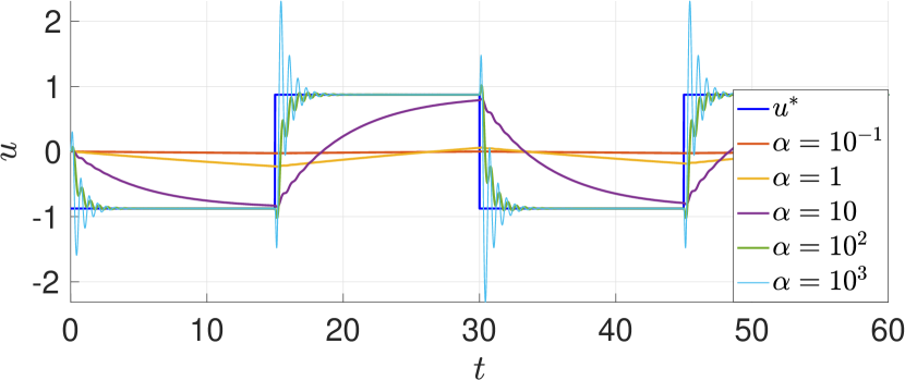
Figure 1: Performance of the OFO controller in (10) for the linear plant in Section V-A and different values of $\alpha$.

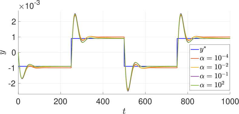
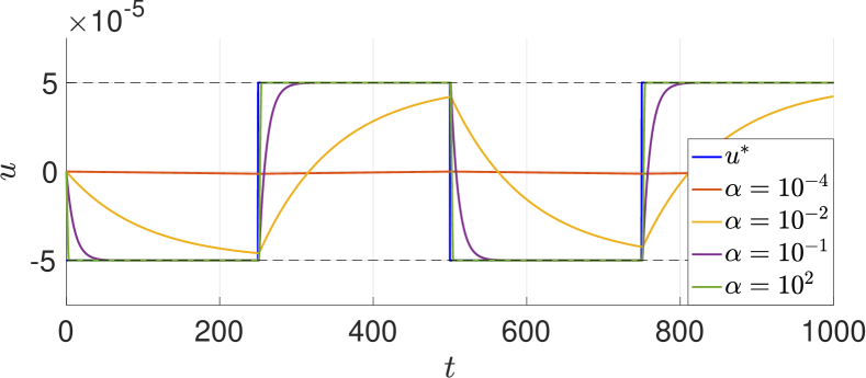
Figure 2: The plant in Section V-B in closed-loop with (19). Input constraints (dotted lines) are always satisfied.

V-B Nonlinear plant with input constrain

We consider the plant $\dot{x}=Ax+B(u+\operatorname{sin}(u))+B_{w}w$, $y=Cx$, where

$$A=\begin{bmatrix}0&-0.1\\ 0.1&-0.1\end{bmatrix},B=\begin{bmatrix}0\\ 0.1\end{bmatrix},B_{w}=\begin{bmatrix}0.1\\ 0.1\end{bmatrix},C=\begin{bmatrix}1&1\end{bmatrix},$$

and $w$ is an unmeasured disturbance. The cost function is given by $\Phi(u,y)=20u^{2}+\sqrt{y^{2}+1}$. The input is constrained as $-5\cdot 10^{-5}\leq u\leq 5\cdot{10^{-5}}$.

Assumption 3(a) holds with $\ell_{f}=2\|B\|$ (by computing $\nabla_{u}f(x,u)$, since $\cos(u)\leq 1$), $\ell_{g}=\|C\|$. The matrix $A$ is Hurwitz, hence the plant has a steady-state map $s(u)=-A^{-1}(Bu+B\operatorname{sin}(u)+B_{w}w)$. We solve the Lyapunov inequality $AP+PA^{\top}+0.045P\prec 0$. Given the solution $P=\left[\begin{smallmatrix}0.66&0.33\\ 0.33&0.66\end{smallmatrix}\right]$ we define the Lyapunov function $W(x,u)=(x-s(u))^{\top}P(x-s(u))$ in Assumption 4 (note that $\nabla_{x}W(x,u)^{\top}f(x,u)=2(x-s(u))^{\top}P(Ax+Bu+B\operatorname{sin}(u)+B_{w}w)=(x-s(u))^{\top}(PA+PA^{\top})(x-s(u))\leq-0.045(x-s(u))^{\top}P(x-s(u))$). Thus, Assumption 4(b) holds with $\mu_{3}=0.45\lambda_{\mathop{\rm min}}(P)$, $d_{3}=\zeta_{3}=\lambda_{\max}(P)$, $c_{3}=\lambda_{\mathop{\rm min}}(P)$. Also, $\|\nabla h(u)\|=\|CA^{-1}B(1+\operatorname{cos}u)\|\leq 2\|CA^{-1}B\|\coloneqq\ell_{h}$ is bounded and $\sqrt{y^{2}+1}$ is $1$-Lipschitz continuous, so Assumption 4(c) holds with $\ell_{\Phi_{y}}=\ell_{h}$. Similarly, $\|\nabla\sqrt{y^{2}+1}\|=\|y/\sqrt{y^{2}+1}\|\leq 1$ and $\nabla h(u)$ is $\ell_{\nabla h}$-Lipschitz continuous, with $\ell_{\nabla h}=\|CA^{-1}B\|$; therefore Assumption 4(d) holds with $\ell_{\Phi_{u}}=\ell_{\nabla h}$. Finally, $\mu_{\Phi}=40$, the bound in (17) is satisfied, and hence the controller (19) guarantees exponential stability of the plant for any value of $\alpha$, by Corollary 3.

We simulate the controller (19) for different values of $\alpha$, with periodic piecewise constant disturbance. For smaller values of $\alpha$, the controller is slower in adapting to changes in the disturbance, and the output slower in reaching the optimal steady state. Interestingly, for larger values of $\alpha$, the OFO scheme in (19) approximately behaves as a bang-bang controller, where the input quickly switches between its lower and upper bounds.

VI Conclusion and research directions

We showed that, under suitable assumptions, online feedback optimization controllers guarantee stability without requiring any timescale separation. Although we framed our results in continuous-time, discrete-time OFO controllers can be studied with analogous assumptions and convergence results. Our analysis can be also extended to tracking the equilibrium trajectory for problems with time-varying disturbances and costs, where our results can be beneficial in achieving better tracking guarantees, by allowing for larger control gains. Future research should focus on implementing more realistic simulation scenarios, to validate the applicability of our results. Further, in this paper we only focused on the analysis of an existing OFO scheme. Developing new control strategies for OFO, specifically designed to avoid the need for timescale separation, and under less restrictive assumptions, is a significant direction for future work.

References

- [1] A. Hauswirth, Z. He, S. Bolognani, G. Hug, and F. Dörfler, “Optimization algorithms as robust feedback controllers,” Annual Reviews in Control, vol. 57, p. 100941, 2024.
- [2] J. W. Simpson-Porco, “On stability of distributed-averaging proportional-integral frequency control in power systems,” IEEE Control Systems Letters, vol. 5, no. 2, pp. 677–682, 2020.
- [3] X. Chen, C. Zhao, and N. Li, “Distributed automatic load frequency control with optimality in power systems,” IEEE Transactions on Control of Network Systems, vol. 8, no. 1, pp. 307–318, 2020.
- [4] Y. Tang, K. Dvijotham, and S. Low, “Real-time optimal power flow,” IEEE Transactions on Smart Grid, vol. 8, no. 6, pp. 2963–2973, 2017.
- [5] E. Dall’Anese, “Optimal power flow pursuit,” in Proceedings of American Control Conference, 2016, pp. 1767–1767.
- [6] G. Belgioioso, D. Liao-McPherson, M. H. de Badyn, S. Bolognani, J. Lygeros, and F. Dörfler, “Sampled-data online feedback equilibrium seeking: Stability and tracking,” in Proceedings of 60th IEEE Conference on Decision and Control, 2021, pp. 2702–2708.
- [7] G. Bianchin, J. Cortés, J. I. Poveda, and E. Dall’Anese, “Time-varying optimization of LTI systems via projected primal-dual gradient flows,” IEEE Transactions on Control of Network Systems, vol. 9, no. 1, pp. 474–486, 2021.
- [8] J. Wang and N. Elia, “A control perspective for centralized and distributed convex optimization,” in 2011 50th IEEE conference on decision and control and European control conference. IEEE, 2011, pp. 3800–3805.
- [9] L. Ortmann, C. Rubin, A. Scozzafava, J. Lehmann, S. Bolognani, and F. Dörfler, “Deployment of an online feedback optimization controller for reactive power flow optimization in a distribution grid,” in 2023 IEEE PES Innovative Smart Grid Technologies Europe (ISGT EUROPE), 2023, pp. 1–6.
- [10] K. B. Ariyur and M. Krstić, Real‐Time Optimization by Extremum‐Seeking Control. Wiley, 2003.
- [11] Z. He, S. Bolognani, J. He, F. Dörfler, and X. Guan, “Model-free nonlinear feedback optimization,” IEEE Transactions on Automatic Control, pp. 1–16, 2023.
- [12] M. Picallo, L. Ortmann, S. Bolognani, and F. Dörfler, “Adaptive real-time grid operation via online feedback optimization with sensitivity estimation,” Electric Power Systems Research, vol. 212, p. 108405, 2022.
- [13] V. Häberle, A. Hauswirth, L. Ortmann, S. Bolognani, and F. Dörfler, “Non-convex feedback optimization with input and output constraints,” IEEE Control Systems Letters, vol. 5, no. 1, pp. 343–348, 2021.
- [14] A. Bernstein, E. Dall’Anese, and A. Simonetto, “Online primal-dual methods with measurement feedback for time-varying convex optimization,” IEEE Transactions on Signal Processing, vol. 67, no. 8, pp. 1978–1991, 2019.
- [15] A. Colot, Y. Chen, B. Cornelusse, J. Cortés, and E. Dall’Anese, “Optimal power flow pursuit via feedback-based safe gradient flow,” 2024. [Online]. Available: https://arxiv.org/abs/2312.12267
- [16] S. Menta, A. Hauswirth, S. Bolognani, G. Hug, and F. Dörfler, “Stability of dynamic feedback optimization with applications to power systems,” in Proceedings of 56th Annual Allerton Conference on Communication, Control, and Computing. IEEE, 2018, pp. 136–143.
- [17] A. Hauswirth, S. Bolognani, G. Hug, and F. Dörfler, “Timescale separation in autonomous optimization,” IEEE Transactions on Automatic Control, vol. 66, no. 2, pp. 611–624, 2021.
- [18] G. Belgioioso, D. Liao-McPherson, M. H. de Badyn, S. Bolognani, R. S. Smith, J. Lygeros, and F. Dörfler, “Online feedback equilibrium seeking,” IEEE Transactions on Automatic Control, pp. 1–16, 2024.
- [19] M. Colombino, E. Dall’Anese, and A. Bernstein, “Online optimization as a feedback controller: Stability and tracking,” IEEE Transactions on Control of Network Systems, vol. 7, pp. 422–432, 3 2020.
- [20] M. Picallo, S. Bolognani, and F. Dörfler, “Sensitivity conditioning: Beyond singular perturbation for control design on multiple time scales,” IEEE Transactions on Automatic Control, vol. 68, no. 4, pp. 2309–2324, 2023.
- [21] D. P. Bertsekas and J. N. Tsitsiklis, Parallel and Distributed Computation: Numerical Methods. Prentice-Hall, USA, 1989. [Online]. Available: http://athenasc.com/pdcbook.html
- [22] T. Hu, L. Ma, and Z. Lin, “Stabilization of switched systems via composite quadratic functions,” IEEE Transactions on Automatic Control, vol. 53, no. 11, pp. 2571–2585, 2008.
- [23] D. T. A. Nguyen, M. Bianchi, F. Dörfler, D. T. Nguyen, and A. Nedić, “Nash equilibrium seeking over digraphs with row-stochastic matrices and network-independent step-sizes,” IEEE Control Systems Letters, vol. 7, pp. 3543–3548, 2023.
- [24] A. Davydov, S. Jafarpour, and F. Bullo, “Non-Euclidean contraction theory for robust nonlinear stability,” IEEE Transactions on Automatic Control, vol. 67, no. 12, pp. 6667–6681, 2022.
- [25] S. Sastry, Nonlinear systems. Springer New York, NY, 1999.