SoftVQ-VAE: Efficient 1-Dimensional Continuous Tokenizer

Abstract

Efficient image tokenization with high compression ratios remains a critical challenge for training generative models. We present SoftVQ-VAE, a continuous image tokenizer that leverages soft categorical posteriors to aggregate multiple codewords into each latent token, substantially increasing the representation capacity of the latent space. When applied to Transformer-based architectures, our approach compresses 256$\times$256 and 512$\times$512 images using as few as 32 or 64 1-dimensional tokens. Not only does SoftVQ-VAE show consistent and high-quality reconstruction, more importantly, it also achieves state-of-the-art and significantly faster image generation results across different denoising-based generative models. Remarkably, SoftVQ-VAE improves inference throughput by up to 18x for generating 256$\times$256 images and 55x for 512$\times$512 images while achieving competitive FID scores of 1.78 and 2.21 for SiT-XL. It also improves the training efficiency of the generative models by reducing the number of training iterations by 2.3x while maintaining comparable performance. With its fully-differentiable design and semantic-rich latent space, our experiment demonstrates that SoftVQ-VAE achieves efficient tokenization without compromising generation quality, paving the way for more efficient generative models. Code and model are released .

Figure 1: ImageNet-1K 256$\times$256 and 512$\times$512 generation results of generative models trained on SoftVQ-VAE with 32 and 64 tokens.

1 Introduction

Denoising-based generative modeling has witnessed remarkable progress with recent advances, such as Diffusion Transformers (DiT) [80], Scalable Interpolant Transformers (SiT) [72], and Masked Auto-Regressive models with diffusion loss (MAR) [60], to name a few. Denosing-based generative modeling not only presents impressive generation results on a wide range of modality, including natural language [32, 122], images [83, 16, 88, 69, 25], videos [42, 8, 6], and audios [81, 24], but also shows potential to unify the understanding and generation capabilities across modalities in multi-modal language models [123, 110, 107, 109].

A core component of denoising-based generative models is the tokenizer [51, 38, 104, 84, 23, 117, 56, 112], which compresses the raw data of each modality into a set of latent tokens in either a discrete or continuous latent space. The compact latent space therefore allows for more efficient and better generative modeling [88]. Among previous efforts, Kullback–Leibler Variational Auto-Encoders (KL-VAE) [51] and Vector Quantized Variational Auto-Encoders (VQ-VAE) [104, 84, 23] stand out as representatives of tokenizers which introduce continuous and discrete latent spaces, respectively. The former constrains the latent space with a Gaussian distribution using re-parametrization [51] trick, and the latter makes its latent space a categorical discrete distribution with a codebook of finite vocabulary which requires straight-through estimation [7].

Although both KL-VAE and VQ-VAE (and their variants) have been predominantly adopted in many generative models [88, 80, 10, 98, 123], they still present two major challenges restricting the efficiency and effectiveness of generative modeling: (1) the difficulty of achieving a higher compression ratio [13] and (2) the worse discriminative representations in their latent space than other self-supervised methods [35, 14, 116, 109]. The efficiency of downstream generative models, particularly Transformer-based architectures [105], is fundamentally constrained by their quadratic complexity to the number of latent tokens. Current image tokenizers [23, 88, 96] typically compress 256$\times$256 images to at least 256 tokens and 512$\times$512 images to at least 1024 tokens, creating a significant computational bottleneck for both training and inference of generative models [80, 72, 60]. Many efforts have been made to reduce the number of latent tokens on the generative model side, such as merging [80, 72, 62], pooling [58, 94, 61], and others [70, 63, 12]. More studies have recently emerged to fundamentally reduce the token number of the tokenizer [30, 115, 62, 11]. For example, TiTok [115] uses 128 tokens, achieving generation results comparable to 256 tokens by adding one extra decoder. DC-AE [11] compresses the initial 1024 tokens of 512$\times$512 with 256 tokens. However, further increasing the compression ratio results in a significant degradation in the quality of reconstruction and therefore the generation [11].

Beyond the compression challenge, the quality of the learned representations of the tokenizer poses another critical limitation. While latent representations are crucial for both understanding [31, 109] and generation tasks [30, 64, 116, 62], current tokenizers usually struggle to capture more discriminative features. Earlier methods attempted to advance the training objectives and recipe to improve the latent space of the tokenizer [23, 19, 34, 124, 14]. Recently, [30, 118, 113, 124, 109, 62, 116] has also explored the representation alignment of latent tokens. However, due to the lossy nature [91, 77] of the smoothness constraints in KL-VAE and the discrete quantization in VQ-VAE [38, 13, 126, 27], current tokenizers usually fall short in learning the semantics of the latent space [109].

To address the aforementioned challenges, we present SoftVQ-VAE, a simple modification to VQ-VAE that converts it from a discrete tokenizer into a continuous one with a high compression ratio and a semantic-rich latent space. Specifically, we propose using a soft categorical posterior in VAE with a learnable codebook. This straightforward modification introduces a crucial capability: instead of the conventional one-to-one mapping between tokens and codewords in VQ-VAE, our approach enables the adaptive aggregation of multiple codewords into each latent token, substantially increasing the representation capacity of the latent space. We apply SoftVQ-VAE to the Transformer auto-encoder architecture [111, 30, 58, 115, 62], and we succeed in using much fewer 1-dimensional latent tokens (i.e., 32 and 64) for both the reconstruction and subsequent generation tasks. Since SoftVQ-VAE is now fully differentiable, it not only simplifies the learning of the codebook, not requiring the codebook loss or commit loss as in VQ-VAE [104, 23], but also enables better representation learning through direct alignment with pre-trained semantic features using a simple cosine similarity objective. Our approach generalizes the K-Means [67] latent space of VQ-VAE to Soft K-Means [22] and further to Gaussian Mixture Models (GMM) [86], while maintaining compatibility with existing VQ-VAE techniques [45, 112, 55, 62]. We comprehensively demonstrate the efficiency and effectiveness of the proposed SoftVQ-VAE in image reconstruction and generation tasks, and show that:

• SoftVQ-VAE presents more consistent, robust, and high-quality reconstruction and generation results with various latent token lengths ranging from 256 to 32.

• SoftVQ-VAE allows diffusion-based DiT [73], flow-based SiT [72], and autoregressive-based MAR [60] to achieve state-of-the-art generation results with only 64 and 32 tokens on both the 256$\times$256, with an FID of 1.78, and 512$\times$512 on ImageNet benchmark, with an FID of 2.21.

• SoftVQ-VAE improves the inference throughput by 18x and 10x with 32 and 64 tokens to generate 256$\times$256 images, and 55x with 64 tokens for generating 512$\times$512 images, with significantly lower GFLOPs for all models.

• SoftVQ-VAE presents a more discriminative latent space through representation alignment. It also facilitates training efficiency by significantly improving training throughput and reduces training iterations by 2.3x.

2 Preliminary

We present an overview of the tokenizers, i.e., KL-VAE [51] and VQ-VAE [104], and denoising-based generative models, i.e., DiT [80], SiT [72], and MAR [60], in this section.

2.1 Image Tokenizer

The architecture of image tokenizer generally resembles auto-encoders, consisting of two main components: an encoder $\mathcal{E}$ and a decoder $\mathcal{D}$, parameterized by $\phi$ and $\theta$, respectively. Given an input image $\mathbf{x}\in\mathbb{R}^{H\times W\times 3}$, the encoder $\mathcal{E}$ maps the high-dimensional $\mathbf{x}$ to a lower-dimensional latent representation $\mathbf{z}=\mathcal{E}(\mathbf{x};\phi)$. The latent representations can have varying shapes depending on the encoder architecture. We generally view the latent representation as a set of latent tokens $\mathbf{z}=[\mathbf{z}^{[0]},\mathbf{z}^{[1]},\dots,\mathbf{z}^{[L]}]\in\mathbb{R}^{L\times D}$, where $L$ is the number of tokens and $D$ is the dimension of the latent representation. For basic auto-encoders (AE), the decoder takes latent tokens as input and reconstructs the original signal $\hat{\mathbf{x}}=\mathcal{D}(\mathbf{z};\theta)$ by minimizing the reconstruction loss with $\mathbf{x}$.

Variational auto-encoders (VAE) [51] extend the basic AE by introducing a probabilistic perspective on the latent space. Specifically, VAE approximates a posterior distribution $p(\mathbf{z}|\mathbf{x})$ with a learned distribution $q_{\phi}(\mathbf{z}|\mathbf{x})$ from the encoder, assuming that $\mathbf{x}$ is generated by the unobserved latent $\mathbf{z}$ with a prior distribution $p(\mathbf{z})$. The decoder instead takes a set of sampled latent tokens $\mathbf{z}\sim q_{\phi}(\mathbf{z}|\mathbf{x})$ from the posterior and aims to learn the marginal likelihood of data in a generative process by optimizing the evidence lower bound (ELBO): $\max_{\phi,\theta}\mathbb{E}_{q_{\phi}(\mathbf{z}|\mathbf{x})}\log p_{\theta}(\mathbf{x}|\mathbf{z})-\mathcal{L}_{\mathrm{kl}}(q_{\phi}(\mathbf{z}|\mathbf{x})|p(\mathbf{z}))$. To make the optimization tractable, assumptions have been made on the prior, leading to different variants of VAE.

KL-VAE [51, 38] parametrizes both the prior and posterior as Gaussians. The prior $p(\mathbf{z})$ is assumed to be the isotropic unit Gaussian $\mathcal{N}(0,1)$. The continuous latent code is parameterized with posterior mean $\boldsymbol{\mu}_{\phi}$ and variance $\boldsymbol{\sigma}^{2}_{\phi}$ predicted by the encoder using the “re-parametrization” trick with a noise variable $\boldsymbol{\varepsilon}$ from standard Gaussian:

While KL-VAE is widely used in diffusion models, it is known to have the “posterior-collapse” issue [13]. In addition, the KL loss weight usually imposes a trade-off between the quality of reconstruction and the smoothness of its latent space [100], preventing high compression ratio and the learning of semantics in the latent space of KL-VAE.

VQ-VAE [104, 23], in contrast, generates latent code in a discrete space by taking the posterior as a $K$-way deterministic categorical distribution against a learnable codebook $\mathcal{C}=[\mathbf{c}^{[0]},\dots,\mathbf{c}^{[K]}]\in\mathbb{R}^{K\times D}$, with $\mathbf{c}$ as the codeword:

Due to the non-differentiable $\operatorname*{arg\,min}$, a “straight-through” trick [7] is adopted to approximate the gradient of the encoder output $\hat{\mathbf{z}}$ by directly copying gradient from the decoder input $\mathbf{z}$. Since the reconstruction objective does not impose direct gradients on the codebook $\mathcal{C}$, VQ-VAE additionally uses a codebook loss as $\|\text{sg}[\hat{\mathbf{z}}]-\mathbf{c}\|_{2}$ to move codewords toward the encoder output, along with a commit loss $\|\hat{\mathbf{z}}-\text{sg}[\mathbf{c}]\|_{2}$ to prevent arbitrary growth of codewords, where $\text{sg}[\cdot]$ denotes stop-gradient. The broken gradient hinders high compression ratio and latent space learning [43, 27].

2.2 Denoising-based Generative Models

Denoising-based generative models synthesize images by progressively transforming Gaussian noise $\boldsymbol{\varepsilon}\sim\mathcal{N}(0,\mathbf{I})$ into tokenizer latent codes $\mathbf{z}$ through a forward process [92, 41]:

$$\mathbf{z}_{t}=\alpha_{t}\mathbf{z}+\sigma_{t}\varepsilon,$$ (3)

where $\alpha_{t}$ and $\sigma_{t}$ are a decreasing and increasing function of $t$, and $t\in[0,T]$ [50]. In this paper, we adopt three approaches to implementing this denoising process as follows.

DiT [80] is a diffusion-based model with a transformer architecture. It formulates the process through a forward-time stochastic differential equation (SDE), where $\mathbf{z}_{t}$ converges to $\mathcal{N}(0,\mathbf{I})$ as $t\rightarrow T$. Generation occurs via a reverse-time SDE [2], with the model trained to predict noise $\boldsymbol{\varepsilon}$ at randomly sampled timesteps. Due to the long token length of the tokenizer [96] used in DiT, it has several variants to merge tokens at the input of the transformer backbone.

SiT [72] instead uses stochastic interpolants [1] and performs denoising via probability flow ordinary differential equation (PF ODE). The model learns the ODE’s velocity field [65] by minimizing mean-squared-error (MSE) with the interpolated noise. This velocity field defines a score function for sample generation, analogous to DiT’s reverse-time SDE.

MAR [60] combines diffusion with autoregressive generation. Unlike DiT and SiT’s parallel denoising of all latent tokens, MAR adopts an encoder-decoder transformer architecture [35] that progressively denoises tokens in a “next-set” autoregressive manner [99], starting from masked tokens, similar to MaskGIT [10] and MAGE [59].

3 Method

In this section, we present SoftVQ-VAE, a novel 1D continuous tokenizer with a high compression ratio and a semantic-rich latent space. We first introduce the architecture and the formulation of SoftVQ-VAE. Then, we show that SoftVQ-VAE can learn semantics easily by aligning its latent tokens with pre-trained features via its fully-differentiable property.

3.1 Architecture

Figure 2: Illustration of SoftVQ-VAE. Left: Transformer encoder-decoder architecture with image tokens, arbitrary length of latent tokens, and mask tokens. Right top: fully-differentiable SoftVQ illustration. Right bottom: latent space representation alignment.

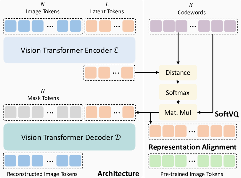
We leverage Vision Transformer (ViT) [21, 111] as the architecture for the encoder $\mathcal{E}$ and decoder $\mathcal{D}$ of SoftVQ-VAE. Similarly to Yu et al. [115], instead of using the image features as latent, we initialize a set of extra 1D learnable tokens and use these tokens for reconstruction and subsequent generation. With the self-attention mechanism, it allows the learnable tokens to adaptively aggregate different image tokens to obtain the latent tokens of SoftVQ, detailed in Sec. 3.2. Specifically, for the encoder transformer with a patch size of $P$, an image $\mathbf{x}\in\mathbb{R}^{H\times W\times 3}$ is patchified into a sequence of image tokens $\mathbf{x}_{p}\in\mathbb{R}^{N\times D}$, where $N=\ HW/P^{2}$ and $D$ represent the token dimension size. We then concatenate a set of learnable tokens $\mathbf{z}_{l}\in\mathbb{R}^{L\times D}$ of length $L$ along with the image tokens as the input to the encoder, and retain only the output corresponding to the learnable latent tokens as the output of our encoder: $\hat{\mathbf{z}}=\mathcal{E}([\mathbf{x}_{p};\mathbf{z}_{l}];\phi)$.

For the decoder, we reconstruct images from a sequence of learnable mask tokens $\mathbf{m}\in\mathbb{R}^{N\times D}$ [5, 35], concatenated with latent tokens: $\hat{\mathbf{x}}=\mathcal{D}([\mathbf{m};\mathbf{z}];\theta)$. We use a linear layer at the end of the decoder to regress the pixel values from the mask tokens. For the image tokens at the encoder input and mask tokens at the decoder input, we apply 2D absolute position embeddings and 1D absolute position embedding for the latent tokens. Adopting more advanced position embedding techniques, such as RoPE [97, 36], may lead to better results and is left for future work. This design allows SoftVQ-VAE to use latent codes of arbitrary length, each adaptively associated with image tokens, for reconstruction and subsequent generative modeling, and model images of various resolutions using the same length of latent codes. An overview of the model architecture is shown in Fig. 2.

3.2 SoftVQ-VAE

As discussed above, the high compression ratio of both KL-VAE and VQ-VAE usually results in a significant degradation of quality in reconstruction and latent space. To overcome these limitations, we propose SoftVQ-VAE, a simple modification to VQ-VAE, which maintains the advantages of learning codewords to capture the data distribution while bridging it with more representation capacity as a continuous tokenizer. The core idea of SoftVQ-VAE is to allow each latent code to adaptively aggregate multiple codewords from the learnable codebook. Consequently, it imposes a soft categorical distribution on the posterior from the encoder:

where $\tau$ is the temperature parameter controlling the sharpness of the softmax probability and is set to $0.07$ by ablation. The derivation of $\mathcal{L}_{kl}$ is shown in Sec. B.1.

Despite this simple modification, SoftVQ-VAE can significantly reduce the latent token length while maintaining a high quality of the reconstruction and latent space. More importantly, with a soft categorical distribution, SoftVQ-VAE is fully-differentiable, and thus the encoder and codebook can be optimized directly from the reconstruction loss (and other losses). It also allows for easier regularization of various forms on the latent space that drastically improves its quality, and less hyper-parameter tuning without codebook and commit loss [43] in the reduced training objectives.

Interpretation. The posterior and latent space of VQ-VAE can be interpreted with K-Means [67]. Hence, SoftVQ-VAE can be viewed as soft K-Means [22], with codewords as learnable prototypes in the latent space. This latent space can easily be extended to Gaussian Mixture Models (GMM) [86], which we refer to as GMMVQ-VAE. Instead of using fixed temperature, GMMVQ-VAE predicts data-dependent weights for the codeword prototypes, i.e., Gaussian means, to compute the soft categorical posterior: $q_{\phi}(\mathbf{z}|\mathbf{x})=\operatorname*{Softmax}(-\omega(\hat{\mathbf{z}})\|\hat{\mathbf{z}}-\mathcal{C}\|_{2})$. Although prior work has explored GMM-based VAEs [17, 47], our GMMVQ-VAE differs by learning discrete prototypes rather than continuous latent variables. While providing the additional benefit of interpretable Gaussian components in the latent space, GMMVQ achieves reconstruction quality and downstream generation performance similar to SoftVQ in our experiments, and thus we mainly adopt the simpler SoftVQ throughout this paper. More details are in Sec. B.2.

3.3 Representation Alignment of Latent Space

While the reconstruction quality of tokenizer is important, learning a high-quality latent space is more crucial for downstream denoising-based generative modeling [116]. Several recent approaches have explored aligning the latent code with pre-trained features through a contrastive loss [30, 109, 62] and initializing the codebook with pre-trained features [124]. However, imposing effective regularization on the latent remains a challenge due to the discrete quantization of VQ-VAE and the Gaussian constraints in KL-VAE.

Thanks to the fully-differentiable property of SoftVQ-VAE, we can now directly impose regularization on the latent space. Inspired by the recent work of REPA [116], we propose aligning the representations of latent codes with pre-trained vision encoders to facilitate learning the latent space. Compared to REPA, which aligns the representation at intermediate layers of downstream generative models, our method of feature alignment in the tokenizer’s latent space is equivalent to performing REPA at the input space of generative models. Specifically, to align the latent code with the image tokens from a pre-trained vision encoder, we replicate each latent token by $N/L$ times:

$$\mathbf{z}_{r}=[\underbrace{\mathbf{z}^{[0]},\ldots,\mathbf{z}^{[0]}}_{N/L\text{ times}},\underbrace{\mathbf{z}^{[1]},\ldots,\mathbf{z}^{[1]}}_{N/L\text{ times}},\ldots,\underbrace{\mathbf{z}^{[L]},\ldots,\mathbf{z}^{[L]}}_{N/L\text{ times}}],$$ (5)

and encourage the token-wise similarity with image tokens. We employ a projector multilayer perceptron (MLP) on top of the latent tokens to match the pre-trained feature $\mathbf{y}_{*}$:

$$\mathcal{L}_{\mathrm{align}}=\frac{1}{N}\sum_{n=1}^{N}\operatorname{sim}\left(\mathbf{y}_{*}^{[n]},\text{MLP}\left(\mathbf{z}_{r}^{([n]}\right)\right).$$ (6)

This alignment ensures the latent space of SoftVQ-VAE captures semantically discriminative features that are beneficial for training the downstream generative models, even if it does not directly translate into improved reconstruction performance from the tokenizer. However, as we will show in Sec. 4.4, the generation quality of trained generative models often depends more on the semantic structure of the latent space than on the tokenizer’s reconstruction capabilities.

3.4 Final Training Objective

The training objective of SoftVQ-VAE combines the reconstruction loss, perceptual loss [54, 46, 20, 120] and adversarial loss [33, 44] as in VQ [23], and representation alignment:

$$\mathcal{L}=\mathcal{L}_{\textrm{recon}}+\lambda_{1}\mathcal{L}_{\textrm{percep}}+\lambda_{2}\mathcal{L}_{\textrm{adv}}+\lambda_{3}\mathcal{L}_{\textrm{align}}+\lambda_{4}\mathcal{L}_{\textrm{KL}},$$ (7)

where $\lambda_{1}$, $\lambda_{2}$, $\lambda_{3}$, and $\lambda_{4}$ are hyper-parameters. Neither codebook nor commit loss as in VQ is needed. The perceptual loss $\mathcal{L}_{\textrm{percep}}$ helps capture high-level perceptual features, $\mathcal{L}_{\textrm{adv}}$ encourages the decoder to generate realistic images by removing the artifacts from the reconstruction loss only, $\mathcal{L}_{\textrm{align}}$ guides the latent space to align with pre-trained features, and $\mathcal{L}_{\textrm{kl}}$ as the KL divergence term in the ELBO.

4 Experiments

In this section, we validate the efficiency and effectiveness of SoftVQ-VAE with extensive experiments.

Table 1: System-level comparison on ImageNet 256$\times$256 conditional generation. We compare with both diffusion-based models and auto-regressive models with different types of tokenizers. Grey denotes SoftVQ. ^† indicates results with DPM-Solver and 50 steps.

Gen. Model	Tok. Model	# Tokens $\downarrow$	Tok. rFID $\downarrow$	Gflops $\downarrow$	Throughput (imgs/sec) $\uparrow$	w/o CFG		w/ CFG
						gFID $\downarrow$	IS $\uparrow$	gFID $\downarrow$	IS $\uparrow$
Auto-regressive Models
Taming-Trans. [23]	VQ	256	7.94	-	-	5.20	290.3	-	-
RQ-Trans. [55]	RQ	256	3.20	908.91	7.85	3.80	323.7	-	-
MaskGIT [10]	VQ	256	2.28	-	-	6.18	182.1	-	-
MAGE [59]	VQ	256	-	-	-	6.93	195.8	-	-
LlamaGen-3B [98]	VQ	256	2.19	781.56	2.90	-	-	3.06	279.7
TiTok-S-128 [115]	VQ	128	1.61	33.03	6.50	-	-	1.97	281.8
MAR-H [60]	KL	256	1.22	145.08	0.12	2.35	227.8	1.55	303.7
	SoftVQ-L	32	0.61	67.93	2.08	3.83	211.2	2.54	273.6
MAR-H	SoftVQ-BL	64	0.65	86.55	0.89	2.81	218.3	1.93	289.4
Diffusion-based Models
LDM-4 [88]	KL	4096	0.27	157.92	0.37	10.56	103.5	3.60	247.7
U-ViT-H/2† [4]	KL	1024	0.62	128.89	0.98	-	-	2.29	263.9
MDTv2-XL/2 [29]				125.43	0.59	5.06	155.6	1.58	314.7
DiT-XL/2 [80]				80.73	0.51	9.62	121.5	2.27	278.2
SiT-XL/2 [72]				81.92	0.54	8.30	131.7	2.06	270.3
+ REPA [116]						5.90	157.8	1.42	305.7
	SoftVQ-B		0.89		8.94	9.83	113.8	3.91	264.2
	SoftVQ-BL		0.68		8.81	9.22	115.8	3.78	266.7
DiT-XL	SoftVQ-L	32	0.74	14.52	8.74	9.07	117.2	3.69	270.4
	SoftVQ-B		0.88		4.70	6.62	129.2	3.29	262.5
	SoftVQ-BL		0.65		4.59	6.53	131.9	3.11	268.3
DiT-XL	SoftVQ-L	64	0.61	28.81	4.51	5.83	141.3	2.93	268.5
	SoftVQ-B		0.89		10.28	7.99	129.3	2.51	301.3
	SoftVQ-BL		0.68		10.12	7.67	133.9	2.44	308.8
SiT-XL	SoftVQ-L	32	0.74	14.73	10.11	7.59	137.4	2.44	310.6
	SoftVQ-B		0.88		5.51	5.98	138.0	1.78	279.0
	SoftVQ-BL		0.65		5.42	5.80	143.5	1.88	287.9
SiT-XL	SoftVQ-L	64	0.61	29.23	5.39	5.35	151.2	1.86	293.6

4.1 Experiments Setup

Implementation Details of SoftVQ-VAE. We use the LlamaGen codebase [98] to build our SoftVQ-VAE. We instantiate 4 configurations: SoftVQ-S, SoftVQ-B, SoftVQ-BL, SoftVQ-L, with a total of 45M, 173M, 391M, and 608M parameters, respectively. Each configuration has variants of latent codes $L=64$ and $L=32$. For the representation alignment, we choose DINOv2 [79] for the pre-trained features, similarly as Yu et al. [116] and Li et al. [62]. To learn a better semantic latent space, we initialize our encoder from the pre-trained DINOv2 weights. Alignment with other pre-trained features is explored in Sec. 4.4. We train the tokenizers on ImageNet [15] of resolution 256$\times$256 and 512$\times$512 for 250K iterations. Similarly to Tian et al. [99] and Li et al. [62], we found that the discriminator is very important for training tokenizer, and we adopted the same frozen DINO-S [9, 79] discriminator with a similar architecture to StyleGAN [48, 49]. In addition, we use DiffAug [121], consistency regularization [119], and LeCAM regularization [101] for discriminator training as in [99]. For the training objective, we set $\lambda_{1}=1.0$, $\lambda_{1}=0.2$, $\lambda_{3}=0.1$, and $\lambda_{4}=0.01$, following previous common practice. More training details are shown in Sec. C.1.

Implementation Details of Generative Modeling. We select DiT [80], SiT [57], and MAR [60] for downstream denoising-based image generation tasks. For DiT and SiT, we set the patch size of DiT and SiT to 1 and use a 1D absolution position embedding. In our main experiments, we train DiT-XL and SiT-XL of 675M parameters for 3M steps, compared to 4M steps in REPA [116] and 7M steps vanilla version [80, 72]. We strictly follow their original training setup for other settings. For MAR-H, we train for 500 epochs and set the maximum learning rate to 2$e$-4 since a higher learning rate leads to NAN issues. For other experiments, we simply train SiT-L of 458M parameters for 400K steps. More experimental details are provided in Sec. C.2.

Evaluation. We use reconstruction Frechet Inception Distance (rFID) [37] on ImageNet validation set to evaluate the tokenizer. To evaluate the performance of generation tasks, we report generation FID (gFID), Inception Score (IS) [90], Precision and Recall [52] (in Sec. D.4), with and without classifier-free guidance (CFG) [40]. We measure the efficiency of the generative models by GLOPs of the model’s forward pass on the latent codes of tokenizers, and training and inference throughput for the models using floating point 32 and a batch size of $64$ on a single AMD MI250.

4.2 Main Results

We present the main reconstruction and generation results on the ImageNet benchmark of resolution 256$\times$256 and 512$\times$512 in Tab. 1 and Tab. 2, respectively. We show that SoftVQ-VAE achieves reconstruction and generation performance (with generative models) comparable to leading systems with 32 and 64 tokens, while presenting a significant improvement in both training and inference efficiency.

Consistent high-quality reconstruction. SoftVQ variants achieve remarkable reconstruction quality with a high compression ratio. With only 32 and 64 tokens, our models maintain consistent rFID scores, i.e., 0.61-0.89 on the 256$\times$256 and 0.64-0.71 on 512$\times$512 benchmark, substantially outperforming VQ tokenizers with 256 tokens used in autoregressive models such as MaskGIT [10] and TiTok [115]. Our results are also comparable to KL tokenizers used in previous denoising-based models, using 32x fewer tokens. More discussion of different tokenizers is given in Sec. 4.3.

Table 2: System-level comparison on ImageNet 512$\times$512 conditional generation. We compare with both diffusion-based models and auto-regressive models with different types of tokenizers. Grey denotes SoftVQ. ^† indicates results with DPM-Solver and 50 steps.

Gen. Model	Tok. Model	# Tokens $\downarrow$	Tok. rFID $\downarrow$	Gflops $\downarrow$	Throughput (imgs/sec) $\uparrow$	w/o CFG		w/ CFG
						gFID $\downarrow$	IS $\uparrow$	gFID $\downarrow$	IS $\uparrow$
Generative Adversarial Models
BigGAN [10]	-	-	-	-	-	-	-	8.43	177.9
StyleGAN-XL [48]	-	-	-	-	-	-	-	2.41	267.7
Auto-regressive Models
MaskGIT [10]	VQ	1024	1.97	-	-	7.32	156.0	-	-
TiTok-B [115]	VQ	128	1.52	-	-	-	-	2.13	261.2
MAR-H	SoftVQ-BL	64	0.71	86.55	1.50	8.21	152.9	3.42	261.8
Diffusion-based Models
ADM [16]	-	-	-	-	-	23.24	58.06	3.85	221.7
U-ViT-H/4† [4]	KL	4096	0.62	128.92	0.58	-	-	4.05	263.8
DiT-XL/2 [80]				373.34	0.10	9.62	121.5	3.04	240.8
SiT-XL/2 [72]				373.32	0.10	-	-	2.62	252.2
DiT-XL [11]	AE	256	0.22	80.75	1.02	9.56	-	2.84	-
UViT-H† [11]				128.90	6.14	9.83	-	2.53	-
UViT-H† [11]	AE	64	0.22	32.99	15.23	12.26	-	2.66	-
UViT-2B† [11]				104.18	9.44	6.50	-	2.25	-
SiT-XL	SoftVQ-BL	64	0.71	29.23	5.38	7.96	133.9	2.21	290.5

Generation performance comparable to SOTA. Notably, with only 32 tokens, the generation performance of DiT-XL and SiT-XL trained on all variants of the proposed SoftVQ significantly outperforms DiT-XL/2 and SiT-XL/2 with KL tokenizers of 1024 tokens, without using CFG. DiT-XL with SoftVQ-L of 32 tokens presents a 0.62 improvement on FID and SiT-XL with SoftVQ-L of 32 tokens shows a 0.71 improvement on FID, without using CFG. The improvement is further strengthened with 64 tokens. SiT-XL with SoftVQ-L of 64 tokens outperforms SiT-XL/2 with REPA [116], without using CFG. Applying CFG, SiT-XL with SoftVQ of 64 tokens achieves a performance comparable to the leading systems with the best FID as 1.78 on 256 and 2.21 on 512 benchmark. Using MAR-H [60], SoftVQ-BL and SoftVQ-L with 64 and 32 tokens present slightly worse results, compared to the KL tokenizer of 256 tokens, possibly due to the lowered learning rate. MAR-H and SiT-XL results on 512 benchmark with 32 tokens are included in Sec. D.2.

Efficiency. The system-level comparison reveals SoftVQ’s exceptional efficiency across multiple metrics. When integrated with MAR-H at 256$\times$256 resolution, SoftVQ reduces GFLOPs by  40% compared to standard KL tokenizer, i.e., 86.55 vs 145.08 GFLOPs with 64 tokens and further reducing to 67.93 GFLOPs with 32 tokens. The efficiency gains are even more pronounced in diffusion-based models, especially with higher resolutions. SoftVQ enables DiT-XL and SiT-XL to achieve significantly lower computational costs i.e., 28.81 and 29.23 GFLOPs, respectively with 64 tokens, compared to their KL counterparts (80.73 GFLOPs with 1024 tokens). Importantly, these efficiency improvements come without compromising generation quality. SiT-XL trained on SoftVQ-BL with 64 tokens presents  55x throughput than the KL counterpart, while showing competitive IS and FID scores in all configurations. The improved GFLOPs also lead to a more efficient training. Not only do we require fewer training iterations to achieve a comparable performance to leading systems, i.e., 2.5M vs 7M steps of SiT-XL and DiT-XL, the high compression ratio of SoftVQ also improves the training throughput, reducing the time to train SiT-XL for 400K steps from 72 to 20 hours on 8 MI250.

4.3 Comparison of Tokenizers

We compare the proposed SoftVQ-VAE with the concurrent efficient image tokenizers, i.e., TiTok [115] and DC-AE [11]. To show the superiority of SoftVQ-VAE in achieving a high compression ratio, we additionally train VQ-VAE and AE using the small (S) configuration and the same training recipe of SoftVQ. To validate the generation performance, we train a SiT-L for 400K steps and report gFID and IS on 256 ImageNet without using CFG, as shown in Tab. 3.

Scalable performance. With a much smaller model size, i.e., 46M vs 390M, SoftVQ-S significantly outperforms both TiTok variants at 64 tokens, achieving better reconstruction quality with an rFID of 1.03 compared to 1.25, and better generation performance with a gFID of 11.24 and IS of 89.4 compared to the best TiTok gFID of 19.23 and IS of 61.8. Noteworthy is that the generation results SiT-L trained on SoftVQ with 32 tokens outperform those trained on KL tokenizer with 1024 tokens [72] by a large margin, i.e., 5.9 in gFID. Compared to DC-AE, SoftVQ-S demonstrates competitive scalability across token counts while maintaining significant generation quality even with fewer parameters.

Table 3: Comparison of tokenizers on class-conditional 256$\times$256 ImageNet. We report rFID, and gFID and IS of SiT-L without CFG.

Tokenizer	# Params	# Tokens	Token Dim.	rFID $\downarrow$	SiT-L
					gFID $\downarrow$	IS $\uparrow$
KL [96]	676M	1024	4	0.62	18.79	72.0
TiTok-BL-KL [115]	389M	64	16	1.25	23.35	54.7
TiTok-BL-VQ [115]	390M	64	16	2.06	19.23	61.8
DC-AE-f32 [11]	323M	64	32	0.69	15.36	76.1
DC-AE-f54 [11]	677M	16	128	0.81	24.66	49.1
VQ-S	46M	256	8	1.45	19.02	58.6
		128	16	2.61	18.51	62.4
		64	32	4.04	20.07	54.5
		32	64	10.97	21.57	47.6
AE-S	46M	256	8	1.15	22.11	58.3
		128	16	1.33	22.31	58.5
		64	32	1.64	25.53	54.3
		32	64	2.01	28.18	45.5
SoftVQ-S	46M	256	8	0.80	9.21	93.6
		128	16	0.92	10.12	85.8
		64	32	1.03	11.24	89.4
		32	64	1.24	12.89	79.5

Less Lossy Property. SoftVQ-S exhibits remarkably consistent performance across different compression ratios. When reducing tokens from 256 to 32, SoftVQ-S maintains a minimal degradation in rFID from 0.80 to 1.24, significantly outperforming both VQ-S, from 1.45 to 10.97, and AE-S, from 1.15 to 2.01. The benefits of the fully-differentiable property of SoftVQ along with representation alignment are particularly evident in generation quality, where SoftVQ-S achieves substantially better gFID of 9.21-12.89, and IS scores of 79.5-93.6, compared to baselines, showing its robustness in preserving information at high compression ratios and a better latent space for generative models to be trained on.

4.4 Discussions on the Latent Space

We perform more analysis on the latent of SoftVQ here.

Alignment with different initialization and target models. As shown in Tab. 4, our results demonstrate the effectiveness of alignment across various pre-trained models. The encoder initialization and alignment with DINOv2-B [79] achieve superior performance with rFID 0.88 and IS 103.4, compared to using either component alone. Further improvements are observed with CLIP-B [82] and EVA-02-B [26] on reconstruction. We reveal that a better rFID does not necessarily translate to a better gFID. Instead, the latent space quality, reflected by linear probing accuracy, is more closely related to the performance of the generative models.

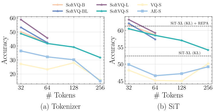
Linear probing of tokenizer and generative model. Linear probing results in Fig. 3 (details in Sec. C.3) reveal SoftVQ’s superior representation quality at both tokenizer and generative model. At the tokenizer level, the linear probing accuracy of SoftVQ variants (B, BL, L) consistently outperforms VQ-S and AE-S across all token counts, with the gaps widening at lower token counts, similarly observed by Yu et al. [115]. This advantage transfers to the generative model with the best linear probing accuracy on the intermediate features of SiT trained with SoftVQ.

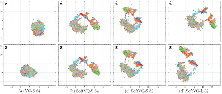
Latent space visualization. UMAP visualizations on the latent space in Fig. 4 demonstrate SoftVQ’s ability to maintain structured and discriminative latent representations with minimal variance between encoder output ($\hat{\mathbf{z}}$) and decoder input ($\mathbf{z}$). Comparing Fig. 4 (d) and (c), we also observe the larger encoder can learn a more discriminative latent space, showing the superiority of SoftVQ’s representation learning.

4.5 Ablation Studies

We present a series of ablation studies in Sec. D.1, including SoftVQ variants with product quantization (PQ) [45], residual quantization (RQ) [55], and GMMVQ, codebook size, latent space size, and the temperature of SoftVQ. The results show the compatibility of SoftVQ with PQ and RQ, with slightly improved performance. GMMVQ presents results comparable to SoftVQ. Moreover, SoftVQ shows robustness to other parameters, such as codebook size and softmax temperature. We found that while increasing the dimension of the latent space can result in a significant improvement in reconstruction, it leads to deterioration in generation performance, possibly due to the learning difficulty of generative models with larger dimensions [92].

Table 4: Representation alignment with different encoder initialization and the target alignment models using SoftVQ-B 64 tokens.

Enc. Init.	Align. Target	rFID $\downarrow$	L.P. $\uparrow$	SiT-L
				gFID $\downarrow$	IS $\uparrow$
-	-	0.98	5.42	20.33	89.4
-	DINOv2-B [79]	0.93	41.08	10.96	101.9
DINOv2-B [79]	-	0.73	11.87	17.20	91.5
DINOv2-B [79]	DINOv2-B [79]	0.88	42.42	10.13	103.4
CLIP-B [82]	CLIP-B [82]	0.75	47.12	9.89	109.3
EVA-02-B [26]	EVA-02-B [26]	0.81	44.23	10.34	112.7

5 Related Work

Image tokenization has emerged as a fundamental technique to bridge various vision tasks. Traditional approaches using autoencoders [39, 106] laid the groundwork by compressing images into latent representations. This field subsequently diverged into two main branches: generation-focused and understanding-focused approaches. Generation-oriented methods, such as VAE [104, 84] and VQ-GAN [23, 85], emphasized learning latent spaces for detail-preserving compression. These were further refined through variants [55, 112, 73, 124] that enhanced generation quality. Parallel developments in understanding-focused approaches leveraged Large Language Models (LLMs) [105] to create semantic representations for tasks like classification [21] and detection [125]. Recent work [115, 62] has demonstrated the potential of unifying these approaches, with subsequent research [109, 34] exploring the convergence of generation and understanding capabilities using a single tokenizer.

Image generation have two popular paradigms: autoregressive and diffusion. Autoregressive models start from CNN-based architectures [103] and evolve to the transformer-based architectures [105, 114, 55, 66, 98] to enhance scalability. Latest works in visual autoregressive modeling, including VAR [99], MAR [60], and ImageFolder [62], have further enhanced generation efficiency. Diffusion models have transformed image generation since their introduction by Sohl-Dickstein et al. [93]. Key advancements by Nichol et al. [75], Dhariwal et al. [16], and Song et al. [95] have significantly improved model performance. A paradigm shift occurred with the adoption of latent space diffusion [102, 88], leveraging pre-trained image encoders as priors [104, 23] to enhance generation efficiency. Architectural innovations, particularly the integration of transformers [80], have further expanded the capabilities of these models. These advances have spawned numerous influential systems, from text-guided generation [76, 18] to high-fidelity synthesis [28, 89]. Commercial successes [83, 87, 74, 78] have also demonstrated the practical impact of diffusion models.

Figure 3: Linear probing accuracy of ImageNet-1K val. set on (a) latent tokens of tokenizer and (b) intermediate features (layer 20) of SiT (L for small and XL for others) trained on latents of tokenizer.

Figure 4: Visualization of $\hat{\mathbf{z}}$ (top), i.e., encoder output, and $\mathbf{z}$ (bottom), i.e., decoder input, of (a) VQ-S 64; (b) SoftVQ-S 64; (c) SoftVQ-S 32; (d) SoftVQ-L 32, trained with latent space alignment.

6 Conclusion

We presented SoftVQ-VAE, a continuous image tokenizer leveraging soft categorical posteriors to aggregate multiple codewords into each latent token. Our approach compresses images to just 32 or 64 tokens while maintaining high reconstruction quality and enabling state-of-the-art generation results with DiT, SiT, and MAR. The substantial improvements in both inference throughput (up to 55x with 64 tokens) and training efficiency, combined with the fully-differentiable design’s ability to learn semantic-rich representations, demonstrate SoftVQ-VAE’s potential as a foundation for efficient generative and vision-language models.

Supplementary Material

Appendix A Posterior of KL-VAE and VQ-VAE

In this section, we provide the detailed derivation of the KL-divergence of KL-VAE and VQ-VAE used in Eq. 1 and Eq. 2, respectively.

KL-VAE has the KL divergence of the posterior with a Gaussian prior:

$$\mathcal{L}_{\mathrm{kl}}\left(q_{\phi}(\mathbf{z})\|p(\mathbf{z})\right).$$ (8)

$$=\int q_{\phi}(\mathbf{z})\left(\log q_{\phi}(\mathbf{z})-\log p(\mathbf{z})\right)d\mathbf{z}$$

$$=\frac{1}{2}\sum_{j=1}^{D}\left(1+\log\left(\left(\sigma_{j}\right)^{2}\right)-\left(\mu_{j}\right)^{2}-\left(\sigma_{j}\right)^{2}\right),$$

where $D$ is the latent space dimension.

VQ-VAE assumes a uniform prior over the total $K$ codewords in the learnable codebook for the deterministic posterior, thus present a KL divergence as follows:

$$\mathcal{L}_{\mathrm{kl}}\left(q_{\phi}(\mathbf{z})\|p(\mathbf{z})\right).$$ (9)

$$=\int q_{\phi}(\mathbf{z})\left(\log q_{\phi}(\mathbf{z})-\log p(\mathbf{z})\right)d\mathbf{z}$$

$$=-(-\log K)$$

$$=\log K$$

Appendix B Additional Details of SoftVQ-VAE and its Variants

In this section, we present more details on the posterior of SoftVQ-VAE, its variant GMMVQ-VAE with the latent space as a GMM model, and the compatibility of SoftVQ-VAE with improvement techniques of VQVAE.

B.1 Posterior of SoftVQ-VAE

In SoftVQ, we similarly assume that the prior is a uniform distribution over the $K$ learnable codewords as in VQ, except for we have the posterior as the softmax probability:

$$\mathcal{L}_{\mathrm{kl}}\left(q_{\phi}(\mathbf{z})\|p(\mathbf{z})\right).$$ (10)

$$=\int q_{\phi}(\mathbf{z})\left(\log q_{\phi}(\mathbf{z})-\log p(\mathbf{z})\right)d\mathbf{z}$$

$$=H(q_{\phi}(\mathbf{z}))-H(q_{\phi}(\mathbf{z}),p(\mathbf{z})),$$

where $H(q_{\phi}(\mathbf{z})$ is the entropy for $H(q_{\phi}(\mathbf{z}),p(\mathbf{z}))$ is the cross-entropy between $q_{\phi}(\mathbf{z})$ and the uniform prior $p(\mathbf{z})\sim\mathcal{U}(0,K)$. In practice, $H(\mathbb{E}_{\mathbf{x}\sim p(\mathbf{x})}[q_{\phi}(\mathbf{z})],p(\mathbf{z}))$ we compute the $\mathbb{E}_{\mathbf{x}\sim p(\mathbf{x})}[q_{\phi}(\mathbf{z})]$ instead, where $\mathbb{E}_{\mathbf{x}\sim p(\mathbf{x})}[q_{\phi}(\mathbf{z})]$ is computed on the averaged batch data during training.

B.2 GMMVQ-VAE

As discussed in the main paper, the latent space of SoftVQ can be interpreted as soft K-Means, and it can be further extended to a latent space of Gaussian Mixture Model. We present more details of this extension here.

In GMMVQ-VAE, the encoder predicts two things: the embedding $\hat{\mathbf{z}}$ and the weights of the Gaussian component $\omega(\hat{\mathbf{z}})$. We can then formulate the posterior as:

$$\begin{split}&\textit{posterior: }q_{\phi}(\mathbf{z}|\mathbf{x})=\operatorname*{Softmax}\left(-\omega(\hat{\mathbf{z}})\|\hat{\mathbf{z}}-\mathcal{C}\|_{2}\right)\\ &\textit{latent: }\mathbf{z}=q_{\phi}(\mathbf{z}|\mathbf{x})\mathcal{C}\\ &\textit{kl: }\mathcal{L}_{\mathrm{kl}}=H(q_{\phi}(\mathbf{z}|\mathbf{x}))-H\left(\mathbb{E}_{\mathbf{x}\sim p(\mathbf{x})}q_{\phi}(\mathbf{z}|\mathbf{x})\right).\\ \end{split}$$ (11)

The difference between SoftVQ and GMMVQ in our formulation is the way in computing the posterior, i.e., using fixed temperature parameter versus learning the data-dependent temperature parameters by the encoder. Note that we still maintain the codebook and its codewords entries directly for the decoder input. It is possible to make the latent space formally a GMM, by treating the codewords as Gaussian means, and formulating the decoder input with the re-parametrization trick. However, we find that this formulation with re-parametrization will hinder the learning of the latent space. Thus, we adopted the simpler design to use the codebook directly for reconstruction, assuming fixed variance in the Gaussian components of GMM.

B.3 Compatibility of SoftVQ-VAE

Figure 5: Illustration of product quantization (left) and residual quantization (right) with SoftVQ.

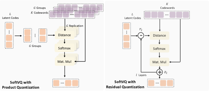
Since SoftVQ-VAE maintains the learnable codebook, previous techniques to improve VQ-VAE are also compatible with it. Here, we follow ImageFolder [62] to show the combination of SoftVQ with product quantization [45] and residual quantization [55], as illustrated in Fig. 5.

Product Quantization (PQ) [45] divides the latent codes into $G$ groups, with each group having its own codebook:

$$\begin{split}\mathbf{z}&=[\mathbf{z}^{(1)},\mathbf{z}^{(2)},...,\mathbf{z}^{(G)}]\\ \quad q_{\phi}(\mathbf{z}^{(g)}|\mathbf{x})&=\operatorname*{Softmax}(-\|\hat{\mathbf{z}}^{(g)}-\mathcal{C}^{(g)}\|_{2}/\tau).\end{split}$$ (12)

PQ can effectively increase the actual codebook size.

Residual Quantization (RQ) [55] applies multiple layers of quantization to the residual errors of the encoder output:

$$\begin{split}\mathbf{z}_{l}&=\mathbf{z}_{l-1}+\operatorname{SoftVQ}(\mathbf{r}_{l-1})\\ \mathbf{r}_{l}&=\mathbf{r}_{l-1}-\mathbf{z}_{l}\\ \mathbf{z}_{0}&=0\\ \mathbf{r}_{0}&=\hat{\mathbf{z}}\end{split}$$ (13)

where $\mathbf{r}$ is the residual and $l$ is the layer index. RQ captures more fine-grained features and thus better reconstruction.

Appendix C Additional Implementation Details

In this section, we provide more implementation details of the tokenizer training, the downstream generative models training, and the linear probing evaluation.

C.1 Implementation Details of SoftVQ-VAE

All tokenizer experiments (except the open-source ones) in this paper are trained using the same training recipe. We train the tokenizers on ImageNet [15] of resolution 256$\times$256 and 512$\times$512 for 250K iterations on 8 MI250 GPUs. Training for longer may lead to further improvement of reconstruction and potentially downstream generation performance [71, 108]. AdamW [68] optimizer is used with $\beta_{1}=0.9$, $\beta_{2}=0.95$, a weight decay of 1$e$-4, a maximum learning rate of 1$e$-4, and cosine annealing scheduler with a linear warmup of 5K steps. We use a constant batch size of 256 is used for all models. For the training objective, we set $\lambda_{1}=1.0$, $\lambda_{1}=0.2$, $\lambda_{3}=0.1$, and $\lambda_{4}=0.01$, following previous common practice. We additionally linearly warmup the loss weight of perceptual loss, i.e., $\lambda_{1}=1.0$, for 10K iterations, which we find beneficial to train with fewer latent tokens.

Similarly to Tian et al. [99] and Li et al. [62], we found that the discriminator is very important for training the tokenizer. Instead of using the common PatchGAN and StyleGAN architecture, we adopted the frozen DINO-S [9, 79] discriminator with a similar architecture to StyleGAN [48, 49], as in [99]. In addition, we use DiffAug [121], consistency regularization [119], and LeCAM regularization [101] for discriminator training as in [99]. The loss weight of consistency regularization is set to 4.0 and LeCAM regularization is set to 0.001. We did not use the adaptive discriminator loss weight since it is too tricky to tune.

C.2 Implementation Details of DiT, SiT, and MAR

DiT. The training recipe of our DiT models mainly follows the original setup. Since we are using 1D latent tokens, we set the patch size of DiT models to 1 and use 1D absolute position encoding. We use a constant learning rate of 1$e$-4 and a global batch size of 256 to train the DiT models. We use the cosine noise scheduler since it suits better for our case, but very similar generation performance were obtained in our early experiments with linear scheduler. To accelerate training, we additionally adopt mixed precision with bfloat16 and flash-attention. DiT-L models are trained for 400K iterations. In our main paper, we report the results of DiT-XL models for training 3M iterations. We report more and better results for longer training, i.e., up to 4M iterations, in Sec. D.2. For conditional generation with CFG, we use 1.35 for DiT models trained on SoftVQ with 64 tokens and 1.45 for DiT models trained on SoftVQ with 32 tokens. These guidance scale values are obtained via grid search.

SiT. Similarly, we use the original setup to train the SiT models, with a constant learning rate of 1$e$-4 and a global batch size of 256. We also use cosine scheduler in training of SiT models, as in our DiT models. The main results are reported with training for 3M iterations, and we include the training results for up to 4M iterations in Sec. D.2. For conditional generation with CFG, we use 1.75 for SiT models trained on SoftVQ with 64 tokens and 2.25 for models trained on SoftVQ with 32 tokens. Similarly to RPEA [116], we set the guidance interval to [0, 0.7] for CFG results [53]. These guidance scale values are obtained via grid search.

MAR. The MAR-H are trained using the AdamW optimizer for 500 epochs. The weight decay and momenta for AdamW are 0.02 and (0.9, 0.95). We also use a batch size of 2048 as in the original setup. Li et al. [60] used a linearly scaled learning rate of 8$e$-4. However, we found that this learning rate constantly causes the NaN problems in loss. Thus we adopt a maximum learning rate of 2$e$-4. We also train the models with a 100-epoch linear warmup of the learning rate, followed by a constant schedule. We suspect that the lower performance of our MAR models is caused by the lower learning rate, which effectively results in fewer training iterations. More investigation on improving the MAR performance of SoftVQ is undergoing and will be updated in our future iterations. We use a CFG of 3.0 for conditional generation results.

We train all of our 256$\times$256 generative models on 8 MI250 GPUs and 512$\times$512 models on 8 MI300 GPUs.

C.3 Implementation Details of Linear Probing

We use the setup similar to that used in MAE [35], DAE [14], and REPA [3] to perform the linear probing evaluation in the latent tokenizer space and intermediate features of trained SiT models. Specifically, we train a parameter-free batch normalization layer and a linear layer for 90 epochs with a batch size of 16,384. We use the Lamb optimizer with cosine decay learning rate scheduler where the initial learning rate is set to 0.003.

Appendix D Additional Results

In this section, we present our ablation study on the SoftVQ-VAE tokenizer, more results of the trained generative models including results from longer training, and more visualization of the reconstruction results from the tokenizer and the generative models.

D.1 Ablation Study

Table 5: Ablation study of SoftVQ-VAE

Variants
Tokenizer	SoftVQ-S	+ PQ (G=2)	+ PQ (G=4)	+ RQ	+ R-PQ (G=4)	GMMVQ-S
rFID	1.33	1.19	1.03	1.55	1.17	1.12
Codebook Size
$K$	512	1024	2048	4096	8192	16384
rFID	1.82	1.58	1.35	1.14	1.03	1.23
Latent Size
$L$/$D$	64/16	64/32	64/64	32/32	32/64	32/128
rFID	2.31	1.03	0.63	1.61	1.24	0.79
Softmax Temp.
$\tau$	0.001	0.01	0.07	0.1	1.0	learnable
rFID	2.03	1.37	1.03	1.19	1.52	1.10

The full ablation results are shown in Tab. 5.

SoftVQ variants. We compare our baseline SoftVQ-S with several variants, including different quantization approaches. Adding product quantization (PQ) with group size G=2 and G=4 both improve the performance, reducing rFID from 1.33 to 1.19 and 1.03 respectively. Although residual quantization (RQ) alone increases rFID to 1.55, combining it with product quantization (R-PQ) yields better results with rFID of 1.17. The GMMVQ-S variant also shows competitive performance with an rFID of 1.12.

Codebook size. We investigate the impact of codebook size K ranging from 512 to 16384. The results show that larger codebooks generally lead to better performance, with rFID decreasing from 1.82 (K=512) to 1.03 (K=8192). However, further increasing K to 16384 slightly degrades performance with an rFID of 1.23, suggesting that an overly large codebook may harm model stability.

Latent size. The latent dimensions L/D significantly affect the model performance. Starting from a small latent size of 64/16, increasing the dimensions initially helps, with 64/32 achieving the best rFID of 1.03. While further enlargement leads to better reconstruction performance, as seen in the 64/64 configuration with an rFID of 0.63, we find that the larger dimension of the latent space makes the generative models more challenging to learn.

Softmax temperature. The softmax temperature $\tau$ controls the sharpness of the posterior probability. We observe that very low temperatures $\tau=$0.001 result in poor performance, while moderate values around 0.07 achieve optimal results. Making $\tau$ learnable produces competitive performance, suggesting that adaptive temperature could be a practical choice.

D.2 Main Results

Table 6: System-level comparison on ImageNet 256$\times$256 conditional generation. We compare with both diffusion-based models and auto-regressive models with different types of tokenizers. Grey denotes SoftVQ. Our DiT/SiT results are reported with a total training of 3M iterations (compared to 4M of SiT/XL-2 + REPA and 7M for SiT/XL2 and DiT-XL/2), and MAR results are reported with a total training of 500 epochs with smaller learning rate (compared to 800 epochs of MAR-H). ^† indicates results with DPM-Solver and 50 steps.

Gen. Model	Tok. Model	# Tokens $\downarrow$	Tok. rFID $\downarrow$	Gflops $\downarrow$	Throughput (imgs/sec) $\uparrow$	w/o CFG				w/ CFG
						gFID $\downarrow$	IS $\uparrow$	Prec. $\uparrow$	Recall $\uparrow$	gFID $\downarrow$	IS $\uparrow$	Prec. $\uparrow$	Recall $\uparrow$
Auto-regressive Models
Taming-Trans. [23]	VQ	256	7.94	-	-	5.20	290.3	-	-	-	-	-	-
RQ-Trans. [55]	RQ	256	3.20	908.91	7.85	3.80	323.7	-	-	-	-	-	-
MaskGIT [10]	VQ	256	2.28	-	-	6.18	182.1	0.80	0.51	-	-	-	-
MAGE [59]	VQ	256	-	-	-	6.93	195.8	-	-	-	-	-	-
LlamaGen-3B [98]	VQ	256	2.08	781.56	2.90	-	-	-	-	3.06	279.7	0.80	0.58
TiTok-S-128 [115]	VQ	128	1.61	33.03	6.50	-	-	-	-	1.97	281.8	-	-
MAR-H [60]	KL	256	1.22	145.08	0.12	2.35	227.8	0.79	0.62	1.55	303.7	0.81	0.62
	SoftVQ-L	32	0.61	67.93	2.19	3.83	211.2	0.77	0.61	2.54	273.6	0.78	0.61
MAR-H	SoftVQ-BL	64	0.65	86.55	0.89	2.81	218.3	0.78	0.62	1.93	289.4	0.80	0.61
Diffusion-based Models
LDM-4 [88]	KL	4096	0.27	157.92	0.37	10.56	103.5	0.71	0.62	3.60	247.7	0.87	0.48
U-ViT-H/2† [4]	KL	1024	0.62	128.89	0.98	-	-	-	-	2.29	263.9	0.82	0.57
MDTv2-XL/2 [29]				125.43	0.59	5.06	155.6	0.72	0.66	1.58	314.7	0.79	0.65
DiT-XL/2 [80]				80.73	0.51	9.62	121.5	0.67	0.67	2.27	278.2	0.83	0.53
SiT-XL/2 [72]				81.92	0.54	8.30	131.7	0.68	0.67	2.06	270.3	0.82	0.59
+ REPA [116]						5.90	157.8	0.70	0.69	1.42	305.7	0.80	0.65
	SoftVQ-B		0.89		8.94	9.83	113.8	0.70	0.61	3.91	264.2	0.81	0.54
	SoftVQ-BL		0.68		8.81	9.22	115.8	0.71	0.61	3.78	266.7	0.82	0.54
DiT-XL	SoftVQ-L	32	0.74	14.52	8.74	9.07	117.2	0.71	0.61	3.69	270.4	0.83	0.53
	SoftVQ-B		0.88		4.70	6.62	129.2	0.75	0.62	3.29	262.5	0.84	0.54
	SoftVQ-BL		0.65		4.59	6.53	131.9	0.75	0.62	3.11	268.3	0.84	0.56
DiT-XL	SoftVQ-L	64	0.61	28.81	4.51	5.83	141.3	0.75	0.62	2.93	268.5	0.84	0.55
	SoftVQ-B		0.89		10.28	7.99	129.3	0.70	0.63	2.51	301.3	0.76	0.62
	SoftVQ-BL		0.68		10.12	7.67	133.9	0.70	0.63	2.44	308.8	0.76	0.63
SiT-XL	SoftVQ-L	32	0.74	14.73	10.11	7.59	137.4	0.71	0.63	2.44	310.6	0.77	0.63
	SoftVQ-B		0.88		5.51	5.98	138.0	0.74	0.64	1.78	279.0	0.80	0.63
	SoftVQ-BL		0.65		5.42	5.80	143.5	0.74	0.64	1.88	287.9	0.80	0.63
SiT-XL	SoftVQ-L	64	0.61	29.23	5.39	5.35	151.2	0.74	0.64	1.86	293.6	0.81	0.63

Table 7: System-level comparison on ImageNet 512$\times$512 conditional generation. We compare with both diffusion-based models and auto-regressive models with different types of tokenizers. Grey denotes SoftVQ. ^† indicates results with DPM-Solver and 50 steps.

Gen. Model	Tok. Model	# Tokens $\downarrow$	Tok. rFID $\downarrow$	Gflops $\downarrow$	Throughput (imgs/sec) $\uparrow$	w/o CFG				w/ CFG
						gFID $\downarrow$	IS $\uparrow$	Prec. $\uparrow$	Recall $\uparrow$	gFID $\downarrow$	IS $\uparrow$	Prec. $\uparrow$	Recall $\uparrow$
Generative Adversarial Models
BigGAN [10]	-	-	-	-	-	-	-	-	-	8.43	177.9	-	-
StyleGAN-XL [48]	-	-	-	-	-	-	-	-	-	2.41	267.7	-	-
Auto-regressive Models
MaskGIT [10]	VQ	1024	1.97	-	-	7.32	156.0	-	-	-	-	-
TiTok-B [115]	VQ	128	1.52	-	-	-	-	-	-	2.13	261.2	-	-
MAR-H	SoftVQ-BL	64	0.71	86.55	1.50	8.21	152.9	0.69	0.59	3.42	261.8	0.77	0.61
Diffusion-based Models
ADM [16]	-	-	-	-	-	23.24	58.06	-	-	3.85	221.7	0.84	0.53
U-ViT-H/4† [4]	KL	4096	0.62	128.92	0.58	-	-	-	-	4.05	263.8	0.84	0.48
DiT-XL/2 [80]				373.34	0.10	9.62	121.5	-	-	3.04	240.8	0.84	0.54
SiT-XL/2 [72]				373.32	0.10	-	-	-	-	2.62	252.2	0.84	0.57
DiT-XL [11]	AE	256	0.22	80.75	1.02	9.56	-	-	-	2.84	-	-	-
UViT-H† [11]				128.90	6.14	9.83	-	-	-	2.53	-	-	-
UViT-H† [11]	AE	64	0.22	32.99	15.23	12.26	-	-	-	2.66	-	-	-
UViT-2B† [11]				104.18	9.44	6.50	-	-	-	2.25	-	-	-
	SoftVQ-L	32	0.64	14.73	10.12	10.17	119.2	0.65	0.59	4.23	218.0	0.83	0.52
SiT-XL	SoftVQ-BL	64	0.71	29.23	5.38	7.96	133.9	0.73	0.63	2.21	290.5	0.85	0.59

We report the full results, including precision and recall, for the ImageNet 256$\times$256 benchmark in Tab. 6 and 512$\times$512 benchmark in Tab. 7, respectively. All main results reported are evaluated on SiT-XL and DiT-XL models trained for 3M iterations, and MAR models trained for 500 epochs. Noteworthy is that our models achieve performance comparable to state-of-the-art systems. More importantly, on 512$\times$512 generation, SoftVQ with 32 tokens provides a 100x speedup on the inference throughput.

An interesting finding is that, even though our models in general present the best conditional gFID without using CFG, their performance improvement with CFG becomes smaller, compared to SiT-XL/2 + REPA [116]. We leave the investigation of the reasons behind this observation for our future work.

We also provide results of longer training, i.e., 4M iterations, and results along the training in Tab. 8. One can observe that the performance of our models does not saturate at 3M iterations of training, and longer training may provide further performance improvement.

Table 8: Generation performance over training of DiT-XL and SiT-XL trained on SoftVQ-L with 32 and 64 tokens.

Model	Training Iter.	w/o CFG				w/ CFG
		FID	IS	Prec.	Recall	FID	IS	Prec.	Recall
DiT/XL SoftVQ-L 32	3M	9.07	117.2	0.71	0.61	3.69	270.4	0.83	0.53
	4M	8.54	124.0	0.72	0.62	3.58	281.9	0.82	0.53
DiT/XL SoftVQ-L 64	3M	5.83	141.3	0.75	0.62	2.93	268.5	0.84	0.55
	4M	5.60	144.5	0.76	0.63	2.84	270.1	0.85	0.54
SiT/XL SoftVQ-L 32	400K	16.49	79.1	0.65	0.61	4.61	281.2	0.86	0.47
	1M	10.30	109.0	0.69	0.63	2.85	284.0	0.76	0.61
	2M	8.52	122.8	0.71	0.64	2.51	296.3	0.77	0.63
	3M	7.59	137.4	0.71	0.63	2.44	310.6	0.77	0.63
	4M	7.32	138.6	0.72	0.63	2.38	311.5	0.77	0.63
SiT/XL SoftVQ-L 64	400K	10.03	103.4	0.71	0.62	3.12	236.3	0.77	0.61
	1M	7.14	125.4	0.72	0.64	2.09	254.9	0.79	0.62
	2M	5.88	140.6	0.73	0.64	1.89	284.4	0.80	0.63
	3M	5.35	151.2	0.74	0.64	1.86	293.6	0.81	0.63
	4M	5.21	158.5	0.75	0.64	1.79	297.8	0.81	0.64

D.3 Reconstruction Results

We present a visualization of the SoftVQ-L reconstruction results with 32 and 64 tokens in Fig. 6 and Fig. 7, respectively.

Figure 6: Reconstruction results of SoftVQ-L with 32 tokens.

Figure 7: Reconstruction results of SoftVQ-L with 64 tokens.

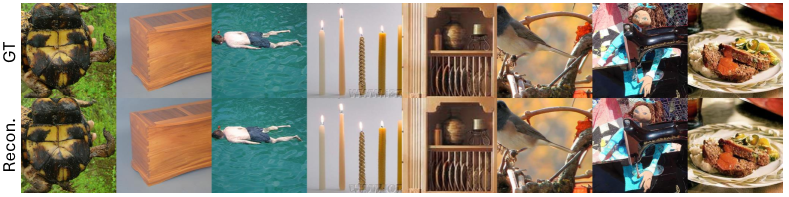
D.4 Generation Results

More visualizations of SiT-XL trained on SoftVQ-L with 32 and 64 tokens are shown here.

Figure 8: Uncurated 256$\times$256 generation results of DiT-XL with SoftVQ-L 64 tokens. We use CFG with 4.0. Class label = ”balloon” (417).

Figure 9: Uncurated 256$\times$256 generation results of DiT-XL with SoftVQ-L 64 tokens. We use CFG with 4.0. Class label = “baseball” (429).

Figure 10: Uncurated 256$\times$256 generation results of DiT-XL with SoftVQ-L 64 tokens. We use CFG with 4.0. Class label = “dog sled” (537).

Figure 11: Uncurated 256$\times$256 generation results of DiT-XL with SoftVQ-L 64 tokens. We use CFG with 4.0. Class label = “space shuttle” (812).

Figure 12: Uncurated 256$\times$256 generation results of DiT-XL with SoftVQ-L 32 tokens. We use CFG with 4.0. Class label = “panda” (388).

Figure 13: Uncurated 256$\times$256 generation results of DiT-XL with SoftVQ-L 32 tokens. We use CFG with 4.0. Class label = “geyser” (974).

Figure 14: Uncurated 256$\times$256 generation results of SiT-XL with SoftVQ-L 64 tokens. We use CFG with 4.0. Class label = “golden retriever” (207).

Figure 15: Uncurated 256$\times$256 generation results of SiT-XL with SoftVQ-L 64 tokens. We use CFG with 4.0. Class label = “arctic wolf” (270).

Figure 16: Uncurated 256$\times$256 generation results of SiT-XL with SoftVQ-L 64 tokens. We use CFG with 4.0. Class label = “lion” (291).

Figure 17: Uncurated 256$\times$256 generation results of SiT-XL with SoftVQ-L 64 tokens. We use CFG with 4.0. Class label = “loggerhead sea turtle” (33).

Figure 18: Uncurated 256$\times$256 generation results of SiT-XL with SoftVQ-L 64 tokens. We use CFG with 4.0. Class label = “fire truck” (555).

Figure 19: Uncurated 256$\times$256 generation results of SiT-XL with SoftVQ-L 64 tokens. We use CFG with 4.0. Class label = “laptop” (620).

Figure 20: Uncurated 256$\times$256 generation results of SiT-XL with SoftVQ-L 64 tokens. We use CFG with 4.0. Class label = “macaw” (88).

Figure 21: Uncurated 256$\times$256 generation results of SiT-XL with SoftVQ-L 64 tokens. We use CFG with 4.0. Class label = “sulphur-crested cockatoo” (89).

Figure 22: Uncurated 256$\times$256 generation results of SiT-XL with SoftVQ-L 64 tokens. We use CFG with 4.0. Class label = “ice cream” (928).

Figure 23: Uncurated 256$\times$256 generation results of SiT-XL with SoftVQ-L 64 tokens. We use CFG with 4.0. Class label = “cheeseburger” (933).

Figure 24: Uncurated 256$\times$256 generation results of SiT-XL with SoftVQ-L 32 tokens. We use CFG with 4.0. Class label = “coral reef” (973).

Figure 25: Uncurated 256$\times$256 generation results of SiT-XL with SoftVQ-L 32 tokens. We use CFG with 4.0. Class label = “lake shore” (975).

Figure 26: Uncurated 512$\times$512 generation results of SiT-XL with SoftVQ-L 64 tokens. We use CFG with 2.0. Class label = “cliff drop-off” (972).

Figure 27: Uncurated 512$\times$512 generation results of SiT-XL with SoftVQ-L 64 tokens. We use CFG with 2.0. Class label = “volcano” (980).

References

- Albergo et al. [2023] Michael S Albergo, Nicholas M Boffi, and Eric Vanden-Eijnden. Stochastic interpolants: A unifying framework for flows and diffusions. arXiv preprint arXiv:2303.08797, 2023.
- Anderson [1982] Brian DO Anderson. Reverse-time diffusion equation models. Stochastic Processes and their Applications, 12(3):313–326, 1982.
- Baevski et al. [2020] Alexei Baevski, Yuhao Zhou, Abdelrahman Mohamed, and Michael Auli. wav2vec 2.0: A framework for self-supervised learning of speech representations. Advances in neural information processing systems, 33:12449–12460, 2020.
- Bao et al. [2023] Fan Bao, Shen Nie, Kaiwen Xue, Yue Cao, Chongxuan Li, Hang Su, and Jun Zhu. All are worth words: A vit backbone for diffusion models. In Proceedings of the IEEE/CVF conference on computer vision and pattern recognition, pages 22669–22679, 2023.
- Bao et al. [2021] Hangbo Bao, Li Dong, Songhao Piao, and Furu Wei. Beit: Bert pre-training of image transformers. arXiv preprint arXiv:2106.08254, 2021.
- Bar-Tal et al. [2024] Omer Bar-Tal, Hila Chefer, Omer Tov, Charles Herrmann, Roni Paiss, Shiran Zada, Ariel Ephrat, Junhwa Hur, Guanghui Liu, Amit Raj, et al. Lumiere: A space-time diffusion model for video generation. arXiv preprint arXiv:2401.12945, 2024.
- Bengio et al. [2013] Yoshua Bengio, Nicholas Léonard, and Aaron Courville. Estimating or propagating gradients through stochastic neurons for conditional computation. arXiv preprint arXiv:1308.3432, 2013.
- Blattmann et al. [2023] Andreas Blattmann, Tim Dockhorn, Sumith Kulal, Daniel Mendelevitch, Maciej Kilian, Dominik Lorenz, Yam Levi, Zion English, Vikram Voleti, Adam Letts, et al. Stable video diffusion: Scaling latent video diffusion models to large datasets. arXiv preprint arXiv:2311.15127, 2023.
- Caron et al. [2021] Mathilde Caron, Hugo Touvron, Ishan Misra, Hervé Jégou, Julien Mairal, Piotr Bojanowski, and Armand Joulin. Emerging properties in self-supervised vision transformers. In Proceedings of the IEEE/CVF international conference on computer vision, pages 9650–9660, 2021.
- Chang et al. [2022] Huiwen Chang, Han Zhang, Lu Jiang, Ce Liu, and William T. Freeman. Maskgit: Masked generative image transformer, 2022.
- Chen et al. [2024a] Junyu Chen, Han Cai, Junsong Chen, Enze Xie, Shang Yang, Haotian Tang, Muyang Li, Yao Lu, and Song Han. Deep compression autoencoder for efficient high-resolution diffusion models. arXiv preprint arXiv:2410.10733, 2024a.
- Chen et al. [2024b] Liang Chen, Haozhe Zhao, Tianyu Liu, Shuai Bai, Junyang Lin, Chang Zhou, and Baobao Chang. An image is worth 1/2 tokens after layer 2: Plug-and-play inference acceleration for large vision-language models. arXiv preprint arXiv:2403.06764, 2024b.
- Chen et al. [2016] Xi Chen, Diederik P Kingma, Tim Salimans, Yan Duan, Prafulla Dhariwal, John Schulman, Ilya Sutskever, and Pieter Abbeel. Variational lossy autoencoder. arXiv preprint arXiv:1611.02731, 2016.
- Chen et al. [2024c] Xinlei Chen, Zhuang Liu, Saining Xie, and Kaiming He. Deconstructing denoising diffusion models for self-supervised learning. arXiv preprint arXiv:2401.14404, 2024c.
- Deng et al. [2009] Jia Deng, Wei Dong, Richard Socher, Li-Jia Li, Kai Li, and Li Fei-Fei. Imagenet: A large-scale hierarchical image database. In 2009 IEEE conference on computer vision and pattern recognition, pages 248–255. Ieee, 2009.
- Dhariwal and Nichol [2021] Prafulla Dhariwal and Alex Nichol. Diffusion models beat gans on image synthesis, 2021.
- Dilokthanakul et al. [2016] Nat Dilokthanakul, Pedro AM Mediano, Marta Garnelo, Matthew CH Lee, Hugh Salimbeni, Kai Arulkumaran, and Murray Shanahan. Deep unsupervised clustering with gaussian mixture variational autoencoders. arXiv preprint arXiv:1611.02648, 2016.
- Ding et al. [2021] Ming Ding, Zhuoyi Yang, Wenyi Hong, Wendi Zheng, Chang Zhou, Da Yin, Junyang Lin, Xu Zou, Zhou Shao, Hongxia Yang, et al. Cogview: Mastering text-to-image generation via transformers. Advances in neural information processing systems, 34:19822–19835, 2021.
- Dong et al. [2023] Xiaoyi Dong, Jianmin Bao, Ting Zhang, Dongdong Chen, Weiming Zhang, Lu Yuan, Dong Chen, Fang Wen, Nenghai Yu, and Baining Guo. Peco: Perceptual codebook for bert pre-training of vision transformers. In Proceedings of the AAAI Conference on Artificial Intelligence, pages 552–560, 2023.
- Dosovitskiy and Brox [2016] Alexey Dosovitskiy and Thomas Brox. Generating images with perceptual similarity metrics based on deep networks. Advances in neural information processing systems, 29, 2016.
- Dosovitskiy et al. [2021] Alexey Dosovitskiy, Lucas Beyer, Alexander Kolesnikov, Dirk Weissenborn, Xiaohua Zhai, Thomas Unterthiner, Mostafa Dehghani, Matthias Minderer, Georg Heigold, Sylvain Gelly, Jakob Uszkoreit, and Neil Houlsby. An image is worth 16x16 words: Transformers for image recognition at scale, 2021.
- Dunn [1973] Joseph C Dunn. A fuzzy relative of the isodata process and its use in detecting compact well-separated clusters. 1973.
- Esser et al. [2021] Patrick Esser, Robin Rombach, and Bjorn Ommer. Taming transformers for high-resolution image synthesis. In Proceedings of the IEEE/CVF conference on computer vision and pattern recognition, pages 12873–12883, 2021.
- Evans et al. [2024] Zach Evans, CJ Carr, Josiah Taylor, Scott H Hawley, and Jordi Pons. Fast timing-conditioned latent audio diffusion. arXiv preprint arXiv:2402.04825, 2024.
- Fan et al. [2024] Lijie Fan, Tianhong Li, Siyang Qin, Yuanzhen Li, Chen Sun, Michael Rubinstein, Deqing Sun, Kaiming He, and Yonglong Tian. Fluid: Scaling autoregressive text-to-image generative models with continuous tokens. arXiv preprint arXiv:2410.13863, 2024.
- Fang et al. [2024] Yuxin Fang, Quan Sun, Xinggang Wang, Tiejun Huang, Xinlong Wang, and Yue Cao. Eva-02: A visual representation for neon genesis. Image and Vision Computing, 149:105171, 2024.
- Fifty et al. [2024] Christopher Fifty, Ronald G Junkins, Dennis Duan, Aniketh Iger, Jerry W Liu, Ehsan Amid, Sebastian Thrun, and Christopher Ré. Restructuring vector quantization with the rotation trick. arXiv preprint arXiv:2410.06424, 2024.
- Gafni et al. [2022] Oran Gafni, Adam Polyak, Oron Ashual, Shelly Sheynin, Devi Parikh, and Yaniv Taigman. Make-a-scene: Scene-based text-to-image generation with human priors. In European Conference on Computer Vision, pages 89–106. Springer, 2022.
- Gao et al. [2023] Shanghua Gao, Pan Zhou, Ming-Ming Cheng, and Shuicheng Yan. Mdtv2: Masked diffusion transformer is a strong image synthesizer. arXiv preprint arXiv:2303.14389, 2023.
- Ge et al. [2023a] Yuying Ge, Yixiao Ge, Ziyun Zeng, Xintao Wang, and Ying Shan. Planting a seed of vision in large language model, 2023a.
- Ge et al. [2023b] Yuying Ge, Sijie Zhao, Ziyun Zeng, Yixiao Ge, Chen Li, Xintao Wang, and Ying Shan. Making llama see and draw with seed tokenizer. arXiv preprint arXiv:2310.01218, 2023b.
- Gong et al. [2022] Shansan Gong, Mukai Li, Jiangtao Feng, Zhiyong Wu, and LingPeng Kong. Diffuseq: Sequence to sequence text generation with diffusion models. arXiv preprint arXiv:2210.08933, 2022.
- Goodfellow et al. [2020] Ian Goodfellow, Jean Pouget-Abadie, Mehdi Mirza, Bing Xu, David Warde-Farley, Sherjil Ozair, Aaron Courville, and Yoshua Bengio. Generative adversarial networks. Communications of the ACM, 63(11):139–144, 2020.
- Gu et al. [2023] Yuchao Gu, Xintao Wang, Yixiao Ge, Ying Shan, Xiaohu Qie, and Mike Zheng Shou. Rethinking the objectives of vector-quantized tokenizers for image synthesis, 2023.
- He et al. [2022] Kaiming He, Xinlei Chen, Saining Xie, Yanghao Li, Piotr Dollár, and Ross Girshick. Masked autoencoders are scalable vision learners. In Proceedings of the IEEE/CVF conference on computer vision and pattern recognition, pages 16000–16009, 2022.
- Heo et al. [2025] Byeongho Heo, Song Park, Dongyoon Han, and Sangdoo Yun. Rotary position embedding for vision transformer. In European Conference on Computer Vision, pages 289–305. Springer, 2025.
- Heusel et al. [2017] Martin Heusel, Hubert Ramsauer, Thomas Unterthiner, Bernhard Nessler, and Sepp Hochreiter. Gans trained by a two time-scale update rule converge to a local nash equilibrium. Advances in Neural Information Processing Systems, 30, 2017.
- Higgins et al. [2017] Irina Higgins, Loic Matthey, Arka Pal, Christopher P Burgess, Xavier Glorot, Matthew M Botvinick, Shakir Mohamed, and Alexander Lerchner. beta-vae: Learning basic visual concepts with a constrained variational framework. ICLR, 3, 2017.
- Hinton and Salakhutdinov [2006] Geoffrey E Hinton and Ruslan R Salakhutdinov. Reducing the dimensionality of data with neural networks. science, 313(5786):504–507, 2006.
- Ho and Salimans [2022] Jonathan Ho and Tim Salimans. Classifier-free diffusion guidance. arXiv preprint arXiv:2207.12598, 2022.
- Ho et al. [2020] Jonathan Ho, Ajay Jain, and Pieter Abbeel. Denoising diffusion probabilistic models. Advances in neural information processing systems, 33:6840–6851, 2020.
- Ho et al. [2022] Jonathan Ho, Tim Salimans, Alexey Gritsenko, William Chan, Mohammad Norouzi, and David J Fleet. Video diffusion models. Advances in Neural Information Processing Systems, 35:8633–8646, 2022.
- Huh et al. [2023] Minyoung Huh, Brian Cheung, Pulkit Agrawal, and Phillip Isola. Straightening out the straight-through estimator: Overcoming optimization challenges in vector quantized networks. In International Conference on Machine Learning, pages 14096–14113. PMLR, 2023.
- Isola et al. [2018] Phillip Isola, Jun-Yan Zhu, Tinghui Zhou, and Alexei A. Efros. Image-to-image translation with conditional adversarial networks, 2018.
- Jegou et al. [2010] Herve Jegou, Matthijs Douze, and Cordelia Schmid. Product quantization for nearest neighbor search. IEEE transactions on pattern analysis and machine intelligence, 33(1):117–128, 2010.
- Johnson et al. [2016a] Justin Johnson, Alexandre Alahi, and Li Fei-Fei. Perceptual losses for real-time style transfer and super-resolution. In Computer Vision–ECCV 2016: 14th European Conference, Amsterdam, The Netherlands, October 11-14, 2016, Proceedings, Part II 14, pages 694–711. Springer, 2016a.
- Johnson et al. [2016b] Matthew J Johnson, David K Duvenaud, Alex Wiltschko, Ryan P Adams, and Sandeep R Datta. Composing graphical models with neural networks for structured representations and fast inference. Advances in neural information processing systems, 29, 2016b.
- Karras et al. [2019] Tero Karras, Samuli Laine, and Timo Aila. A style-based generator architecture for generative adversarial networks. In Proceedings of the IEEE/CVF conference on computer vision and pattern recognition, pages 4401–4410, 2019.
- Karras et al. [2020] Tero Karras, Samuli Laine, Miika Aittala, Janne Hellsten, Jaakko Lehtinen, and Timo Aila. Analyzing and improving the image quality of stylegan. In Proceedings of the IEEE/CVF conference on computer vision and pattern recognition, pages 8110–8119, 2020.
- Kingma and Gao [2024] Diederik Kingma and Ruiqi Gao. Understanding diffusion objectives as the elbo with simple data augmentation. Advances in Neural Information Processing Systems, 36, 2024.
- Kingma [2013] Diederik P Kingma. Auto-encoding variational bayes. arXiv preprint arXiv:1312.6114, 2013.
- Kynkäänniemi et al. [2019] Tuomas Kynkäänniemi, Tero Karras, Samuli Laine, Jaakko Lehtinen, and Timo Aila. Improved precision and recall metric for assessing generative models. Advances in neural information processing systems, 32, 2019.
- Kynkäänniemi et al. [2024] Tuomas Kynkäänniemi, Miika Aittala, Tero Karras, Samuli Laine, Timo Aila, and Jaakko Lehtinen. Applying guidance in a limited interval improves sample and distribution quality in diffusion models. arXiv preprint arXiv:2404.07724, 2024.
- Larsen et al. [2016] Anders Boesen Lindbo Larsen, Søren Kaae Sønderby, Hugo Larochelle, and Ole Winther. Autoencoding beyond pixels using a learned similarity metric. In International conference on machine learning, pages 1558–1566. PMLR, 2016.
- Lee et al. [2022a] Doyup Lee, Chiheon Kim, Saehoon Kim, Minsu Cho, and Wook-Shin Han. Autoregressive image generation using residual quantization. In Proceedings of the IEEE/CVF Conference on Computer Vision and Pattern Recognition, pages 11523–11532, 2022a.
- Lee et al. [2022b] Doyup Lee, Chiheon Kim, Saehoon Kim, Minsu Cho, and Wook-Shin Han. Autoregressive image generation using residual quantization, 2022b.
- Li et al. [2024a] Haopeng Li, Jinyue Yang, Kexin Wang, Xuerui Qiu, Yuhong Chou, Xin Li, and Guoqi Li. Scalable autoregressive image generation with mamba. arXiv preprint arXiv:2408.12245, 2024a.
- Li et al. [2023a] Junnan Li, Dongxu Li, Silvio Savarese, and Steven Hoi. Blip-2: Bootstrapping language-image pre-training with frozen image encoders and large language models. In International conference on machine learning, pages 19730–19742. PMLR, 2023a.
- Li et al. [2023b] Tianhong Li, Huiwen Chang, Shlok Kumar Mishra, Han Zhang, Dina Katabi, and Dilip Krishnan. Mage: Masked generative encoder to unify representation learning and image synthesis, 2023b.
- Li et al. [2024b] Tianhong Li, Yonglong Tian, He Li, Mingyang Deng, and Kaiming He. Autoregressive image generation without vector quantization, 2024b.
- Li et al. [2024c] Wentong Li, Yuqian Yuan, Jian Liu, Dongqi Tang, Song Wang, Jianke Zhu, and Lei Zhang. Tokenpacker: Efficient visual projector for multimodal llm. arXiv preprint arXiv:2407.02392, 2024c.
- Li et al. [2024d] Xiang Li, Hao Chen, Kai Qiu, Jason Kuen, Jiuxiang Gu, Bhiksha Raj, and Zhe Lin. Imagefolder: Autoregressive image generation with folded tokens. arXiv preprint arXiv:2410.01756, 2024d.
- Li et al. [2024e] Yanwei Li, Yuechen Zhang, Chengyao Wang, Zhisheng Zhong, Yixin Chen, Ruihang Chu, Shaoteng Liu, and Jiaya Jia. Mini-gemini: Mining the potential of multi-modality vision language models. arXiv preprint arXiv:2403.18814, 2024e.
- Lin et al. [2023] Ziyi Lin, Chris Liu, Renrui Zhang, Peng Gao, Longtian Qiu, Han Xiao, Han Qiu, Chen Lin, Wenqi Shao, Keqin Chen, et al. Sphinx: The joint mixing of weights, tasks, and visual embeddings for multi-modal large language models. arXiv preprint arXiv:2311.07575, 2023.
- Lipman et al. [2022] Yaron Lipman, Ricky TQ Chen, Heli Ben-Hamu, Maximilian Nickel, and Matt Le. Flow matching for generative modeling. arXiv preprint arXiv:2210.02747, 2022.
- Liu et al. [2024] Wenze Liu, Le Zhuo, Yi Xin, Sheng Xia, Peng Gao, and Xiangyu Yue. Customize your visual autoregressive recipe with set autoregressive modeling. arXiv preprint arXiv:2410.10511, 2024.
- Lloyd [1982] Stuart Lloyd. Least squares quantization in pcm. IEEE transactions on information theory, 28(2):129–137, 1982.
- Loshchilov [2017] I Loshchilov. Decoupled weight decay regularization. arXiv preprint arXiv:1711.05101, 2017.
- Lu and Song [2024] Cheng Lu and Yang Song. Simplifying, stabilizing and scaling continuous-time consistency models. arXiv preprint arXiv:2410.11081, 2024.
- Luo et al. [2024a] Gen Luo, Yiyi Zhou, Yuxin Zhang, Xiawu Zheng, Xiaoshuai Sun, and Rongrong Ji. Feast your eyes: Mixture-of-resolution adaptation for multimodal large language models. arXiv preprint arXiv:2403.03003, 2024a.
- Luo et al. [2024b] Zhuoyan Luo, Fengyuan Shi, Yixiao Ge, Yujiu Yang, Limin Wang, and Ying Shan. Open-magvit2: An open-source project toward democratizing auto-regressive visual generation. arXiv preprint arXiv:2409.04410, 2024b.
- Ma et al. [2024] Nanye Ma, Mark Goldstein, Michael S Albergo, Nicholas M Boffi, Eric Vanden-Eijnden, and Saining Xie. Sit: Exploring flow and diffusion-based generative models with scalable interpolant transformers. arXiv preprint arXiv:2401.08740, 2024.
- Mentzer et al. [2023] Fabian Mentzer, David Minnen, Eirikur Agustsson, and Michael Tschannen. Finite scalar quantization: Vq-vae made simple, 2023.
- MidJourney Inc. [2022] MidJourney Inc. Midjourney. Software available from MidJourney Inc., 2022.
- Nichol and Dhariwal [2021] Alex Nichol and Prafulla Dhariwal. Improved denoising diffusion probabilistic models, 2021.
- Nichol et al. [2021] Alex Nichol, Prafulla Dhariwal, Aditya Ramesh, Pranav Shyam, Pamela Mishkin, Bob McGrew, Ilya Sutskever, and Mark Chen. Glide: Towards photorealistic image generation and editing with text-guided diffusion models. arXiv preprint arXiv:2112.10741, 2021.
- Nyquist [1928] Harry Nyquist. Certain topics in telegraph transmission theory. Transactions of the American Institute of Electrical Engineers, 47(2):617–644, 1928.
- OpenAI [2024] OpenAI. Video generation models as world simulators. OpenAI Blog, 2024.
- Oquab et al. [2023] Maxime Oquab, Timothée Darcet, Theo Moutakanni, Huy V. Vo, Marc Szafraniec, Vasil Khalidov, Pierre Fernandez, Daniel Haziza, Francisco Massa, Alaaeldin El-Nouby, Russell Howes, Po-Yao Huang, Hu Xu, Vasu Sharma, Shang-Wen Li, Wojciech Galuba, Mike Rabbat, Mido Assran, Nicolas Ballas, Gabriel Synnaeve, Ishan Misra, Herve Jegou, Julien Mairal, Patrick Labatut, Armand Joulin, and Piotr Bojanowski. Dinov2: Learning robust visual features without supervision, 2023.
- Peebles and Xie [2023] William Peebles and Saining Xie. Scalable diffusion models with transformers, 2023.
- Popov et al. [2021] Vadim Popov, Ivan Vovk, Vladimir Gogoryan, Tasnima Sadekova, and Mikhail Kudinov. Grad-tts: A diffusion probabilistic model for text-to-speech. In International Conference on Machine Learning, pages 8599–8608. PMLR, 2021.
- Radford et al. [2021] Alec Radford, Jong Wook Kim, Chris Hallacy, Aditya Ramesh, Gabriel Goh, Sandhini Agarwal, Girish Sastry, Amanda Askell, Pamela Mishkin, Jack Clark, et al. Learning transferable visual models from natural language supervision. In International conference on machine learning, pages 8748–8763. PMLR, 2021.
- Ramesh et al. [2021] Aditya Ramesh, Mikhail Pavlov, Gabriel Goh, Scott Gray, Chelsea Voss, Alec Radford, Mark Chen, and Ilya Sutskever. Zero-shot text-to-image generation. In International conference on machine learning, pages 8821–8831. Pmlr, 2021.
- Razavi et al. [2019a] Ali Razavi, Aaron Van den Oord, and Oriol Vinyals. Generating diverse high-fidelity images with vq-vae-2. Advances in neural information processing systems, 32, 2019a.
- Razavi et al. [2019b] Ali Razavi, Aaron van den Oord, and Oriol Vinyals. Generating diverse high-fidelity images with vq-vae-2, 2019b.
- Reynolds et al. [2009] Douglas A Reynolds et al. Gaussian mixture models. Encyclopedia of biometrics, 741(659-663), 2009.
- Rombach et al. [2022a] Robin Rombach, Andreas Blattmann, Dominik Lorenz, Patrick Esser, and Björn Ommer. High-resolution image synthesis with latent diffusion models. In Proceedings of the IEEE/CVF conference on computer vision and pattern recognition, pages 10684–10695, 2022a.
- Rombach et al. [2022b] Robin Rombach, Andreas Blattmann, Dominik Lorenz, Patrick Esser, and Björn Ommer. High-resolution image synthesis with latent diffusion models, 2022b.
- Saharia et al. [2022] Chitwan Saharia, William Chan, Saurabh Saxena, Lala Li, Jay Whang, Emily L Denton, Kamyar Ghasemipour, Raphael Gontijo Lopes, Burcu Karagol Ayan, Tim Salimans, et al. Photorealistic text-to-image diffusion models with deep language understanding. Advances in neural information processing systems, 35:36479–36494, 2022.
- Salimans et al. [2016] Tim Salimans, Ian Goodfellow, Wojciech Zaremba, Vicki Cheung, Alec Radford, and Xi Chen. Improved techniques for training gans. Advances in Neural Information Processing Systems, 29, 2016.
- Shannon [1949] Claude Elwood Shannon. Communication in the presence of noise. Proceedings of the IRE, 37(1):10–21, 1949.
- Sohl-Dickstein et al. [2015a] Jascha Sohl-Dickstein, Eric Weiss, Niru Maheswaranathan, and Surya Ganguli. Deep unsupervised learning using nonequilibrium thermodynamics. In International conference on machine learning, pages 2256–2265. PMLR, 2015a.
- Sohl-Dickstein et al. [2015b] Jascha Sohl-Dickstein, Eric A. Weiss, Niru Maheswaranathan, and Surya Ganguli. Deep unsupervised learning using nonequilibrium thermodynamics, 2015b.
- Song et al. [2024] Dingjie Song, Wenjun Wang, Shunian Chen, Xidong Wang, Michael Guan, and Benyou Wang. Less is more: A simple yet effective token reduction method for efficient multi-modal llms. arXiv preprint arXiv:2409.10994, 2024.
- Song et al. [2022] Jiaming Song, Chenlin Meng, and Stefano Ermon. Denoising diffusion implicit models, 2022.
- stabilityai [2023] stabilityai. Sd vae ft ema, 2023. Accessed: 2023.
- Su et al. [2024] Jianlin Su, Murtadha Ahmed, Yu Lu, Shengfeng Pan, Wen Bo, and Yunfeng Liu. Roformer: Enhanced transformer with rotary position embedding. Neurocomputing, 568:127063, 2024.
- Sun et al. [2024] Peize Sun, Yi Jiang, Shoufa Chen, Shilong Zhang, Bingyue Peng, Ping Luo, and Zehuan Yuan. Autoregressive model beats diffusion: Llama for scalable image generation. arXiv preprint arXiv:2406.06525, 2024.
- Tian et al. [2024] Keyu Tian, Yi Jiang, Zehuan Yuan, Bingyue Peng, and Liwei Wang. Visual autoregressive modeling: Scalable image generation via next-scale prediction, 2024.
- Tschannen et al. [2025] Michael Tschannen, Cian Eastwood, and Fabian Mentzer. Givt: Generative infinite-vocabulary transformers. In European Conference on Computer Vision, pages 292–309. Springer, 2025.
- Tseng et al. [2021] Hung-Yu Tseng, Lu Jiang, Ce Liu, Ming-Hsuan Yang, and Weilong Yang. Regularizing generative adversarial networks under limited data, 2021.
- Vahdat et al. [2021] Arash Vahdat, Karsten Kreis, and Jan Kautz. Score-based generative modeling in latent space, 2021.
- Van den Oord et al. [2016] Aaron Van den Oord, Nal Kalchbrenner, Lasse Espeholt, Oriol Vinyals, Alex Graves, et al. Conditional image generation with pixelcnn decoders. Advances in neural information processing systems, 29, 2016.
- Van Den Oord et al. [2017] Aaron Van Den Oord, Oriol Vinyals, et al. Neural discrete representation learning. Advances in neural information processing systems, 30, 2017.
- Vaswani et al. [2023] Ashish Vaswani, Noam Shazeer, Niki Parmar, Jakob Uszkoreit, Llion Jones, Aidan N. Gomez, Lukasz Kaiser, and Illia Polosukhin. Attention is all you need, 2023.
- Vincent et al. [2008] Pascal Vincent, Hugo Larochelle, Yoshua Bengio, and Pierre-Antoine Manzagol. Extracting and composing robust features with denoising autoencoders. In Proceedings of the 25th international conference on Machine learning, pages 1096–1103, 2008.
- Wang et al. [2024] Xinlong Wang, Xiaosong Zhang, Zhengxiong Luo, Quan Sun, Yufeng Cui, Jinsheng Wang, Fan Zhang, Yueze Wang, Zhen Li, Qiying Yu, et al. Emu3: Next-token prediction is all you need. arXiv preprint arXiv:2409.18869, 2024.
- Weber et al. [2024] Mark Weber, Lijun Yu, Qihang Yu, Xueqing Deng, Xiaohui Shen, Daniel Cremers, and Liang-Chieh Chen. Maskbit: Embedding-free image generation via bit tokens. arXiv preprint arXiv:2409.16211, 2024.
- Wu et al. [2024] Yecheng Wu, Zhuoyang Zhang, Junyu Chen, Haotian Tang, Dacheng Li, Yunhao Fang, Ligeng Zhu, Enze Xie, Hongxu Yin, Li Yi, et al. Vila-u: a unified foundation model integrating visual understanding and generation. arXiv preprint arXiv:2409.04429, 2024.
- Xie et al. [2024] Jinheng Xie, Weijia Mao, Zechen Bai, David Junhao Zhang, Weihao Wang, Kevin Qinghong Lin, Yuchao Gu, Zhijie Chen, Zhenheng Yang, and Mike Zheng Shou. Show-o: One single transformer to unify multimodal understanding and generation. arXiv preprint arXiv:2408.12528, 2024.
- Yu et al. [2021] Jiahui Yu, Xin Li, Jing Yu Koh, Han Zhang, Ruoming Pang, James Qin, Alexander Ku, Yuanzhong Xu, Jason Baldridge, and Yonghui Wu. Vector-quantized image modeling with improved vqgan. arXiv preprint arXiv:2110.04627, 2021.
- Yu et al. [2023] Lijun Yu, José Lezama, Nitesh B Gundavarapu, Luca Versari, Kihyuk Sohn, David Minnen, Yong Cheng, Vighnesh Birodkar, Agrim Gupta, Xiuye Gu, et al. Language model beats diffusion–tokenizer is key to visual generation. arXiv preprint arXiv:2310.05737, 2023.
- Yu et al. [2024a] Lijun Yu, Yong Cheng, Zhiruo Wang, Vivek Kumar, Wolfgang Macherey, Yanping Huang, David Ross, Irfan Essa, Yonatan Bisk, Ming-Hsuan Yang, et al. Spae: Semantic pyramid autoencoder for multimodal generation with frozen llms. Advances in Neural Information Processing Systems, 36, 2024a.
- Yu et al. [2024b] Qihang Yu, Ju He, Xueqing Deng, Xiaohui Shen, and Liang-Chieh Chen. Randomized autoregressive visual generation. arXiv preprint arXiv:2411.00776, 2024b.
- Yu et al. [2024c] Qihang Yu, Mark Weber, Xueqing Deng, Xiaohui Shen, Daniel Cremers, and Liang-Chieh Chen. An image is worth 32 tokens for reconstruction and generation. arxiv: 2406.07550, 2024c.
- Yu et al. [2024d] Sihyun Yu, Sangkyung Kwak, Huiwon Jang, Jongheon Jeong, Jonathan Huang, Jinwoo Shin, and Saining Xie. Representation alignment for generation: Training diffusion transformers is easier than you think. arXiv preprint arXiv:2410.06940, 2024d.
- Zeghidour et al. [2021] Neil Zeghidour, Alejandro Luebs, Ahmed Omran, Jan Skoglund, and Marco Tagliasacchi. Soundstream: An end-to-end neural audio codec. IEEE/ACM Transactions on Audio, Speech, and Language Processing, 30:495–507, 2021.
- Zhang et al. [2024] Baoquan Zhang, Huaibin Wang, Chuyao Luo, Xutao Li, Guotao Liang, Yunming Ye, Xiaochen Qi, and Yao He. Codebook transfer with part-of-speech for vector-quantized image modeling. In Proceedings of the IEEE/CVF Conference on Computer Vision and Pattern Recognition, pages 7757–7766, 2024.
- Zhang et al. [2019] Han Zhang, Zizhao Zhang, Augustus Odena, and Honglak Lee. Consistency regularization for generative adversarial networks. arXiv preprint arXiv:1910.12027, 2019.
- Zhang et al. [2018] Richard Zhang, Phillip Isola, Alexei A. Efros, Eli Shechtman, and Oliver Wang. The unreasonable effectiveness of deep features as a perceptual metric, 2018.
- Zhao et al. [2020] Shengyu Zhao, Zhijian Liu, Ji Lin, Jun-Yan Zhu, and Song Han. Differentiable augmentation for data-efficient gan training. Advances in neural information processing systems, 33:7559–7570, 2020.
- Zheng et al. [2023] Lin Zheng, Jianbo Yuan, Lei Yu, and Lingpeng Kong. A reparameterized discrete diffusion model for text generation. arXiv preprint arXiv:2302.05737, 2023.
- Zhou et al. [2024] Chunting Zhou, Lili Yu, Arun Babu, Kushal Tirumala, Michihiro Yasunaga, Leonid Shamis, Jacob Kahn, Xuezhe Ma, Luke Zettlemoyer, and Omer Levy. Transfusion: Predict the next token and diffuse images with one multi-modal model. arXiv preprint arXiv:2408.11039, 2024.
- Zhu et al. [2024a] Lei Zhu, Fangyun Wei, Yanye Lu, and Dong Chen. Scaling the codebook size of vqgan to 100,000 with a utilization rate of 99%. arXiv preprint arXiv:2406.11837, 2024a.
- Zhu et al. [2010] X Zhu, W Su, L Lu, B Li, X Wang, and J Dai. Deformable detr: Deformable transformers for end-to-end object detection. arxiv 2020. arXiv preprint arXiv:2010.04159, 2010.
- Zhu et al. [2024b] Yongxin Zhu, Bocheng Li, Yifei Xin, and Linli Xu. Addressing representation collapse in vector quantized models with one linear layer. arXiv preprint arXiv:2411.02038, 2024b.