TinySubNets: An efficient and low capacity continual learning strategy

Abstract

Continual Learning (CL) is a highly relevant setting gaining traction in recent machine learning research. Among CL works, architectural and hybrid strategies are particularly effective due to their potential to adapt the model architecture as new tasks are presented. However, many existing solutions do not efficiently exploit model sparsity, and are prone to capacity saturation due to their inefficient use of available weights, which limits the number of learnable tasks. In this paper, we propose TinySubNets (TSN), a novel architectural CL strategy that addresses the issues through the unique combination of pruning with different sparsity levels, adaptive quantization, and weight sharing. Pruning identifies a subset of weights that preserve model performance, making less relevant weights available for future tasks. Adaptive quantization allows a single weight to be separated into multiple parts which can be assigned to different tasks. Weight sharing between tasks boosts the exploitation of capacity and task similarity, allowing for the identification of a better trade-off between model accuracy and capacity. These features allow TSN to efficiently leverage the available capacity, enhance knowledge transfer, and reduce computational resources consumption. Experimental results involving common benchmark CL datasets and scenarios show that our proposed strategy achieves better results in terms of accuracy than existing state-of-the-art CL strategies. Moreover, our strategy is shown to provide a significantly improved model capacity exploitation. Code released at: https://github.com/lifelonglab/tinysubnets.

Adaptive quantization and non-linear quantization

Algorithm 1 showcases the adaptive quantization process. The procedure begins by applying non-linear quantization to the task-pruned model using minimal values for the parameters $\omega$ (number of centroids) and $\psi$ (bit-width) (line 1). This initial step utilizes the non-linear quantization algorithm described in Algorithm 2. Following the quantization, the model’s accuracy is evaluated (line 2). If the accuracy drop exceeds a predefined threshold $\delta$ (line 3), an iterative process is initiated to incrementally increase the bit-width (lines 4-7). This adjustment continues until the accuracy loss is within acceptable limits.

0: $\psi$ – Initial bit-width

0: $Q_{q}$ – Model accuracy

0: $\Theta$ – Pruned model

0: $\delta$ – Maximum loss in accuracy

1: $\Theta_{q},K$ = nonlinear_quantization($\psi,\Theta$) {see Algorithm 2}

2: $Q_{q}$ = acc($F$, $\Theta_{q})$

3: while $Q_{q}$ $<$ $Q$ - $\delta$ do

4:  $\psi$ = $\psi$ + 1

5:  $\Theta_{q},K$ = nonlinear_quantization($\psi,\Theta$)

6:  $Q_{q}$ = acc($F$, $\Theta_{q})$

7: return  $\psi$ – optimal bit-width for the task, $\Theta_{q}$ – quantized model, $K$ – codebook

Algorithm 1 Adaptive Quantization for task $t$.

0: $\psi$ – desired bit-width

0: $\Theta$ – weights of a model

1: $\omega\leftarrow 2^{\psi}$ {Number of centroids}

2: $K\leftarrow[K_{0},K_{1},\dots,K_{|\Theta|}];K_{i}=\{\}$ {Empty codebook}

3: $\Theta^{\prime}\leftarrow$ copy of $\Theta$

4: for $\theta_{i}$ in $\Theta$ do

5:  $C,A\leftarrow$ KMeans($\theta_{i}$, $\omega$) {$C$: centroids, $A$: weight-to-centroid-index assignment}

6:  for $\theta_{i,j}\in\theta_{i}$ do

7:   $\theta^{\prime}_{i,j}\leftarrow A[\theta_{i,j}]$ {Use centroid index instead of weight value}

8:  for $c_{k}\in C$ do

9:   $K_{i}[k]\leftarrow c_{k}$ {Building layer-wise codebook}

10: return  $\Theta^{\prime},K$

Algorithm 2 Non-linear quantization

This adaptive approach ensures that the quantized model maintains a performance close to the original model while optimizing memory usage. By incrementally increasing the bit-width only when necessary, the algorithm finds a balance between model size and accuracy, making it effective for scenarios with strict memory constraints.

Algorithm 2 presents our adopted non-linear quantization approach, which was inspired by (Pietron et al. 2019). The process begins with identifying the number of centroids $\omega$ and creating an empty codebook $K$ to store the mapping between codes and weight values for each layer (lines 1-2). Additionally, we generate a copy of the model $\Theta$, where the weights will contain codes from the codebook (centroid indices) instead of actual values.

The next step involves clustering the weight values of each layer $\theta_{i}$ using the K-Means clustering algorithm, with a specified number of clusters ($\omega$) (line 5). This step produces two outputs: a list of centroids $C$ and a list of weight-to-centroid-index assignments $A$. Each weight is then assigned its corresponding centroid index (lines 6-8).

To maintain the mapping between centroid indices and centroids, a codebook is constructed for each layer (lines 9-11). The algorithm ultimately returns the model copy with quantized weights, now represented as codes from the codebook, and the codebook that is essential for converting the codes back to their actual weight values.

It is important to note that the number of centroids is directly related to the desired bit-width (as indicated in line 1). Fewer centroids result in reduced memory requirements for storing the weights, as each weight is stored as an index of its closest centroid. This approach ensures that memory usage is minimized while retaining the essential information needed for the model’s performance.

Formal details

Pruning is defined as a function:

$$P:\theta_{i}\rightarrow{\theta_{i}^{\prime}},\theta_{i}^{\prime}=M_{i}\odot\theta_{i}$$ (1)

where: $M_{i}$ is a binary matrix with bits assigned to single weights

$$\sum_{m\in M_{i}}M_{i}=\Upsilon_{i}$$ (2)

Quantization assigns centroids to weights:

$$Q:\theta_{i}\rightarrow Y_{K_{i}},Y_{K_{i}}\equiv\min\forall_{Y_{K_{i}}}|Y_{K_{i}}-\theta_{i}|$$ (3)

$$K_{i}:X\rightarrow Y,X\in\mathbb{Z}\land Y\in\mathbb{R}$$ (4)

$$|X|=2^{\phi_{t}}$$ (5)

The equation for accuracy loss can be defined as:

$$\mathcal{L}_{(x,y)}=\mathcal{L}_{ce}(Y,F_{Q(P(\Theta))})+\sum_{i=0}^{L}\mathcal{L}_{mse}(\overline{f_{Q(P(\theta_{i}))}},f_{Q(P(\theta_{i}))})$$ (6)

Kullback-Leibler for computing tasks divergence is defined as:

$$D_{KL}(D_{t}||D_{t-1})=P(D_{t})\cdot\frac{P(D_{t})}{Q(D_{t-1})}$$ (7)

Huffman encoding and decoding

Each tasks binary mask is represented as binary matrix. Each value indicates if weight is used (value 1) or not used by the task (value 0). It is just sparse matrix with nonzero 1 values. Therefore each mask can be compressed. In presented approach mask is encoded using huffman algorithm. The most frequent sub-sequences with their probabilities are are extracted. Then mask is represented as a tree and the dictionary in which mapping is stored (pairs with sequence in original mask and its corresponding code). When mask is loaded the decoding process is run to receive original mask.

Decoding quantized weights

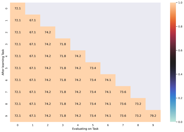
Figure 2: Accuracy matrix for CIFAR100 (TSN-wr)

The quantized weights are encoded in following manner (from fig.2):

• bank

• prefix (which indicates to which task weight belongs to)

• quantized weight value in the codebook

Example: 0 00 11 represents the value -0.3576 (weight $w_{0,1,3}$ in layer 1 and task 1, see fig.2a)

Case study

In this subsection we describe more in detail an example of how TinySubNetworks manages memory capacity, as shown in Figure LABEL:fig:algorithm (with weight sharing, without replay memory, task 1, 2 and 3 share the weights, TSN-wr):

• Original model has capacity in bits: $CAP_{L_{1}}$ = $6\cdot 32b$, $CAP_{L_{2}}$ = $6\cdot 32b$, $\rightarrow$ $384b$.

• After pruning of task 1 capacity: $4$ weights in first layer and $4$ in second layer, after pruning and quantization of task 1: $CAP_{t1}=4\cdot 2b+4\cdot 2b+136b\rightarrow 152b$.

• After pruning of task 2 capacity: it adds $1$ weight in first layer and $1$ weight in second layer, after pruning and quantization of task 2: $CAP_{t2}=152b+2*1b+66b\rightarrow 220b$.

• Task 3 uses weights added by second task and shares some subset of weights from task 1: $CAP_{t3}=220b$.

Hyperparameter optimization

In regards to hyperparameter optimization and overfitting, we resorted to basic heuristics for suitable values for most hyperparameters. Regarding the adaptive pruning process, after the learning process for a given task is completed, the global consolidated mask is updated, and codebook are updated. This process leverages a validation set in order to prevent overfitting. Moreover, sparsity levels in Algorithm 2 are optimized resorting to a greedy non-gradient fine-tuning approach, which does not incur in overfitting issues.

Additional results

In this subsection, we present different results that highlight specific aspects of our method. Results in Table 1 show that the capacity occupation in different scenarios for the compressed model. Masks and weights are a small portion of the original model (after pruning and quantization). Size of the codebooks is negligible.

In Table 2 sparsity before and after fine tuning is shown. In last column the optimal bit-width is reported. Results in Table 3 show that a significantly high model accuracy can be achieved even with a very small number of bits for the quantized model (between 3 and 5 bits).

Results in Table 4 report the execution time for each scenario (training, and fine-tuning), which depends on the specific input size of each dataset, the model backbone, and the batch size. An interesting result is that, while CIFAR100 is a larger dataset than p-MNIST, its execution time is less due to the specific batch size configuration used in our experiments ($2048$ vs. $256$).

A different view on capacity is shown in results in Table 5 (please note that results with replay memory include the memory occupation for the additional memory bank for each task - see Figure LABEL:fig:algorithm). Overall, we observe that post-pruning can reduce the memory footprint of the model. Its impact is particularly high with 5 Datasets (from $30.62\%$ to $24.68\%$). We can also observe that replay memory requires a consistent amount of capacity.

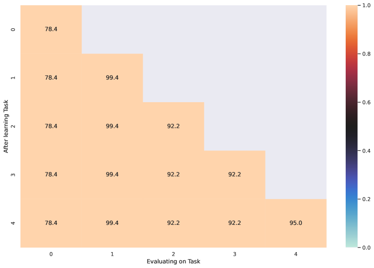
Figure 4: Accuracy matrix for 5 datasets (TSN-wr)

Results in Tables 6 and 7 allow us to highlight that the reduction in FLOPs provided by compression incurs a negligible accuracy loss. For instance, in the TinyImagenet scenario, 8 bit quantization allows to reduce from 4 775M FLOPs to 530.5M (or 450.9M with the pruning variant) at just 0.27 in accuracy drop. In Table 7 the accuracy after centroids quantization and activations quantization is described (in <4b, 4b>, <8b, 8b> and <16b, 16b> formats). It can be observed that in <8b, 8b> and <16b, 16b> configurations the accuracy is still at the same level. In case of <4b, 4b> there is a drop in accuracy. All these configurations can reduce number of FLOPs as it is shown in fig. 4. Note: Floating-point operations <flp, flp> have approximately 9× to 10× of the complexity of <8b, 8b> since there is 3× of the number of bits to represent the mantissas plus the remaining work required to handle exponents.

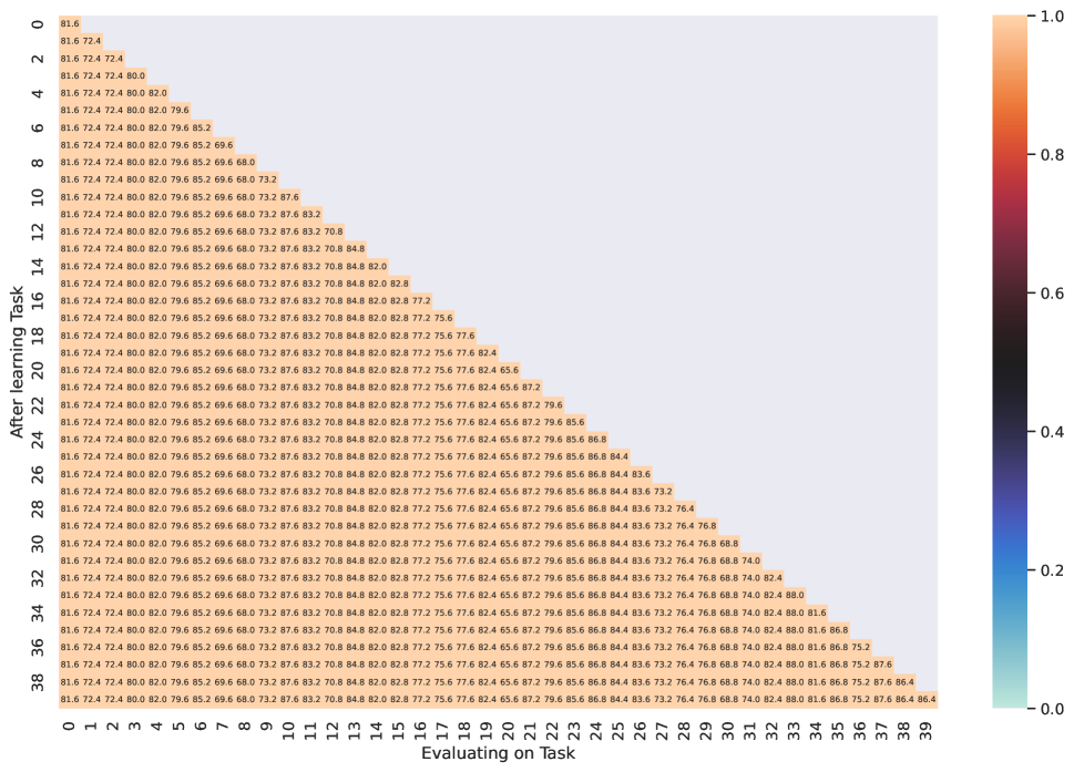
Figure 5: Accuracy matrix for TinyImagenet (TSN-wr)

Forward and Backward Transfer are relevant metrics in continual learning. Results in Table 8 and Figures 2-5 show zero Backward Transfer for all scenarios, which is expected given the forget-free capabilities of the proposed method. As for Forward Transfer, values should be compared to the performance of a random classifier considering the number of classes in each dataset. Overall, we observe that Forward Transfer performance is close to or slightly above random. However, a proper evaluation of this metric is cumbersome in a task-incremental setting, given that our method requires knowledge of the task identifier to create masks and the specific sub-network for each task.

Heatmaps in Figures 2-5 provide additional disaggregated information, showing model performance on each task. It can be observed that the performance varies significantly depending on the task (e.g., on Imagenet-100, the performance varies from $68.9\%$ in task 5 to $83.8\%$ in task 7). The heatmaps further highlight the forget-free capabilities of the method, as shown by the performance on each task which is constant and preserved throughout the entire scenario.

Comparison with WSN and Ada-Q-Packnet

While we recognize that our proposed approach is inspired by the best features of WSN (Kang et al. 2022) (weight sharing) and Ada-QPacknet (Pietron et al. 2023) (pruning and quantization), we did not simply adopt these features. Instead, we developed more effective versions of the same, and devised our own method to synergically combine them.

While Ada-QPacknet (Pietron et al. 2023) adopts compression techniques like pruning and quantization to deal with model capacity, it presents some significant differences with respect to our proposed approach.

First, Ada-QPacknet does not support weight sharing between tasks. This is a significant drawback in the presence of scenarios with high task similarity (similar data distribution), since it incurs in an inefficient use of memory.

Second, our approach to pruning and quantization is different. Specifically, instead of a lottery ticket search as in Ada-QPacknet, our pruning step involves gradient mask optimization and post-training fine-tuning (without gradient), which is also unique when compared to Winning SubNetworks (WSN).

Third, our approach leverages the Kullbach-Leibler Divergence to measure the differences in task distributions, which is a missing feature in both Ada-QPacknet and WSN.

Quantitative comparison with NPCL and QDI

Regarding NPCL (Jha et al. 2024), the authors leverage a ResNet-18 model backbone across all class incremental experiments and two-layer fully connected network for task incremental (p-MNIST). In contrast, we adopt model backbones that are significantly smaller than Resnet-18 for most class incremental scenarios: a reduced AlexNet variant (s-CIFAR100), and TinyNet (TinyImagenet), whereas we adopt Resnet-18 only for the two most complex scenarios (5 datasets and Imagenet100). In case of task incremental we are using similar achitecture: a 2-layer neural network with fully connected layers (p-MNIST). Nevertheless, we are able to achieve a better performance in terms of accuracy in all these scenarios. A comparison of the experimental results show that our method outperforms NPCL in terms of Accuracy in different scenarios: S-CIFAR-100 (77.27 vs. 71.34), TinyImagenet (80.10 vs. 60.18), and p-MNIST (97.14 vs. 95.97).

As for QDI (Madaan et al. 2023), model backbones adopted in the paper are comparable to ours. Comparing the results shows that our method outperforms QDI on TinyImagenet (80.10 vs. 66.79) and QDI outperforms our method on s-CIFAR100 (77.27 vs. 88.30). However, one important consideration is that the setup used for TinyImagenet is 10 tasks with 20 classes, whereas our setting is 40 tasks with 5 classes. At the same time, the setup used in QDI for s-CIFAR100 presents 20 tasks with 5 classes, whereas in our work we consider 10 tasks with 10 classes. Moreover, considering accuracy in isolation may lead to a reductive analysis. A potential pitfall in the QDI paper is that there is no discussion (or empirical analysis) about model capacity (NPCL runs the models with similar size but there is no additional step of capacity reduction). This makes it difficult to gauge the trade-off between accuracy and memory impact of the method, which is one of our distinctive goals.

It is also worth noting that NPCL (Jha et al. 2024) and QDI (Madaan et al. 2023) papers did not provide experiments with the two most complex scenarios (5 datasets and Imagenet100) considered in our study, where our method achieves a remarkable performance.

Ablation analysis

In regards to model capacity, our findings reveal that our pruning step, which involves weight sharing, is directly responsible for reducing memory footprint. As a result, comparing our approach to Ada-QPacknet and WSN leads to a significant improvement in capacity (e.g. from $81.25\%$ and $77.73\%$ to $22.65\%$ for p-MNIST – other examples are presented in Table 1). We argue that in case of Ada-QPacknet the quantization step contributes to model capacity to a lesser degree than adaptive pruning, since the bit-width achieved in our experiments is comparable to Ada-QPacknet (Pietron et al. 2023). The quantization step contributes significantly when we try to compare TSN with WSN (WSN has no reduction stage for the bit-width of the parameters and activations). Fine-tuning just minimally contributes to model capacity.

As for model accuracy, we argue that performance gains are obtained thanks to our pruning approach with dynamic masks updated during the training process. This approach provides a significant improvement over other methods where masks are statically initialized, such as Ada-QPacknet (see Table 2).

Open challenges

As for potential limitations of the proposed approach, we envision that if the divergence between tasks is too high (low inter-task similarity) adaptive pruning may struggle to identify suitable shared weights, leading to memory saturation to accommodate all tasks. This possible limitation can be also identified in other continual learning methods such as WSN (Kang et al. 2022) and Ada-QPacknet (Pietron et al. 2023). Similar considerations can be drawn for very long scenarios (e.g. characterized by hundreds of tasks). In this particular case, adaptive pruning could be less effective, and quantization is expected to be the main driver for memory reduction. In general, future research is required to assess the robustness of continual learning methods in very complex scenarios.

Table 1: Memory capacity results for codebooks, masks and weights (including pruning and quantized values).

Scenarios	weights	codebooks	masks
p-MNIST	9.8%	< 0.1%	12.5%
CIFAR100	5.49 %	< 0.1%	12.5%
5 datasets	14.57%	< 0.1%	10%
TinyImagenet	12.5%	< 0.1%	20%
Imagenet100	12.5%	< 0.1%	12,5%

Table 2: Sparsity and bit widths for different benchmarks.

Scenarios	sparsity before fine tuning	sparsity after fine tuning	bit-width
p-MNIST	37.58	41.2	4 bits
CIFAR100	7.22	11.68	4 bits
5 datasets	1.02	21.02	4 bits
TinyImagenet	2.7	14.31	5 bits
Imagenet100	8.5	10.1	5 bits

Table 3: Accuracy results for different weight bit width.

Scenarios	5 bits	4 bits	3 bits
p-MNIST	96.85	96.63	96.06
CIFAR100	74.82	75.14	75.07
TinyImagenet	77.19	77.16	68.01
5 Datasets	91.71	91.80	90.1

Table 4: Average execution times on single GPU for different benchmarks (in seconds).

Scenarios	training time [s]	fine tuning time [s]
p-MNIST	1 244	23.92
CIFAR100	662	12.6
TinyImagenet	6752	122.76
Imagenet100	5 094	84.9

Table 5: Comparison of capacity with and without post-pruning (post-pruning run with 100 iterations), and with replay memory.

Scenarios	without post-pruning	with post-pruning	with replay memory
p-MNIST	23.41%	22.65%	37.5%*
CIFAR100	18.75%	17.62%	41.92%
TinyImagenet	36.33%	32.15%	93.6%
5 Datasets	30.62%	24.68%	40.08%

Table 6: Number of FLOPs in case of floating point and with reduced bit-width of both weights and activations.

Scenarios	4 bit + p	8 bit + p	16 bit + p	4 bit	8 bit	16 bit	baseline floating-point
p-MNIST	0.97M	3.89M	15.6M	1.62M	6.5M	26M	61.7M
CIFAR100	214.37M	857.5M	3 430M	243.6M	974.4M	3 897M	8 770M
TinyImagenet	112.72M	450.9M	1 803M	132.62M	530.5M	2 122M	4 775M

Table 7: Accuracy with reduced bit-width of activations and quantized centroids.

Scenarios	4 bit	8 bit	16 bit
p-MNIST	84.08	97.06	97.13
CIFAR100	70.86	75.21	75.46
TinyImagenet	75.84	79.66	79.70
5 Datasets	85.2	91.71	91.78

Table 8: Forward and Backward Transfer for TSN

Scenarios	Backward Transfer	Forward Transfer
p-MNIST	0.0	0.104
CIFAR100	0.0	0.010
TinyImagenet	0.0	0.004
5 Datasets	0.0	-
Imagenet100	0.0	-

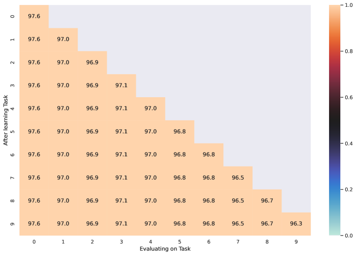
Figure 1: Accuracy matrix for p-MNIST (TSN-wr)

Figure 3: Accuracy matrix for Imagenet-100 (TSN-wr)

References

- Jha et al. (2024) Jha, S.; Gong, D.; Zhao, H.; and Yao, L. 2024. NPCL: Neural Processes for Uncertainty-Aware Continual Learning. Advances in Neural Information Processing Systems, 36.
- Kang et al. (2022) Kang, H.; Mina, R. J. L.; Rizky, S.; Madjid, H.; Yoon, J.; Hasegawa-Johnson, M.; Ju-Hwang, S.; and Yoo, C. D. 2022. Forget-free Continual Learning with Winning Subnetworks. ICML, x.
- Madaan et al. (2023) Madaan, D.; Yin, H.; Byeon, W.; Kautz, J.; and Molchanov, P. 2023. Heterogeneous continual learning. In Proceedings of the IEEE/CVF Conference on Computer Vision and Pattern Recognition, 15985–15995.
- Pietron et al. (2019) Pietron, M.; Karwatowski, M.; Wielgosz, M.; and Duda, J. 2019. Fast Compression and Optimization of Deep Learning Models for Natural Language Processing. 162–168.
- Pietron et al. (2023) Pietron, M.; Zurek, D.; Faber, K.; and Corizzo, R. 2023. Ada-QPacknet – Multi-Task Forget-Free Continual Learning with Quantization Driven Adaptive Pruning. In 26th European Conference on Artificial Intelligence, ECAI 2023, 1882–1889.