Posterior asymptotics of high-dimensional spiked covariance model with inverse-Wishart prior

Abstract

We consider Bayesian inference on the spiked eigenstructures of high-dimensional covariance matrices; specifically, we focus on estimating the eigenvalues and corresponding eigenvectors of high-dimensional covariance matrices in which a few eigenvalues are significantly larger than the rest. We impose an inverse-Wishart prior distribution on the unknown covariance matrix and derive the posterior distributions of the eigenvalues and eigenvectors by transforming the posterior distribution of the covariance matrix. We prove that the posterior distribution of the spiked eigenvalues and corresponding eigenvectors converges to the true parameters under the spiked high-dimensional covariance assumption, and also that the posterior distribution of the spiked eigenvector attains the minimax optimality under the single spiked covariance model. Simulation studies and real data analysis demonstrate that our proposed method outperforms all existing methods in quantifying uncertainty.

1 Introduction

Covariance matrix estimation is a crucial component of multivariate analysis, as the covariance matrix represents the dependencies between variables. The sample covariance matrix is a widely used estimator for the covariance; however, it becomes singular when the number of variables exceeds the number of observations. Moreover, Yin et al. (1988) and Bai et al. (2007) demonstrated that the eigenvalues and eigenvectors of the sample covariance matrix may fail to converge to the true parameters in high-dimensional settings. To address this issue, structural assumptions are often imposed on the covariance matrix in high-dimensional contexts. For instance, Cai and Zhou (2010) and Lee et al. (2023) explored banded or bandable covariance matrices, while Cai et al. (2013) and Lee and Lee (2023) focused on sparse covariance matrices.

In this paper, we consider the spiked assumption for the covariance matrix. The spiked assumption posits that a small number of eigenvalues are substantially larger than the others. Under this assumption, the total variation in the data is predominantly explained by variations along the directions of the spiked eigenvectors of the covariance matrix. We focus on estimating these spiked eigenvalues and their corresponding eigenvectors.

Johnstone and Lu (2009) examined the asymptotic properties of the sample eigenvector for a single spiked covariance matrix $\displaystyle\bm{\Sigma}=\nu_{p}\bm{\xi}_{p}\bm{\xi}_{p}^{\top}+\bm{I}_{p}$, where $\displaystyle\nu_{p}>0$ and $\displaystyle\bm{\xi}_{p}\in\mathbb{S}^{p-1}$, with $\displaystyle\mathbb{S}^{p-1}=\{\bm{x}\in\mathbb{R}^{p}:||\bm{x}||_{2}=1\}$. The first eigenvalue of $\displaystyle\bm{\Sigma}$ is $\displaystyle\nu_{p}+1$, and the corresponding eigenvector is $\displaystyle\bm{\xi}_{p}$. Johnstone and Lu (2009) showed that the first sample eigenvector is consistent if and only if $\displaystyle p/n\longrightarrow 0$ under the assumption that $\displaystyle\nu_{p}$ is bounded above by a positive constant. Furthermore, the minimax lower bound for the estimation of $\displaystyle\bm{\xi}_{p}$ is $\displaystyle\min\Big{\{}\frac{1+\nu_{p}}{\nu_{p}^{2}}\frac{p}{n},1\Big{\}}$ (see Example 15.19 in Wainwright (2019)). Thus, a divergence condition on the spiked eigenvalue or an additional structural assumption is required for the consistent estimation of the spiked eigenvector under the high-dimensional setting.

In high-dimensional spiked covariance models, sparse assumptions on the elements of the eigenvectors were considered by Johnstone and Lu (2009), Amini et al. (2009), and Ma et al. (2013), among others. On the other hand, divergent conditions on the spiked eigenvalues were examined by Fan et al. (2013), Wang and Fan (2017), and Cai et al. (2020), among others. Fan et al. (2013) introduced the pervasiveness condition in the statistical factor model to establish when the divergent condition applies in real data analysis. Under the divergent condition, Wang and Fan (2017) and Cai et al. (2020) examined the asymptotic properties of sample eigenvalues and eigenvectors in high-dimensional settings.

We explore Bayesian inference of the spiked covariance matrix under a divergent condition on the spiked eigenvalues, without imposing structural assumptions such as sparsity or bandedness. Bayesian inference on the spiked eigenvalues and eigenvectors of the covariance matrix has been studied in the context of principal component analysis and factor models. Bishop (1998) proposed Bayesian principal component analysis using the factor analysis model with isotropic Gaussian noise, but this method is not shown to be consistent in high-dimensional settings. Ma and Liu (2022) considered the high-dimensional setting for the Bayesian factor model, imposing a sparsity assumption on the loading matrix, implying that the principal directions involve only a small subset of variables. Although the method by Ma and Liu (2022) is shown to be consistent in high-dimensional settings, the sparsity assumption restricts its applicability in many real-world scenarios. Zhong et al. (2022) proposes an empirical Bayes estimator for principal component analysis. Although Zhong et al. (2022) considers the high-dimensional setting without the sparsity assumption, they provide only a posterior mean estimator, lacking interval estimation.

In this paper, we propose a Bayesian method to estimate the spiked eigenvalues and their corresponding eigenvectors using an inverse-Wishart prior distribution. First, we impose an inverse-Wishart prior distribution on the covariance matrix and derive its posterior distribution. Next, we derive the posterior distribution of the spiked eigenstructure, comprising the spiked eigenvalues and their corresponding eigenvectors. Sampling from the inverse-Wishart distribution is straightforward, making the posterior computation of the proposed method efficient.

We study the asymptotic properties of the inverse-Wishart posterior for estimating spiked eigenvalues and eigenvectors. Previous research on the asymptotic analysis of spiked eigenvalues and eigenvectors has primarily focused on the sample eigenvalues and eigenvectors, as seen in works by Johnstone and Lu (2009), Wang and Fan (2017), and Cai et al. (2020). The sample covariance matrix has rank $\displaystyle n$ when $\displaystyle p>n$, and the asymptotic analysis of sample eigenvalues and eigenvectors in high-dimensional settings relies on the low rank of the sample covariance. However, extending the asymptotic analysis of sample covariance to the posterior contraction rate is not straightforward, as the posterior samples of the covariance matrix are full-rank matrices. Thus, we develop concentration inequalities for random spiked eigenvalues and eigenvectors without assuming a low-rank covariance matrix and apply these inequalities to the inverse-Wishart distribution. We also prove the minimax optimality of the posterior distribution of the spiked eigenvector under the single spiked covariance model.

Our contributions are as follows: first, we have proposed a Bayesian method for the spiked eigenstructure, which offers several advantages: (1) it is theoretically justified in the high-dimensional setting, (2) it does not impose a sparsity assumption, (3) it is computationally straightforward, and (4) it quantifies uncertainty in the estimates. Second, we have developed concentration inequalities of spiked eigenvalues and eigenvectors, thereby reducing the convergence analysis of spiked eigenvalue and eigenvector estimators to that of the covariance estimator with respect to the spectral norm.

The rest of the paper is organized as follows. In Section 2.1, we introduce the spiked covariance model. Section 2.2 presents the Bayesian method for estimating the spiked eigenstructure. In Section 3, the concentration inequalities and the posterior contraction rate are presented. In Section 4, we illustrate the proposed method through a simulation study and real data analysis. The concluding remarks are given in Section 5. We provide the proofs of theorems, corollaries and propositions in Section 6 and the Appendix section.

2 Bayesian inference in spiked covariance model

2.1 Spiked covariance model

Suppose $\displaystyle\bm{X}_{1},\ldots,\bm{X}_{n}$ are random samples from a $\displaystyle p$-dimensional multivariate normal distribution $\displaystyle N_{p}(\bm{0}_{p},\bm{\Sigma})$, where $\displaystyle\bm{\Sigma}\in\mathcal{C}_{p}$ and $\displaystyle\mathcal{C}_{p}$ is the set of all $\displaystyle p\times p$ positive definite matrices. Let $\displaystyle\lambda_{1}\geq\ldots\geq\lambda_{p}>0$ be the eigenvalues of $\displaystyle\bm{\Sigma}$, and let $\displaystyle\bm{\xi}_{1},\ldots,\bm{\xi}_{p}$ be the corresponding eigenvectors. The covariance matrix $\displaystyle\bm{\Sigma}$ is referred to as a spiked covariance when the top $\displaystyle K$ eigenvalues are much larger than the remaining ones; that is, $\displaystyle\lambda_{1}\geq\ldots,\lambda_{K}>>\lambda_{K+1}\geq\ldots\geq\lambda_{p}$.

In particular, we consider the following model:

$$\displaystyle\bm{X}_{1},\ldots,\bm{X}_{n} \displaystyle\sim \displaystyle N_{p}(\bm{0},\bm{\Sigma}),$$ (1)

$$\displaystyle\frac{\lambda_{K+1}p}{\lambda_{K}n} \displaystyle\longrightarrow \displaystyle 0,$$ (2)

$$\displaystyle\frac{K^{3}}{n} \displaystyle\longrightarrow \displaystyle 0,$$ (3)

$$\displaystyle\frac{\lambda_{k}}{\lambda_{k+1}} \displaystyle> \displaystyle C,~k=1,\ldots,K$$ (4)

for some positive constant $\displaystyle C>1$.

Condition (4) assumes that the top $\displaystyle K$ eigenvalues are well-separated. Condition (2) ensures that the top eigenvalues dominate relative to $\displaystyle\lambda_{K+1}p/n$. In other words, if $\displaystyle\lambda_{K+1}p/n$ is small, the top eigenvalues need not be large; however, if $\displaystyle\lambda_{K+1}p/n$ is large, they must exceed $\displaystyle\lambda_{K+1}p/n$ significantly. The additional condition on $\displaystyle K$ in (3) allows for a regime of a growing number of spiked eigenvalues. Conditions (2) and (3) are less restrictive than Assumption 2 in Cai et al. (2020), in which $\displaystyle\lambda_{K+1}$ is bounded, $\displaystyle\frac{p}{n\lambda_{K}}\longrightarrow 0$, and $\displaystyle\frac{K^{6}}{n}\longrightarrow 0$.

The condition (2) requires the spiked eigenvalue to diverge when $\displaystyle\lambda_{K+1}p\gtrsim n$, and Fan et al. (2013) introduced the pervasiveness condition to demonstrate the practicality of the divergent condition in the context of the statistical factor model. We describe the factor model and the pervasiveness condition below, demonstrating that the pervasiveness condition ensures condition (2). Suppose a $\displaystyle p$-dimensional observation $\displaystyle\bm{X}$ is explained by $\displaystyle K$ unobserved factors $\displaystyle\bm{f}=(f_{1},\ldots,f_{K})^{T}\in\mathbb{R}^{K}$ and can be represented by

$$\bm{X}\mid\bm{f} = \sum_{k=1}^{K}\bm{b}_{k}f_{k}+\bm{\epsilon},$$ (5)

$$\bm{f} \sim N_{K}(\bm{0}_{K},\bm{I}_{K}),$$

$$\bm{\epsilon} \sim N_{p}(\bm{0}_{p},\bm{\Sigma}_{u}),$$

where $\displaystyle\bm{b}_{k}\in\mathbb{R}^{p}$ quantifies the effect of the $\displaystyle k$th factor $\displaystyle f_{k}$ on the observation $\displaystyle\bm{X}$, and $\displaystyle\bm{\epsilon}$ represents the error of $\displaystyle\bm{X}$ that is not explained by the factors. By integrating out $\displaystyle f_{1},\ldots,f_{K}$, the observation $\displaystyle\bm{X}$ follows a multivariate normal distribution $\displaystyle N_{p}(\bm{0}_{p},\bm{B}\bm{B}^{T}+\bm{\Sigma}_{u})$, where $\displaystyle\bm{B}=(\bm{b}_{1},\ldots,\bm{b}_{K})\in\mathbb{R}^{p\times K}$. Additionally, we suppose the columns of $\displaystyle\bm{B}$ are orthogonal, which is the canonical condition for the identifiability (see Proposition 2.1 in Fan et al. (2013)).

If $\displaystyle||\bm{\Sigma}_{u}||_{2}$ is bounded and $\displaystyle||\bm{b}_{k}||_{2}^{2}$ diverges at a rate of at least $\displaystyle p$ as $\displaystyle p\longrightarrow\infty$, i.e., $\displaystyle\liminf_{p\longrightarrow\infty}||\bm{b}_{k}||_{2}^{2}/p>0$, $\displaystyle k=1,\ldots,K$, we say that the factor model (5) satisfies the pervasiveness condition (see Assumption 2.1 in Fan et al. (2021)), which means that the factor $\displaystyle f_{k}$ affects a substantial proportion of the variation in the observations. Without loss of generality, we suppose $\displaystyle||\bm{b}_{1}||_{2}\geq\ldots\geq||\bm{b}_{K}||_{2}$. Since $\displaystyle\lambda_{k}(\bm{\Sigma})\geq\lambda_{k}(\bm{B}\bm{B}^{T})=||\bm{b}_{k}||_{2}^{2}$, $\displaystyle k=1,\ldots,K$, and $\displaystyle\lambda_{K+1}(\bm{\Sigma})\leq||\bm{\Sigma}_{u}||_{2}$, the pervasiveness condition yields $\displaystyle\frac{\lambda_{0,K+1}p}{\lambda_{0,K}n}\leq\frac{||\bm{\Sigma}_{u}||_{2}p}{||\bm{b}_{K}||_{2}^{2}n}\lesssim 1/n$, which implies (2).

2.2 Bayesian inference of eigenvalues and eigenvectors with inverse-Wishart prior

We propose a Bayesian method for the inference of the spiked eigenstructure of the covariance matrix, i.e., we consider the model (1) with assumptions (2)-(4). First, we impose an inverse-Wishart prior distribution $\displaystyle\bm{\Sigma}\sim IW_{p}(\bm{A}_{n},\nu_{n})$ on the covariance matrix, whose density function is

$$\pi(\bm{\Sigma})\propto|\bm{\Sigma}|^{-(\nu_{n}+p+1)/2}\exp\{-\textup{tr}(\bm{\Sigma}^{-1}\bm{A}_{n})/2\},$$

where $\displaystyle\nu_{n}>2p$ is the degree of freedom, $\displaystyle\bm{A}_{n}$ is a $\displaystyle p\times p$ positive definite matrix, and $\displaystyle|\bm{\Sigma}|$ denotes the determinant of $\displaystyle\bm{\Sigma}$.

By the conjugacy of the inverse-Wishart prior, we obtain the posterior distribution $\displaystyle\bm{\Sigma}\mid\mathbb{X}_{n}\sim IW_{p}(\bm{A}_{n}+\sum_{i=1}^{n}\bm{X}_{i}\bm{X}_{i}^{T},\nu_{n}+n)$, where $\displaystyle\mathbb{X}_{n}$ denotes the set of $\displaystyle n$ observations $\displaystyle\bm{X}_{1},\ldots,\bm{X}_{n}$. From the posterior distribution of $\displaystyle\bm{\Sigma}$, we can efficiently compute the posterior distributions of the top $\displaystyle K$ eigenvalues and eigenvectors, $\displaystyle[\lambda_{k}(\bm{\Sigma})\mid\mathbb{X}_{n}]$ and $\displaystyle[\bm{\xi}_{k}(\bm{\Sigma})\mid\mathbb{X}_{n}]$, $\displaystyle k=1,\ldots,K$, where $\displaystyle[X\mid Y]$ denotes the conditional distribution of $\displaystyle X$ given $\displaystyle Y$, $\displaystyle\lambda_{k}(\cdot):\mathcal{C}_{p}\mapsto\mathbb{R}$, and $\displaystyle\bm{\xi}_{k}(\cdot):\mathcal{C}_{p}\mapsto\mathbb{R}^{p}$ are the operators that yield the $\displaystyle k$-th largest eigenvalue and its eigenvector, respectively.

The algorithm for generating posterior samples from $\displaystyle[\lambda_{k}(\bm{\Sigma})\mid\mathbb{X}_{n}]$ and $\displaystyle[\bm{\xi}_{k}(\bm{\Sigma})\mid\mathbb{X}_{n}]$ is given below:

1. Independently generate $\displaystyle\bm{\Sigma}_{1},\ldots,\bm{\Sigma}_{N}\sim IW(\bm{A}_{n}+\sum_{i=1}^{n}\bm{X}_{i}\bm{X}_{i}^{T},\nu_{n}+n)$.

2. Compute the $\displaystyle k$-th eigenvalue and eigenvectors of $\displaystyle\bm{\Sigma}_{1},\ldots,\bm{\Sigma}_{N}$ and obtain

   $$\displaystyle\lambda_{k}(\bm{\Sigma}_{1}),\ldots,\lambda_{k}(\bm{\Sigma}_{N}),$$

   $$\displaystyle\bm{\xi}_{k}(\bm{\Sigma}_{1}),\ldots,\bm{\xi}_{k}(\bm{\Sigma}_{N}),$$

   for $\displaystyle k=1,\ldots,K$.

Note that the posterior samples $\displaystyle(\lambda_{k}(\bm{\Sigma}_{1}),\ldots,\lambda_{k}(\bm{\Sigma}_{N}))$ and $\displaystyle(\bm{\xi}_{k}(\bm{\Sigma}_{1}),\ldots,\bm{\xi}_{k}(\bm{\Sigma}_{N}))$ obtained through the algorithm are used to approximate the posterior distributions $\displaystyle[\lambda_{k}(\bm{\Sigma})\mid\mathbb{X}_{n}]$ and $\displaystyle[\bm{\xi}_{k}(\bm{\Sigma})\mid\mathbb{X}_{n}]$, respectively. The algorithm is straightforward to implement, as it only requires inverse Wishart sampling and spectral decomposition. Furthermore, since the posterior samples are independent, there is no need for convergence diagnostics of Markov chains.

3 Posterior contraction rate

3.1 Posterior contraction rate of spiked eigenvalues

In this section, we provide the posterior contraction rate of $\displaystyle[\lambda_{k}(\bm{\Sigma})\mid\mathbb{X}_{n}]$. The posterior contraction rate is an asymptotic property of the posterior distribution to describe how quickly the posterior distribution contracts around the true parameter. A sequence $\displaystyle\epsilon_{n}$ is a posterior contraction rate at the parameter $\displaystyle\theta_{0}$ with respect to the loss function $\displaystyle d:\Theta\times\Theta\mapsto\mathbb{R}^{+}$ if $\displaystyle\pi(\theta:d(\theta,\theta_{0})\geq M_{n}\epsilon_{n}\mid\mathbb{X}_{n})\longrightarrow 0$ in $\displaystyle\mathbb{P}(\mathbb{X}_{n};\theta_{0})$-probability, for every $\displaystyle M_{n}\longrightarrow\infty$. See Ghosal and Van der Vaart (2017). In this section, we let $\displaystyle[K]$ denote $\displaystyle\{1,\ldots,K\}$ for an integer $\displaystyle K$. Given any positive sequences $\displaystyle a_{n}$ and $\displaystyle b_{n}$, we denote $\displaystyle a_{n}=o(b_{n})$ if $\displaystyle a_{n}/b_{n}\longrightarrow 0$ as $\displaystyle n\longrightarrow\infty$, and $\displaystyle a_{n}\lesssim b_{n}$ if there exists a constant $\displaystyle C>0$ such that $\displaystyle a_{n}\leq Cb_{n}$ for all sufficiently large $\displaystyle n$.

We provide Theorem 3.1, which provides a concentration inequality for the top $\displaystyle k$ eigenvalues. The deviation probability of eigenvalues, $\displaystyle P\left(\sup_{l=1,\ldots,k}\left|\frac{\lambda_{l}(\bm{\Sigma})}{\lambda_{0,l}}-1\right|>Ct\right)$, is bounded by the sum of the deviation probabilities for $\displaystyle||\bm{\Gamma}_{\perp}^{T}\bm{\Sigma}_{0}^{-1/2}\bm{\Sigma}\bm{\Sigma}_{0}^{-1/2}\bm{\Gamma}_{\perp}||_{2}$ and $\displaystyle||\bm{\Gamma}^{T}\bm{\Sigma}_{0}^{-1/2}\bm{\Sigma}\bm{\Sigma}_{0}^{-1/2}\bm{\Gamma}-\bm{I}_{K}||_{2}$. Therefore, it is sufficient to analyze the concentration inequalities of the scaled covariance matrix $\displaystyle\bm{\Sigma}_{0}^{-1/2}\bm{\Sigma}\bm{\Sigma}_{0}^{-1/2}$ to investigate the asymptotic property of the eigenvalues.

Theorem 3.1.

Suppose $\displaystyle\bm{\Sigma}$ is a positive definite random matrix, $\displaystyle\bm{\Sigma}_{0}\in\mathcal{C}_{p}$ is a fixed positive definite matrix, and $\displaystyle K\in[p]$. Let $\displaystyle\lambda_{0,1}\geq\ldots\geq\lambda_{0,p}>0$ be eigenvalues of $\displaystyle\bm{\Sigma}_{0}$ and $\displaystyle\bm{u}_{0,1},\ldots,\bm{u}_{0,p}$ be the corresponding eigenvectors. Let $\displaystyle\bm{\Gamma}=[\bm{u}_{0,1},\ldots,\bm{u}_{0,K}]$ and $\displaystyle\bm{\Gamma}_{\perp}=[\bm{u}_{0,K+1},\ldots,\bm{u}_{0,p}]$. Suppose $\displaystyle\min_{l=1,\ldots,K-1}\frac{\lambda_{0,l}}{\lambda_{0,l+1}}>c$ with $\displaystyle c>1$, and let $\displaystyle k\in[K]$. Then,

$$\displaystyle P(\sup_{l=1,\ldots,k}|\frac{\lambda_{l}(\bm{\Sigma})}{\lambda_{0,l}}-1|>Ct) \displaystyle\leq \displaystyle P(||\bm{\Gamma}_{\perp}^{T}\bm{\Sigma}_{0}^{-1/2}\bm{\Sigma}\bm{\Sigma}_{0}^{-1/2}\bm{\Gamma}_{\perp}||^{1/2}\frac{\sqrt{\lambda_{0,K+1}}}{\sqrt{\lambda_{0,k}}}>t)$$

$$\displaystyle+P(K||\bm{\Gamma}^{T}\bm{\Sigma}_{0}^{-1/2}\bm{\Sigma}\bm{\Sigma}_{0}^{-1/2}\bm{\Gamma}-\bm{I}_{K}||_{2}>t),$$

for all $\displaystyle t\leq\delta$, where $\displaystyle\delta$ and $\displaystyle C$ are some positive constants dependent on $\displaystyle c$.

The proof is given in the Appendix B

Applying Theorem 3.1, we obtain Corollary 3.2, which establishes the contraction rate of the inverse-Wishart posterior distribution. The posterior contraction rate of the top $\displaystyle k$ eigenvalues is given as

$$\epsilon_{n}=\sqrt{\frac{K^{3}}{n}}+\sqrt{\frac{\lambda_{0,K+1}}{\lambda_{0,k}}}\Big{(}\sqrt{\frac{p}{n}}\vee 1\Big{)}.$$

The conditions on $\displaystyle K$, $\displaystyle\lambda_{0,k}$, and $\displaystyle\lambda_{0,K+1}$ for consistency are less restrictive than Assumptions 2 and $\displaystyle 2^{\prime}$ in Cai et al. (2020). Theorem 2.1 with Assumptions 2 and $\displaystyle 2^{\prime}$ in Cai et al. (2020) requires $\displaystyle K^{6}/n=o(1)$, $\displaystyle\frac{p}{n\lambda_{0,k}}=o(1)$, and that $\displaystyle\lambda_{0,K+1}$ is bounded.

Corollary 3.2.

Suppose $\displaystyle\bm{X}_{1},\ldots,\bm{X}_{n}\sim N(\bm{0}_{p},\bm{\Sigma}_{0})$, and $\displaystyle\bm{\Sigma}_{0}$ satisfies (2) and (4). Consider the inverse-Wishart prior distribution $\displaystyle\bm{\Sigma}\sim IW_{p}(\bm{A}_{n},\nu_{n})$. Let $\displaystyle\lambda_{0,1}\geq\ldots\geq\lambda_{0,p}$ be the eigenvalues of $\displaystyle\bm{\Sigma}_{0}$. Let $\displaystyle k\in[K]$ and $\displaystyle\epsilon_{n}^{2}=K^{3}/n+\frac{\lambda_{0,K+1}}{\lambda_{0,k}}\Big{(}\frac{p}{n}\vee 1\Big{)}$. If $\displaystyle p/n^{2}=o(1)$, $\displaystyle||\bm{\Sigma}_{0}^{-1/2}\bm{A}_{n}\bm{\Sigma}_{0}^{-1/2}||_{2}=o(n)$, $\displaystyle\nu_{n}-p=o(n)$, $\displaystyle K^{3}=o(n)$, and $\displaystyle\frac{\lambda_{0,K+1}}{\lambda_{0,k}}\Big{(}\frac{p}{n}\vee 1\Big{)}=o(1)$, then

$$\displaystyle\pi(\sup_{l=1,\ldots,k}|\frac{\lambda_{l}(\bm{\Sigma})}{\lambda_{0,l}}-1|>M_{n}\epsilon_{n}\mid\mathbb{X}_{n})$$

converges to $\displaystyle 0$ in probability for arbitrary positive real valued sequence $\displaystyle M_{n}$ with $\displaystyle M_{n}\longrightarrow\infty$.

The proof is given in the Appendix C.

3.2 Posterior contraction rate of spiked eigenvectors

To investigate the posterior contraction rate of $\displaystyle[\bm{\xi}_{k}(\bm{\Sigma})\mid\mathbb{X}_{n}]$, we provide Theorem 3.3, which provides concentration inequalities for eigenvectors with respect to the loss function $\displaystyle 1-(\bm{u}^{T}\bm{u}_{0})^{2}$, the square of the sine distance of the pair of unit vectors $\displaystyle\bm{u}$ and $\displaystyle\bm{u}_{0}$. The loss function quantifies the directional discrepancy without accounting for the sign. The deviation probability for eigenvectors, $\displaystyle P\left(\sup_{l=1,\ldots,k}\{1-(\bm{u}_{l}^{T}\bm{u}_{0,l})^{2}\}>Ct\right)$, is bounded by the sum of the deviation probabilities for $\displaystyle||\bm{\Gamma}_{\perp}^{T}\bm{\Sigma}_{0}^{-1/2}\bm{\Sigma}\bm{\Sigma}_{0}^{-1/2}\bm{\Gamma}_{\perp}||_{2}$ (or $\displaystyle||\bm{\Sigma}_{0}^{-1/2}\bm{\Sigma}\bm{\Sigma}_{0}^{-1/2}-\bm{I}_{p}||_{2}$), $\displaystyle||\bm{\Gamma}^{T}\bm{\Sigma}_{0}^{-1/2}\bm{\Sigma}\bm{\Sigma}_{0}^{-1/2}\bm{\Gamma}-\bm{I}_{K}||_{2}$, and the spiked eigenvalues. Thus, as in Theorem 3.1, it suffices to consider the concentration inequalities of the scaled covariance matrix $\displaystyle\bm{\Sigma}_{0}^{-1/2}\bm{\Sigma}\bm{\Sigma}_{0}^{-1/2}$ to investigate the asymptotic property of the eigenvectors. As shown in Theorem 3.1, the deviation probability of the spiked eigenvalues can also be derived from the concentration inequalities for $\displaystyle\bm{\Sigma}_{0}^{-1/2}\bm{\Sigma}\bm{\Sigma}_{0}^{-1/2}$. In Theorem 3.3, two versions of the concentration inequalities are given as (6) and (7), which are used in the proof of the following corollary for the cases $\displaystyle p>n$ and $\displaystyle p\leq n$, respectively.

Theorem 3.3.

Suppose $\displaystyle\bm{\Sigma}$ is a positive definite random matrix, $\displaystyle\bm{\Sigma}_{0}$ is a fixed positive definite matrix, and $\displaystyle K\in[p]$. Let $\displaystyle\lambda_{0,1}\geq\ldots\geq\lambda_{0,p}>0$ be eigenvalues of $\displaystyle\bm{\Sigma}_{0}$ and $\displaystyle\bm{u}_{0,1},\ldots,\bm{u}_{0,p}$ be the corresponding eigenvectors. Also, $\displaystyle\lambda_{1}\geq\ldots\geq\lambda_{p}>0$ be eigenvalues of $\displaystyle\bm{\Sigma}$ and $\displaystyle\bm{u}_{1},\ldots,\bm{u}_{p}$ be the corresponding eigenvectors. Let $\displaystyle\bm{\Gamma}=[\bm{u}_{0,1},\ldots,\bm{u}_{0,K}]$, $\displaystyle\bm{\Gamma}_{\perp}=[\bm{u}_{0,K+1},\ldots,\bm{u}_{0,p}]$, $\displaystyle k\in[K]$ and $\displaystyle B_{k}=\sup_{l=1,\ldots,k}\{(\sup_{i\leq l-1}\lambda_{0,l}/\lambda_{0,i})\vee(\sup_{i\geq l+1}\lambda_{0,i}/\lambda_{0,l})\}$. Suppose $\displaystyle\min_{l=1,\ldots,K-1}\frac{\lambda_{0,l}}{\lambda_{0,l+1}}>c$ with $\displaystyle c>1$ and $\displaystyle\frac{\lambda_{0,K+1}}{\lambda_{k}}\leq d$ with $\displaystyle d<1$. Then,

$$\displaystyle P(\sup_{l=1,\ldots,k}\{1-(\bm{u}_{l}^{T}\bm{u}_{0,l})^{2}\}>Ct) \displaystyle\leq \displaystyle P(||\bm{\Gamma}_{\perp}^{T}\bm{\Sigma}_{0}^{-1/2}\bm{\Sigma}\bm{\Sigma}_{0}^{-1/2}\bm{\Gamma}_{\perp}||_{2}^{1/2}\frac{\sqrt{\lambda_{0,K+1}}}{\sqrt{\lambda_{0,k}}}>\sqrt{t})$$ (6)

$$\displaystyle+P(||\bm{\Gamma}^{T}\bm{\Sigma}_{0}^{-1/2}\bm{\Sigma}\bm{\Sigma}_{0}^{-1/2}\bm{\Gamma}-\bm{I}_{K}||_{2}>\frac{\sqrt{t}}{\sqrt{B_{k}}}\wedge\delta_{2})$$

$$\displaystyle+P(\sup_{l=1,\ldots,k}|\frac{\lambda_{l}}{\lambda_{0,l}}-1|>\delta_{1}),$$

and

$$\displaystyle P(\sup_{l=1,\ldots,k}\{1-(\bm{u}_{l}^{T}\bm{u}_{0,l})^{2}\}>Ct) \displaystyle\leq \displaystyle P(||\bm{\Sigma}_{0}^{-1/2}\bm{\Sigma}\bm{\Sigma}_{0}^{-1/2}-\bm{I}_{p}||_{2}^{1/2}\frac{\sqrt{\lambda_{0,K+1}}}{\sqrt{\lambda_{0,k}}}>\sqrt{t})$$ (7)

$$\displaystyle+P(||\bm{\Gamma}^{T}\bm{\Sigma}_{0}^{-1/2}\bm{\Sigma}\bm{\Sigma}_{0}^{-1/2}\bm{\Gamma}-\bm{I}_{K}||_{2}>\frac{\sqrt{t}}{\sqrt{B_{k}}}\wedge\delta_{2})$$

$$\displaystyle+P(\sup_{l=1,\ldots,k}|\frac{\lambda_{l}}{\lambda_{0,l}}-1|>\delta_{1}),$$

for all $\displaystyle t\leq\delta$, where $\displaystyle C$, $\displaystyle\delta_{1}$, $\displaystyle\delta_{2}$ and $\displaystyle\delta$ are some positive constant dependent on $\displaystyle c$ and $\displaystyle d$.

The proof is given in Section 6.

Applying Theorem 3.3, we obtain Corollary 3.4, which establishes the posterior contraction rate for the top $\displaystyle K$ eigenvectors, expressed as

$$\frac{B_{k}K}{n}+\frac{\lambda_{0,K+1}}{\lambda_{0,k}}\frac{p}{n}.$$

Corollary 3.4 ensures uniform convergence over the top $\displaystyle k$ eigenvalues, whereas Theorem 3.2 in Wang and Fan (2017) and Theorem 4.1 in Cai et al. (2020) do not.

Corollary 3.4.

Suppose the same setting as in Corollary 3.2. Let $\displaystyle B_{k}=\sup_{l=1,\ldots,k}\{(\sup_{i\leq l-1}\lambda_{0,l}/\lambda_{0,i})\vee(\sup_{i\geq l+1}\lambda_{0,i}/\lambda_{0,l})\}$ and $\displaystyle\epsilon_{n}=\frac{B_{k}K}{n}+\frac{\lambda_{0,K+1}}{\lambda_{k}}\frac{p}{n}$. If $\displaystyle p/n^{2}=o(1)$, $\displaystyle||\bm{\Sigma}_{0}^{-1/2}\bm{A}_{n}\bm{\Sigma}_{0}^{-1/2}||_{2}=o(n)$, $\displaystyle\nu_{n}-p=o(n)$, $\displaystyle K^{3}=o(n)$ and $\displaystyle\frac{\lambda_{0,K+1}}{\lambda_{0,k}}\Big{(}\frac{p}{n}\vee 1\Big{)}=o(1)$, then

$$\displaystyle\pi(\sup_{l=1,\ldots,k}\{1-(\bm{\xi}_{l}(\bm{\Sigma})^{T}\bm{\xi}_{l}(\bm{\Sigma}_{0}))^{2}\}>M_{n}\epsilon_{n}\mid\mathbb{X}_{n})$$

converges to $\displaystyle 0$ in probability for any positive sequence $\displaystyle M_{n}$ with $\displaystyle M_{n}\longrightarrow\infty$.

The proof is given in the Appendix D.

The posterior contraction rate achieves minimax optimality for the single spiked covariance model $\displaystyle\bm{\Sigma}_{0}=\nu_{p}\bm{\xi}_{p}\bm{\xi}_{p}^{T}+\bm{I}_{p}$, where $\displaystyle\bm{\xi}_{p}\in\mathbb{S}^{p-1}$ and $\displaystyle\nu_{p}>0$. The eigenvalues of $\displaystyle\bm{\Sigma}_{0}$ are $\displaystyle\lambda_{0,1}=\nu_{p}+1$ and $\displaystyle\lambda_{0,2}=\cdots=\lambda_{0,p}=1$, and the first eigenvector is $\displaystyle\bm{\xi}_{p}$. Corollary 3.4 with $\displaystyle K=1$ and $\displaystyle k=1$ gives the posterior contraction rate for the first eigenvector as $\displaystyle\frac{1+p}{(\nu_{p}+1)n}$, and is asymptotically equivalent to the minimax lower bound stated in Proposition 3.5.

Proposition 3.5.

Suppose $\displaystyle\bm{X}_{1},\ldots,\bm{X}_{n}$ are independent samples from $\displaystyle N_{p}(\bm{0}_{p},\nu_{p}\bm{\xi}_{p}\bm{\xi}_{p}^{T}+\bm{I}_{p})$. Let $\displaystyle\hat{\bm{\xi}}_{p}$ denote an eigenvector estimator. Then, the minimax lower bound is given as

$$\displaystyle\inf_{\hat{\bm{\xi}}_{p}}\sup_{\bm{\xi}_{p}\in\mathbb{S}^{p-1}}E(1-(\hat{\bm{\xi}}_{p}^{T}\bm{\xi}_{p})^{2})\gtrsim\min\Big{\{}\frac{1+\nu_{p}}{\nu_{p}^{2}}\frac{p}{n},1\Big{\}}.$$

The proof is given in the Appendix E.

Remark 3.6.

The Davis-Kahan theorem has been used for the convergence analysis of an eigenvector estimator, especially when the eigenvector is not obtained from the sample covariance (Zwald and Blanchard, 2005; Wei and Minsker, 2017; Han and Liu, 2018). The Davis-Kahan theorem provides the following upper bound:

$$\displaystyle\sin(\bm{v}_{j},\hat{\bm{v}}_{j})\leq\frac{2||\hat{\bm{\Sigma}}-\bm{\Sigma}||_{2}}{\min(\lambda_{j-1}-\lambda_{j},\lambda_{j}-\lambda_{j+1})},$$ (8)

where $\displaystyle\lambda_{j}$ and $\displaystyle\bm{v}_{j}$ are the $\displaystyle j$th eigenvalue and eigenvector of $\displaystyle\bm{\Sigma}$, respectively, and $\displaystyle\hat{\bm{v}}_{j}$ is the $\displaystyle j$th eigenvector of $\displaystyle\hat{\bm{\Sigma}}$ (see Corollary 3 in Yu et al. (2015)). This inequality is used to establish the consistency of $\displaystyle\sin(\bm{v}_{j},\hat{\bm{v}}_{j})$ through the convergence analysis of its upper bound in (8). However, the inequality (8) is not tight enough when the spiked eigenvalues vary in scale. For instance, suppose $\displaystyle\lambda_{1}=p^{2}$, $\displaystyle\lambda_{2}=p$, $\displaystyle\lambda_{3}=\ldots=\lambda_{p}=1$, and $\displaystyle p\geq n$ in model (1). Since $\displaystyle||\hat{\bm{\Sigma}}-\bm{\Sigma}||_{2}\geq|\lambda_{1}-\bm{v}_{1}^{T}\hat{\bm{\Sigma}}\bm{v}_{1}|=\lambda_{1}|\bm{v}_{1}^{T}\bm{\Sigma}^{-1/2}\hat{\bm{\Sigma}}\bm{\Sigma}^{-1/2}\bm{v}_{1}-1|$ and $\displaystyle\inf_{\hat{\bm{\Sigma}}}\sup_{\bm{\Sigma}}E|\bm{v}_{1}^{T}\bm{\Sigma}^{-1/2}\hat{\bm{\Sigma}}\bm{\Sigma}^{-1/2}\bm{v}_{1}-1|\gtrsim 1/\sqrt{n}$ under the Gaussian model (Lee and Lee, 2018), we have

$$\displaystyle\inf_{\hat{\bm{\Sigma}}}\sup_{\bm{\Sigma}}E\Big{[}\frac{2||\hat{\bm{\Sigma}}-\bm{\Sigma}||_{2}}{\min(\lambda_{j-1}-\lambda_{j},\lambda_{j}-\lambda_{j+1})}\Big{]} \displaystyle\gtrsim \displaystyle\frac{\lambda_{1}}{\min(\lambda_{j-1}-\lambda_{j},\lambda_{j}-\lambda_{j+1})}\frac{1}{\sqrt{n}}$$

$$\displaystyle\gtrsim \displaystyle\frac{p}{\sqrt{n}},~\textup{when }j=2.$$

Thus, the right-hand side of (8) fails to converge to $\displaystyle 0$ when $\displaystyle j=2$. However, Corollary 3.4 shows that $\displaystyle\sin(\bm{v}_{2},\hat{\bm{v}}_{2})$ converges to $\displaystyle 0$ when $\displaystyle\hat{\bm{v}}_{2}$ is derived from the inverse-Wishart posterior distribution. Thus, the inequality (8) is not tight enough when the spiked eigenvalues have different scales.

4 Numerical studies

4.1 Simulation studies

In this section, we conduct two simulations to assess the proposed method in the high-dimensional data. We examine the estimation of eigenvalues and eigenvectors of the covariance matrix. In all experiments, we focus on the spiked eigenstructure of the high-dimensional covariance matrix with the condition (2) and (4). The code for the proposed method is publicly available at https://github.com/swpark0413/bisec.

4.2 Estimation of eigenvectors and eigenvalues

We estimate the eigenvalues and eigenvectors of a spiked covariance matrix using the proposed method presented in Section 2. Subsequently, we evaluate the accuracy and uncertainty quantification of these eigenvalues and eigenvectors using 100 replicated data sets. Specifically, we compute the relative errors for the leading $\displaystyle k$th eigenvalue, denoted as $\displaystyle\text{err}_{\lambda}:=|\lambda_{k}(\bm{\Sigma})-\lambda_{k}(\bm{\Sigma}_{0})|/\lambda_{k}(\bm{\Sigma}_{0})$, where $\displaystyle\lambda_{k}(\bm{\Sigma})$ represents the estimated leading $\displaystyle k$th eigenvalue of the covariance. For the eigenvector accuracy, we measure $\displaystyle\text{err}_{\bm{\xi}}:=1-(\bm{\xi}_{k}(\bm{\Sigma})^{T}\bm{\xi}_{k}(\bm{\Sigma}_{0}))^{2}$. The point estimates of the Bayesian method are given as the average of the $\displaystyle 1000$ posterior samples. The posterior mean for eigenvectors, which are direction vectors, is calculated using the Grassmann average method (Hauberg et al., 2014). As the interval estimation, we use the 95% credible interval of posteriors for uncertainty estimation, as the frequentist approach cannot be considered. The coverage probability (CP) is measured by determining how often the true parameters of interest fall within credible intervals across 100 replicates.

The synthetic dataset is generated from a multivariate normal distribution $\displaystyle N_{p}(\bm{0},\bm{\Sigma}_{0})$, where the true spiked covariance $\displaystyle\bm{\Sigma}_{0}=\mathbf{B}\mathbf{B}^{T}+\bm{\Sigma}_{u}$ derived by the factor model (5). Each row of loading matrix $\displaystyle\mathbf{B}$ is drawn from the standard multivariate normal distribution with the $\displaystyle k$th column normalized such that $\displaystyle\sqrt{\lambda_{k}}=\sqrt{p/(nc_{k})}$ for $\displaystyle k=1,2,\ldots,K$. Here, we set $\displaystyle K=4$ and $\displaystyle c_{1}=0.001,c_{2}=0.005,c_{3}=0.01$, and $\displaystyle c_{4}=0.02$ to define the spiked eigenstructure of covariance with conditions 2 and 4. We also assume $\displaystyle\bm{\Sigma}_{u}=\text{diag}(\sigma_{1}^{2},\ldots,\sigma^{2}_{p})$, where each $\displaystyle\sigma_{i}$’s are generated from a $\displaystyle\text{Gamma}(a,b)$ distribution with $\displaystyle a=2$ and $\displaystyle b=5$. For the high-dimensional setting, we set the number of observations to 50 and the number of variables to 100, 200, 500, and 1000. As the hyperparameter of the inverse-Wishart distribution, we set $\displaystyle\bm{A}_{n}=I_{p}$ and $\displaystyle\nu_{n}=p+1$. Here, we assume the number of factors $\displaystyle K$ is known and this assumption is applied across all the methods.

We compared our proposed estimator against the sample covariance (SCOV) as a reference estimator, as well as two Bayesian approaches: Variational Bayesian PCA (VBPCA) introduced by Bishop (1999) and Empirical Bayes PCA (EBPCA) proposed by Zhong et al. (2022). The Bayesian PCA using MCMC sampling cannot be used in our experimental setting due to slow computation time. Instead, we used the VBPCA although variational inference can underestimate the variance of the posterior distributions (Murphy, 2012). We also used the hyperparameters for VBPCA as presented in Bishop (1999). For EBPCA, we utilized the implementation provided in https://github.com/TraceyZhong/EBPCA.

Table 1 presents that the performance of the proposed method is comparable to that of the sample covariance and EBPCA with respect to the accuracy of the point estimates across all the spiked eigenvalues and dimensions. EBPCA is more focused on estimating eigenvectors or the left and right principal components rather than the eigenvalues. In contrast, VBPCA performs poorly, especially for larger $\displaystyle p$ (500 and 1000). For example, for $\displaystyle\lambda_{1}$ when $\displaystyle p=1000$, average relative error is 3.2319, much worse compared to the other methods including the proposed method. Moreover, the coverage probabilities of the proposed method attain above $\displaystyle 90\%$ for the first two eigenvalues, but the fourth eigenvalue shows coverage probabilities of approximately $\displaystyle 75\%$ in all cases. Corollary 3.2 supports these results, indicating that the accuracy of the fourth eigenvalue is relatively lower. The proposed method has much higher coverage probabilities than VBPCA in all cases. VBPCA shows very poor coverage probabilities, mostly ranging between 0% and 16%. Especially as the dimension increases, the model’s performance deteriorates. This indicates that VBPCA does not perform well in high dimensions.

Table 1: Average relative errors and average coverage probabilities (CP) of the estimated eigenvalues across 100 replications. NA represents that a value cannot be calculated.

		SCOV		VBPCA		EBPCA		Proposed Method
eigenvalue	$\displaystyle p$	$\displaystyle\text{Err}_{\lambda}$	CP	$\displaystyle\text{Err}_{\lambda}$	CP	$\displaystyle\text{Err}_{\lambda}$	CP	$\displaystyle\text{Err}_{\lambda}$	CP
$\displaystyle\lambda_{1}$	100	0.1862	NA	0.6015	0.0000	0.1862	NA	0.1835	0.9000
	200	0.1702	NA	0.6087	0.0000	0.1702	NA	0.1650	0.9300
	500	0.1684	NA	1.0842	0.0000	0.1684	NA	0.1691	0.9100
	1000	0.1560	NA	3.2319	0.0000	0.1560	NA	0.1482	0.9800
$\displaystyle\lambda_{2}$	100	0.1496	NA	0.2310	0.0900	0.1496	NA	0.1408	0.9500
	200	0.1411	NA	0.2812	0.1000	0.1411	NA	0.1322	0.9600
	500	0.1693	NA	2.3441	0.0700	0.1693	NA	0.1565	0.9400
	1000	0.1567	NA	11.0673	0.1300	0.1567	NA	0.1426	0.9300
$\displaystyle\lambda_{3}$	100	0.1573	NA	0.1803	0.1000	0.1573	NA	0.1611	0.8800
	200	0.1552	NA	0.2115	0.1100	0.1552	NA	0.1624	0.8800
	500	0.1501	NA	4.5140	0.0000	0.1501	NA	0.1517	0.8700
	1000	0.1593	NA	21.7784	0.0000	0.1593	NA	0.1493	0.8800
$\displaystyle\lambda_{4}$	100	0.1825	NA	0.2396	0.1600	0.1825	NA	0.2239	0.7200
	200	0.1770	NA	0.5451	0.0900	0.1770	NA	0.2181	0.7500
	500	0.1693	NA	9.6159	0.0000	0.1693	NA	0.2101	0.7000
	1000	0.1785	NA	40.7725	0.0000	0.1785	NA	0.2077	0.7000

For estimation of eigenvectors, the results in Table 2 show similar patterns to those in Table 1. The proposed method, EBPCA, and SCOV show similar performance in terms of average errors of point estimates. For $\displaystyle\bm{\xi}_{1}$ at $\displaystyle p=1000$, they have errors of 0.0095, 0.0095 and 0.0097, respectively. EBPCA and SCOV produce identical results in Table 2, but this is due to rounding effects; performance differences appear at the seventh decimal place. The comparable performance of both methods can be attributed to the noise term in EBPCA not adhering to its assumed noise model and the absence of a strong prior structure on the principal components. Thus, the iterative refinement steps of EBPCA offer no meaningful improvement in our simulation settings. VBPCA underperforms with higher errors, particularly as $\displaystyle p$ increases. For instance, for $\displaystyle\bm{\xi}_{4}$ when $\displaystyle p=1000$, the error is very high at 0.9961, indicating less accurate estimates compared to other methods. Furthermore, the proposed method maintains high coverage probabilities for eigenvectors, typically above $\displaystyle 90\%$ in almost all cases. VBPCA yields high coverage probabilities in some cases, but this might be due to very wide credible intervals considering its poor point estimation performance.

Table 2: Average errors and average coverage probabilities (CP) of the estimated eigenvectors across 100 replications. NA represents that a value cannot be calculated.

		SCOV		VBPCA		EBPCA		Proposed Method
eigenvector	$\displaystyle p$	$\displaystyle\text{Err}_{\bm{\xi}}$	CP	$\displaystyle\text{Err}_{\bm{\xi}}$	CP	$\displaystyle\text{Err}_{\bm{\xi}}$	CP	$\displaystyle\text{Err}_{\bm{\xi}}$	CP
$\displaystyle\bm{\xi}_{1}$	100	0.0109	NA	0.0117	0.6262	0.0109	NA	0.0109	0.9279
	200	0.0104	NA	0.0114	0.8601	0.0104	NA	0.0103	0.9293
	500	0.0110	NA	0.1489	0.9933	0.0110	NA	0.0113	0.9168
	1000	0.0095	NA	0.0408	0.9985	0.0095	NA	0.0097	0.9369
$\displaystyle\bm{\xi}_{2}$	100	0.0594	NA	0.0704	0.5636	0.0594	NA	0.0711	0.9151
	200	0.0668	NA	0.1010	0.8447	0.0668	NA	0.0622	0.9295
	500	0.0641	NA	0.4677	0.9802	0.0641	NA	0.0715	0.9324
	1000	0.0624	NA	0.6080	0.9715	0.0624	NA	0.0673	0.9455
$\displaystyle\bm{\xi}_{3}$	100	0.1027	NA	0.1332	0.6232	0.1027	NA	0.1137	0.9282
	200	0.1124	NA	0.2753	0.8578	0.1124	NA	0.1106	0.9267
	500	0.0959	NA	0.7888	0.9672	0.0959	NA	0.1030	0.9425
	1000	0.0981	NA	0.9622	0.9578	0.0981	NA	0.1131	0.9507
$\displaystyle\bm{\xi}_{4}$	100	0.0727	NA	0.1628	0.8045	0.0727	NA	0.0737	0.8987
	200	0.0760	NA	0.4044	0.9281	0.0760	NA	0.0811	0.9096
	500	0.0589	NA	0.9817	0.9584	0.0589	NA	0.0574	0.9403
	1000	0.0667	NA	0.9961	0.9553	0.0667	NA	0.0758	0.9163

We compare the minimum (Min.), mean (Mean), and maximum (Max.) computation times of VBPCA and the proposed method from 10 repetitions in Table 3. The proposed method is up to 7 times faster than VBPCA for estimating the eigenvalues and eigenvectors. These results indicate that the proposed method is more efficient than VBPCA in terms of computation time in high dimensions, and in practice, the proposed method is also easy to apply to real-world data.

Table 3: Summary statistics of computation time (in seconds) for Bayesian methods when $\displaystyle n=50$ and $\displaystyle p=100,200,500,$ and $\displaystyle 1000$.

		100	200	500	1000
VBPCA	Min.	35.6128	133.9094	1035.3672	5556.3661
	Mean	39.3841	157.2405	1095.6608	5702.3928
	Max.	43.0359	202.3301	1130.1786	5829.3494
Proposed Method	Min.	4.1483	26.4235	366.3718	2891.1933
	Mean	4.2046	26.6184	367.0775	2897.1006
	Max.	4.5465	27.3143	368.7139	2903.1160

4.3 Real data analysis

In this subsection, we consider the yeast cycle gene expression dataset, initially investigated by Spellman et al. (1998), to assess the performance of the proposed method. This dataset has been widely used in the study of dimension reduction techniques including partial least squares and reduced rank regression problems (Chun and Keleş, 2010; Goh et al., 2017; Zhu and Su, 2020; Guo et al., 2023). Specifically, we utilize a dataset analyzed by Chun and Keleş (2010), which includes 542 cell-cycle-regulated genes and the binding information of 106 transcription factors (TFs) from the chromatin immunoprecipitation data (Lee et al., 2002). That is, the dataset contains 542 observations and 106 variables. The data can be obtained from the R package spls.

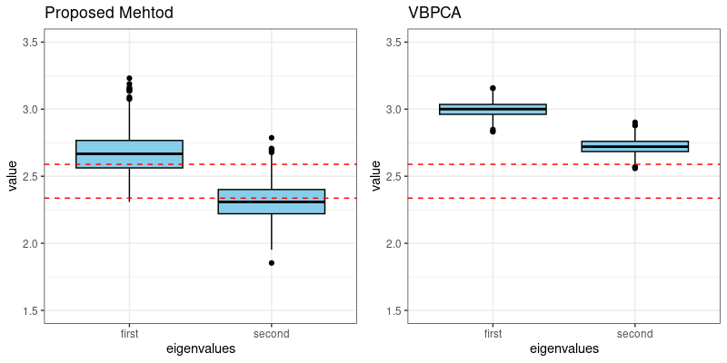
Figure 1: Boxplots of posterior samples for the two leading eigenvalues from the proposed method (left) and VBPCA (right). The red dashed lines represent the two leading eigenvalues for the sample covariance (SCOV).

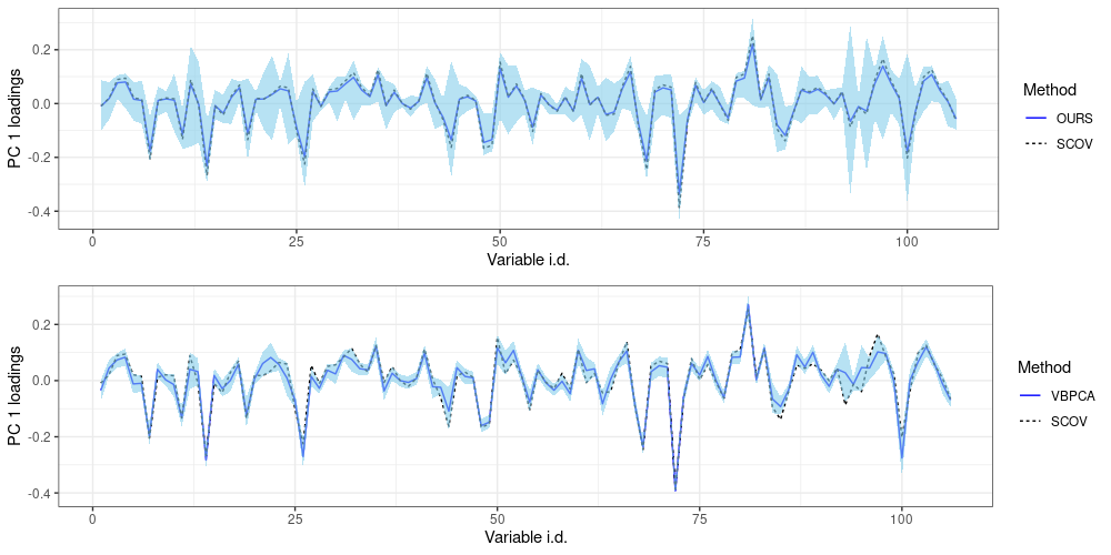
Figure 2: Comparison of PCA loading plots for the first leading component: the proposed method (top) and VBPCA (bottom). The shaded regions indicate the 95% credible intervals from the posterior distribution, providing uncertainty estimates for the loadings. The dashed lines represent the loadings derived from the sample covariance (SCOV).

We use the eigenvalue ratio estimator from Ahn and Horenstein (2013) to determine the optimal number of factors, which results in $\displaystyle K=2$. All methods are then fitted using these two factors, and the results are compared in terms of the eigenvalues and corresponding eigenvectors of each estimator, as presented in Figure 1 and 2. Figure 1 shows that the proposed method provides eigenvalue estimates close to those of SCOV with a wider credible interval compared to VBPCA. In contrast, VBPCA tends to overestimate the first and second eigenvalues compared to both SCOV and the proposed method. As depicted in Figure 2, for eigenvector estimation, the proposed method and VBPCA show distinct patterns in the first PC loadings. The proposed method closely aligns with the sample covariance loadings, and its credible intervals are comparatively wider compared to VBPCA, reflecting higher uncertainty. Especially, the variability in the first PC loadings increases between the 85th and 100th variables. On the other hand, VBPCA produces point estimates that deviate slightly from SCOV. These results indicate that the proposed method provides reasonable loading estimates with more conservative uncertainty compared to VBPCA.

5 Concluding remarks

We proposed Bayesian methods for estimating the spiked eigenstructure of high-dimensional covariances in the context of Bayesian principal component analysis. The proposed methods offer advantages in quantifying uncertainties in estimates compared to existing approaches and are theoretically justified in the high-dimensional setting through posterior contraction rates. We have shown that the posterior distribution of the spiked eigenvector is minimax optimal in the single spiked covariance model. Future work aims to extend the minimax analysis to multi-spiked covariance models.

6 Proof

In this section, we prove one of the main theorems, Theorem 3.3. The proof of other theorems, corollaries, propositions and additional lemmas are given in the Appendix section. For the proof of Theorem 3.3, we provide Lemmas 6.1-6.5, the proofs of which are given in the Appendix F.

Lemma 6.1.

Let $\displaystyle\bm{\Sigma}$ and $\displaystyle\bm{\Sigma}_{0}$ denote $\displaystyle p\times p$ positive-definite matrices. Let $\displaystyle\lambda_{k}$ and $\displaystyle\lambda_{0,k}$ denote the $\displaystyle k$th eigenvalues of $\displaystyle\bm{\Sigma}$ and $\displaystyle\bm{\Sigma}_{0}$, respectively, and let $\displaystyle\bm{u}_{k}$ and $\displaystyle\bm{u}_{0,k}$ denote the corresponding eigenvectors. If $\displaystyle\lambda_{0,k}||\bm{\Lambda}_{0,-k}^{-1/2}(\bm{U}_{0,-k}^{T}\bm{\Omega}\bm{U}_{0,-k}-\lambda_{k}\bm{\Lambda}_{0,-k}^{-1})^{-1}\bm{U}_{0,-k}^{T}\bm{\Omega}\bm{u}_{0,k}||_{2}^{2}<1$, then

$$\displaystyle(\bm{u}_{k}^{T}\bm{u}_{0,k})^{2}=\frac{1}{1+||\sqrt{\lambda_{0,k}}\bm{\Lambda}_{0,-k}^{-1/2}(\bm{U}_{0,-k}^{T}\bm{\Omega}\bm{U}_{0,-k}-\lambda_{k}\bm{\Lambda}_{0,-k}^{-1})^{-1}\bm{U}_{0,-k}^{T}\bm{\Omega}\bm{u}_{0,k}||_{2}^{2}}$$

where $\displaystyle\bm{\Omega}=\bm{\Sigma}_{0}^{-1/2}\bm{\Sigma}\bm{\Sigma}_{0}^{-1/2}$, $\displaystyle\bm{U}_{0,-k}=[\bm{u}_{0,1},\ldots,\bm{u}_{0,k-1},\bm{u}_{0,k+1},\ldots,\bm{u}_{0,p}]\in\mathbb{R}^{p\times(p-1)}$ and $\displaystyle\bm{\Lambda}_{0,-k}=\textup{diag}(\lambda_{0,1},\ldots,\lambda_{0,k-1},\lambda_{0,k+1},\ldots,\lambda_{0,p})$.

Lemma 6.2.

Let

$$\displaystyle\bm{A}=\begin{pmatrix}\bm{A}_{11}&\bm{A}_{12}\\ \bm{A}_{21}&\bm{A}_{22}\end{pmatrix}\in\mathbb{R}^{p\times p},$$

where $\displaystyle\bm{A}_{11}\in\mathbb{R}_{p_{1}\times p_{1}}$ and $\displaystyle\bm{A}_{22}\in\mathbb{R}_{p_{2}\times p_{2}}$. Then,

$$\displaystyle||\bm{A}_{12}||_{2} \displaystyle\leq \displaystyle||\bm{A}||_{2}.$$

Lemma 6.3.

Let $\displaystyle\bm{\Omega}\in\mathcal{C}_{p}$, and let $\displaystyle\bm{\Gamma}=[\bm{\Gamma}_{1},\bm{\Gamma}_{2}]\in\mathbb{R}^{p\times q}$ be an orthogonal matrix with $\displaystyle\bm{\Gamma}_{1}\in\mathbb{R}^{p\times q_{1}}$ and $\displaystyle\bm{\Gamma}_{2}\in\mathbb{R}^{p\times q_{2}}$.

$$\displaystyle||\bm{\Gamma}_{1}^{T}\bm{\Omega}\bm{\Gamma}_{2}||_{2}\leq||\bm{\Gamma}^{T}(\bm{\Omega}-\bm{I}_{p})\bm{\Gamma}||_{2}.$$

Lemma 6.4.

Suppose $\displaystyle\max\Big{\{}\frac{\lambda_{0,k}}{\lambda_{0,l}},\frac{\lambda_{0,l}}{\lambda_{0,k}}\Big{\}}>c>1$. If $\displaystyle|\frac{\lambda_{k}}{\lambda_{0,k}}-1|\leq\delta:=\delta(c)=(1-1/c)/4\wedge(1-1/c)/(2(2-1/c))\wedge 1/2$, then

$$\displaystyle|\frac{\lambda_{k}}{\lambda_{0,l}}-1| \displaystyle\geq \displaystyle(1-1/c)/2,$$

$$\displaystyle\frac{\sqrt{\lambda_{k}\lambda_{0,l}}}{|\lambda_{k}-\lambda_{0,l}|} \displaystyle\leq \displaystyle\frac{2\sqrt{2}}{1-1/c}\min\Big{\{}\sqrt{\frac{\lambda_{0,l}}{\lambda_{0,k}}},\sqrt{\frac{\lambda_{0,k}}{\lambda_{0,l}}}\Big{\}}.$$

Lemma 6.5.

Let $\displaystyle\bm{A},\bm{B}\in\mathcal{C}_{p}$. If $\displaystyle\lambda_{\min}(\bm{A})>||\bm{B}||_{2}$, then

$$\displaystyle||(\bm{A}-\bm{B})^{-1}||_{2}\leq\frac{1}{\lambda_{\min}(\bm{A})-||\bm{B}||_{2}}.$$

Using these lemmas, we prove Theorem 3.3.

Proof of Theorem 3.3.

We show $\displaystyle 1-(\bm{u}_{l}^{T}\bm{u}_{0,l})^{2}\leq Ct$ when $\displaystyle|\frac{\lambda_{l}}{\lambda_{0,l}}-1|\leq\delta_{1}$, $\displaystyle||\bm{\Gamma}^{T}\bm{\Omega}\bm{\Gamma}-\bm{I}_{K}||_{2}\leq\frac{\sqrt{t}}{\sqrt{B_{k}}}\wedge\delta_{2}$ and $\displaystyle\frac{\sqrt{\lambda_{0,K+1}}||\bm{\Gamma}_{\perp}^{T}\bm{\Omega}\bm{\Gamma}_{\perp}||^{1/2}}{\sqrt{\lambda_{0,l}}}\leq\sqrt{t}$ (or $\displaystyle\frac{\sqrt{\lambda_{0,K+1}}}{\sqrt{\lambda_{0,l}}}||\bm{\Omega}-\bm{I}_{p}||_{2}\leq\sqrt{t}$), where $\displaystyle\bm{\Omega}=\bm{\Sigma}_{0}^{-1/2}\bm{\Sigma}\bm{\Sigma}_{0}^{-1/2}$, $\displaystyle t\leq\Big{(}\frac{\lambda_{0,K+1}}{\lambda_{0,l}}\Big{)}^{1/4}(1-\delta_{1})\wedge(d^{-1/8}-d^{1/2})^{2}\wedge\frac{\delta_{2}}{2c_{l}(1+\delta_{2})}$, and $\displaystyle C$ is some positive constant dependent on $\displaystyle c$ and $\displaystyle d$.

We obtain $\displaystyle\lambda_{0,l}\leq\lambda_{l}/(1-\delta_{1})\leq 2\lambda_{l}$ from $\displaystyle|\frac{\lambda_{l}}{\lambda_{0,l}}-1|\leq\delta_{1}$ by setting $\displaystyle\delta_{1}<1/2$. Then, by Lemma 6.1, we have

$$\displaystyle 1-(\bm{u}_{l}^{T}\bm{u}_{0,l})^{2} \displaystyle\leq \displaystyle||\sqrt{\lambda_{0,l}}\bm{\Lambda}_{0,-l}^{-1/2}(\bm{U}_{0,-l}^{T}\bm{\Omega}\bm{U}_{0,-l}-\lambda_{l}\bm{\Lambda}_{0,-l}^{-1})^{-1}\bm{U}_{0,-l}^{T}\bm{\Omega}\bm{u}_{0,l}||_{2}^{2}$$

$$\displaystyle\leq \displaystyle 2||\sqrt{\lambda_{l}}\bm{\Lambda}_{0,-l}^{-1/2}(\bm{U}_{0,-l}^{T}\bm{\Omega}\bm{U}_{0,-l}-\lambda_{k}\bm{\Lambda}_{0,-l}^{-1})^{-1}\bm{U}_{0,-l}^{T}\bm{\Omega}\bm{u}_{0,l}||_{2}^{2},$$

where $\displaystyle\bm{\Lambda}_{0,-l}=\textup{diag}(\bm{\Lambda}_{(1)},\bm{\Lambda}_{(2)})$ and $\displaystyle\bm{U}_{0,-l}=[\bm{U}_{(1)},\bm{U}_{(2)}]$.

In this expression, $\displaystyle\bm{\Lambda}_{(1)}=\textup{diag}(\lambda_{0,1},\ldots,\lambda_{0,l-1},\lambda_{0,l+1},\ldots,\lambda_{0,K})\in\mathcal{C}_{K-1}$ and $\displaystyle\bm{\Lambda}_{(2)}=\textup{diag}(\lambda_{0,K+1},\ldots,\lambda_{0,p})\in\mathcal{C}_{p-K}$ are diagonal matrices. Similarly, $\displaystyle\bm{U}_{(1)}=[\bm{u}_{0,1},\ldots,\bm{u}_{0,l-1},\bm{u}_{0,l+1},\ldots,\bm{u}_{0,K}]\in\mathbb{R}^{p\times(K-1)}$ and $\displaystyle\bm{U}_{(2)}=\bm{\Gamma}_{\perp}=[\bm{u}_{0,K+1},\ldots,\bm{u}_{0,p}]\in\mathbb{R}^{p\times(p-K)}$ are orthogonal matrices. Since $\displaystyle\bm{\Gamma}$ consists of the column vectors of $\displaystyle\bm{U}_{(1)}$ and $\displaystyle\bm{u}_{0,l}$, by Lemma 6.3,

$$\displaystyle||\bm{U}_{(1)}^{T}\bm{\Omega}\bm{U}_{(1)}-\bm{I}_{K-1}||_{2} \displaystyle\leq \displaystyle||\bm{\Gamma}^{T}\bm{\Omega}\bm{\Gamma}-\bm{I}_{K}||_{2}\leq\sqrt{t}/\sqrt{B}\wedge\delta_{2}$$

$$\displaystyle||\bm{U}_{(1)}^{T}\bm{\Omega}\bm{u}_{0,l}||_{2} \displaystyle\leq \displaystyle||\bm{\Gamma}^{T}\bm{\Omega}\bm{\Gamma}-\bm{I}_{K}||_{2}\leq\sqrt{t}/\sqrt{B}\wedge\delta_{2}.$$

Under condition $\displaystyle\frac{\sqrt{\lambda_{0,K+1}}||\bm{\Gamma}_{\perp}^{T}\bm{\Omega}\bm{\Gamma}_{\perp}||_{2}^{1/2}}{\sqrt{\lambda_{0,l}}}\leq\sqrt{t}$, we have

$$\displaystyle\frac{\lambda_{0,K+1}}{\lambda_{l}}||\bm{U}_{(2)}^{T}\bm{\Omega}\bm{U}_{(2)}||_{2} \displaystyle\leq \displaystyle\frac{1}{1-\delta_{1}}\frac{\lambda_{0,K+1}}{\lambda_{0,l}}||\bm{U}_{(2)}^{T}\bm{\Omega}\bm{U}_{(2)}||_{2}$$

$$\displaystyle= \displaystyle\frac{1}{1-\delta_{1}}\frac{\lambda_{0,K+1}}{\lambda_{0,l}}||\bm{\Gamma}_{\perp}^{T}\bm{\Omega}\bm{\Gamma}_{\perp}||_{2},$$

$$\displaystyle\leq \displaystyle\frac{t}{1-\delta_{1}}$$

$$\displaystyle\leq \displaystyle\frac{\delta}{1-\delta_{1}},$$

where the last inequality is satisfied since $\displaystyle t\leq\delta$. Under condition $\displaystyle\frac{\sqrt{\lambda_{0,K+1}}}{\sqrt{\lambda_{0,l}}}||\bm{\Omega}-\bm{I}_{p}||_{2}\leq\sqrt{t}$,

$$\displaystyle\frac{\lambda_{0,K+1}}{\lambda_{l}}||\bm{U}_{(2)}^{T}\bm{\Omega}\bm{U}_{(2)}||_{2} \displaystyle\leq \displaystyle\frac{1}{1-\delta_{1}}\frac{\lambda_{0,K+1}}{\lambda_{0,l}}||\bm{U}_{(2)}^{T}\bm{\Omega}\bm{U}_{(2)}||_{2}$$

$$\displaystyle\leq \displaystyle\frac{1}{1-\delta_{1}}\frac{\lambda_{0,K+1}}{\lambda_{0,l}}(1+||\bm{\Omega}-\bm{I}_{p}||_{2})$$

$$\displaystyle\leq \displaystyle\frac{1}{1-\delta_{1}}(\frac{\lambda_{0,K+1}}{\lambda_{0,l}}+\sqrt{\frac{\lambda_{0,K+1}}{\lambda_{0,l}}}\sqrt{t})$$

$$\displaystyle\leq \displaystyle\Big{(}\frac{\lambda_{0,K+1}}{\lambda_{0,l}}\Big{)}^{1/4},$$

where the last inequality is satisfied by the following. Let $\displaystyle x=\frac{\lambda_{0,K+1}}{\lambda_{0,l}}$. We have $\displaystyle x\leq d<1$ and set $\displaystyle\delta_{1}$ and $\displaystyle\delta$ to satisfy $\displaystyle\delta_{1}\leq 1-d^{1/8}\leq 1-x^{1/8}$ and $\displaystyle\sqrt{t}\leq\sqrt{\delta}\leq d^{-1/8}-d^{1/2}\leq x^{-1/8}-x^{1/2}$. Then,

$$\displaystyle\frac{1}{1-\delta_{1}}(\frac{\lambda_{0,K+1}}{\lambda_{0,l}}+\sqrt{\frac{\lambda_{0,K+1}}{\lambda_{0,l}}}\sqrt{t}) \displaystyle= \displaystyle\sqrt{x}\frac{\sqrt{x}+\sqrt{t}}{1-\delta_{1}}$$

$$\displaystyle\leq \displaystyle\sqrt{x}\frac{x^{-1/8}}{x^{1/8}}$$

$$\displaystyle= \displaystyle x^{1/4}$$

$$\displaystyle= \displaystyle\Big{(}\frac{\lambda_{0,K+1}}{\lambda_{0,l}}\Big{)}^{1/4}.$$

Thus,

$$\displaystyle\frac{\lambda_{0,K+1}}{\lambda_{l}}||\bm{U}_{(2)}^{T}\bm{\Omega}\bm{U}_{(2)}||_{2} \displaystyle\leq \displaystyle\Big{(}\frac{\lambda_{0,K+1}}{\lambda_{0,l}}\Big{)}^{1/4}\vee\frac{\delta}{1-\delta_{1}}$$ (9)

$$\displaystyle\leq \displaystyle\Big{(}\frac{\lambda_{0,K+1}}{\lambda_{0,l}}\Big{)}^{1/4}\vee\frac{1}{2},$$

by setting $\displaystyle\delta$ to satisfy $\displaystyle\frac{\delta}{1-\delta_{1}}\leq\frac{1}{2}$.

Under condition $\displaystyle\frac{\sqrt{\lambda_{0,K+1}}||\bm{\Gamma}_{\perp}^{T}\bm{\Omega}\bm{\Gamma}_{\perp}||_{2}^{1/2}}{\sqrt{\lambda_{0,l}}}\leq\sqrt{t}$, we have

$$\displaystyle\sqrt{\frac{\lambda_{0,K+1}}{\lambda_{l}}}||\bm{U}_{(1)}^{T}\bm{\Omega}\bm{U}_{(2)}||_{2} \displaystyle\leq \displaystyle\sqrt{\frac{2\lambda_{0,K+1}}{\lambda_{0,l}}}||\bm{U}_{(1)}^{T}\bm{\Omega}^{1/2}||_{2}||\bm{\Omega}^{1/2}\bm{U}_{(2)}||_{2}$$

$$\displaystyle{\color[rgb]{.75,0,.25}=} \displaystyle||\bm{U}_{(1)}^{T}\bm{\Omega}\bm{U}_{(1)}||_{2}^{1/2}\Big{(}\frac{2\lambda_{0,K+1}}{\lambda_{0,l}}||\bm{U}_{(2)}^{T}\bm{\Omega}\bm{U}_{(2)}||_{2}\Big{)}^{1/2}$$

$$\displaystyle\leq \displaystyle||\bm{\Gamma}^{T}\bm{\Omega}\bm{\Gamma}||_{2}^{1/2}\Big{(}\frac{2\lambda_{0,K+1}}{\lambda_{0,l}}||\bm{\Gamma}_{\perp}^{T}\bm{\Omega}\bm{\Gamma}_{\perp}||_{2}\Big{)}^{1/2}$$

$$\displaystyle\leq \displaystyle(1+||\bm{I}_{K}-\bm{\Gamma}^{T}\bm{\Omega}\bm{\Gamma}||_{2})^{1/2}\sqrt{2t}$$

$$\displaystyle\leq \displaystyle\sqrt{2(1+\delta_{2})t},$$

and under condition $\displaystyle\frac{\sqrt{\lambda_{0,K+1}}}{\sqrt{\lambda_{0,l}}}||\bm{\Omega}-\bm{I}_{p}||_{2}\leq\sqrt{t}$,

$$\displaystyle\sqrt{\frac{\lambda_{0,K+1}}{\lambda_{l}}}||\bm{U}_{(1)}^{T}\bm{\Omega}\bm{U}_{(2)}||_{2} \displaystyle\leq \displaystyle\sqrt{\frac{\lambda_{0,K+1}}{\lambda_{l}}}||\bm{\Omega}-\bm{I}_{p}||_{2}$$

$$\displaystyle\leq \displaystyle\sqrt{t}$$

$$\displaystyle\leq \displaystyle\sqrt{2(1+\delta_{2})t},$$

where the first inequality is satisfied by Lemma 6.3. Likewise, we obtain

$$\displaystyle\sqrt{\frac{\lambda_{0,K+1}}{\lambda_{l}}}||\bm{U}_{(2)}^{T}\bm{\Omega}\bm{u}_{0,l}||_{2}\leq\sqrt{2(1+\delta_{2})t}.$$

We expand $\displaystyle(\bm{U}_{0,-l}^{T}\bm{\Omega}\bm{U}_{0,-l}-\lambda_{l}\bm{\Lambda}_{0,-l}^{-1})^{-1}$ as

$$\displaystyle(\bm{U}_{0,-l}^{T}\bm{\Omega}\bm{U}_{0,-l}-\lambda_{l}\bm{\Lambda}_{0,-l}^{-1})^{-1}$$

$$\displaystyle= \displaystyle\begin{pmatrix}\bm{U}_{(1)}^{T}\bm{\Omega}\bm{U}_{(1)}-\lambda_{l}\bm{\Lambda}_{(1)}^{-1}&\bm{U}_{(1)}^{T}\bm{\Omega}\bm{U}_{(2)}\\ (\bm{U}_{(1)}^{T}\bm{\Omega}\bm{U}_{(2)})^{T}&\bm{U}_{(2)}^{T}\bm{\Omega}\bm{U}_{(2)}-\lambda_{l}\bm{\Lambda}_{(2)}^{-1}\end{pmatrix}^{-1}$$

$$\displaystyle= \displaystyle\begin{pmatrix}\bm{A}&\bm{B}\\ \bm{B}^{T}&\bm{C}\end{pmatrix}^{-1}$$

$$\displaystyle= \displaystyle\begin{pmatrix}\bm{B}_{11}&\bm{B}_{12}\\ \bm{B}_{12}^{T}&\bm{B}_{22}\end{pmatrix},$$

where $\displaystyle\bm{B}_{11}=(\bm{A}-\bm{B}\bm{C}^{-1}\bm{B}^{T})^{-1}$, $\displaystyle\bm{B}_{12}=-(\bm{A}-\bm{B}\bm{C}^{-1}\bm{B}^{T})^{-1}\bm{B}\bm{C}^{-1}=-\bm{B}_{11}\bm{B}\bm{C}^{-1}$ and $\displaystyle\bm{B}_{22}=\bm{C}^{-1}+\bm{C}^{-1}\bm{B}^{T}(\bm{A}-\bm{B}\bm{C}^{-1}\bm{B}^{T})^{-1}\bm{B}\bm{C}^{-1}$. Then,

$$\displaystyle||\sqrt{\lambda_{l}}\bm{\Lambda}_{0,-l}^{-1/2}(\bm{U}_{-l}^{T}\bm{\Omega}\bm{U}_{-l}-\lambda_{l}\bm{\Lambda}_{0,-l}^{-1})^{-1}\bm{U}_{-l}^{T}\bm{\Omega}\bm{u}_{0,l}||_{2}$$

$$\displaystyle= \displaystyle||\begin{pmatrix}\sqrt{\lambda_{l}}\bm{\Lambda}_{(1)}^{-1/2}\bm{B}_{11}\bm{U}_{(1)}^{T}\bm{\Omega}\bm{u}_{0,l}+\sqrt{\lambda_{l}}\bm{\Lambda}_{(1)}^{-1/2}\bm{B}_{12}\bm{U}_{(2)}^{T}\bm{\Omega}\bm{u}_{0,l}\\ \sqrt{\lambda_{l}}\bm{\Lambda}_{(2)}^{-1/2}\bm{B}_{12}^{T}\bm{U}_{(1)}^{T}\bm{\Omega}\bm{u}_{0,l}+\sqrt{\lambda_{l}}\bm{\Lambda}_{(2)}^{-1/2}\bm{B}_{22}\bm{U}_{(2)}^{T}\bm{\Omega}\bm{u}_{0,l}\end{pmatrix}||_{2}$$

$$\displaystyle\leq \displaystyle||\sqrt{\lambda_{l}}\bm{\Lambda}_{(1)}^{-1/2}\bm{B}_{11}||_{2}||\bm{U}_{(1)}^{T}\bm{\Omega}\bm{u}_{0,l}||_{2}+||\sqrt{\lambda_{l}}\bm{\Lambda}_{(1)}^{-1/2}\bm{B}_{12}||_{2}||\bm{U}_{(2)}^{T}\bm{\Omega}\bm{u}_{0,l}||_{2}$$

$$\displaystyle+||\sqrt{\lambda_{l}}\bm{\Lambda}_{(2)}^{-1/2}\bm{B}_{12}^{T}||_{2}||\bm{U}_{(1)}^{T}\bm{\Omega}\bm{u}_{0,l}||_{2}+||\sqrt{\lambda_{l}}\bm{\Lambda}_{(2)}^{-1/2}\bm{B}_{22}||_{2}||\bm{U}_{(2)}^{T}\bm{\Omega}\bm{u}_{0,l}||_{2}.$$

We have

$$\displaystyle\bm{B}_{11} \displaystyle= \displaystyle(\bm{U}_{(1)}^{T}\bm{\Omega}\bm{U}_{(1)}-\bm{I}_{K-1}+\bm{I}_{K-1}-\lambda_{l}\bm{\Lambda}_{(1)}^{-1}-\bm{B}\bm{C}^{-1}\bm{B}^{T})^{-1}$$

$$\displaystyle= \displaystyle\bm{D}_{1}(\bm{I}_{K-1}+(\bm{U}_{(1)}^{T}\bm{\Omega}\bm{U}_{(1)}-\bm{I}_{K-1}-\bm{B}\bm{C}^{-1}\bm{B}^{T})\bm{D}_{1})^{-1},$$

where $\displaystyle\bm{D}_{1}=(\bm{I}_{K-1}-\lambda_{l}\bm{\Lambda}_{(1)}^{-1})^{-1}=\textup{diag}(\frac{\lambda_{0,1}}{\lambda_{0,1}-\lambda_{l}},\ldots,\frac{\lambda_{0,l-1}}{\lambda_{0,l-1}-\lambda_{l}},\frac{\lambda_{0,l+1}}{\lambda_{0,l+1}-\lambda_{l}},\ldots,\frac{\lambda_{0,K}}{\lambda_{0,K}-\lambda_{l}})$ and

$$\displaystyle||\bm{D}_{1}||_{2}\leq 2/(1-1/c)=1/(4\delta_{2})$$ (10)

by Lemma 6.4 where $\displaystyle\delta_{2}$ is set to satisfy $\displaystyle 2/(1-1/c)=1/(4\delta_{2})$.

Let $\displaystyle c_{l}=\frac{1}{1-(\lambda_{0,K+1}/\lambda_{0,l})^{1/4}\vee\frac{1}{2}}$. We have

$$\displaystyle\lambda_{l}||\bm{C}^{-1}||_{2}/\lambda_{0,K+1} \displaystyle\leq \displaystyle\frac{\lambda_{l}}{\lambda_{0,K+1}\{\lambda_{l}/||\bm{\Lambda}_{(2)}||_{2}-||\bm{U}_{(2)}^{T}\bm{\Omega}\bm{U}_{(2)}||_{2}\}}$$

$$\displaystyle= \displaystyle\frac{1}{1-\lambda_{0,K+1}||\bm{U}_{(2)}^{T}\bm{\Omega}\bm{U}_{(2)}||_{2}/\lambda_{l}}$$

$$\displaystyle\leq \displaystyle\frac{1}{1-(\lambda_{0,K+1}/\lambda_{0,l})^{1/4}}$$

$$\displaystyle\leq \displaystyle c_{l},$$

where the first inequality is satisfied by Lemma 6.5. To apply Lemma 6.5, we show $\displaystyle\lambda_{l}/||\bm{\Lambda}_{(2)}||_{2}>||\bm{U}_{(2)}^{T}\bm{\Omega}\bm{U}_{(2)}||_{2}$. Since $\displaystyle\lambda_{0,K+1}=||\bm{\Lambda}_{(2)}||_{2}$, it suffices to show $\displaystyle 1>\lambda_{0,K+1}||\bm{U}_{(2)}^{T}\bm{\Omega}\bm{U}_{(2)}||_{2}/\lambda_{l}$, which is shown by (9). We also have

$$\displaystyle||\bm{U}_{(1)}^{T}\bm{\Omega}\bm{U}_{(1)}-\bm{I}_{K-1}-\bm{B}\bm{C}^{-1}\bm{B}^{T}|| \displaystyle\leq \displaystyle||\bm{U}_{(1)}^{T}\bm{\Omega}\bm{U}_{(1)}-\bm{I}_{K-1}||+||\bm{B}||_{2}^{2}||\bm{C}^{-1}||_{2}$$ (11)

$$\displaystyle\leq \displaystyle||\bm{U}_{(1)}^{T}\bm{\Omega}\bm{U}_{(1)}-\bm{I}_{K-1}||+c_{l}||\bm{U}_{(1)}^{T}\bm{\Omega}\bm{U}_{(2)}||^{2}\lambda_{0,K+1}/\lambda_{l}$$

$$\displaystyle\leq \displaystyle\delta_{2}+2c_{l}(1+\delta_{2})t$$

$$\displaystyle\leq \displaystyle 2\delta_{2},$$

where the last inequality is satisfied by setting $\displaystyle\delta$ to satisfy $\displaystyle t\leq\delta\leq\Big{(}\frac{\delta_{2}}{2c_{l}(1+\delta_{2})}\Big{)}$. Thus,

$$\displaystyle||\sqrt{\lambda_{l}}\bm{\Lambda}_{(1)}^{-1/2}\bm{B}_{11}||_{2}$$

$$\displaystyle\leq \displaystyle||\sqrt{\lambda_{l}}\bm{\Lambda}_{(1)}^{-1/2}\bm{D}_{1}||_{2}||(\bm{I}_{K-1}+(\bm{U}_{(1)}^{T}\bm{\Omega}\bm{U}_{(1)}-\bm{I}_{K-1}-\bm{B}\bm{C}^{-1}\bm{B}^{T})\bm{D}_{1})^{-1}||_{2}$$

$$\displaystyle\leq \displaystyle\frac{||\sqrt{\lambda_{l}}\bm{\Lambda}_{(1)}^{-1/2}\bm{D}_{1}||_{2}}{1-||\bm{D}_{1}||_{2}||\bm{U}_{(1)}^{T}\bm{\Omega}\bm{U}_{(1)}-\bm{I}_{K-1}-\bm{B}\bm{C}^{-1}\bm{B}^{T}||_{2}}$$

$$\displaystyle\leq \displaystyle 2||\sqrt{\lambda_{l}}\bm{\Lambda}_{(1)}^{-1/2}\bm{D}_{1}||_{2},$$

where the last inequality is satisfied by (10) and (11).

Next, we have

$$\displaystyle||\sqrt{\lambda_{l}}\bm{\Lambda}_{(1)}^{-1/2}\bm{B}_{12}||_{2} \displaystyle\leq \displaystyle||\sqrt{\lambda_{l}}\bm{\Lambda}_{(1)}^{-1/2}\bm{B}_{11}||_{2}||\bm{U}_{(1)}^{T}\bm{\Omega}\bm{U}_{(2)}||_{2}||\bm{C}^{-1}||_{2}$$

$$\displaystyle= \displaystyle||\sqrt{\lambda_{l}}\bm{\Lambda}_{(1)}^{-1/2}\bm{B}_{11}||_{2}\lambda_{0,K+1}||\bm{U}_{(1)}^{T}\bm{\Omega}\bm{U}_{(2)}||_{2}/\lambda_{l}(\lambda_{l}||\bm{C}^{-1}||_{2}/\lambda_{0,K+1})$$

$$\displaystyle\leq \displaystyle 2||\sqrt{\lambda_{l}}\bm{\Lambda}_{(1)}^{-1/2}\bm{D}_{1}||_{2}\frac{\sqrt{\lambda_{0,K+1}}}{\sqrt{\lambda_{l}}}\sqrt{2(1+\delta_{2})t}c_{l}$$

$$\displaystyle= \displaystyle 2c_{l}\sqrt{2(1+\delta_{2})t}||\sqrt{\lambda_{l}}\bm{\Lambda}_{(1)}^{-1/2}\bm{D}_{1}||_{2}\frac{\sqrt{\lambda_{0,K+1}}}{\sqrt{\lambda_{l}}},$$

and

$$\displaystyle||\sqrt{\lambda_{l}}\bm{\Lambda}_{(2)}^{-1/2}\bm{C}^{-1}||_{2} \displaystyle= \displaystyle||\sqrt{\lambda_{l}}\bm{\Lambda}_{(2)}^{-1/2}[\bm{U}_{(2)}^{T}\bm{\Omega}\bm{U}_{(2)}-\lambda_{l}\bm{\Lambda}_{(2)}^{-1}]^{-1}||_{2}$$

$$\displaystyle= \displaystyle||[\bm{U}_{(2)}^{T}\bm{\Omega}\bm{U}_{(2)}(\sqrt{\lambda_{l}}\bm{\Lambda}_{(2)}^{-1/2})^{-1}-\sqrt{\lambda_{l}}\bm{\Lambda}_{(2)}^{-1/2}]^{-1}||_{2}$$

$$\displaystyle\leq \displaystyle 1/[\lambda_{\min}(\sqrt{\lambda_{l}}\bm{\Lambda}_{(2)}^{-1/2})-||\bm{U}_{(2)}^{T}\bm{\Omega}\bm{U}_{(2)}(\sqrt{\lambda_{l}}\bm{\Lambda}_{(2)}^{-1/2})^{-1}||_{2}]$$

$$\displaystyle= \displaystyle 1/[\sqrt{\lambda_{l}/||\bm{\Lambda}_{(2)}||_{2}}-||\bm{U}_{(2)}^{T}\bm{\Omega}\bm{U}_{(2)}(\sqrt{\lambda_{l}}\bm{\Lambda}_{(2)}^{-1/2})^{-1}||_{2}]$$

$$\displaystyle\leq \displaystyle 1/[\sqrt{\lambda_{l}/||\bm{\Lambda}_{(2)}||_{2}}-\lambda_{l}^{-1/2}||\bm{U}_{(2)}^{T}\bm{\Omega}\bm{U}_{(2)}||_{2}||\bm{\Lambda}_{(2)}||_{2}^{1/2}]$$

$$\displaystyle= \displaystyle\sqrt{\frac{\lambda_{0,K+1}}{\lambda_{l}}}\frac{1}{1-||\bm{U}_{(2)}^{T}\bm{\Omega}\bm{U}_{(2)}||_{2}\lambda_{0,K+1}/\lambda_{l}}$$

$$\displaystyle\leq \displaystyle c_{l}\sqrt{\frac{\lambda_{0,K+1}}{\lambda_{l}}},$$

where the first inequality is satisfied by Lemma 6.5. To apply Lemma 6.5, we have to show $\displaystyle\lambda_{\min}(\sqrt{\lambda_{l}}\bm{\Lambda}_{(2)}^{-1/2})>||\bm{U}_{(2)}^{T}\bm{\Omega}\bm{U}_{(2)}(\sqrt{\lambda_{l}}\bm{\Lambda}_{(2)}^{-1/2})^{-1}||_{2}$. Since

$$||\bm{U}_{(2)}^{T}\bm{\Omega}\bm{U}_{(2)}(\sqrt{\lambda_{l}}\bm{\Lambda}_{(2)}^{-1/2})^{-1}||_{2}\leq\lambda_{l}^{-1/2}||\bm{U}_{(2)}^{T}\bm{\Omega}\bm{U}_{(2)}||_{2}||\bm{\Lambda}_{(2)}||_{2}^{1/2},$$

it suffices to show $\displaystyle\sqrt{\lambda_{l}/||\bm{\Lambda}_{(2)}||_{2}}>\lambda_{l}^{-1/2}||\bm{U}_{(2)}^{T}\bm{\Omega}\bm{U}_{(2)}||_{2}||\bm{\Lambda}_{(2)}||_{2}^{1/2}$, equivalently $\displaystyle 1>||\bm{U}_{(2)}^{T}\bm{\Omega}\bm{U}_{(2)}||_{2}\lambda_{0,K+1}/\lambda_{l}$, which is shown by (9).

We have

$$\displaystyle||\bm{B}_{11}||_{2}$$

$$\displaystyle\leq \displaystyle||\bm{D}_{1}||_{2}||(\bm{I}_{K-1}+(\bm{U}_{(1)}^{T}\bm{\Omega}\bm{U}_{(1)}-\bm{I}_{K-1}-\bm{B}\bm{C}^{-1}\bm{B}^{T})\bm{D}_{1})^{-1}||_{2}$$

$$\displaystyle\leq \displaystyle\frac{||\bm{D}_{1}||_{2}}{1-||\bm{D}_{1}||_{2}||\bm{U}_{(1)}^{T}\bm{\Omega}\bm{U}_{(1)}-\bm{I}_{K-1}-\bm{B}\bm{C}^{-1}\bm{B}^{T}||_{2}}$$

$$\displaystyle\leq \displaystyle 2||\bm{D}_{1}||_{2}$$

$$\displaystyle\leq \displaystyle 1/(2\delta_{2}),$$

by (10) and (11). And, we have

$$\displaystyle||\sqrt{\lambda_{l}}\bm{\Lambda}_{(2)}^{-1/2}\bm{B}_{12}^{T}||_{2} \displaystyle\leq \displaystyle||\sqrt{\lambda_{l}}\bm{\Lambda}_{(2)}^{-1/2}\bm{C}^{-1}||_{2}||\bm{U}_{(1)}^{T}\bm{\Omega}\bm{U}_{(2)}||_{2}||\bm{B}_{11}||_{2}$$

$$\displaystyle\leq \displaystyle\frac{c_{l}}{2\delta_{2}}||\bm{U}_{(1)}^{T}\bm{\Omega}\bm{U}_{(2)}||_{2}\sqrt{\lambda_{0,K+1}}/\sqrt{\lambda_{l}}$$

$$\displaystyle\leq \displaystyle c_{l}\sqrt{2(1+\delta_{2})t}/(2\delta_{2}),$$

$$\displaystyle||\sqrt{\lambda_{l}}\bm{\Lambda}_{(2)}^{-1/2}\bm{B}_{22}||_{2} \displaystyle\leq \displaystyle||\sqrt{\lambda_{l}}\bm{\Lambda}_{(2)}^{-1/2}\bm{C}^{-1}||_{2}(1+||\bm{B}^{T}\bm{B}_{11}\bm{B}\bm{C}^{-1}||_{2})$$

$$\displaystyle\leq \displaystyle||\sqrt{\lambda_{l}}\bm{\Lambda}_{(2)}^{-1/2}\bm{C}^{-1}||_{2}(1+||\bm{B}_{11}||_{2}\frac{\lambda_{0,K+1}||\bm{U}_{(1)}^{T}\bm{\Omega}\bm{U}_{(2)}||_{2}^{2}}{\lambda_{l}}\frac{\lambda_{l}||\bm{C}^{-1}||_{2}}{\lambda_{0,K+1}})$$

$$\displaystyle\leq \displaystyle c_{l}\sqrt{\lambda_{0,K+1}/\lambda_{l}}(1+c_{l}(1+\delta_{2})t/\delta_{2}),$$

$$\displaystyle\sqrt{\lambda_{l}}\bm{\Lambda}_{(1)}^{-1/2}\bm{D}_{1} \displaystyle= \displaystyle\textup{diag}(\frac{\sqrt{\lambda_{l}\lambda_{0,1}}}{\lambda_{0,1}-\lambda_{l}},\ldots,\frac{\sqrt{\lambda_{l}\lambda_{0,l-1}}}{\lambda_{0,l-1}-\lambda_{l}},\frac{\sqrt{\lambda_{l}\lambda_{0,l+1}}}{\lambda_{0,l+1}-\lambda_{l}},\ldots,\frac{\sqrt{\lambda_{l}\lambda_{0,K}}}{\lambda_{0,K}-\lambda_{l}}),$$

and

$$\displaystyle||\sqrt{\lambda_{l}}\bm{\Lambda}_{(1)}^{-1/2}\bm{D}_{1}||_{2}\leq C_{1}\sqrt{B_{k}},$$

for some positive constant $\displaystyle C_{1}$ dependent on $\displaystyle c$ by Lemma 6.4.

Collecting the inequalities, we obtain

$$\displaystyle||\sqrt{\lambda_{l}}\bm{\Lambda}_{(1)}^{-1/2}\bm{B}_{11}\bm{U}_{(1)}^{T}\bm{\Omega}\bm{u}_{0,l}+\sqrt{\lambda_{l}}\bm{\Lambda}_{(1)}^{-1/2}\bm{B}_{12}\bm{U}_{(2)}^{T}\bm{\Omega}\bm{u}_{0,l}||_{2}$$

$$\displaystyle\leq \displaystyle||\sqrt{\lambda_{l}}\bm{\Lambda}_{(1)}^{-1/2}\bm{B}_{11}||_{2}||\bm{U}_{(1)}^{T}\bm{\Omega}\bm{u}_{0,l}||_{2}+||\sqrt{\lambda_{l}}\bm{\Lambda}_{(1)}^{-1/2}\bm{B}_{12}||_{2}||\bm{U}_{(2)}^{T}\bm{\Omega}\bm{u}_{0,l}||_{2}$$

$$\displaystyle\lesssim \displaystyle||\sqrt{\lambda_{l}}\bm{\Lambda}_{(1)}^{-1/2}\bm{D}_{1}||_{2}(\sqrt{t}/\sqrt{B_{k}}+\sqrt{t})$$

$$\displaystyle\lesssim \displaystyle\sqrt{t},$$

where the last inequality is satisfied since $\displaystyle B_{k}\leq 1$, and

$$\displaystyle||\sqrt{\lambda_{l}}\bm{\Lambda}_{(2)}^{-1/2}\bm{B}_{12}^{T}\bm{U}_{(1)}^{T}\bm{\Omega}\bm{u}_{0,l}+\sqrt{\lambda_{l}}\bm{\Lambda}_{(2)}^{-1/2}\bm{B}_{22}\bm{U}_{(2)}^{T}\bm{\Omega}\bm{u}_{0,l}||_{2}$$

$$\displaystyle\leq \displaystyle||\sqrt{\lambda_{l}}\bm{\Lambda}_{(2)}^{-1/2}\bm{B}_{12}^{T}||_{2}||\bm{U}_{(1)}^{T}\bm{\Omega}\bm{u}_{0,l}||_{2}+||\sqrt{\lambda_{l}}\bm{\Lambda}_{(2)}^{-1/2}\bm{B}_{22}||_{2}||\bm{U}_{(2)}^{T}\bm{\Omega}\bm{u}_{0,l}||_{2}$$

$$\displaystyle\leq \displaystyle||\sqrt{\lambda_{l}}\bm{\Lambda}_{(2)}^{-1/2}\bm{B}_{12}^{T}||_{2}||\bm{U}_{(1)}^{T}\bm{\Omega}\bm{u}_{0,l}||_{2}$$

$$\displaystyle+\sqrt{\frac{\lambda_{l}}{\lambda_{0,K+1}}}||\sqrt{\lambda_{l}}\bm{\Lambda}_{(2)}^{-1/2}\bm{B}_{22}||_{2}\sqrt{\frac{\lambda_{0,K+1}}{\lambda_{l}}}||\bm{U}_{(2)}^{T}\bm{\Omega}\bm{u}_{0,l}||_{2}$$

$$\displaystyle\lesssim \displaystyle c_{l}\sqrt{t}.$$

Then, we obtain

$$\displaystyle 1-(\bm{u}_{l}^{T}\bm{u}_{0,l})^{2}\leq Ct,$$

for some positive constant $\displaystyle C$ dependent on $\displaystyle c$ and $\displaystyle d$. Thus, we obtain

$$\displaystyle P(\sup_{l=1,\ldots,k}\{1-(\bm{u}_{l}^{T}\bm{u}_{0,l})^{2}\}>Ct) \displaystyle\leq \displaystyle P(||\bm{\Gamma}_{\perp}^{T}\bm{\Sigma}_{0}^{-1/2}\bm{\Sigma}\bm{\Sigma}_{0}^{-1/2}\bm{\Gamma}_{\perp}||_{2}^{1/2}\frac{\sqrt{\lambda_{0,K+1}}}{\sqrt{\lambda_{0,k}}}>\sqrt{t})$$

$$\displaystyle+P(||\bm{\Gamma}^{T}\bm{\Sigma}_{0}^{-1/2}\bm{\Sigma}\bm{\Sigma}_{0}^{-1/2}\bm{\Gamma}-\bm{I}_{K}||_{2}>\frac{\sqrt{t}}{\sqrt{B}}\wedge\delta_{2})$$

$$\displaystyle+P(\sup_{l=1,\ldots,k}|\frac{\lambda_{l}}{\lambda_{0,l}}-1|>\delta_{1}).$$

∎

Appendix A Concentration of eigenvalues under low-dimensional case

In this section, we provide Theorem A.1 for the eigenvalue concentration inequality when $\displaystyle p||\bm{\Sigma}_{0}^{-1/2}\bm{\Sigma}\bm{\Sigma}_{0}^{-1/2}-\bm{I}_{p}||_{2}$ is small enough. Theorem A.1 is used for the proof of Theorem 3.1.

Theorem A.1.

Let $\displaystyle\lambda_{1}\geq\ldots\geq\lambda_{p}>0$ be the eigenvalues of $\displaystyle\bm{\Sigma}$ and let $\displaystyle d_{1}\geq\ldots\geq d_{p}>0$ be the eigenvalues of $\displaystyle\bm{\Sigma}_{0}$ with $\displaystyle\min_{l=1,\ldots,p-1}\frac{d_{l}}{d_{l+1}}>c$ for some constant $\displaystyle c>1$. If $\displaystyle p||\bm{\Sigma}_{0}^{-1/2}\bm{\Sigma}\bm{\Sigma}_{0}^{-1/2}-\bm{I}_{p}||_{2}<\delta$ for some positive constant $\displaystyle\delta$ dependent on $\displaystyle c$, then

$$\displaystyle\sup_{k=1,\ldots,p}|\frac{\lambda_{k}}{d_{k}}-1|\leq Cp||\bm{\Sigma}_{0}^{-1/2}\bm{\Sigma}\bm{\Sigma}_{0}^{-1/2}-\bm{I}_{p}||_{2},$$

$$\displaystyle\sup_{k=1,\ldots,p}|\frac{\sqrt{\lambda_{k}}}{\sqrt{d_{k}}}-1|\leq Cp||\bm{\Sigma}_{0}^{-1/2}\bm{\Sigma}\bm{\Sigma}_{0}^{-1/2}-\bm{I}_{p}||_{2}.$$

for some positive constant $\displaystyle C$ dependent on $\displaystyle c$.

The proof of Theorem A.1 is given below with the following lemma.

Lemma A.2.

Suppose $\displaystyle d_{1}\geq d_{2}\geq\ldots\geq d_{p}\geq 0$, $\displaystyle\lambda>0$ and $\displaystyle 1\leq k\leq p$. If $\displaystyle\min_{l=1,\ldots,p-1}\frac{d_{l}}{d_{l+1}}>c$ and $\displaystyle|\lambda/d_{k}-1|<\frac{c-1}{2c}$ with $\displaystyle c>1$, then

$$\displaystyle\lambda/d_{j}-1 \displaystyle\geq \displaystyle\frac{c-1}{2},~\textup{when }j>k,$$

$$\displaystyle 1-\lambda/d_{j} \displaystyle\geq \displaystyle\frac{c-1}{c}\Big{(}1-\frac{1}{2c}\Big{)},~\textup{when }j<k.$$

Proof of Lemma A.2.

First, we consider $\displaystyle j>k$ which implies $\displaystyle d_{k}/d_{j}>c$. We have

$$\displaystyle\lambda/d_{j}-1 \displaystyle= \displaystyle\frac{d_{k}}{d_{j}}|\frac{\lambda}{d_{k}}|-1$$

$$\displaystyle\geq \displaystyle c(1-|\frac{\lambda}{d_{k}}-1|)-1$$

$$\displaystyle\geq \displaystyle c(1-\frac{c-1}{2c})-1$$

$$\displaystyle= \displaystyle\frac{c-1}{2}.$$

Next, we consider $\displaystyle j<k$ which implies $\displaystyle d_{j}/d_{k}>c$. We have

$$\displaystyle 1-\lambda/d_{j} \displaystyle= \displaystyle 1-\frac{\lambda}{d_{k}}\frac{d_{k}}{d_{j}}$$

$$\displaystyle\geq \displaystyle 1-\frac{1}{c}(1+|\frac{\lambda}{d_{k}}-1|)$$

$$\displaystyle= \displaystyle 1-\frac{1}{c}-\frac{1}{c}|\frac{\lambda}{d_{k}}-1|$$

$$\displaystyle\geq \displaystyle 1-\frac{1}{c}-\frac{c-1}{2c^{2}}$$

$$\displaystyle= \displaystyle\frac{c-1}{c}\Big{(}1-\frac{1}{2c}\Big{)},$$

where the second inequality is satisfied by the given condition $\displaystyle|\lambda/d_{k}-1|<(c-1)/(2c)$. ∎

Lemma A.3.

Suppose the same setting and assumption on $\displaystyle d_{1},\ldots,d_{p}$ and $\displaystyle\lambda$ in Lemma A.2. Let $\displaystyle\omega_{j,j}>0$ and $\displaystyle v_{j,j}=\omega_{j,j}-\lambda/d_{j}$, $\displaystyle j=1,\ldots,p$ and suppose $\displaystyle\max_{j=1,\ldots,p}|\omega_{j,j}-1|\leq c_{1}/2$, where $\displaystyle c_{1}=\frac{c-1}{2}\wedge\frac{c-1}{c}\Big{(}1-\frac{1}{2c}\Big{)}$. Then,

$$\displaystyle\begin{cases}v_{j,j}\geq c_{1}/2,&j<k\\ v_{j,j}\leq-c_{1}/2,&j>k\end{cases}.$$

Proof.

First, we consider the case $\displaystyle j<k$.

$$\displaystyle v_{j,j} \displaystyle= \displaystyle\omega_{j,j}-\lambda/d_{j}$$

$$\displaystyle\geq \displaystyle 1-\lambda/d_{j}-|1-\omega_{j,j}|$$

$$\displaystyle\geq \displaystyle c_{1}-|1-\omega_{j,j}|$$

$$\displaystyle\geq \displaystyle c_{1}/2,$$

where the second inequality is satisfied by Lemma A.2, and the third inequality is satisfied the assumption of $\displaystyle\omega_{j,j}$. The following inequality is also shown similarly when $\displaystyle j>k$.

$$\displaystyle v_{j,j} \displaystyle= \displaystyle\omega_{j,j}-\lambda/d_{j}$$

$$\displaystyle\leq \displaystyle 1-\lambda/d_{j}+|1-\omega_{j,j}|$$

$$\displaystyle\leq \displaystyle-c_{1}+|1-\omega_{j,j}|$$

$$\displaystyle\leq \displaystyle-c_{1}/2.$$

∎

Lemma A.4.

Suppose the same setting and assumption of Lemma A.3. Let $\displaystyle\bm{V}=\bm{\Omega}-\lambda\bm{D}^{-1}=[\bm{v}_{1},\ldots,\bm{v}_{p}]$, where $\displaystyle\bm{v}_{j}=(v_{j,1},\ldots,v_{j,p})^{T}$, and let $\displaystyle\bm{J}_{k}=\textup{diag}(1/v_{1,1},\ldots,1/v_{k-1,k-1},1,1/v_{k+1,k+1},1/v_{p,p})$ and $\displaystyle\tilde{\phi}(\lambda)=\textup{det}(\bm{V}\bm{J}_{k})$. If $\displaystyle p||\bm{\Omega}-\bm{I}_{p}||_{2}\leq c_{1}/8$, then

$$\displaystyle|\tilde{\phi}(\lambda)-(\omega_{k,k}-\lambda/d_{k})|\leq(12\vee 8/c_{1})p||\bm{\Omega}-\bm{I}_{p}||_{2},$$

where $\displaystyle\omega_{k,k}$ is the $\displaystyle k$th diagonal element of $\displaystyle\bm{\Omega}$.

Proof.

First, we consider the case when $\displaystyle v_{k,k}\geq 0$. We have $\displaystyle w_{k,k}-\lambda/d_{k}=\textup{det}(\textup{diag}(\bm{V})\bm{J}_{k})$ where $\displaystyle\textup{diag}(\bm{V})\bm{J}_{k}=\textup{diag}(1,\ldots,1,v_{k,k},1,\ldots,1)$. We have

$$\displaystyle|\tilde{\phi}(\lambda)-(\omega_{k,k}-\lambda/d_{k})| \displaystyle= \displaystyle|\textup{det}(\bm{V}\bm{J}_{k})-\textup{det}(\textup{diag}(\bm{V})\bm{J}_{k})|.$$

Let $\displaystyle\bm{E}=(\bm{V}-\textup{diag}(\bm{V}))\bm{J}_{k}$. Since the off-diagonal elements of $\displaystyle\bm{V}$ and $\displaystyle\bm{\Omega}$ are equals,

$$\displaystyle||\bm{E}||_{2} \displaystyle= \displaystyle||(\bm{\Omega}-\textup{diag}(\bm{\Omega}))\bm{J}_{k}||_{2}$$ (12)

$$\displaystyle\leq \displaystyle||\bm{\Omega}-\textup{diag}(\bm{\Omega})||_{2}||\bm{J}_{k}||_{2}$$

$$\displaystyle= \displaystyle||\bm{\Omega}-\bm{I}_{p}-\textup{diag}(\bm{\Omega}-\bm{I}_{p})||_{2}||\bm{J}_{k}||_{2}$$

$$\displaystyle\leq \displaystyle(||\bm{\Omega}-\bm{I}_{p}||_{2}+||\textup{diag}(\bm{\Omega}-\bm{I}_{p})||_{2})||\bm{J}_{k}||_{2}$$

$$\displaystyle\leq \displaystyle 2||\bm{\Omega}-\bm{I}_{p}||_{2}||\bm{J}_{k}||_{2}$$

$$\displaystyle\leq \displaystyle\frac{2||\bm{\Omega}-\bm{I}_{p}||_{2}}{(\min_{j\neq k}|v_{j,j}|)\wedge 1}$$

$$\displaystyle\leq \displaystyle\frac{4||\bm{\Omega}-\bm{I}_{p}||_{2}}{c_{1}},$$

where the third inequality is satisfied because $\displaystyle||\textup{diag}(\bm{\Omega}-\bm{I}_{p})||_{2}$ is the absolute maximum value of the diagonal element of $\displaystyle\textup{diag}(\bm{\Omega}-\bm{I}_{p})$, which is smaller than or equal to $\displaystyle||\bm{\Omega}-\bm{I}_{p}||_{2}$.

Since $\displaystyle||\bm{E}||_{2}<1/2$ by the condition of $\displaystyle||\bm{\Omega}-\bm{I}_{p}||_{2}$, Corollary 2.7 in ipsen2008perturbation gives

$$\displaystyle|\textup{det}(\bm{V}\bm{J}_{k})-\textup{det}(\textup{diag}(\bm{V})\bm{J}_{k})|\leq\sum_{j=1}^{p}s_{p-j}||\bm{E}||_{2}^{j},$$

where $\displaystyle s_{p-j}=\sum_{1\leq i_{1}<\ldots<i_{p-j}\leq p}\sigma_{i_{1}}\ldots\sigma_{i_{p-j}}$ and $\displaystyle\sigma_{j}$ is the $\displaystyle j$th singular value of $\displaystyle\textup{diag}(\bm{V})\bm{J}_{k}$. Here, $\displaystyle\sigma_{1}=v_{k,k}$, $\displaystyle\sigma_{2}=\ldots=\sigma_{p}=1$ when $\displaystyle v_{k,k}\geq 1$, and $\displaystyle\sigma_{p}=v_{k,k}$, $\displaystyle\sigma_{1}=\ldots,\sigma_{p-1}=1$ when $\displaystyle v_{k,k}<1$. Since

$$\displaystyle|v_{k,k}| \displaystyle\leq \displaystyle|\omega_{k,k}-1|+|\lambda/d_{k}-1|$$

$$\displaystyle\leq \displaystyle c_{1}/2+\frac{c-1}{2c}$$

$$\displaystyle\leq \displaystyle 3c_{1}/2,$$

where the last inequality is satisfied since $\displaystyle(c-1)/(2c)\leq(c-1)/2$, $\displaystyle(c-1)/(2c)\leq\frac{(c-1)}{c}\Big{(}1-\frac{1}{2c}\Big{)}$ and consequently $\displaystyle(c-1)/(2c)\leq(c-1)/2\wedge\frac{(c-1)}{c}\Big{(}1-\frac{1}{2c}\Big{)}=c_{1}$, we have

$$\displaystyle s_{p-j} \displaystyle\leq \displaystyle\sum_{1\leq i_{1}<\ldots<i_{p-j}\leq p}(3c_{1}/2\vee 1)$$

$$\displaystyle\leq \displaystyle(3c_{1}/2\vee 1)\binom{p}{p-j}$$

$$\displaystyle\leq \displaystyle(3c_{1}/2\vee 1)p^{j}.$$

We have

$$\displaystyle\sum_{j=1}^{p}s_{p-j}||\bm{E}||_{2}^{j} \displaystyle\leq \displaystyle(3c_{1}/2\vee 1)\sum_{j=1}^{p}(p||\bm{E}||_{2})^{j}$$

$$\displaystyle\leq \displaystyle(3c_{1}/2\vee 1)\frac{p||\bm{E}||_{2}}{1-p||\bm{E}||_{2}}$$

$$\displaystyle\leq \displaystyle 2(3c_{1}/2\vee 1)p||\bm{E}||_{2},$$

where the last inequality is satisfied because condition $\displaystyle p||\bm{\Omega}-\bm{I}_{p}||_{2}\leq c_{1}/8$ implies $\displaystyle p||\bm{E}||_{2}\leq 1/2$. Thus, we obtain

$$\displaystyle|\tilde{\phi}(\lambda)-(\omega_{k,k}-\lambda/d_{k})| \displaystyle\leq \displaystyle(3c_{1}\vee 2)p||\bm{E}||_{2}$$

$$\displaystyle\leq \displaystyle(12\vee 8/c_{1})p||\bm{\Omega}-\bm{I}_{p}||_{2}.$$

When $\displaystyle v_{k,k}<0$, we have

$$\displaystyle|\tilde{\phi}(\lambda)-(\omega_{k,k}-\lambda/d_{k})| \displaystyle= \displaystyle|\textup{det}(\bm{V}\bar{\bm{J}}_{k})-\textup{det}(\textup{diag}(\bm{V})\bar{\bm{J}}_{k})|,$$

where $\displaystyle\bar{\bm{J}}_{k}=\textup{diag}(1,\ldots,1,-v_{k,k},1,\ldots,1)$. Since every element of $\displaystyle\textup{diag}(\bm{V})\bar{\bm{J}}_{k}$ is larger than or equal to $\displaystyle 0$, Corollary 2.7 in ipsen2008perturbation gives

$$\displaystyle|\tilde{\phi}(\lambda)-(\omega_{k,k}-\lambda/d_{k})| \displaystyle\leq \displaystyle(3c_{1}\vee 2)p||\bar{\bm{E}}||_{2}$$

$$\displaystyle\leq \displaystyle(12\vee 8/c_{1})p||\bm{\Omega}-\bm{I}_{p}||_{2},$$

where $\displaystyle\bar{\bm{E}}=(\bm{V}-\textup{diag}(\bm{V}))\bar{\bm{J}}_{k}$ and the last inequality is satisfied because

$$\displaystyle||\bar{\bm{E}}||_{2} \displaystyle\leq \displaystyle||(\bm{\Omega}-\textup{diag}(\bm{\Omega}))\bar{\bm{J}}_{k}||_{2}$$

$$\displaystyle\leq \displaystyle||\bm{\Omega}-\textup{diag}(\bm{\Omega})||_{2}||\bar{\bm{J}}_{k}||_{2}$$

$$\displaystyle= \displaystyle||\bm{\Omega}-\textup{diag}(\bm{\Omega})||_{2}||\bm{J}_{k}||_{2}$$

$$\displaystyle\leq \displaystyle\frac{4||\bm{\Omega}-\bm{I}_{p}||_{2}}{c_{1}}~\textup{(See \eqref{eq:Eineq})}.$$

∎

Proof of Theorem A.1.

The eigenvalues $\displaystyle\lambda_{1},\ldots,\lambda_{p}$ are the roots of the characteristic polynomial $\displaystyle\textup{det}(\bm{\Sigma}-\lambda\bm{I}_{p})$. The spectral decomposition gives $\displaystyle\bm{\Sigma}_{0}=\bm{U}\bm{D}\bm{U}^{T}$, where $\displaystyle\bm{D}=\textup{diag}(d_{1},\ldots,d_{p})$. Since $\displaystyle\textup{det}(\bm{\Sigma}-\lambda\bm{I}_{p})=\textup{det}(\bm{\Sigma}_{0})\textup{det}(\bm{\Sigma}_{0}^{-1/2}\bm{\Sigma}\bm{\Sigma}_{0}^{-1/2}-\lambda\bm{U}\bm{D}^{-1}\bm{U}^{T})=\textup{det}(\bm{\Sigma}_{0})\textup{det}(\bm{\Omega}-\lambda\bm{D}^{-1})$, where $\displaystyle\bm{\Omega}=(\omega_{ij})_{1\leq i,j\leq p}=\bm{U}^{T}\bm{\Sigma}_{0}^{-1/2}\bm{\Sigma}\bm{\Sigma}_{0}^{-1/2}\bm{U}$, $\displaystyle\lambda_{1},\ldots,\lambda_{p}$ are also the roots of

$$\displaystyle\phi(\lambda)=\textup{det}(\bm{\Omega}-\lambda\bm{D}^{-1})=0.$$

For arbitrary $\displaystyle k=1,\ldots,p$, we show that there exists a root of $\displaystyle\phi(\lambda)$ in $\displaystyle A_{k}=\{\lambda:|\lambda/d_{k}-1|<(c-1)/(2c)\}$. Since $\displaystyle\phi(\lambda)$ is a continuous function, it suffices to show $\displaystyle\phi(\lambda_{+})\phi(\lambda_{-})<0$, where $\displaystyle\lambda_{+}=d_{k}\{1+(c-1)/(2c)\}$ and $\displaystyle\lambda_{-}=d_{k}\{1-(c-1)/(2c)\}$.

Let $\displaystyle\bm{V}=\bm{\Omega}-\lambda\bm{D}^{-1}=[\bm{v}_{1},\ldots,\bm{v}_{p}]$, where $\displaystyle\bm{v}_{j}=(v_{j,1},\ldots,v_{j,p})^{T}$, and let

$$\bm{J}_{k}=\textup{diag}(1/v_{1,1},\ldots,1/v_{k-1,k-1},1,1/v_{k+1,k+1},1/v_{p,p}).$$

We set $\displaystyle\delta=\frac{c-1}{2c\{(12\vee 8/c_{1})+1\}}$. When $\displaystyle\lambda\in A_{k}$, since $\displaystyle|\omega_{j,j}-1|\leq||\bm{\Omega}-\bm{I}_{p}||_{2}=||\bm{\Sigma}_{0}^{-1/2}\bm{\Sigma}\bm{\Sigma}_{0}^{-1/2}-\bm{I}_{p}||_{2}\leq\delta\leq c_{1}/2$, where $\displaystyle c_{1}$ is defined in Lemma A.3, Lemma A.3 gives

$$\displaystyle\begin{cases}v_{j,j}>0,&j<k\\ v_{j,j}<0,&j>k\end{cases}.$$ (13)

Thus, since $\displaystyle v_{j,j}$ is not zero when $\displaystyle j\neq k$, $\displaystyle\bm{J}_{k}$ is well-defined.

Define

$$\displaystyle\tilde{\phi}(\lambda) \displaystyle= \displaystyle\textup{det}(\bm{V}\bm{J}_{k})$$

$$\displaystyle= \displaystyle\textup{det}((\bm{\Omega}-\lambda\bm{D}^{-1})\bm{J}_{k})$$

$$\displaystyle= \displaystyle\prod_{j\neq k}v_{j,j}^{-1}\textup{det}(\bm{\Omega}-\lambda\bm{D}^{-1})$$

$$\displaystyle= \displaystyle\prod_{j\neq k}v_{j,j}^{-1}\phi(\lambda).$$

Then, by (13), it suffices to show $\displaystyle\tilde{\phi}(\lambda_{+})\tilde{\phi}(\lambda_{-})<0$.

When $\displaystyle\lambda_{-}\leq\lambda\leq\lambda_{+}$, since $\displaystyle p||\bm{\Omega}-\bm{I}_{p}||_{2}=p||\bm{\Sigma}_{0}^{-1/2}\bm{\Sigma}\bm{\Sigma}_{0}^{-1/2}-\bm{I}||_{2}\leq\delta\leq c_{1}/8$, Lemma A.4 gives

$$\displaystyle\omega_{k,k}-\lambda/d_{k}-C_{1}p||\bm{\Omega}-\bm{I}_{p}||_{2}\leq\tilde{\phi}(\lambda)\leq\omega_{k,k}-\lambda/d_{k}+C_{1}p||\bm{\Omega}-\bm{I}_{p}||_{2},$$

where $\displaystyle C_{1}=(12\vee 8/c_{1})$. Then,

$$\displaystyle\tilde{\phi}(\lambda_{+}) \displaystyle\leq \displaystyle\omega_{k,k}-(1+(c-1)/(2c))+C_{1}p||\bm{\Omega}-\bm{I}_{p}||_{2}$$

$$\displaystyle\leq \displaystyle-(c-1)/(2c)+(C_{1}p+1)||\bm{\Omega}-\bm{I}_{p}||_{2}$$

$$\displaystyle< \displaystyle 0,$$

$$\displaystyle\tilde{\phi}(\lambda_{-}) \displaystyle\geq \displaystyle\omega_{k,k}+(1+(c-1)/(2c))-C_{1}p||\bm{\Omega}-\bm{I}_{p}||_{2}$$

$$\displaystyle\geq \displaystyle(c-1)/(2c)-(C_{1}p+1)||\bm{\Omega}-\bm{I}_{p}||_{2}$$

$$\displaystyle> \displaystyle 0,$$

where the last inequalities are satisfied by $\displaystyle p||\bm{\Sigma}_{0}^{-1/2}\bm{\Sigma}\bm{\Sigma}_{0}^{-1/2}-\bm{I}||_{2}\leq\frac{c-1}{2c\{(12\vee 8/c_{1})+1\}}$. Thus, there exists $\displaystyle\lambda\in(\lambda_{-},\lambda_{+})$ such that $\displaystyle\tilde{\phi}(\lambda)=0$, and the solution is denoted by $\displaystyle\hat{\lambda}$. We have

$$\displaystyle|\hat{\lambda}/d_{k}-1| \displaystyle\leq \displaystyle|\omega_{k,k}-\hat{\lambda}/d_{k}|+||\bm{\Omega}-\bm{I}_{p}||_{2}$$

$$\displaystyle= \displaystyle|\tilde{\phi}(\hat{\lambda})-(\omega_{k,k}-\hat{\lambda}/d_{k})|+||\bm{\Omega}-\bm{I}_{p}||_{2}$$

$$\displaystyle\leq \displaystyle\{(12\vee 8/c_{1})p+1\}||\bm{\Omega}-\bm{I}_{p}||_{2}.$$

where the first equality is satisfied since $\displaystyle\tilde{\phi}(\hat{\lambda})=0$ and the last inequality is satisfied by Lemma A.4. Since we have proved the inequality for arbitrary $\displaystyle k\in\{1,\ldots,p\}$, we obtain

$$\displaystyle\sup_{l=1,\ldots,p}|\frac{\lambda_{l}}{d_{l}}-1| \displaystyle\leq \displaystyle\{(12\vee 8/c_{1})p+1\}||\bm{\Omega}-\bm{I}_{p}||_{2}$$

$$\displaystyle= \displaystyle\{(12\vee 8/c_{1})p+1\}||\bm{\Sigma}_{0}^{-1/2}\bm{\Sigma}\bm{\Sigma}_{0}^{-1/2}-\bm{I}_{p}||_{2}$$

Finally, we give the upper bound of $\displaystyle\sup_{l=1,\ldots,p}|\frac{\sqrt{\lambda_{l}}}{\sqrt{d_{l}}}-1|$. Let $\displaystyle\delta_{0}=\{(12\vee 8/c_{1})p+1\}||\bm{\Sigma}_{0}^{-1/2}\bm{\Sigma}\bm{\Sigma}_{0}^{-1/2}-\bm{I}_{p}||_{2}$ that is smaller than $\displaystyle 1$ by the condition of $\displaystyle||\bm{\Sigma}_{0}^{-1/2}\bm{\Sigma}\bm{\Sigma}_{0}^{-1/2}-\bm{I}_{p}||_{2}$. Since $\displaystyle\frac{\lambda_{k}}{d_{k}}>1-\delta_{0}$, we have

$$\displaystyle|\frac{\sqrt{\lambda_{l}}}{\sqrt{d_{l}}}-1| \displaystyle= \displaystyle\frac{|\lambda_{l}/d_{l}-1|}{\sqrt{\lambda_{l}}/\sqrt{d_{l}}+1}$$

$$\displaystyle\leq \displaystyle\frac{\delta_{0}}{1+\sqrt{1-\delta_{0}}}$$

$$\displaystyle\leq \displaystyle\delta_{0}.$$

∎

Appendix B Proof of Theorem 3.1

We give the proof of Theorem 3.1 using the following lemma.

Lemma B.1.

Let $\displaystyle\bm{\Omega}\in\mathcal{C}_{p}$, and define $\displaystyle\bm{\Gamma}\in\mathbb{R}^{p\times K}$ and $\displaystyle\bm{\Gamma}_{\perp}\in\mathbb{R}^{p\times(p-K)}$ such that $\displaystyle\bar{\bm{\Gamma}}=[\bm{\Gamma},\bm{\Gamma}_{\perp}]$ is an orthogonal matrix. Then,

$$\displaystyle|\sqrt{\lambda_{k}(\bm{\Sigma})}-\sqrt{\lambda_{k}(\bm{\Gamma}^{T}\bm{\Sigma}\bm{\Gamma})}|\leq||\bm{\Gamma}_{\perp}^{T}\bm{\Sigma}\bm{\Gamma}_{\perp}||^{1/2},~k=1,\ldots,K.$$

Proof of Lemma B.1.

Since $\displaystyle\lambda_{k}(\bm{\Sigma})=\lambda_{k}(\bar{\bm{\Gamma}}^{T}\bm{\Sigma}\bar{\bm{\Gamma}})$, without loss of generality, it suffices to show

$$\displaystyle|\sqrt{\lambda_{k}(\bm{\Sigma})}-\sqrt{\lambda_{k}(\bm{\Sigma}_{11})}|\leq||\bm{\Sigma}_{22}||^{1/2},$$

where $\displaystyle\bm{\Sigma}=\begin{pmatrix}\bm{\Sigma}_{11}&\bm{\Sigma}_{12}\\ \bm{\Sigma}_{21}&\bm{\Sigma}_{22}\end{pmatrix}\in\mathcal{C}_{p}$ with $\displaystyle\bm{\Sigma}_{11}\in\mathcal{C}_{K}$.

We have

$$\displaystyle\lambda_{k}(\bm{\Sigma}_{11}) \displaystyle= \displaystyle\lambda_{k}(\begin{pmatrix}\bm{\Sigma}_{11}&\bm{O}\\ \bm{O}&\bm{O}\end{pmatrix})$$

$$\displaystyle= \displaystyle\lambda_{k}(\begin{pmatrix}\bm{I}_{K}&\bm{O}\\ \bm{O}&\bm{O}\end{pmatrix}\bm{\Sigma}\begin{pmatrix}\bm{I}_{K}&\bm{O}\\ \bm{O}&\bm{O}\end{pmatrix})$$

$$\displaystyle= \displaystyle[\sigma_{k}(\bm{\Sigma}^{1/2}\begin{pmatrix}\bm{I}_{K}&\bm{O}\\ \bm{O}&\bm{O}\end{pmatrix})]^{2}.$$

The Weyl’s inequality for singular values (Theorem 3.3.16 in horn1994topics) gives

$$\displaystyle|\sqrt{\lambda_{k}(\bm{\Sigma})}-\sqrt{\lambda_{k}(\bm{\Sigma}_{11})}| \displaystyle= \displaystyle|\sigma_{k}(\bm{\Sigma}^{1/2})-\sigma_{k}(\bm{\Sigma}^{1/2}\begin{pmatrix}\bm{I}_{K}&\bm{O}\\ \bm{O}&\bm{O}\end{pmatrix})|$$

$$\displaystyle\leq \displaystyle||\bm{\Sigma}^{1/2}\begin{pmatrix}\bm{O}&\bm{O}\\ \bm{O}&\bm{I}_{p-K}\end{pmatrix}||_{2}$$

$$\displaystyle= \displaystyle||\bm{\Sigma}_{22}||_{2}^{1/2}.$$

∎

Proof of Theorem 3.1.

First, we show that $\displaystyle|\frac{\sqrt{\lambda_{l}(\bm{\Sigma})}}{\sqrt{\lambda_{0,l}}}-1|\leq Ct$ when $\displaystyle K||\bm{\Gamma}^{T}\bm{\Omega}\bm{\Gamma}-\bm{I}_{K}||_{2}\leq t$ and $\displaystyle\frac{\sqrt{\lambda_{0,K+1}}||\bm{\Gamma}_{\perp}^{T}\bm{\Omega}\bm{\Gamma}_{\perp}||^{1/2}}{\sqrt{\lambda_{0,l}}}\leq t$ with $\displaystyle t\leq\delta$ for some positive constant $\displaystyle\delta$ and $\displaystyle C$.

We have

$$\displaystyle|\frac{\sqrt{\lambda_{l}(\bm{\Sigma})}}{\sqrt{\lambda_{0,l}}}-1| \displaystyle\leq \displaystyle|\frac{\sqrt{\lambda_{l}(\bm{\Sigma})}-\sqrt{\lambda_{l}(\bm{\Gamma}^{T}\bm{\Sigma}\bm{\Gamma})}}{\sqrt{\lambda_{0,l}}}|+|\frac{\sqrt{\lambda_{l}(\bm{\Gamma}^{T}\bm{\Sigma}\bm{\Gamma})}}{\sqrt{\lambda_{0,l}}}-1|$$

$$\displaystyle\leq \displaystyle\frac{||\bm{\Gamma}_{\perp}^{T}\bm{\Sigma}\bm{\Gamma}_{\perp}||^{1/2}}{\sqrt{\lambda_{0,l}}}+|\frac{\sqrt{\lambda_{l}(\bm{\Gamma}^{T}\bm{\Sigma}\bm{\Gamma})}}{\sqrt{\lambda_{0,l}}}-1|,$$

where the last inequality is satisfied by Lemma B.1. We have $\displaystyle||\bm{D}^{-1/2}\bm{\Gamma}^{T}\bm{\Sigma}\bm{\Gamma}\bm{D}^{-1/2}-\bm{I}_{K}||_{2}=||\bm{\Gamma}^{T}\bm{\Omega}\bm{\Gamma}-\bm{I}_{K}||_{2}$ since $\displaystyle\bm{\Sigma}_{0}^{-1/2}\bm{\Gamma}=\bm{\Gamma}\bm{D}^{-1/2}$, where $\displaystyle\bm{\Omega}=\bm{\Sigma}_{0}^{-1/2}\bm{\Sigma}\bm{\Sigma}_{0}^{-1/2}$ and $\displaystyle\bm{D}=\bm{\Gamma}^{T}\bm{\Sigma}_{0}\bm{\Gamma}=\textup{diag}(\lambda_{0,1},\ldots,\lambda_{0,K})$. Then, we have $\displaystyle K||\bm{D}^{-1/2}\bm{\Gamma}^{T}\bm{\Sigma}\bm{\Gamma}\bm{D}^{-1/2}-\bm{I}_{K}||_{2}\leq t$. Theorem A.1 gives, when $\displaystyle t$ is smaller than some positive constant dependent on $\displaystyle c$,

$$\displaystyle|\frac{\sqrt{\lambda_{l}(\bm{\Gamma}^{T}\bm{\Sigma}\bm{\Gamma})}}{\sqrt{\lambda_{0,l}}}-1| \displaystyle\leq \displaystyle C_{1}K||\bm{D}^{-1/2}\bm{\Gamma}^{T}\bm{\Sigma}\bm{\Gamma}\bm{D}^{-1/2}-\bm{I}_{K}||_{2}$$

$$\displaystyle= \displaystyle C_{1}K||\bm{\Gamma}^{T}\bm{\Omega}\bm{\Gamma}-\bm{I}_{K}||_{2},$$

for some positive constant $\displaystyle C_{1}$ dependent on $\displaystyle c$. Since $\displaystyle\bm{\Sigma}_{0}^{-1/2}\bm{\Gamma}_{\perp}=\bm{\Gamma}_{\perp}^{T}\bm{D}_{\perp}$, where $\displaystyle\bm{D}_{\perp}=\textup{diag}(\lambda_{0,K+1},\ldots,\lambda_{0,p})$,

$$\displaystyle||\bm{\Gamma}_{\perp}^{T}\bm{\Sigma}\bm{\Gamma}_{\perp}|| \displaystyle= \displaystyle||\bm{D}_{\perp}^{1/2}\bm{D}_{\perp}^{-1/2}\bm{\Gamma}_{\perp}\bm{\Sigma}\bm{\Gamma}_{\perp}\bm{D}_{\perp}^{-1/2}\bm{D}_{\perp}^{1/2}||$$

$$\displaystyle\leq \displaystyle||\bm{\Gamma}_{\perp}^{T}\bm{\Sigma}_{0}^{-1/2}\bm{\Sigma}\bm{\Sigma}_{0}^{-1/2}\bm{\Gamma}_{\perp}||_{2}||\bm{D}_{\perp}||_{2}$$

$$\displaystyle= \displaystyle||\bm{\Gamma}_{\perp}^{T}\bm{\Omega}\bm{\Gamma}_{\perp}||_{2}\lambda_{0,K+1}.$$

Collecting the inequalities,

$$\displaystyle|\frac{\sqrt{\lambda_{l}(\bm{\Sigma})}}{\sqrt{\lambda_{0,l}}}-1| \displaystyle\leq \displaystyle||\bm{\Gamma}_{\perp}^{T}\bm{\Omega}\bm{\Gamma}_{\perp}||_{2}^{1/2}\frac{\sqrt{\lambda_{0,K+1}}}{\sqrt{\lambda_{0,l}}}+C_{1}K||\bm{\Gamma}^{T}\bm{\Omega}\bm{\Gamma}-\bm{I}_{K}||_{2}$$ (14)

$$\displaystyle\leq \displaystyle(C_{1}+1)t.$$

Next, we have

$$\displaystyle|\frac{\lambda_{l}(\bm{\Sigma})}{\lambda_{0,l}}-1| \displaystyle\leq \displaystyle|\frac{\sqrt{\lambda_{l}(\bm{\Sigma})}}{\sqrt{\lambda_{0,l}}}-1||\frac{\sqrt{\lambda_{l}(\bm{\Sigma})}}{\sqrt{\lambda_{0,l}}}+1|$$ (15)

$$\displaystyle\leq \displaystyle|\frac{\sqrt{\lambda_{l}(\bm{\Sigma})}}{\sqrt{\lambda_{0,l}}}-1|(2+(C_{1}+1)t)$$

$$\displaystyle\leq \displaystyle C_{2}|\frac{\sqrt{\lambda_{l}(\bm{\Sigma})}}{\sqrt{\lambda_{0,l}}}-1|$$

$$\displaystyle\leq \displaystyle C_{2}(||\bm{\Gamma}_{\perp}^{T}\bm{\Omega}\bm{\Gamma}_{\perp}||_{2}^{1/2}\frac{\sqrt{\lambda_{0,K+1}}}{\sqrt{\lambda_{0,l}}}+C_{1}K||\bm{\Gamma}^{T}\bm{\Omega}\bm{\Gamma}-\bm{I}_{K}||_{2}),$$

for some positive constant $\displaystyle C_{2}$ dependent on $\displaystyle c$.

Then, we obtain

$$\displaystyle\sup_{l=1,\ldots,k}|\frac{\lambda_{l}(\bm{\Sigma})}{\lambda_{l}(\bm{\Sigma}_{0})}-1| \displaystyle\leq \displaystyle C_{2}(C_{1}+1)t.$$

Thus, we obtain

$$\displaystyle P(\sup_{l=1,\ldots,k}|\frac{\lambda_{l}(\bm{\Sigma})}{\lambda_{l}(\bm{\Sigma}_{0})}-1|>C_{2}(C_{1}+1)t) \displaystyle\leq \displaystyle P(K||\bm{\Gamma}^{T}\bm{\Omega}\bm{\Gamma}-\bm{I}_{K}||_{2}>t)$$

$$\displaystyle+P(\frac{\sqrt{\lambda_{0,K+1}}||\bm{\Gamma}_{\perp}^{T}\bm{\Omega}\bm{\Gamma}_{\perp}||^{1/2}}{\sqrt{\lambda_{0,k}}}>t),$$

for all $\displaystyle t\leq\delta$ for some positive constant $\displaystyle\delta$ dependent on $\displaystyle c$.

∎

Appendix C Proof of Corollary 3.2

Next, we give the proof of Corollary 3.2 using the following lemmas.

Lemma C.1.

Let

$$\displaystyle\bm{A}=\begin{pmatrix}\bm{A}_{11}&\bm{A}_{12}\\ \bm{A}_{21}&\bm{A}_{22}\end{pmatrix}\in\mathcal{C}_{p},$$

where $\displaystyle\bm{A}_{11}\in\mathcal{C}_{p_{1}}$ and $\displaystyle\bm{A}_{22}\in\mathcal{C}_{p_{2}}$. Then,

$$\displaystyle||\bm{A}||_{2} \displaystyle\leq \displaystyle 2(||\bm{A}_{11}||_{2}+||\bm{A}_{22}||_{2}).$$

Proof.

Let $\displaystyle\bm{u}_{1}=(\bm{1}_{p_{1}}^{T},\bm{0}_{p_{2}}^{T})^{T}\in\mathbb{R}^{p}$ and $\displaystyle\bm{u}_{2}=(\bm{0}_{p_{1}}^{T},\bm{1}_{p_{2}}^{T})^{T}\in\mathbb{R}^{p}$. For any $\displaystyle\bm{v}\in\mathbb{R}^{p}$ with $\displaystyle||\bm{v}||_{2}=1$,

$$\displaystyle\bm{v}^{T}\bm{A}\bm{v} \displaystyle= \displaystyle(\bm{v}\odot\bm{u}_{1}+\bm{v}\odot\bm{u}_{2})^{T}\bm{A}(\bm{v}\odot\bm{u}_{1}+\bm{v}\odot\bm{u}_{2})$$

$$\displaystyle\leq \displaystyle(\bm{v}\odot\bm{u}_{1}+\bm{v}\odot\bm{u}_{2})^{T}\bm{A}(\bm{v}\odot\bm{u}_{1}+\bm{v}\odot\bm{u}_{2})$$

$$\displaystyle+(\bm{v}\odot\bm{u}_{1}-\bm{v}\odot\bm{u}_{2})^{T}\bm{A}(\bm{v}\odot\bm{u}_{1}-\bm{v}\odot\bm{u}_{2})$$

$$\displaystyle= \displaystyle 2(\bm{v}\odot\bm{u}_{1})^{T}\bm{A}(\bm{v}\odot\bm{u}_{1})+2(\bm{v}\odot\bm{u}_{2})^{T}\bm{A}(\bm{v}\odot\bm{u}_{2})$$

$$\displaystyle\leq \displaystyle 2||\bm{A}_{11}||_{2}+2||\bm{A}_{22}||_{2},$$

where $\displaystyle\odot$ represents the Hadamard product. Thus,

$$\displaystyle||\bm{A}||_{2}\leq 2||\bm{A}_{11}||_{2}+2||\bm{A}_{22}||_{2}.$$

∎

Lemma C.2.

Suppose $\displaystyle\bm{Z}_{1},\ldots,\bm{Z}_{n}$ are independent sub-Gaussian random vector with $\displaystyle E(\bm{Z}_{i})=\bm{0}$ and $\displaystyle Var(\bm{Z}_{i})=\bm{I}_{p}$, and consider the distribution of $\displaystyle\bm{\Sigma}$ given $\displaystyle\mathbb{Z}_{n}=(\bm{Z}_{1},\ldots,\bm{Z}_{n})$ as

$$\displaystyle\bm{\Sigma}\mid\mathbb{Z}_{n}\sim IW_{p}(\sum_{i=1}^{n}\bm{Z}_{i}\bm{Z}_{i}^{T}+\bm{A}_{n},n+\nu_{n}).$$

Let $\displaystyle\pi(\cdot\mid\mathbb{Z}_{n})$ and $\displaystyle P(\cdot)$ denote the probabilities of $\displaystyle\bm{\Sigma}\mid\mathbb{Z}_{n}$ and $\displaystyle\mathbb{Z}_{n}$, respectively. If $\displaystyle||\bm{A}_{n}||=o(n)$, $\displaystyle\nu_{n}-p=o(n)$ and $\displaystyle\nu_{n}>p$, then there exists positive constants $\displaystyle C_{1}$, $\displaystyle C_{2}$, $\displaystyle C_{3}$ and $\displaystyle C_{4}$ such that

$$\displaystyle P(\pi(||\bm{\Sigma}||_{2}\geq C_{1}\Big{(}\frac{p}{n}\vee 1\Big{)}+\epsilon_{n}\mid\mathbb{Z}_{n})>\delta_{n})\leq C_{2}\exp\{-C_{3}n\min(\epsilon_{n},\epsilon_{n}^{2})\},$$

for all $\displaystyle\epsilon_{n}>0$ and all sufficiently large $\displaystyle n$, where $\displaystyle\delta_{n}=2\exp(-C_{4}\frac{(n+\nu_{n}-p)^{2}}{n+\nu_{n}-m})+2\exp(-C_{4}n)$.

Proof of Lemma C.2.

Let $\displaystyle\bm{S}_{n}=\sum_{i=1}^{n}\bm{Z}_{i}\bm{Z}_{i}^{T}/n$. Let $\displaystyle c_{1}$ denote a positive constant to be determined in this proof. We have

$$\displaystyle P(\pi(||\bm{\Sigma}||_{2}>C_{1}\Big{(}\frac{p}{n}\vee 1\Big{)}+\epsilon_{n}\mid\mathbb{Z}_{n})>\delta_{n})$$ (16)

$$\displaystyle\leq \displaystyle P(||\bm{S}_{n}||_{2}>c_{1}\Big{(}\frac{p}{n}\vee 1\Big{)}+\epsilon_{n})$$

$$\displaystyle+P(||\bm{S}_{n}||_{2}\leq c_{1}\Big{(}\frac{p}{n}\vee 1\Big{)}+\epsilon_{n},\pi(||\bm{\Sigma}||_{2}>C_{1}\Big{(}\frac{p}{n}\vee 1\Big{)}+\epsilon_{n}\mid\mathbb{Z}_{n})>\delta_{n}),$$

and

$$\displaystyle P(||\bm{S}_{n}||_{2}>c_{1}(\frac{p}{n}\vee 1)+\epsilon_{n}) \displaystyle\leq \displaystyle P(||\bm{S}_{n}-\bm{I}_{p}||_{2}>c_{1}(\frac{p}{n}\vee 1)-1+\epsilon_{n})$$

$$\displaystyle\leq \displaystyle P(||\bm{S}_{n}-\bm{I}_{p}||_{2}>\frac{c_{1}-1}{2}\Big{(}\frac{p}{n}+\sqrt{\frac{p}{n}}\Big{)}+\epsilon_{n})$$

$$\displaystyle\leq \displaystyle C_{2}\exp\{-C_{3}n\min(\epsilon_{n},\epsilon_{n}^{2})\},$$

for some positive constants $\displaystyle C_{2}$ and $\displaystyle C_{3}$, where the last inequality is satisfied by Theorem 6.5 in Wainwright (2019) by setting $\displaystyle c_{1}$ larger than the positive constant appears in Theorem 6.5 of Wainwright (2019). The second inequality is satisfied by setting the constant $\displaystyle c_{1}$ to be larger than $\displaystyle 1$. When $\displaystyle p>n$ and $\displaystyle c_{1}>1$,

$$\displaystyle c_{1}(\frac{p}{n}\vee 1)-1 \displaystyle\geq \displaystyle c_{1}p/n-p/n$$

$$\displaystyle= \displaystyle\frac{(c_{1}-1)}{2}2p/n$$

$$\displaystyle\geq \displaystyle\frac{(c_{1}-1)}{2}(p/n+\sqrt{p/n}),$$

and, when $\displaystyle p\leq n$ and $\displaystyle c_{1}>1$,

$$\displaystyle c_{1}(\frac{p}{n}\vee 1)-1 \displaystyle= \displaystyle\frac{(c_{1}-1)}{2}2$$

$$\displaystyle\geq \displaystyle\frac{(c_{1}-1)}{2}(p/n+\sqrt{p/n}).$$

Next, we show $\displaystyle\eqref{eq:Sigmaupper1}=0$ for all sufficiently large $\displaystyle n$. Let $\displaystyle m$ be the number of non-zero eigenvalues of $\displaystyle\bm{S}_{n}$ and $\displaystyle m\leq n$. Let $\displaystyle\bm{S}_{n}=\bm{\hat{U}}\bm{\hat{\Lambda}}\bm{\hat{U}}^{T}$ by the spectral decomposition, where $\displaystyle\bm{\hat{\Lambda}}=\textup{diag}(\bm{\hat{\Lambda}}^{(1)},\bm{O}_{p-m})$ and $\displaystyle\bm{\hat{\Lambda}}^{(1)}$ is a diagonal matrix consists of the eigenvalues of $\displaystyle\bm{S}_{n}$. Let $\displaystyle\bm{\hat{U}}=[\bm{\hat{U}}^{(1)},\bm{\hat{U}}^{(2)}]$ with $\displaystyle\bm{\hat{U}}^{(1)}\in\mathbb{R}^{p\times m}$. Since, by Lemma C.1,

$$\displaystyle\pi(||\bm{\Sigma}||_{2}>C_{1}(\frac{p}{n}\vee 1)+\epsilon_{n}\mid\mathbb{Z}_{n}) \displaystyle\leq \displaystyle\pi(||\bm{(\hat{U}}^{(1)})^{T}\bm{\Sigma}\bm{\hat{U}}^{(1)}||_{2}>C_{1}(\frac{p}{n}\vee 1)/4+\epsilon_{n}/4\mid\mathbb{Z}_{n})$$

$$\displaystyle+\pi(||\bm{(\hat{U}}^{(2)})^{T}\bm{\Sigma}\bm{\hat{U}}^{(2)}||_{2}>C_{1}(\frac{p}{n}\vee 1)/4+\epsilon_{n}/4\mid\mathbb{Z}_{n}),$$

we have

$$\displaystyle\eqref{eq:Sigmaupper1} \displaystyle\leq \displaystyle P(||\bm{S}_{n}||\leq c_{1}\Big{(}\frac{p}{n}\vee 1\Big{)},$$ (18)

$$\displaystyle~~~~\pi(||\bm{(\hat{U}}^{(1)})^{T}\bm{\Sigma}\bm{\hat{U}}^{(1)}||_{2}>C_{1}(\frac{p}{n}\vee 1)/4+\epsilon_{n}/4\mid\mathbb{Z}_{n})>\delta_{n}/2)$$

$$\displaystyle+P(\pi(||\bm{(\hat{U}}^{(2)})^{T}\bm{\Sigma}\bm{\hat{U}}^{(2)}||_{2}>C_{1}(\frac{p}{n}\vee 1)/4+\epsilon_{n}/4\mid\mathbb{Z}_{n})>\delta_{n}/2).$$

First, we show $\displaystyle\eqref{eq:upperU1}=0$ for all sufficiently large $\displaystyle n$. We have

$$\displaystyle\bm{(\hat{U}}^{(1)})^{T}\bm{\Sigma}\bm{\hat{U}}^{(1)}\mid\mathbb{Z}_{n}\sim IW_{m}(n\bm{\hat{\Lambda}}^{(1)}+(\bm{\hat{U}}^{(1)})^{T}\bm{A}_{n}\bm{\hat{U}}^{(1)},n+\nu_{n}-p+m).$$

The spectral decomposition gives

$$\displaystyle\bm{\hat{\Lambda}}^{(1)}+(\bm{\hat{U}}^{(1)})^{T}\bm{A}_{n}\bm{\hat{U}}^{(1)}/n \displaystyle= \displaystyle\tilde{\bm{U}}\tilde{\bm{\Lambda}}\tilde{\bm{U}}^{T}.$$

Let $\displaystyle\bm{\Omega}_{1}$ be a random matrix with $\displaystyle\bm{\Omega}_{1}\sim W_{m}(n+\nu_{n}-p+m,(n+\nu_{n}-p+m)^{-1}\bm{I}_{m})$. Then,

$$\displaystyle\bm{(\hat{U}}^{(1)})^{T}\bm{\Sigma}\bm{\hat{U}}^{(1)}\equiv\frac{n}{n+\nu_{n}-p+m}\tilde{\bm{U}}\tilde{\bm{\Lambda}}^{1/2}\bm{\Omega}_{1}^{-1}\tilde{\bm{\Lambda}}^{1/2}\tilde{\bm{U}}^{T}.$$

When $\displaystyle||\bm{S}_{n}||_{2}\leq c_{1}\Big{(}\frac{p}{n}\vee 1\Big{)}+\epsilon_{n}$ and $\displaystyle||\bm{A}_{n}||_{2}=o(n)$,

$$\displaystyle||\tilde{\bm{\Lambda}}||_{2}\leq||\bm{S}_{n}||_{2}+||\bm{A}_{n}||_{2}/n\leq 2c_{1}(p/n\vee 1+\epsilon_{n}),$$

for all sufficiently large $\displaystyle n$. Then, there exists a positive constant $\displaystyle c_{2}$ such that

$$\displaystyle\pi(||\bm{(\hat{U}}^{(1)})^{T}\bm{\Sigma}\bm{\hat{U}}^{(1)}||_{2}>C_{1}(\frac{p}{n}\vee 1+\epsilon_{n})/4\mid\mathbb{Z}_{n})$$

$$\displaystyle\leq \displaystyle\pi(2c_{1}(\frac{p}{n}\vee 1+\epsilon_{n})\frac{n}{n+\nu_{n}-p+m}||\bm{\Omega}_{1}^{-1}||_{2}>C_{1}(\frac{p}{n}\vee 1+\epsilon_{n})/4\mid\mathbb{Z}_{n})$$

$$\displaystyle\leq \displaystyle\pi(||\bm{\Omega}_{1}^{-1}||_{2}>C_{1}/(8c_{1})\mid\mathbb{Z}_{n})$$

$$\displaystyle\leq \displaystyle\pi(\lambda_{\min}(\bm{\Omega}_{1})<8c_{1}/C_{1}\mid\mathbb{Z}_{n})$$

$$\displaystyle\leq \displaystyle 2\exp(-c_{2}n),$$

for all sufficiently large $\displaystyle n$, where the last inequality is satisfied by Lemma B.7 in Lee and Lee (2018). To apply the lemma, we set $\displaystyle C_{1}$ to satisfy $\displaystyle C_{1}>(8c_{1})4/(1-1/\sqrt{2})^{2}$, which gives $\displaystyle 8c_{1}/C_{1}\leq(1-1/\sqrt{2})^{2}/4\leq(1-\sqrt{m/(n+\nu_{n}-p+m)})^{2}/4$ for all sufficiently large $\displaystyle n$ because $\displaystyle m/(n+\nu_{n}-p+m)\leq m/(2m)=1/2$. Thus,

$$\displaystyle\eqref{eq:upperU1} \displaystyle\leq \displaystyle P(2\exp(-c_{2}n)\geq\pi(||\bm{(\hat{U}}^{(1)})^{T}\bm{\Sigma}\bm{\hat{U}}^{(1)}||_{2}>C_{1}(\frac{p}{n}\vee 1)/4+\epsilon_{n}/4\mid\mathbb{Z}_{n})>\delta_{n}/2),$$

for all sufficiently large $\displaystyle n$, and this becomes $\displaystyle 0$ by setting $\displaystyle\delta_{n}>4\exp(-c_{2}n)$.

Next, we show $\displaystyle\eqref{eq:upperU2}=0$ for all sufficiently large $\displaystyle n$. When $\displaystyle n\geq p$, $\displaystyle m=p$ with probability $\displaystyle 1$. Thus, it suffices to show $\displaystyle\eqref{eq:upperU2}=0$ only when $\displaystyle p>n$. We have

$$\displaystyle(\bm{\hat{U}}^{(2)})^{T}\bm{\Sigma}\bm{\hat{U}}^{(2)}\mid\mathbb{Z}_{n}\sim IW_{p-m}((\bm{\hat{U}}^{(2)})^{T}\bm{A}_{n}\bm{\hat{U}}^{(2)},n+\nu_{n}-m).$$

Let

$$\displaystyle\bm{\Omega}_{2}\sim W_{p-m}((n+\nu_{n}-m)^{-1}\bm{I}_{p-m},n+\nu_{n}-m).$$

We have

$$\displaystyle\frac{1}{(n+\nu_{n}-m)}\{(\bm{\hat{U}}^{(2)})^{T}\bm{A}_{n}\bm{\hat{U}}^{(2)}\}^{1/2}\bm{\Omega}_{2}^{-1}\{(\bm{\hat{U}}^{(2)})^{T}\bm{A}_{n}\bm{\hat{U}}^{(2)}\}^{1/2}\equiv(\bm{\hat{U}}^{(2)})^{T}\bm{\Sigma}\bm{\hat{U}}^{(2)}.$$

Thus,

$$\displaystyle\pi(||\bm{(\hat{U}}^{(2)})^{T}\bm{\Sigma}\bm{\hat{U}}^{(2)}||_{2}>C_{1}(\frac{p}{n}\vee 1)/4+\epsilon_{n}/4\mid\mathbb{Z}_{n})$$

$$\displaystyle\leq \displaystyle\pi(||\bm{\Omega}_{2}^{-1}||_{2}>C_{1}(\frac{p}{n}\vee 1)\frac{n+\nu_{n}-m}{||\bm{A}_{n}||_{2}}\mid\mathbb{Z}_{n})$$

$$\displaystyle\leq \displaystyle\pi(\lambda_{\min}(\bm{\Omega}_{2}^{-1})<C_{1}^{-1}(\frac{p}{n}\vee 1)^{-1}\frac{||\bm{A}_{n}||_{2}}{n+\nu_{n}-m}\mid\mathbb{Z}_{n}).$$

We have

$$\displaystyle(\frac{p}{n}\vee 1)^{-1}\frac{||\bm{A}_{n}||_{2}}{n+\nu_{n}-m} \displaystyle= \displaystyle\frac{n^{2}||\bm{A}_{n}||_{2}/n}{p(n+\nu_{n}-m)}$$

$$\displaystyle\leq \displaystyle\frac{n^{2}}{(n+\nu_{n}-m)^{2}}$$

$$\displaystyle\leq \displaystyle\Big{(}\frac{n+\nu_{n}-p}{n+\nu_{n}-m}\Big{)}^{2},$$

for all sufficiently large $\displaystyle n$, and

$$\displaystyle 1-\sqrt{(p-m)/(n+\nu_{n}-m)} \displaystyle= \displaystyle\frac{1-(p-m)/(n+\nu_{n}-m)}{1+\sqrt{(p-m)/(n+\nu_{n}-m)}}$$

$$\displaystyle= \displaystyle\frac{(n+\nu_{n}-p)/(n+\nu_{n}-m)}{1+\sqrt{(p-m)/(n+\nu_{n}-m)}}$$

$$\displaystyle\geq \displaystyle\frac{1}{2}\frac{n+\nu_{n}-p}{n+\nu_{n}-m}.$$

Then,

$$\displaystyle C_{1}^{-1}(\frac{p}{n}\vee 1)^{-1}\frac{||\bm{A}_{n}||_{2}}{n+\nu_{n}-m}\leq C_{1}^{-1}4(1-\sqrt{(p-m)/(n+\nu_{n}-m)})^{2}.$$

When $\displaystyle C_{1}>16$, by Lemma B.7 in Lee and Lee (2018),

$$\displaystyle\pi(\lambda_{\min}(\bm{\Omega}^{-1})<C_{1}^{-1}(\frac{p}{n}\vee 1+\epsilon_{n})^{-1}\frac{||\bm{A}_{n}||_{2}}{n+\nu_{n}-m})$$

$$\displaystyle\leq \displaystyle 2\exp(-(n+\nu_{n}-m)(1-\sqrt{(p-m)/(n+\nu_{n}-m)})^{2}/8)$$

$$\displaystyle\leq \displaystyle 2\exp(-\frac{(n+\nu_{n}-p)^{2}}{32(n+\nu_{n}-m)}),$$

for all sufficiently large $\displaystyle n$. Thus,

$$\displaystyle\eqref{eq:upperU2} \displaystyle\leq \displaystyle P(2\exp(-\frac{(n+\nu_{n}-p)^{2}}{32(n+\nu_{n}-m)})$$

$$\displaystyle~~~~~~~\geq\pi(||\bm{(\hat{U}}^{(2)})^{T}\bm{\Sigma}\bm{\hat{U}}^{(2)}||_{2}>C_{1}(\frac{p}{n}\vee 1)/4+\epsilon_{n}/4\mid\mathbb{Z}_{n})\geq\delta_{n}/2).$$

By setting $\displaystyle\delta_{n}/2\geq 2\exp(-\frac{(n+\nu_{n}-p)^{2}}{32(n+\nu_{n}-m)})$, $\displaystyle\eqref{eq:upperU2}=0$ for all sufficiently large $\displaystyle n$.

∎

Lemma C.3.

Suppose

$$\displaystyle\bm{\Sigma}\mid\mathbb{X}_{n} \displaystyle\sim \displaystyle IW_{p}(\sum\bm{X}_{i}\bm{X}_{i}^{T}+\bm{A}_{n},n+\nu_{n}).$$

$$\displaystyle\bm{X}_{i} \displaystyle\stackrel{{\scriptstyle iid}}{{\sim}} \displaystyle N_{p}(\bm{0},\bm{\Sigma}_{0}),~i=1,\ldots,n.$$

If $\displaystyle p/n^{2}=o(1)$, $\displaystyle||\bm{\Sigma}_{0}^{-1/2}\bm{A}_{n}\bm{\Sigma}_{0}^{-1/2}||_{2}=o(n)$, $\displaystyle\nu_{n}-p=o(n)$, $\displaystyle\nu_{n}>p$ and $\displaystyle K=o(n)$, then

$$\displaystyle\pi(||\bm{\Gamma}_{\perp}^{T}\bm{\Sigma}_{0}^{-1/2}\bm{\Sigma}\bm{\Sigma}_{0}^{-1/2}\bm{\Gamma}_{\perp}||^{1/2}\frac{\sqrt{\lambda_{0,K+1}}}{\sqrt{\lambda_{0,k}}}>M_{n}\frac{\sqrt{\lambda_{0,K+1}}}{\sqrt{\lambda_{0,k}}}\Big{(}\sqrt{\frac{p}{n}}\vee 1\Big{)}\mid\mathbb{X}_{n})$$

and

$$\displaystyle\pi(||\bm{\Gamma}^{T}\bm{\Sigma}_{0}^{-1/2}\bm{\Sigma}\bm{\Sigma}_{0}^{-1/2}\bm{\Gamma}-\bm{I}_{K}||_{2}>M_{n}\sqrt{\frac{K}{n}}\mid\mathbb{X}_{n})$$

converges to $\displaystyle 0$ in probability for any positive sequence $\displaystyle M_{n}$ with $\displaystyle M_{n}\longrightarrow\infty$.

Proof.

We have

$$\displaystyle\bm{\Sigma}_{0}^{-1/2}\bm{\Sigma}\bm{\Sigma}_{0}^{-1/2}\mid\mathbb{X}_{n} \displaystyle\sim \displaystyle IW_{p}(\sum_{i=1}^{n}\bm{Z}_{i}\bm{Z}_{i}^{T}+\bm{\Sigma}_{0}^{-1/2}\bm{A}_{n}\bm{\Sigma}_{0}^{-1/2},n+\nu_{n}),$$

$$\displaystyle\bm{Z}_{i}=\bm{\Sigma}_{0}^{-1/2}\bm{X}_{i} \displaystyle\sim \displaystyle N_{p}(\bm{0},\bm{I}_{p}).$$

We have

$$\displaystyle\pi(||\bm{\Gamma}_{\perp}^{T}\bm{\Sigma}_{0}^{-1/2}\bm{\Sigma}\bm{\Sigma}_{0}^{-1/2}\bm{\Gamma}_{\perp}||^{1/2}\frac{\sqrt{\lambda_{0,K+1}}}{\sqrt{\lambda_{0,k}}}>M_{n}\frac{\sqrt{\lambda_{0,K+1}}}{\sqrt{\lambda_{0,k}}}\Big{(}\sqrt{\frac{p}{n}}\vee 1\Big{)}\mid\mathbb{X}_{n})$$

$$\displaystyle\leq \displaystyle\pi(||\bm{\Gamma}_{\perp}^{T}\bm{\Sigma}_{0}^{-1/2}\bm{\Sigma}\bm{\Sigma}_{0}^{-1/2}\bm{\Gamma}_{\perp}||>M_{n}^{2}\Big{(}\frac{p}{n}\vee 1\Big{)}\mid\mathbb{X}_{n}).$$

By Lemma C.2,

$$\displaystyle P(\pi(||\bm{\Gamma}_{\perp}^{T}\bm{\Sigma}_{0}^{-1/2}\bm{\Sigma}\bm{\Sigma}_{0}^{-1/2}\bm{\Gamma}_{\perp}||>M_{n}^{2}\Big{(}\frac{p}{n}\vee 1\Big{)}\mid\mathbb{X}_{n})>\delta_{n})$$

converges to $\displaystyle 0$, where $\displaystyle\delta_{n}=2\exp(-C_{1}\frac{(n+\nu_{n}-p)^{2}}{n+\nu_{n}-m})+2\exp(-C_{1}n)$ for some positive constant $\displaystyle C_{1}$. Since $\displaystyle\delta_{n}\longrightarrow 0$, $\displaystyle\pi(||\bm{\Gamma}_{\perp}^{T}\bm{\Sigma}_{0}^{-1/2}\bm{\Sigma}\bm{\Sigma}_{0}^{-1/2}\bm{\Gamma}_{\perp}||>M_{n}^{2}\Big{(}\frac{p}{n}\vee 1\Big{)}\mid\mathbb{X}_{n})$ converges to $\displaystyle 0$ in probability.

Next, we have

$$\displaystyle\bm{\Gamma}^{T}\bm{\Sigma}_{0}^{-1/2}\bm{\Sigma}\bm{\Sigma}_{0}^{-1/2}\bm{\Gamma}\mid\mathbb{X}_{n} \displaystyle\sim \displaystyle IW_{K}(\sum_{i=1}^{n}\bm{\Gamma}^{T}\bm{Z}_{i}\bm{Z}_{i}^{T}\bm{\Gamma}+\bm{\Gamma}^{T}\bm{\Sigma}_{0}^{-1/2}\bm{A}_{n}\bm{\Sigma}_{0}^{-1/2}\bm{\Gamma},n+\nu_{n}-p+K),$$

$$\displaystyle\bm{\Gamma}^{T}\bm{Z}_{i} \displaystyle\sim \displaystyle N_{K}(\bm{0},\bm{I}_{K}).$$

By Theorem 1 in Lee and Lee (2018), we have

$$\displaystyle P[\pi(||\bm{\Gamma}^{T}\bm{\Sigma}_{0}^{-1/2}\bm{\Sigma}\bm{\Sigma}_{0}^{-1/2}\bm{\Gamma}-\bm{I}_{K}||_{2}>M_{n}\sqrt{K/n}\mid\mathbb{X}_{n})] \displaystyle\lesssim \displaystyle\frac{1}{M_{n}^{2}}.$$

Thus,

$$\displaystyle\pi(||\bm{\Gamma}^{T}\bm{\Sigma}_{0}^{-1/2}\bm{\Sigma}\bm{\Sigma}_{0}^{-1/2}\bm{\Gamma}-\bm{I}_{K}||_{2}>M_{n}\sqrt{\frac{K}{n}}\mid\mathbb{X}_{n})$$

converges to $\displaystyle 0$ in probability.

∎

Proof of Corollary 3.2.

For arbitrary $\displaystyle M_{n}$ with $\displaystyle M_{n}\longrightarrow\infty$, let $\displaystyle\tilde{M}_{n}=M_{n}\wedge 1/\sqrt{\epsilon_{n}}$. Then, $\displaystyle\tilde{M_{n}}\leq M_{n}$ and $\displaystyle\tilde{M}_{n}\epsilon_{n}\longrightarrow 0$. By Theorem 3.1 with $\displaystyle t=\tilde{M}_{n}\epsilon_{n}$, there exists a positive constant $\displaystyle C_{1}$ such that

$$\displaystyle\pi(\sup_{l=1,\ldots,k}|\frac{\lambda_{l}(\bm{\Sigma})}{\lambda_{0,l}}-1|>M_{n}\epsilon_{n}\mid\mathbb{X}_{n})$$

$$\displaystyle\leq \displaystyle\pi(\sup_{l=1,\ldots,k}|\frac{\lambda_{l}(\bm{\Sigma})}{\lambda_{0,l}}-1|>\tilde{M_{n}}\epsilon_{n}\mid\mathbb{X}_{n})$$

$$\displaystyle\leq \displaystyle\pi(||\bm{\Gamma}_{\perp}^{T}\bm{\Sigma}_{0}^{-1/2}\bm{\Sigma}\bm{\Sigma}_{0}^{-1/2}\bm{\Gamma}_{\perp}||^{1/2}\frac{\sqrt{\lambda_{0,K+1}}}{\sqrt{\lambda_{0,k}}}>C_{1}\tilde{M}_{n}\frac{\sqrt{\lambda_{0,K+1}}}{\sqrt{\lambda_{0,k}}}\Big{(}\sqrt{\frac{p}{n}}\vee 1\Big{)}\mid\mathbb{X}_{n})$$

$$\displaystyle+\pi(K||\bm{\Gamma}^{T}\bm{\Sigma}_{0}^{-1/2}\bm{\Sigma}\bm{\Sigma}_{0}^{-1/2}\bm{\Gamma}-\bm{I}_{K}||_{2}>C_{1}\tilde{M}_{n}\sqrt{\frac{K^{3}}{n}}\mid\mathbb{X}_{n}),$$

for all sufficiently large $\displaystyle n$. Here, Theorem 3.1 can be applied because $\displaystyle\tilde{M_{n}}\epsilon_{n}$ is smaller than any arbitrary positive constant for all sufficiently large $\displaystyle n$. The upper bound converges to $\displaystyle 0$ in probability by Lemma C.3.

∎

Appendix D Proof of Corollary 3.4

We give the proof of Corollary 3.4.

Proof of Corollary 3.4.

Suppose $\displaystyle p>n$. By Theorem 3.3 with $\displaystyle t=M_{n}\epsilon_{n}$, we obtain

$$\displaystyle\pi(\sup_{l=1,\ldots,k}\{1-(\bm{u}_{l}^{T}\bm{u}_{0,l})^{2}\}>CM_{n}\epsilon_{n}\mid\mathbb{X}_{n})$$

$$\displaystyle\leq \displaystyle\pi(||\bm{\Gamma}_{\perp}^{T}\bm{\Sigma}_{0}^{-1/2}\bm{\Sigma}\bm{\Sigma}_{0}^{-1/2}\bm{\Gamma}_{\perp}||_{2}^{1/2}\frac{\sqrt{\lambda_{0,K+1}}}{\sqrt{\lambda_{0,k}}}>\sqrt{M_{n}\epsilon_{n}}\mid\mathbb{X}_{n})$$

$$\displaystyle+\pi(||\bm{\Gamma}^{T}\bm{\Sigma}_{0}^{-1/2}\bm{\Sigma}\bm{\Sigma}_{0}^{-1/2}\bm{\Gamma}-\bm{I}_{K}||_{2}>\frac{\sqrt{M_{n}\epsilon_{n}}}{\sqrt{B}}\wedge\delta_{2}(c)\mid\mathbb{X}_{n})$$

$$\displaystyle+\pi(\sup_{l=1,\ldots,k}|\frac{\lambda_{l}}{\lambda_{0,l}}-1|>\delta_{1}(c)\mid\mathbb{X}_{n}),$$

for all sufficiently large $\displaystyle n$. We show that each term in the upper bound converges to $\displaystyle 0$ in probability.

Let $\displaystyle\tilde{\epsilon}_{n}=K^{3}/n+\frac{\lambda_{0,K+1}}{\lambda_{0,k}}\Big{(}\frac{p}{n}\vee 1\Big{)}$ and $\displaystyle\tilde{M}_{n}=1/\sqrt{\tilde{\epsilon}_{n}}$. Since $\displaystyle\tilde{M}_{n}\tilde{\epsilon}_{n}\longrightarrow 0$ and $\displaystyle\tilde{M}_{n}\longrightarrow\infty$, we have

$$\displaystyle\pi(\sup_{l=1,\ldots,k}|\frac{\lambda_{l}}{\lambda_{0,l}}-1|>\delta_{1}(c)\mid\mathbb{X}_{n}) \displaystyle\leq \displaystyle\pi(\sup_{l=1,\ldots,k}|\frac{\lambda_{l}}{\lambda_{0,l}}-1|>\tilde{M}_{n}\tilde{\epsilon}_{n}\mid\mathbb{X}_{n}),$$

for all sufficiently large $\displaystyle n$, and this converges to $\displaystyle 0$ in probability by Corollary 3.2.

We have

$$\displaystyle\pi(||\bm{\Gamma}_{\perp}^{T}\bm{\Sigma}_{0}^{-1/2}\bm{\Sigma}\bm{\Sigma}_{0}^{-1/2}\bm{\Gamma}_{\perp}||_{2}^{1/2}\frac{\sqrt{\lambda_{0,K+1}}}{\sqrt{\lambda_{0,k}}}>\sqrt{\epsilon_{n}}\mid\mathbb{X}_{n})$$

$$\displaystyle\leq \displaystyle\pi(||\bm{\Gamma}_{\perp}^{T}\bm{\Sigma}_{0}^{-1/2}\bm{\Sigma}\bm{\Sigma}_{0}^{-1/2}\bm{\Gamma}_{\perp}||_{2}^{1/2}\frac{\sqrt{\lambda_{0,K+1}}}{\sqrt{\lambda_{0,k}}}>\sqrt{M_{n}}\sqrt{\frac{\lambda_{0,K}}{\lambda_{k}}}\sqrt{\frac{p}{n}}\mid\mathbb{X}_{n}),$$

which converges to $\displaystyle 0$ in probability by Lemma C.3.

We have

$$\displaystyle\pi(||\bm{\Gamma}^{T}\bm{\Sigma}_{0}^{-1/2}\bm{\Sigma}\bm{\Sigma}_{0}^{-1/2}\bm{\Gamma}-\bm{I}_{K}||_{2}>\frac{\sqrt{M_{n}\epsilon_{n}}}{\sqrt{B_{k}}}\wedge\delta_{2}(c)\mid\mathbb{X}_{n})$$

$$\displaystyle\leq \displaystyle\pi(||\bm{\Gamma}^{T}\bm{\Sigma}_{0}^{-1/2}\bm{\Sigma}\bm{\Sigma}_{0}^{-1/2}\bm{\Gamma}-\bm{I}_{K}||_{2}>\frac{\sqrt{M_{n}\epsilon_{n}}}{\sqrt{B_{k}}}\mid\mathbb{X}_{n})$$

$$\displaystyle+\pi(||\bm{\Gamma}^{T}\bm{\Sigma}_{0}^{-1/2}\bm{\Sigma}\bm{\Sigma}_{0}^{-1/2}\bm{\Gamma}-\bm{I}_{K}||_{2}>\delta_{2}(c)\mid\mathbb{X}_{n})$$

$$\displaystyle\leq \displaystyle\pi(||\bm{\Gamma}^{T}\bm{\Sigma}_{0}^{-1/2}\bm{\Sigma}\bm{\Sigma}_{0}^{-1/2}\bm{\Gamma}-\bm{I}_{K}||_{2}>\sqrt{M_{n}}\sqrt{K/n}\mid\mathbb{X}_{n})$$

$$\displaystyle\pi(||\bm{\Gamma}^{T}\bm{\Sigma}_{0}^{-1/2}\bm{\Sigma}\bm{\Sigma}_{0}^{-1/2}\bm{\Gamma}-\bm{I}_{K}||_{2}>(n/K)^{1/4}\sqrt{K/n}\mid\mathbb{X}_{n})$$

for all sufficiently large $\displaystyle n$, where the last inequality satisfied since $\displaystyle(n/K)^{1/4}\sqrt{K/n}\leq(K/n)^{1/4}\leq\delta_{2}(c)$ for all sufficiently large $\displaystyle n$. By Lemma C.3, the upper bound converges to $\displaystyle 0$ in probability.

Suppose $\displaystyle p\leq n$. It suffices to show

$$\displaystyle\pi(||\bm{\Sigma}_{0}^{-1/2}\bm{\Sigma}\bm{\Sigma}_{0}^{-1/2}-\bm{I}_{p}||_{2}\frac{\sqrt{\lambda_{0,K+1}}}{\sqrt{\lambda_{0,k}}}>\sqrt{M_{n}\epsilon_{n}}\mid\mathbb{X}_{n})$$

$$\displaystyle\leq \displaystyle\pi(||\bm{\Sigma}_{0}^{-1/2}\bm{\Sigma}\bm{\Sigma}_{0}^{-1/2}-\bm{I}_{p}||_{2}\frac{\sqrt{\lambda_{0,K+1}}}{\sqrt{\lambda_{0,k}}}>\sqrt{M_{n}}\frac{\sqrt{\lambda_{0,K+1}}}{\sqrt{\lambda_{0,k}}}\sqrt{p/n}\mid\mathbb{X}_{n})$$

$$\displaystyle= \displaystyle\pi(||\bm{\Sigma}_{0}^{-1/2}\bm{\Sigma}\bm{\Sigma}_{0}^{-1/2}-\bm{I}_{p}||_{2}>\sqrt{M_{n}}\sqrt{p/n}\mid\mathbb{X}_{n})$$

converges to $\displaystyle 0$ in probability. By Theorem 1 in Lee and Lee (2018), we have

$$\displaystyle P[\pi(||\bm{\Sigma}_{0}^{-1/2}\bm{\Sigma}\bm{\Sigma}_{0}^{-1/2}-\bm{I}_{p}||_{2}>\sqrt{M_{n}}\sqrt{p/n}\mid\mathbb{X}_{n})] \displaystyle\lesssim \displaystyle\frac{1}{M_{n}p/n}$$

$$\displaystyle\leq \displaystyle\frac{1}{M_{n}},$$

which converges to $\displaystyle 0$. Thus,

$$\displaystyle\pi(||\bm{\Sigma}_{0}^{-1/2}\bm{\Sigma}\bm{\Sigma}_{0}^{-1/2}-\bm{I}_{p}||_{2}\frac{\sqrt{\lambda_{0,K+1}}}{\sqrt{\lambda_{0,k}}}>\sqrt{M_{n}\epsilon_{n}}\mid\mathbb{X}_{n})$$

converges to $\displaystyle 0$ in probability.

∎

Appendix E Proof of Proposition 3.5

Proof of Proposition 3.5.

First, we show

$$\displaystyle 1-(\hat{\bm{\xi}}_{p}^{T}\bm{\xi}_{p})^{2} \displaystyle\geq \displaystyle\frac{1}{2}\min\{||\hat{\bm{\xi}}_{p}-\bm{\xi}_{p}||_{2}^{2},||(-\hat{\bm{\xi}}_{p})-\bm{\xi}_{p}||_{2}^{2}\}.$$

When $\displaystyle\hat{\bm{\xi}}_{p}^{T}\bm{\xi}_{p}\geq 0$, we have

$$\displaystyle 1-(\hat{\bm{\xi}}_{p}^{T}\bm{\xi}_{p})^{2} \displaystyle= \displaystyle(1+\hat{\bm{\xi}}_{p}^{T}\bm{\xi}_{p})(1-\hat{\bm{\xi}}_{p}^{T}\bm{\xi}_{p})$$

$$\displaystyle\geq \displaystyle(1-\hat{\bm{\xi}}_{p}^{T}\bm{\xi}_{p})$$

$$\displaystyle= \displaystyle\frac{1}{2}||\hat{\bm{\xi}}_{p}-\bm{\xi}_{p}||_{2}^{2}.$$

When $\displaystyle\hat{\bm{\xi}}_{p}^{T}\bm{\xi}_{p}<0$, we have

$$\displaystyle 1-(\hat{\bm{\xi}}_{p}^{T}\bm{\xi}_{p})^{2} \displaystyle= \displaystyle(1+\hat{\bm{\xi}}_{p}^{T}\bm{\xi}_{p})(1-\hat{\bm{\xi}}_{p}^{T}\bm{\xi}_{p})$$

$$\displaystyle\geq \displaystyle(1+\hat{\bm{\xi}}_{p}^{T}\bm{\xi}_{p})$$

$$\displaystyle= \displaystyle\frac{1}{2}||(-\hat{\bm{\xi}}_{p})-\bm{\xi}_{p}||_{2}^{2}.$$

Thus,

$$\displaystyle 1-(\hat{\bm{\xi}}_{p}^{T}\bm{\xi}_{p})^{2} \displaystyle\geq \displaystyle\frac{1}{2}\min\{||\hat{\bm{\xi}}_{p}-\bm{\xi}_{p}||_{2}^{2},||(-\hat{\bm{\xi}}_{p})-\bm{\xi}_{p}||_{2}^{2}\}.$$

Then,

$$\displaystyle\inf_{\hat{\bm{\xi}}_{p}}\sup_{\bm{\xi}_{p}\in\mathbb{S}^{p-1}}E(1-(\hat{\bm{\xi}}_{p}^{T}\bm{\xi}_{p})^{2}) \displaystyle\geq \displaystyle\frac{1}{2}\inf_{\hat{\bm{\xi}}_{p}}\sup_{\bm{\xi}_{p}\in\mathbb{S}^{p-1}}E(||\hat{\bm{\xi}}_{p}-\bm{\xi}_{p}||_{2}^{2}),$$

because $\displaystyle-\bm{\hat{\xi}}_{p}$ is also an estimator when $\displaystyle\bm{\hat{\xi}}_{p}$ is an estimator. Since

$$\displaystyle\inf_{\hat{\bm{\xi}}_{p}}\sup_{\bm{\xi}_{p}\in\mathbb{S}^{p-1}}E(||\hat{\bm{\xi}}_{p}-\bm{\xi}_{p}||_{2}^{2}) \displaystyle\gtrsim \displaystyle\min\Big{\{}\frac{1+\nu_{p}}{\nu_{p}^{2}}\frac{p}{n},1\Big{\}}$$

(see Example 15.19 in Wainwright (2019)), the prove is completed. ∎

Appendix F Proof of Lemmas 6.1-6.5

Proof of Lemma 6.1.

Let $\displaystyle\bm{U}=[\bm{u}_{1},\ldots,\bm{u}_{p}]$ and $\displaystyle\bm{\Lambda}=\textup{diag}(\lambda_{1},\ldots,\lambda_{p})$. The $\displaystyle\bm{U}_{0}$ and $\displaystyle\bm{\Lambda}_{0}$ are defined similarly. For any $\displaystyle z\in{\mathbb{C}}$, we have

$$\displaystyle(\bm{\Sigma}-z\bm{I}_{p})^{-1} \displaystyle= \displaystyle\bm{U}(\bm{\Lambda}-z\bm{I}_{p})^{-1}\bm{U}^{T}$$

$$\displaystyle= \displaystyle\sum_{i=1}^{p}\frac{1}{\lambda_{i}-z}\bm{u}_{i}\bm{u}_{i}^{T},$$

and

$$\displaystyle\bm{u}_{0,k}^{T}(\bm{\Sigma}-z\bm{I}_{p})^{-1}\bm{u}_{0,k} \displaystyle= \displaystyle\sum_{i=1}^{p}\frac{1}{\lambda_{i}-z}\bm{u}_{0,k}^{T}\bm{u}_{i}\bm{u}_{i}^{T}\bm{u}_{0,k}.$$ (19)

Let $\displaystyle\gamma_{k}$ be a simple closed curve in $\displaystyle{\mathbb{C}}$ containing only $\displaystyle\lambda_{k}$ among $\displaystyle\{\lambda_{1},\ldots,\lambda_{p}\}$. The Cauchy’s residue theorem gives

$$\displaystyle\oint_{\gamma_{k}}\bm{u}_{0,k}^{T}(\bm{\Sigma}-z\bm{I}_{p})^{-1}\bm{u}_{0,k}dz=-2\pi i\bm{u}_{0,k}^{T}\bm{u}_{k}\bm{u}_{k}^{T}\bm{u}_{0,k}.$$ (20)

Since $\displaystyle\bm{\Sigma}-z\bm{I}_{p}=\bm{U}_{0}(\bm{\Lambda}_{0}^{1/2}\bm{U}_{0}^{T}\bm{\Sigma}_{0}^{-1/2}\bm{\Sigma}\bm{\Sigma}_{0}^{-1/2}\bm{U}_{0}\bm{\Lambda}_{0}^{1/2}-z\bm{I}_{p})\bm{U}_{0}^{T}$, we obtain

$$\displaystyle\oint_{\gamma_{k}}\bm{e}_{k}^{T}(\bm{\Lambda}_{0}^{1/2}\bm{U}_{0}^{T}\bm{\Omega}\bm{U}_{0}\bm{\Lambda}_{0}^{1/2}-z\bm{I}_{p})^{-1}\bm{e}_{k}dz=-2\pi i\bm{u}_{0,k}^{T}\bm{u}_{k}\bm{u}_{k}^{T}\bm{u}_{0,k},$$ (21)

where $\displaystyle\bm{\Omega}=\bm{\Sigma}_{0}^{-1/2}\bm{\Sigma}\bm{\Sigma}_{0}^{-1/2}$ and $\displaystyle\bm{e}_{k}$ is the $\displaystyle k$th standard coordinate vector in $\displaystyle\mathbb{R}^{p}$. The $\displaystyle\bm{e}_{k}^{T}(\bm{\Lambda}_{0}^{1/2}\bm{U}_{0}^{T}\bm{\Omega}\bm{U}_{0}\bm{\Lambda}_{0}^{1/2}-z\bm{I}_{p})^{-1}\bm{e}_{k}$ equals to the $\displaystyle(1,1)$ element of

$$\displaystyle\begin{pmatrix}\lambda_{0,k}\bm{u}_{0,k}^{T}\bm{\Omega}\bm{u}_{0,k}-z&\lambda_{0,k}^{1/2}\bm{u}_{0,k}^{T}\bm{\Omega}\bm{U}_{0,-k}\bm{\Lambda}_{0,-k}^{1/2}\\ (\lambda_{0,k}^{1/2}\bm{u}_{0,k}^{T}\bm{\Omega}\bm{U}_{0,-k}\bm{\Lambda}_{0,-k}^{1/2})^{T}&\bm{\Lambda}_{0,-k}^{1/2}\bm{U}_{0,-k}^{T}\bm{\Omega}\bm{U}_{0,-k}\bm{\Lambda}_{0,-k}^{1/2}-z\bm{I}_{p-1}\end{pmatrix}^{-1},$$

which is $\displaystyle\{\lambda_{0,k}\bm{u}_{0,k}^{T}\bm{\Omega}\bm{u}_{0,k}-z-\lambda_{0,k}\bm{u}_{0,k}^{T}\bm{\Omega}\bm{U}_{0,-k}\bm{\Lambda}_{0,-k}^{1/2}(\bm{\Lambda}_{0,-k}^{1/2}\bm{U}_{0,-k}^{T}\bm{\Omega}\bm{U}_{0,-k}\bm{\Lambda}_{0,-k}^{1/2}-z\bm{I}_{p-1})^{-1}\bm{\Lambda}_{0,-k}^{1/2}\bm{U}_{0,-k}^{T}\bm{\Omega}\bm{u}_{0,k}\}^{-1}$. Since, by (19) and (20),

$$\displaystyle\bm{u}_{k}^{T}\bm{u}_{0,k}\bm{u}_{0,k}^{T}\bm{u}_{k}=-\frac{1}{2\pi i}\oint_{\gamma_{k}}\sum_{i=1}^{p}\frac{1}{\lambda_{i}-z}\bm{u}_{0,k}^{T}\bm{u}_{i}\bm{u}_{i}^{T}\bm{u}_{0,k}dz,$$

$\displaystyle\lambda_{k}$ is the only singular point inside of curve $\displaystyle\gamma_{k}$. Then,

$$\displaystyle\bm{u}_{k}^{T}\bm{u}_{0,k}\bm{u}_{0,k}^{T}\bm{u}_{k} \displaystyle= \displaystyle-\frac{1}{2\pi i}\oint_{\gamma_{k}}\frac{1}{h(z)}dz$$

$$\displaystyle= \displaystyle-\textup{Res}(\frac{1}{h(z)},\lambda_{k}),$$

where, by (21), $\displaystyle h(z)$ is defined as below:

$$\displaystyle h(z) \displaystyle= \displaystyle\lambda_{0,k}\bm{u}_{0,k}^{T}\bm{\Omega}\bm{u}_{0,k}-z$$

$$\displaystyle-\lambda_{0,k}\bm{u}_{0,k}^{T}\bm{\Omega}\bm{B}_{k}(\bm{B}_{k}^{T}\bm{\Omega}\bm{B}_{k}-z\bm{I}_{p-1})^{-1}\bm{B}_{k}^{T}\bm{\Omega}\bm{u}_{0,k},$$

where $\displaystyle\bm{B}_{k}=\bm{U}_{0,-k}\bm{\Lambda}_{0,-k}^{1/2}$.

We obtain $\displaystyle\textup{Res}(\frac{1}{h(z)},\lambda_{k})$ using Theorem 8.13 of ponnusamy2005foundations, which states

$$\displaystyle\textup{Res}(\frac{1}{h(z)},\lambda_{k})=\frac{1}{h^{\prime}(\lambda_{k})},$$

when $\displaystyle h(z)$ has a simple zero at $\displaystyle\lambda_{k}$. We have

$$\displaystyle\frac{dh(z)}{dz} \displaystyle= \displaystyle-1-[\nabla_{\textup{vec}(\bm{X})}g(\bm{X})]^{T}\frac{d\textup{vec}(\bm{X})}{dz},$$

$$\displaystyle\bm{X} \displaystyle= \displaystyle\bm{B}_{k}^{T}\bm{\Omega}\bm{B}_{k}-z\bm{I}_{p-1},$$

$$\displaystyle g(\bm{X}) \displaystyle= \displaystyle\bm{v}^{T}\bm{X}^{-1}\bm{v},$$

where $\displaystyle\bm{v}=\sqrt{\lambda_{0,k}}\bm{B}_{k}^{T}\bm{\Omega}\bm{u}_{0,k}$, and

$$\displaystyle\nabla_{\textup{vec}(\bm{X})}g(\bm{X}) \displaystyle= \displaystyle-\textup{vec}(\bm{X}^{-1}\bm{v}\bm{v}^{T}\bm{X}^{-1}),$$

$$\displaystyle\frac{d\textup{vec}(\bm{X})}{dz} \displaystyle= \displaystyle-\textup{vec}(\bm{I}_{p-1}),$$

$$\displaystyle\textup{vec}(\bm{X}^{-1}\bm{v}\bm{v}^{T}\bm{X}^{-1})^{T}\textup{vec}(\bm{I}_{p-1}) \displaystyle= \displaystyle\textup{tr}(\bm{X}^{-1}\bm{v}\bm{v}^{T}\bm{X}^{-1}),$$

$$\displaystyle= \displaystyle\bm{v}^{T}\bm{X}^{-2}\bm{v}.$$

We obtain

$$\displaystyle h^{\prime}(\lambda_{k}) \displaystyle= \displaystyle-1-\bm{v}^{T}(\bm{B}_{k}^{T}\bm{\Omega}\bm{B}_{k}-\lambda_{k}\bm{I}_{p-1})^{-2}\bm{v}.$$

When $\displaystyle|\bm{v}^{T}(\bm{B}_{k}^{T}\bm{\Omega}\bm{B}_{k}-\lambda_{k}\bm{I}_{p-1})^{-2}\bm{v}|<1$, $\displaystyle|h^{\prime}(\lambda_{k})|\neq 0$, which implies $\displaystyle h(z)$ has a simple zero at $\displaystyle\lambda_{k}$ and

$$\displaystyle\bm{u}_{k}^{T}\bm{u}_{0,k}\bm{u}_{0,k}^{T}\bm{u}_{k} \displaystyle= \displaystyle\frac{1}{1+||(\bm{B}_{k}^{T}\bm{\Omega}\bm{B}_{k}-\lambda_{k}\bm{I}_{p-1})^{-1}\bm{v}||_{2}^{2}}$$

$$\displaystyle= \displaystyle\frac{1}{1+||\sqrt{\lambda_{0,k}}(\bm{\Lambda}_{0,-k}^{1/2}\bm{U}_{0,-k}^{T}\bm{\Omega}\bm{U}_{0,-k}\bm{\Lambda}_{0,-k}^{1/2}-\lambda_{k}\bm{I}_{p-1})^{-1}\bm{\Lambda}_{0,-k}^{1/2}\bm{U}_{0,-k}^{T}\bm{\Omega}\bm{u}_{0,k}||_{2}^{2}}$$

$$\displaystyle= \displaystyle\frac{1}{1+||\sqrt{\lambda_{0,k}}\bm{\Lambda}_{0,-k}^{-1/2}(\bm{U}_{0,-k}^{T}\bm{\Omega}\bm{U}_{0,-k}-\lambda_{k}\bm{\Lambda}_{0,-k}^{-1})^{-1}\bm{U}_{0,-k}^{T}\bm{\Omega}\bm{u}_{0,k}||_{2}^{2}}$$

by Theorem 8.13 of ponnusamy2005foundations.

∎

Proof of Lemma 6.2.

Let $\displaystyle\bm{v}=(\bm{v}_{1}^{T},\bm{v}_{2}^{T})^{T}\in\mathbb{R}^{p}$ with $\displaystyle||\bm{v}||_{2}=1$ and $\displaystyle\bm{v}_{1}=\bm{0}_{p_{1}}$.

$$\displaystyle||\bm{A}||_{2} \displaystyle\geq \displaystyle||\bm{A}\bm{v}||_{2}$$

$$\displaystyle\geq \displaystyle||\bm{A}_{11}\bm{v}_{1}+\bm{A}_{12}\bm{v}_{2}||_{2}$$

$$\displaystyle= \displaystyle||\bm{A}_{12}\bm{v}_{2}||_{2}.$$

Since $\displaystyle\bm{v}_{2}\in\mathbb{R}^{p_{2}}$ can be an arbitrary vector with $\displaystyle||\bm{v}_{2}||_{2}=1$,

$$\displaystyle||\bm{A}||_{2}\geq||\bm{A}_{12}||_{2}.$$

∎

Proof of Lemma 6.3.

$$\displaystyle||\bm{\Gamma}^{T}(\bm{\Omega}-\bm{I}_{p})\bm{\Gamma}||_{2} \displaystyle= \displaystyle\begin{pmatrix}\bm{\Gamma}_{1}^{T}(\bm{\Omega}-\bm{I}_{p})\bm{\Gamma}_{1}&\bm{\Gamma}_{1}^{T}(\bm{\Omega}-\bm{I}_{p})\bm{\Gamma}_{2}\\ \bm{\Gamma}_{2}^{T}(\bm{\Omega}-\bm{I}_{p})\bm{\Gamma}_{1}&\bm{\Gamma}_{2}^{T}(\bm{\Omega}-\bm{I}_{p})\bm{\Gamma}_{2}\end{pmatrix}$$

$$\displaystyle\geq \displaystyle||\bm{\Gamma}_{1}^{T}(\bm{\Omega}-\bm{I}_{p})\bm{\Gamma}_{2}||_{2}$$

$$\displaystyle= \displaystyle||\bm{\Gamma}_{1}^{T}\bm{\Omega}\bm{\Gamma}_{2}||_{2},$$

where the inequality is satisfied by Lemma 6.2. ∎

Proof of Lemma 6.4.

First, suppose $\displaystyle\lambda_{0,k}/\lambda_{0,l}>c$.

We have

$$\displaystyle|\frac{\lambda_{k}}{\lambda_{0,l}}-1| \displaystyle= \displaystyle\frac{\lambda_{0,k}}{\lambda_{0,l}}|\frac{\lambda_{k}}{\lambda_{0,k}}-\frac{\lambda_{0,l}}{\lambda_{0,k}}|$$

$$\displaystyle\geq \displaystyle\frac{\lambda_{0,k}}{\lambda_{0,l}}\Big{(}|\frac{\lambda_{0,l}}{\lambda_{0,k}}-1|-|\frac{\lambda_{k}}{\lambda_{0,k}}-1|\Big{)}$$

$$\displaystyle\geq \displaystyle\frac{\lambda_{0,k}}{\lambda_{0,l}}(1-1/c-\delta)$$

$$\displaystyle\geq \displaystyle\frac{\lambda_{0,k}}{\lambda_{0,l}}(1-1/c)/2,$$

where the last inequality is satisfied when $\displaystyle\delta\leq(1-1/c)/2$.

Thus, since $\displaystyle\lambda_{0,k}/\lambda_{0,l}>c$ ,

$$\displaystyle|\frac{\lambda_{k}}{\lambda_{0,l}}-1| \displaystyle\geq \displaystyle c(1-1/c)/2$$

$$\displaystyle\geq \displaystyle(1-1/c)/2.$$

We have

$$\displaystyle\frac{\lambda_{k}}{\lambda_{0,l}} \displaystyle= \displaystyle\frac{\lambda_{0,k}}{\lambda_{0,l}}\frac{\lambda_{k}}{\lambda_{0,k}}$$

$$\displaystyle\leq \displaystyle\frac{\lambda_{0,k}}{\lambda_{0,l}}(1+\delta)$$

$$\displaystyle\leq \displaystyle 2\frac{\lambda_{0,k}}{\lambda_{0,l}}.$$

Then,

$$\displaystyle\frac{\sqrt{\lambda_{k}\lambda_{0,l}}}{|\lambda_{k}-\lambda_{0,l}|} \displaystyle= \displaystyle\frac{\sqrt{\lambda_{k}/\lambda_{0,l}}}{|\lambda_{k}/\lambda_{0,l}-1|}$$

$$\displaystyle\leq \displaystyle\sqrt{\frac{\lambda_{0,l}}{\lambda_{0,k}}}\frac{2\sqrt{2}}{1-1/c}.$$

Next, suppose $\displaystyle\lambda_{0,l}/\lambda_{0,k}>c$.

$$\displaystyle|\frac{\lambda_{k}}{\lambda_{0,l}}-1| \displaystyle= \displaystyle|\frac{\lambda_{k}}{\lambda_{0,k}}\Big{(}\frac{\lambda_{0,k}}{\lambda_{0,l}}-1\Big{)}+\Big{(}\frac{\lambda_{k}}{\lambda_{0,k}}-1\Big{)}|$$

$$\displaystyle\geq \displaystyle\frac{\lambda_{k}}{\lambda_{0,k}}|\Big{(}\frac{\lambda_{0,k}}{\lambda_{0,l}}-1\Big{)}|-|\Big{(}\frac{\lambda_{k}}{\lambda_{0,k}}-1\Big{)}|$$

$$\displaystyle\geq \displaystyle\frac{\lambda_{k}}{\lambda_{0,k}}(1-1/c)-\delta$$

$$\displaystyle\geq \displaystyle(1-1/c)(1-|\frac{\lambda_{k}}{\lambda_{0,k}}-1|)-\delta$$

$$\displaystyle\geq \displaystyle(1-1/c)(1-\delta)-\delta$$

$$\displaystyle\geq \displaystyle(1-1/c)-\delta(2-1/c)$$

$$\displaystyle\geq \displaystyle(1-1/c)/2,$$

where the last inequality is satisfied since $\displaystyle\delta\leq(1-1/c)/(2(2-1/c))$. We have

$$\displaystyle|\frac{\lambda_{0,k}}{\lambda_{k}}-1| \displaystyle= \displaystyle\frac{\lambda_{0,k}}{\lambda_{k}}|\frac{\lambda_{k}}{\lambda_{0,k}}-1|$$

$$\displaystyle\leq \displaystyle|\frac{\lambda_{k}}{\lambda_{0,k}}-1|+|\frac{\lambda_{0,k}}{\lambda_{k}}-1||\frac{\lambda_{k}}{\lambda_{0,k}}-1|$$

$$\displaystyle\leq \displaystyle\delta+|\frac{\lambda_{0,k}}{\lambda_{k}}-1|\delta,$$

which gives

$$\displaystyle|\frac{\lambda_{0,k}}{\lambda_{k}}-1| \displaystyle\leq \displaystyle\frac{\delta}{1-\delta}$$

$$\displaystyle\leq \displaystyle 2\delta$$

by assuming $\displaystyle\delta<1/2$.

We have

$$\displaystyle|\frac{\lambda_{0,l}}{\lambda_{k}}-1| \displaystyle= \displaystyle\frac{\lambda_{0,l}}{\lambda_{0,k}}|\frac{\lambda_{0,k}}{\lambda_{k}}-\frac{\lambda_{0,k}}{\lambda_{0,l}}|$$

$$\displaystyle\geq \displaystyle\frac{\lambda_{0,l}}{\lambda_{0,k}}(1-\frac{\lambda_{0,k}}{\lambda_{0,l}}-|\frac{\lambda_{0,k}}{\lambda_{k}}-1|)$$

$$\displaystyle\geq \displaystyle\frac{\lambda_{0,l}}{\lambda_{0,k}}(1-1/c-2\delta)$$

$$\displaystyle= \displaystyle\frac{\lambda_{0,l}}{\lambda_{0,k}}(1-1/c)/2,$$

where the last inequality is satisfied by setting $\displaystyle\delta\leq(1-1/c)/4$, and

$$\displaystyle\frac{\lambda_{0,l}}{\lambda_{k}} \displaystyle= \displaystyle\frac{\lambda_{0,l}}{\lambda_{0,k}}\frac{\lambda_{0,k}}{\lambda_{k}}$$

$$\displaystyle\leq \displaystyle\frac{\lambda_{0,l}}{\lambda_{0,k}}(1+2\delta)$$

$$\displaystyle\leq \displaystyle 2\frac{\lambda_{0,l}}{\lambda_{0,k}}.$$

Thus, we obtain

$$\displaystyle\frac{\sqrt{\lambda_{k}\lambda_{0,l}}}{|\lambda_{k}-\lambda_{0,l}|} \displaystyle= \displaystyle\frac{\sqrt{\lambda_{0,l}/\lambda_{k}}}{|\lambda_{0,l}/\lambda_{k}-1|}$$

$$\displaystyle\leq \displaystyle\sqrt{\frac{\lambda_{0,k}}{\lambda_{0,l}}}\frac{2\sqrt{2}}{1-1/c}.$$

∎

Proof of Lemma 6.5.

We have

$$\displaystyle||(\bm{A}-\bm{B})^{-1}||_{2} \displaystyle= \displaystyle\frac{1}{\min_{j=1,\ldots,p}|\lambda_{j}(\bm{A}-\bm{B})|},$$

$$\displaystyle\lambda_{j}(\bm{A}-\bm{B}) \displaystyle= \displaystyle\bm{v}_{j}^{T}\bm{A}\bm{v}_{j}-\bm{v}_{j}^{T}\bm{B}\bm{v}_{j}$$

$$\displaystyle\geq \displaystyle\lambda_{\min}(\bm{A})-||\bm{B}||_{2},$$

where $\displaystyle\bm{v}_{j}$ is the $\displaystyle j$th eigenvector. Since $\displaystyle\lambda_{\min}(\bm{A})>||\bm{B}||_{2}$,

$$\displaystyle||(\bm{A}-\bm{B})^{-1}||_{2}\leq\frac{1}{\lambda_{\min}(\bm{A})-||\bm{B}||_{2}}.$$

∎

References

- (1)
- Ahn and Horenstein (2013) Ahn, S. C. and Horenstein, A. R. (2013). Eigenvalue ratio test for the number of factors, Econometrica 81(3): 1203–1227.
- Amini et al. (2009) Amini, A. A., Wainwright, M. J. et al. (2009). High-dimensional analysis of semidefinite relaxations for sparse principal components, The Annals of Statistics 37(5B): 2877–2921.
- Bai et al. (2007) Bai, Z., Miao, B. and Pan, G. (2007). On asymptotics of eigenvectors of large sample covariance matrix, The Annals of Probability pp. 1532–1572.
- Bishop (1998) Bishop, C. (1998). Bayesian PCA, Advances in neural information processing systems 11.
- Bishop (1999) Bishop, C. (1999). Variational principal components, 1: 509–514 vol.1.
- Cai et al. (2020) Cai, T. T., Han, X. and Pan, G. (2020). Limiting laws for divergent spiked eigenvalues and largest nonspiked eigenvalue of sample covariance matrices, The Annals of Statistics 48(3): 1255–1280.
- Cai et al. (2013) Cai, T. T., Ma, Z., Wu, Y. et al. (2013). Sparse pca: Optimal rates and adaptive estimation, The Annals of Statistics 41(6): 3074–3110.
- Cai and Zhou (2010) Cai, T. T. and Zhou, H. H. (2010). Optimal rates of convergence for covariance matrix estimation, The Annals of Statistics 38(4): 2118–2144.
- Chun and Keleş (2010) Chun, H. and Keleş, S. (2010). Sparse partial least squares regression for simultaneous dimension reduction and variable selection, Journal of the Royal Statistical Society Series B: Statistical Methodology 72(1): 3–25.
- Fan et al. (2013) Fan, J., Liao, Y. and Mincheva, M. (2013). Large covariance estimation by thresholding principal orthogonal complements, Journal of the Royal Statistical Society: Series B (Statistical Methodology) 75(4): 603–680.
- Fan et al. (2021) Fan, J., Wang, K., Zhong, Y. and Zhu, Z. (2021). Robust high dimensional factor models with applications to statistical machine learning, Statistical science: a review journal of the Institute of Mathematical Statistics 36(2): 303.
- Ghosal and Van der Vaart (2017) Ghosal, S. and Van der Vaart, A. (2017). Fundamentals of nonparametric Bayesian inference, Vol. 44, Cambridge University Press.
- Goh et al. (2017) Goh, G., Dey, D. K. and Chen, K. (2017). Bayesian sparse reduced rank multivariate regression, Journal of multivariate analysis 157: 14–28.
- Guo et al. (2023) Guo, W., Balakrishnan, N. and He, M. (2023). Envelope-based sparse reduced-rank regression for multivariate linear model, Journal of Multivariate Analysis 195: 105159.
- Han and Liu (2018) Han, F. and Liu, H. (2018). Eca: High-dimensional elliptical component analysis in non-gaussian distributions, Journal of the American Statistical Association 113(521): 252–268.
- Hauberg et al. (2014) Hauberg, S., Feragen, A. and Black, M. J. (2014). Grassmann averages for scalable robust pca, Proceedings of the IEEE Conference on Computer Vision and Pattern Recognition, pp. 3810–3817.
- Johnstone and Lu (2009) Johnstone, I. M. and Lu, A. Y. (2009). On consistency and sparsity for principal components analysis in high dimensions, Journal of the American Statistical Association 104(486): 682–693.
- Lee and Lee (2018) Lee, K. and Lee, J. (2018). Optimal Bayesian minimax rates for inconstrained large covariance matrices, Bayesian Analysis 13(4): 1211–1229.
- Lee and Lee (2023) Lee, K. and Lee, J. (2023). Post-processed posteriors for sparse covariances, Journal of Econometrics 236(1): 105475.
- Lee et al. (2023) Lee, K., Lee, K. and Lee, J. (2023). Post-processed posteriors for banded covariances, Bayesian Analysis 18(3): 1017–1040.
- Lee et al. (2002) Lee, T. I., Rinaldi, N. J., Robert, F., Odom, D. T., Bar-Joseph, Z., Gerber, G. K., Hannett, N. M., Harbison, C. T., Thompson, C. M., Simon, I. et al. (2002). Transcriptional regulatory networks in saccharomyces cerevisiae, science 298(5594): 799–804.
- Ma and Liu (2022) Ma, Y. and Liu, J. S. (2022). On posterior consistency of bayesian factor models in high dimensions, Bayesian Analysis 17(3): 901–929.
- Ma et al. (2013) Ma, Z. et al. (2013). Sparse principal component analysis and iterative thresholding, The Annals of Statistics 41(2): 772–801.
- Murphy (2012) Murphy, K. P. (2012). Machine learning: a probabilistic perspective, MIT press.
- Spellman et al. (1998) Spellman, P. T., Sherlock, G., Zhang, M. Q., Iyer, V. R., Anders, K., Eisen, M. B., Brown, P. O., Botstein, D. and Futcher, B. (1998). Comprehensive identification of cell cycle–regulated genes of the yeast saccharomyces cerevisiae by microarray hybridization, Molecular biology of the cell 9(12): 3273–3297.
- Wainwright (2019) Wainwright, M. J. (2019). High-dimensional statistics: A non-asymptotic viewpoint, Vol. 48, Cambridge University Press.
- Wang and Fan (2017) Wang, W. and Fan, J. (2017). Asymptotics of empirical eigenstructure for high dimensional spiked covariance, Annals of statistics 45(3): 1342.
- Wei and Minsker (2017) Wei, X. and Minsker, S. (2017). Estimation of the covariance structure of heavy-tailed distributions, Advances in neural information processing systems 30.
- Yin et al. (1988) Yin, Y.-Q., Bai, Z.-D. and Krishnaiah, P. R. (1988). On the limit of the largest eigenvalue of the large dimensional sample covariance matrix, Probability theory and related fields 78(4): 509–521.
- Yu et al. (2015) Yu, Y., Wang, T. and Samworth, R. J. (2015). A useful variant of the davis–kahan theorem for statisticians, Biometrika 102(2): 315–323.
- Zhong et al. (2022) Zhong, X., Su, C. and Fan, Z. (2022). Empirical bayes pca in high dimensions, Journal of the Royal Statistical Society Series B: Statistical Methodology 84(3): 853–878.
- Zhu and Su (2020) Zhu, G. and Su, Z. (2020). Envelope-based sparse partial least squares, The Annals of Statistics 48(1): 161–182.
- Zwald and Blanchard (2005) Zwald, L. and Blanchard, G. (2005). On the convergence of eigenspaces in kernel principal component analysis, Advances in neural information processing systems 18.