Model checking for high dimensional generalized linear models based on random projections

Abstract

Most existing tests in the literature for model checking do not work in high dimension settings due to challenges arising from the “curse of dimensionality”, or dependencies on the normality of parameter estimators. To address these challenges, we proposed a new goodness of fit test based on random projections for generalized linear models, when the dimension of covariates may substantially exceed the sample size. The tests only require the convergence rate of parameter estimators to derive the limiting distribution. The growing rate of the dimension is allowed to be of exponential order in relation to the sample size. As random projection converts covariates to one-dimensional space, our tests can detect the local alternative departing from the null at the rate of $n^{-1/2}h^{-1/4}$ where $h$ is the bandwidth, and $n$ is the sample size. This sensitive rate is not related to the dimension of covariates, and thus the “curse of dimensionality” for our tests would be largely alleviated. An interesting and unexpected result is that for randomly chosen projections, the resulting test statistics can be asymptotic independent. We then proposed combination methods to enhance the power performance of the tests. Detailed simulation studies and a real data analysis are conducted to illustrate the effectiveness of our methodology.
Key words: asymptotically independent, generalized linear models, goodness of fit, high dimension, random projection, integrated $p$-values.

1 Introduction

In the last three decades, there have been substantial works on developing estimation methodology for high dimensional regression models when the dimension $p$ of covariates may be much larger than the sample size $n$, see Bühlmann and Van De Geer (2011) for a review. To avoid possible wrong conclusions, any statistical analysis based on high dimension regression models should be accompanied by a check of whether the model is valid. However, high dimensional model checking has not been systemically studied in the literature. This paper is devoted to develop goodness of fit tests for regression models when the dimension $p$ may substantially exceed the simple size $n$. Consider the regression model:

$$Y=m(X)+\varepsilon,$$ (1.1)

where $Y$ is an integral response variable associated with a predictor $X\in\mathbb{R}^{p}$ and $\varepsilon=Y-E(Y|X)$ is the error term. Our interest herewith is to check whether $(Y,X)$ follows a parametric regression models $Y=m(X,\beta_{0})+\varepsilon(\beta_{0})$ with $E[\varepsilon(\beta_{0})|X]=0$ for some unknown parameter $\beta_{0}$ in high dimension settings, such as high dimensional linear models or generalized linear models.

In low dimension settings when the dimension $p$ is fixed and smaller than the sample size $n$, there are mainly two types of goodness of fit tests for regression models in the literature: global smoothing tests and local smoothing tests. Global smoothing tests construct the test statistics based on empirical processes, see Stute (1997), Stute, González Manteiga, and Presedo Quindimil (1998a), Stute, Thies, and Zhu (1998b), Zhu (2003), Khmaladze and Koul (2004), Escanciano (2006a), Stute et al. (2008), Cuesta-Albertos et al. (2019), among many others. The tests of this type usually require the asymptotic linear expansion or the normality of parameter estimators to derive the limiting distributions. However, the asymptotic linear expansion or the normality of parameter estimators in high dimension settings, such as lasso estimators, may not hold anymore. Thus, existing global smoothing tests cannot be directly extended to high dimension settings. While local smoothing tests utilize nonparametric estimation of $E[\varepsilon(\beta_{0})|X]$ to construct the test statistics, see Härdle and Mammen (1993), Zheng (1996), Dette (1999), Fan and Huang (2001), Horowitz and Spokoiny (2001), Koul and Ni (2004), Van Keilegom et al. (2008), for instance. Because of the use of nonparametric estimations, this type of tests usually can only detect local alternative hypotheses at the rate $1/\sqrt{nh^{p/2}}$, where $h$ is bandwidth and $p$ is the dimension of covariates, see Zheng (1996) for instance. When $p$ becomes large, the statistical power of these tests deteriorates very quickly. Thus, local smoothing tests suffer severely from the “curse of dimensionality”. Nevertheless, one merit of local smoothing tests is that they only rely the convergence rate of parameter estimators to derive the asymptotic properties. Thus, unlike global smoothing tests, local smoothing tests may be applied in high dimension settings if the dimensionality problem can be properly handled.

There are some works in the literature on high dimensional model checking. In diverging dimension settings, Tan and Zhu (2019, 2022) proposed two global smoothing tests for testing parametric single-index models and multi-index models, respectively. Both of these two methods utilized sufficient dimension reduction and projected empirical processes to address the dimensionality problem, making it difficult to extend directly to higher dimension settings. In high dimension with $p>n$, Shah and Bühlmann (2018) first proposed a residual prediction test to check the goodness of fit of high-dimensional linear models with fixed design and utilized some form of parametric bootstrap to determine the critical values. Janková et al. (2020) further extended the idea of residual prediction and proposed a generalized residual prediction (GRP) test to check the goodness of fit of generalized linear models. By utilizing the data splitting and a debiasing strategy involving the square-root lasso, the GRP test of Janková et al. (2020) is asymptotic normal, avoiding the need for resorting to bootstrap methods to determine the critical values. Thus, the GRP test is easy to implement in practice. However, the use of data splitting may reduce the power of the GRP test and also makes it challenging to extend to settings where there exists dependence between the observations, such as in time series data.

In this paper, we proposed a simple local smoothing test based on random projections to check the goodness of fit of high dimensional generalized linear models with random design. Our method utilizes the nonparametric estimation of $E[\varepsilon(\beta_{0})|\alpha^{\top}X]$ to construct the test statistic, where the projection $\alpha$ belongs to the unit sphere in $\mathbb{R}^{p}$. We only require the convergence rate of parameter estimators to derive the asymptotic normality of the test statistic under the null hypothesis for any given projection $\alpha$. The growing rate of the dimension $p$ of covariates $X$ is allowed to be of exponential order in relation to the sample size. As the test statistics do not rely on the asymptotic linear expansion of parameter estimators in the cases of $p>n$, they can be applied to test high dimensional models with any sparse estimation methodology including lasso. Under the global alternative hypothesis, the proposed tests are consistent with asymptotic power 1 for almost every projection in the unit sphere $\mathcal{S}^{p-1}$. Further, as random projection converts high dimensional covariates to one dimension space, our tests can detect the local alternatives departing from the null at the rate of $n^{-1/2}h^{-1/4}$. Note that this sensitive rate is not related to the dimension $p$, thus the “curse of dimensionality” for our tests would be significantly alleviated, even when the dimension $p$ may be much larger than the sample size $n$. The simulation results in Section 5 validates these theoretical results. As a by-product, we also derive the convergence rate of penalized estimators such as lasso estimators under the misspecified models (the alternative hypotheses) in high dimension settings.

An unexpected result is that for randomly chosen projections, the resulting test statistics can be asymptotic independent under the null hypothesis. Then any combination of the test statistics (or the corresponding $p$-values) based on a single projection, such as the classic Fisher’s combination (Fisher (1992)), the harmonic mean $p$-value (Wilson (2019)), or the Cauchy combination (Liu and Xie (2020)), can be adopted to enhance the power of the tests. This theoretical result is of independent interest and can be applied to other statistical problems based on random projections. The resulting integrated tests are asymptotic distribution-free and do not need to resort resampling methods such as the wild bootstrap to determine the critical values. Thus they are easy to implement in practice, especially in high dimension settings.

The rest of this paper is organized as follows. In Section 2, we construct the test statistic based on random projections. The asymptotic properties of the test statistics is investigated in Section 3. In Section 4, we show that for randomly chosen projections, the resulting test statistics can be asymptotic independent and we then propose two integrated test statistics based random projections for practical use. In Section 5, simulation studies and a real data analysis are conducted to assess the finite sample performance of our tests. Section 6 contains discussions and topics for future study. The technical lemmas and the proofs for the theoretical results are postponed to Supplementary Material.

2 Test statistic construction

To illustrate our method, we mainly discuss goodness of fit tests for high dimensional generalized linear models (GLMs). The extension to more generalized settings can be straightforward. In generalized linear models, the conditional density of $Y$ given $X=x$ is

$$f(y|x,\beta)=c(x,y)\exp\left(\frac{y\theta(x)-b(\theta(x))}{\sigma^{2}}\right),$$

where $\sigma^{2}$ is a dispersion parameter, $c(x,y)$ is a positive function and $\theta(x)=\beta_{0}^{\top}x$ for some unknown $\beta_{0}=(\beta_{0}^{(1)},\cdots,\beta_{0}^{(p)})^{\top}\in\mathbb{R}^{p}$. It is well known that $E(Y|X=x)=\mu(\beta_{0}^{\top}x)$ and $var(Y|X=x)=V(\mu(\beta_{0}^{\top}x))$ for some given inverse link function $\mu(\cdot)$ and known function $V(\cdot)$. In this paper, we focus only on the model checking problem for the conditional mean function $m(x)=E(Y|X=x)$. Then the null hypothesis we want to test is

$$H_{0}:\mathbb{P}\{E[Y|X]=\mu(\beta_{0}^{\top}X)\}=1,\quad{\rm for\ some}\ \beta_{0}\in\Theta\subset\mathbb{R}^{p},$$

while the alternative is that the null is totally incorrect, i.e.,

$$H_{1}:\mathbb{P}\{E[Y|X]\neq\mu(\beta^{\top}X)\}>0,\quad{\rm for\ any}\ \beta\in\Theta\subset\mathbb{R}^{p},$$

where $\top$ denotes the transpose and $\Theta$ is a compact set. Let $(X_{i},Y_{i})_{i=1}^{n}$ be an i.i.d. sample with the same distribution as $(X,Y)\in\mathbb{R}^{p+1}$. In high dimensional settings with $p\geq n$, as commented by Janková et al. (2020), if ${\bf X}=(X_{1},\cdots,X_{n})^{\top}$ is of full rank, there always exist a solution $\beta_{0}\in\mathbb{R}^{p}$ of the system of linear equations $m(X_{i})=\mu(\beta_{0}^{\top}X_{i})$ for $i=1,\cdots,n$. This means that high dimensional generalized linear models can never be misspecified in practice without any model structural assumption. Following the setting in Janková et al. (2020), we consider the sparse regression models under both the null and alternative hypotheses.

Before introducing the test methodology, we first give some notations. For a vector $\beta\in\mathbb{R}^{p}$, let $\beta^{(j)}$ denote the $j$-th entry of $\beta$ and let $\|\beta\|_{q}=(\sum_{j=1}^{p}|\beta^{(j)}|^{q})^{1/q}$ for $q\in\mathbb{Z}^{+}$ and $\|\beta\|_{0}$ be the number of non-zero entries of $\beta$. Let $I\subset\{1,2,\cdots,p\}$ and $\beta_{I}$ denotes the vector containing only the entries for $\beta$ whose indices are in $I$. For a matrix $A\in\mathbb{R}^{n\times p}$, let $A_{I}$ be the matrix only with the columns from $A$ whose indices are in $I$ and let $A_{I^{c}}$ be the columns of $A$ with the indices being in the complement of $I$. Let $S\subset\{1,\cdots,p\}$ be the active set which is the index of $X=(X^{(1)},\cdots,X^{(p)})^{\top}$ truly related to the response $Y$. Under the null $H_{0}$, the true regression parameter $\beta_{0}$ is sparse, and the active set becomes $S=\{j:\beta_{0}^{(j)}\neq 0\}$.

Our methodology for checking the goodness of fit of high dimensional generalized linear models depends on the following result.

Lemma 1.

(i) Let $Z\in\mathbb{R}$ and $X\in\mathbb{R}^{p}$ be random variables. Then we have

$$E[Z|X]=0\ \ a.s. \Longleftrightarrow E[Z|\alpha^{\top}X]=0\ \ a.s.\quad\forall\ \alpha\in\mathcal{S}^{p-1},$$

where $\mathcal{S}^{p-1}=\{\alpha|\alpha\in\mathbb{R}^{p},\|\alpha\|_{2}=1\}$ is the unit sphere in $\mathbb{R}^{p}$.

(ii) Suppose that $E|Z|^{2}<\infty$, $E\|X\|_{2}^{k}<\infty$, and $\sum_{k=1}^{\infty}(E\|X\|_{2}^{k})^{-1/k}=\infty$. If we write $\mathcal{A}=\{\alpha\in\mathbb{R}^{p}:E[Z|\alpha^{\top}X]=0\ a.s.\}$, it follows that

$$E[Z|X]=0\ \ a.s.\ \ \Longleftrightarrow \ \ \mathcal{A}\ {\rm has\ positive\ Lebesgue\ measure.}$$

The part (i) of Lemma 1 follows from Lemma 2.1 of Zhu and Li (1998), Lemma 1 of Escanciano (2006b), or Lemma 2.1 of Lavergne and Patilea (2008). The part (ii) of Lemma 1 is similar to Part (B) of Lemma 1 in Patilea et al. (2016) and Theorem 2.4 of Cuesta-Albertos et al. (2019). The condition $\sum_{k=1}^{\infty}(E\|X\|_{2}^{k})^{-1/k}=\infty$ is the so-called Carleman’s condition which is satisfied if the random vector $X$ has a finite moment generating function around the neighbourhood of the original point, see Cuesta-Albertos et al. (2007) for more details about this condition. The proof of this lemma will be included in Supplementary Material. Based on Lemma 1, we can readily obtain the following result which is crucial to the construction of the test statistic.

Corollary 1.

Suppose that the conditions in part (ii) of Lemma 1 holds. If we write $\mathcal{A}_{0}=\{\alpha\in\mathcal{S}^{p-1}:E[Z|\alpha^{\top}X]=0,a.s.\}$, then

$$\mathbb{P}\{E(Z|X)=0\}=1\quad\Longleftrightarrow\quad\mathcal{L}(\mathcal{A}_{0})=1,$$

$$\mathbb{P}\{E(Z|X)\neq 0\}>0\quad\Longleftrightarrow\quad\mathcal{L}(\mathcal{A}_{0})=0,$$

where $\mathcal{L}$ is the uniform probability measure on the unit sphere $\mathcal{S}^{p-1}$.

Write $\varepsilon(\beta)=Y-\mu(\beta^{\top}X)$, it is readily seen that the null hypothesis $H_{0}$ is tantamount to $E[\varepsilon(\beta_{0})|X]=0\ a.s.$ for some $\beta_{0}\in\Theta$. For testing the null $H_{0}$, according to Corollary 1, we can firstly choose a random projection $\alpha\in\mathcal{S}^{p-1}$ and then conditional on this projection, test the projected null hypothesis:

$$H_{0}^{\alpha}:\mathbb{P}\{E[\varepsilon(\beta_{0})|\alpha^{\top}X]=0\}=1\quad{\rm for\ some}\ \beta_{0}\in\Theta.$$

The principle of this testing procedure is as follows. Under the null hypothesis $H_{0}$, the projected null hypothesis $H_{0}^{\alpha}$ also holds. Under the alternative $H_{1}$, we have $\mathbb{P}\{E[\varepsilon(\beta_{0})|X]\neq 0\}>0$ and then the projected null hypothesis $H_{0}^{\alpha}$ does not hold $\mathcal{L}$-a.s.. This means that the projected null $H_{0}^{\alpha}$ fails for almost all projection $\alpha\in\mathcal{S}^{p-1}$ under the alternative $H_{1}$. It is worth mentioned that Cuesta-Albertos et al. (2019) also used this idea for testing the goodness of fit of functional linear models. Their test statistic is based on projected empirical processes and thus can not be extended directly to high dimensional settings with $p\geq n$, as we have pointed out in the introduction.

2.1 The test statistics

According to Lemma 1 and Corollary 1, the null hypothesis $H_{0}$ is $\mathcal{L}$-a.s. equivalent to test the projected null $H_{0}^{\alpha}:E[\varepsilon(\beta_{0})|\alpha^{\top}X]=0\ a.s.$ for some $\beta_{0}\in\Theta$. With randomly chosen projection $\alpha\in\mathcal{S}^{p-1}$, $H_{0}^{\alpha}$ is tantamount to

$$E\{\varepsilon(\beta_{0})E[\varepsilon(\beta_{0})|\alpha^{\top}X]f_{\alpha}(\alpha^{\top}X)\}=E\{E[\varepsilon(\beta_{0})|\alpha^{\top}X]^{2}f_{\alpha}(\alpha^{\top}X)\}=0,$$ (2.1)

for some $\beta_{0}\in\Theta\subset\mathbb{R}^{p}$, where $f_{\alpha}(\cdot)$ denotes the density function of $\alpha^{\top}X$. Let $\hat{\beta}$ be a penalized estimator of $\beta_{0}$ under the generalized linear model setting, that is,

$$\hat{\beta}=\mathop{\arg\min}\limits_{\beta\in\Theta\subset\mathbb{R}^{p}}\{L_{n}(\beta)+\sum_{j=1}^{p}p_{\lambda}(|\beta_{j}|)\},$$ (2.2)

where $L_{n}(\beta)=n^{-1}\sum_{i=1}^{n}\rho(Y_{i},X_{i}^{\top}\beta)$ with a general loss function $\rho(\cdot,\cdot)$, $p_{\lambda}(\cdot)$ is a penalty function, and $\lambda\geq 0$ is the regularization parameter. The minimizer in (2.2) with different penalty functions contains many popular sparse estimators, such as the GLM Lasso estimator, the GLM SCAD estimator, etc. Then we construct the (informal) test statistic for checking $H_{0}$ based on (2.1) as

$$\hat{V}_{n}^{\alpha}=\frac{1}{n(n-1)}\sum_{i\neq j}^{n}\varepsilon_{i}(\hat{\beta})\varepsilon_{j}(\hat{\beta})K_{h}(\alpha^{\top}X_{i}-\alpha^{\top}X_{j}),$$

where $\varepsilon_{i}(\hat{\beta})=Y_{i}-\mu(\hat{\beta}^{\top}X_{i})$, and $K_{h}(\cdot)=h^{-1}K(\cdot/h)$ with $K(\cdot)$ being a univariate kernel function and $h$ being a bandwidth.

Note that the generalized linear model with link function $\mu(\cdot)$ is misspecified under the alternative hypothesis $H_{1}$. In that case, the sparse estimator $\hat{\beta}$ is still obtained by minimizing the penalized loss function in (2.2). We write $\tilde{S}=\{j:\tilde{\beta}_{0}^{(j)}\neq 0\}$, where

$$\tilde{\beta}_{0}=\mathop{\arg\min}\limits_{\beta\in\Theta\subset\mathbb{R}^{p}}E[\rho(Y,X^{\top}\beta)].$$ (2.3)

Bühlmann and van de Geer (2015) investigated the asymptotic properties of the lasso estimator $\hat{\beta}$ under high dimensional misspecified linear models. They also showed that the support $\tilde{S}$ of $\tilde{\beta}_{0}$ satisfies that $\tilde{S}\subset S$, when the predictor $X$ follows a Gaussian distribution with positive definite covariance matrix. Lu et al. (2012) derived the oracle property of the adaptive lasso estimator $\hat{\beta}$ under the misspecified generalized linear model when the dimension $p$ of covariates is fixed. They further showed that $\tilde{S}=S$ if the true model is also a generalized linear model with a misspecified link function and the linearity condition is satisfied for the predictor $X$, that is, $E(\beta^{\top}X|\beta_{0}^{\top}X=\beta_{0}^{\top}x)$ exists and is linear in $\beta_{0}^{\top}x$ for all $\beta\in\mathbb{R}^{p}$.

3 Theoretical results

3.1 Limiting null distribution

In this subsection we investigate the asymptotic properties of $\hat{V}_{n}^{\alpha}$ under the null $H_{0}$ when the dimension $p$ of covariates may be much larger than the sample size $n$. For this, we further introduce some notions. A random variable $Z\in\mathbb{R}$ is called sub-Weibull of order $\tau>0$, if

$$\|Z\|_{\psi_{\tau}}:=\inf\{\eta>0:E\psi_{\tau}(\frac{|Z|}{\eta})\leq 1\}<\infty,$$

where $\psi_{\tau}(x)=\exp(x^{\tau})-1$ for $x\geq 0$. By Markov inequality, if $Z$ is sub-Weibull of order $\tau$, then

$$\mathbb{P}(|Z|>t)\leq 2\exp(-\frac{t^{\tau}}{\|Z\|_{\psi_{\tau}}^{\tau}}),\quad{\rm for\ all}\ t\geq 0.$$

It is readily seen that sub-Gaussian and sub-exponential random variables are the special cases of sub-Weibull distributions with $\tau=2$ and $\tau=1$, respectively. Note that the sub-Weibull variables are not required to be zero-mean. More details about sub-Weibull random variables can be found in Vladimirova et al. (2020) and Kuchibhotla and Chakrabortty (2022). The following conditions are needed to derive the asymptotic properties of $\hat{V}_{n}^{\alpha}$ under the null $H_{0}$. Write $\hat{S}=\{j:\hat{\beta}_{0}^{(j)}\neq 0\}$, $\hat{s}=|\hat{S}|$, $s=|S|$, and $\tilde{s}=|\tilde{S}|$. The notation $C$ throughout this paper denotes a constant free of $n$ that may be different for each appearance.

(A1) Under the null $H_{0}$, the penalized estimator $\hat{\beta}$ satisfies $\|\hat{\beta}-\beta_{0}\|_{2}=O_{p}(\sqrt{\frac{s\log{p}}{n}})$ and $\|\hat{\beta}-\beta_{0}\|_{1}=O_{p}(\sqrt{\frac{s^{2}\log{p}}{n}})$.

(A2) The random variables $\varepsilon(\beta_{0})$, $\mu^{\prime}(\beta_{0}^{\top}X)$, and $\mu^{\prime\prime}(\beta_{0}^{\top}X)$ are sub-Weibull of order $\tau=2$ with $\max\{\|\varepsilon(\beta_{0})\|_{\psi_{2}},\|\mu^{\prime}(\beta_{0}^{\top}X)\|_{\psi_{2}},\|\mu^{\prime\prime}(\beta_{0}^{\top}X)\|_{\psi_{2}}\}\leq C<\infty$. The covariates $X\in\mathbb{R}^{p}$ is centered and $\alpha^{\top}X$ is sub-Weibull of order $\tau=2$ with $\|\alpha^{\top}X\|_{\psi_{2}}\leq C<\infty$ for all $\alpha\in\mathcal{S}^{p-1}$.

(A3) The link function $\mu(\cdot)$ admits third derivatives, and $|\mu^{\prime\prime\prime}(\beta^{\top}x)|\leq F(x)$ for all $\beta\in\Theta$ with $F(X)$ being sub-weibull of order $\tau\geq 1/3$.

(A4) The univariate kernel function $K(\cdot)$ is a continuous, bounded, and symmetric function such that $\int K(u)du=1$, $\int|u|K^{2}(u)du<\infty$, $\int|u|K^{4}(u)du<\infty$, and $\int|u+v|^{i}K^{2}(u+v)dudv<\infty$ for $i=1,2,3$.

(A5) We write $\sigma_{\alpha}^{2}(t)=E[\varepsilon(\beta_{0})^{2}|\alpha^{\top}X=t]$, $\kappa_{\alpha}^{4}(t)=E[\varepsilon(\beta_{0})^{4}|\alpha^{\top}X=t]$, and $g_{\alpha,\theta}(t)=E[\theta^{\top}X\mu^{\prime}(\beta_{0}^{\top}X)|\alpha^{\top}X=t]$. The functions $\sigma^{2}_{\alpha}(t)$, $\kappa^{2}_{\alpha}(t)$, and $g_{\alpha,\theta}(t)$ satisfy that for any $u\in\mathbb{R}$, $\alpha,\theta\in\mathcal{S}^{p-1}$,

$$|\sigma^{2}_{\alpha}(t+u)f_{\alpha}(t+u)-\sigma^{2}_{\alpha}(t)f_{\alpha}(t)| \leq L|u|,$$

$$|\kappa^{4}_{\alpha}(t+u)f_{\alpha}(t+u)-\kappa^{4}_{\alpha}(t)f_{\alpha}(t)| \leq L|u|,$$

$$|g_{\alpha,\theta}(t+u)f_{\alpha}(t+u)-g_{\alpha,\theta}(t)f_{\alpha}(t)| \leq L|u|,$$

where $f_{\alpha}(t)$ denotes the density function of $\alpha^{\top}X$.

(A6) The asymptotic variance $\Sigma^{\alpha}$ of $nh^{1/2}\hat{V}_{n}^{\alpha}$ under the null $H_{0}$ satisfies that $\Sigma^{\alpha}\geq C>0$ for all $\alpha\in\mathcal{S}^{p-1}$.

Condition (A1) is satisfied by many popular sparse estimators under some regularity conditions, such as the GLM Lasso estimator and the GLM SCAD estimator, when the underlying GLMs are correct. In Supplementary Material, we present the detailed conditions such that (A1) will be satisfied for Lasso estimators. The assumption of sub-weibull of order $2$ (sub-Gaussian) in (A2) is usually imposed in the literature of high dimension data analysis, see Bühlmann and Van De Geer (2011) for instance. It is used to bounded the tail probability of $U$-statistics in the decomposition of $\hat{V}_{n}^{\alpha}$ when the dimension $p$ may be much larger than the sample size $n$. Condition (A3) is satisfied by many generalized linear models that are usually used in practice, such as Gaussian linear model, logistical regression models, and probit regression models. It is used to control the convergence rate of the remainder in the decomposition of $\hat{V}_{n}^{\alpha}$. The sub-Weibull order $\tau\geq 1/3$ of $F(X)$ is just a technical condition which can be weakened if we imposed more restrict condition on divergence rate of $p$ in Theorem 3.1. Conditions (A4) and (A5) are usually used in the literature of nonparametric estimations, see Rao (1983) and Zhu and Fang (1996) for instance. Condition (A6) is used to ensure the weak convergence of our test statistic $\hat{T}_{n}^{\alpha}$ in (3.1).

Theorem 3.1.

Suppose that Conditions (A1)-(A6) hold. If $sh^{1/2}\log{p}=o(1)$, $s^{4}\log^{3}{p}=o(nh)$, and $\log^{5}{p}=o(n)$ as $n\to\infty$, then under the null $H_{0}$ and conditional on $\alpha$, we have

$$nh^{1/2}\hat{V}_{n}^{\alpha}/(\Sigma^{\alpha})^{1/2}\longrightarrow N(0,1),\quad in\ distribution,$$

where $\Sigma^{\alpha}=2\int\sigma_{\alpha}^{4}(t)f_{\alpha}^{2}(t)dt\int K^{2}(u)du$ is the asymptotic variance of $nh^{1/2}\hat{V}_{n}^{\alpha}$, which can be estimated by

$$\hat{\Sigma}^{\alpha}=\frac{2h}{n(n-1)}\sum_{i\neq j}\varepsilon_{i}(\hat{\beta})^{2}\varepsilon_{j}(\hat{\beta})^{2}K_{h}^{2}(\alpha^{\top}X_{i}-\alpha^{\top}X_{j}).$$

According to Theorem 3.1, our final test statistic is

$$\hat{T}_{n}^{\alpha}=\sqrt{\frac{n-1}{n}}\frac{nh^{1/2}\hat{V}_{n}^{\alpha}}{(\hat{\Sigma}^{\alpha})^{1/2}}=\frac{\sum_{1\leq i\neq j\leq n}\varepsilon_{i}(\hat{\beta})\varepsilon_{j}(\hat{\beta})K(\frac{\alpha^{\top}X_{i}-\alpha^{\top}X_{j}}{h})}{\left(2\sum_{1\leq i\neq j\leq n}\varepsilon_{i}(\hat{\beta})^{2}\varepsilon_{j}(\hat{\beta})^{2}K(\frac{\alpha^{\top}X_{i}-\alpha^{\top}X_{j}}{h})^{2}\right)^{1/2}}.$$ (3.1)

The limiting null distribution of $\hat{T}_{n}^{\alpha}$ follows from Theorem 3.1.

Corollary 2.

Suppose that Conditions (A1)-(A6) hold. If $sh^{1/2}\log{p}=o(1)$, $s^{4}\log^{3}{p}=o(nh)$, and $\log^{5}{p}=o(n)$ as $n\to\infty$, under the null $H_{0}$ and conditional on $\alpha$, we have $\hat{\Sigma}^{\alpha}=\Sigma^{\alpha}+o_{p}(1)$ and then

$$\hat{T}_{n}^{\alpha}\longrightarrow N(0,1),\quad in\ distribution.$$

The proofs of Theorem 3.1 and Corollary 2 are given in Supplementary Material. It is worth mentioned that we do not require the variable selection consistency of the penalized estimator $\hat{\beta}$, i.e., $\mathbb{P}(\hat{S}=S)\to 1$ as $n\to\infty$, in Theorem 3.1 and Corollary 2. If the variable selection consistency holds for $\hat{\beta}$, then we only need to work on the event $\{\hat{S}=S\}$ and the proofs for Theorem 3.1 and Corollary 2 can be much easier. However, the variable selection consistency for lasso estimators requires some restrictive condition, such as Irrepresentable Condition, see Meinshausen and Bühlmann (2006), Zhao and Yu (2006), and Zou (2006) for more details about this issue. By exploring the tail probabilities of the sums of sub-Weibull random variables and $U$-statistics, we found that our proofs for Theorem 3.1 and Corollary 2 do not need the variable selection consistency of the penalized estimator $\hat{\beta}$. Thus, the proposed test is applicable to any penalized estimator satisfying Condition (A1). Further, the growing rate of $p$ in Theorem 3.1 is allowed to be of exponential order in relation to the sample size when the bandwidth $h$ is properly chosen. This shows that our test can be applied for the goodness of fit of ultra high dimensional regression models.

3.2 Power analysis

We now investigate the power analysis of the test statistic $\hat{T}_{n}^{\alpha}$ under the local and global alternative hypotheses. Consider a sequence of alternative hypotheses that converge to the null hypothesis $H_{0}$ at the rate $r_{n}$:

$$H_{1n}:m(x)=E(Y|X=x)=\mu(\beta_{0}^{\top}x)+r_{n}R(x),$$

where $r_{n}$ is a sequence of positive numbers satisfying $r_{n}\to 0$ as $n\to\infty$, and $R(\cdot)$ is a non-constant function with $\mathbb{P}(R(X)=0)<1$. Here we also assume the sparsity for the regression function $m(\cdot)$. To derive the asymptotic properties of $\hat{T}_{n}^{\alpha}$ under the alternatives, we need some additional conditions. Recall that $\tilde{\beta}_{0}\in\Theta\subset\mathbb{R}^{p}$ is the minimizer of $L(\beta)=E[\rho(Y,X^{\top}\beta)]$.

(A7). Suppose $\tilde{\beta}_{0}$ is unique and lies in the interior of $\Theta$. Under the global alternative $H_{1}$,

$$\|\hat{\beta}-\tilde{\beta}_{0}\|_{1}=O_{p}(\tilde{s}\sqrt{\frac{\log{p}}{n}})\quad{\rm and}\quad\|\hat{\beta}_{0}-\tilde{\beta}_{0}\|_{2}=O_{p}(\sqrt{\frac{\tilde{s}\log{p}}{n}}),$$

where $\tilde{s}=|\tilde{S}|$ with $\tilde{S}$ being the support of $\tilde{\beta}_{0}$. Under the local alternative $H_{1n}$ with $r_{n}\to 0$, we have $\tilde{\beta}_{0}-\beta_{0}=r_{n}M^{L}+o_{p}(r_{n})$ with $M^{L}_{\tilde{S}_{1}^{c}}=0$ and $\|M^{L}\|_{2}=O(1)$,

$$\|\hat{\beta}_{0}-\beta_{0}\|_{1}=O_{p}(\tilde{s}\sqrt{\frac{\log{p}}{n}}+\sqrt{\tilde{s}_{1}}r_{n}),\quad{\rm and}\quad\|\hat{\beta}_{0}-\beta_{0}\|_{2}=O_{p}(\sqrt{\frac{\tilde{s}\log{p}}{n}}+r_{n}),$$

where $\tilde{s}_{1}=|\tilde{S}_{1}|$ and $\tilde{S}_{1}=S\cup\tilde{S}$ with $S$ being the support of $\beta_{0}$.

(A8) The random variables $\varepsilon(\tilde{\beta}_{0})$, $\mu^{\prime}(\tilde{\beta}_{0}^{\top}X)$, and $\mu^{\prime\prime}(\tilde{\beta}_{0}^{\top}X)$ are sub-Weibull of order $\tau=2$ with $\max\{\|\varepsilon(\tilde{\beta}_{0})\|_{\psi_{2}},\|\mu^{\prime}(\tilde{\beta}_{0}^{\top}X)\|_{\psi_{2}},\|\mu^{\prime\prime}(\tilde{\beta}_{0}^{\top}X)\|_{\psi_{2}}\}\leq C<\infty$.

(A9) We write $\tilde{\sigma}_{\alpha}^{2}(t)=E[\varepsilon^{2}(\tilde{\beta}_{0})|\alpha^{\top}X=t]$, $\tilde{g}_{\alpha}(t)=E[\varepsilon(\tilde{\beta}_{0})|\alpha^{\top}X=t]$, $\tilde{g}_{\alpha,\theta}(t)=E[\theta^{\top}X\mu^{\prime}(\tilde{\beta}_{0}^{\top}X)|\alpha^{\top}X=t]$, and $R_{\alpha}^{(i)}(t)=E[R^{i}(X)|\alpha^{\top}X=t]$ with $i=1,2$. The functions $\tilde{\sigma}_{\alpha}^{2}(t)$, $\tilde{g}_{\alpha}(t)$, $\tilde{g}_{\alpha,\theta}(t)$, and $R^{(i)}_{\alpha}(t)$ satisfy that for all $u\in\mathbb{R}$, $\alpha,\theta\in\mathbb{S}^{p-1}$,

$$|\tilde{\sigma}^{2}_{\alpha}(t+u)f_{\alpha}(t+u)-\tilde{\sigma}^{2}_{\alpha}(t)f_{\alpha}(t)| \leq L|u|,$$

$$|\tilde{g}_{\alpha}(t+u)f_{\alpha}(t+u)-\tilde{g}_{\alpha}(t)f_{\alpha}(t)| \leq L|u|$$

$$|\tilde{g}_{\alpha,\theta}(t+u)f_{\alpha}(t+u)-\tilde{g}_{\alpha,\theta}(t)f_{\alpha}(t)| \leq L|u|$$

$$|R^{(i)}_{\alpha}(t+u)f_{\alpha}(t+u)-R^{(i)}_{\alpha}(t)f_{\alpha}(t)| \leq L|u|.$$

In Supplementary Material, we will show that the GLM Lasso estimator satisfies Condition (A7) under the global and local alternative hypotheses. The asymptotic properties of other penalized estimators, such as the GLM SCAD estimator, can be similar established under the alternatives. According to Lu et al. (2012) and Bühlmann and van de Geer (2015), the support $\tilde{S}$ of $\tilde{\beta}_{0}$ can be a subset of the true active set under the alternative hypotheses (misspecified models). Conditions (A8)-(A9) are similar to (A2) and (A5) under the null $H_{0}$, respectively. The next theorem presents the asymptotic properties of the test statistic $\hat{T}_{n}^{\alpha}$ conditional on the projection $\alpha$ under various alternative hypotheses in high dimensional settings and its proof is provided in Supplementary Material.

Theorem 3.2.

Suppose that Conditions (A2)-(A9) hold.
(1) Under the global alternative $H_{1}$, if $\tilde{s}^{2}\log{p}=o(nh)$ and $\log{p}=o(n^{1/5})$ as $n\to\infty$, then

$$\hat{V}_{n}^{\alpha} = E\{[E(\varepsilon(\tilde{\beta}_{0})|\alpha^{\top}X)]^{2}f_{\alpha}(\alpha^{\top}X)\}+o_{p}(1)$$

$$\hat{\Sigma}^{\alpha} = 2\int\tilde{\sigma}_{\alpha}^{4}(t)f_{\alpha}^{2}(t)dt\int K^{2}(u)du+o_{p}(1).$$

(2) Under the local alternative $H_{1n}$ with $r_{n}=1/\sqrt{nh^{1/2}}$, if $\tilde{s}_{1}h^{1/2}\log{p}=o(1)$ and $\tilde{s}_{1}=o(nh^{5/2})$ as $n\to\infty$, then

$$nh^{1/2}\hat{V}_{n}^{\alpha}/\hat{\Sigma}^{\alpha}\longrightarrow N(\gamma,1),\quad in\ distribution,$$

where $\gamma$ is a non-zero constant.

Under the global alternative $H_{1}$, it follows from Corollary 1 that $\mathbb{P}\{E[\varepsilon(\tilde{\beta}_{0})|\alpha^{\top}X]\neq 0\}>0$ for almost every $\alpha\in\mathcal{S}^{p-1}$. Conditional on $\alpha$ with $\mathbb{P}\{E[\varepsilon(\tilde{\beta}_{0})|\alpha^{\top}X]\neq 0\}>0$, we have

$$E\{[E(\varepsilon(\tilde{\beta}_{0})|\alpha^{\top}X)]^{2}f_{\alpha}(\alpha^{\top}X)\}>0.$$

Theorem 3.2 shows that the test statistic $\hat{T}_{n}^{\alpha}=nh^{1/2}\hat{V}_{n}^{\alpha}/\hat{\Sigma}^{\alpha}$ diverges to infinity at the rate $nh^{1/2}$. Therefore, our test $\hat{T}_{n}^{\alpha}$ is consistent with asymptotic power 1 under the alternative $H_{1}$ for almost every $\alpha\in\mathcal{S}^{p-1}$ in high dimensional settings. Further, combining Theorem 3.1 and Theorem 3.2(2), the proposed test can detect the local alternatives distinct from the null at the rate of order $1/\sqrt{nh^{1/2}}$. This rate is in line with the results of dimension reduction tests such as Lavergne and Patilea (2008, 2012) and Guo et al. (2016) in fixed dimensional settings. Recall that the classic local smoothing tests (see Härdle and Mammen (1993) and Zheng (1996) for instance) in low dimension settings usually can only detect local alternatives that converge to the null at the rate $1/\sqrt{nh^{p/2}}$. Thus, these tests suffer severely from the “curse of dimensionality” and can not be applied in high dimension settings. While the proposed test has the sensitive rate $1/\sqrt{nh^{1/2}}$, even when the dimension $p$ may substantially exceed the sample size. Note that this sensitive rate is independent of the dimension $p$ of covariates, this indicates that our test can largely alleviate the “curse of dimensionality” in high dimension settings. Simulation studies in Section 5 also show that the proposed test is less affected by the dimension of covariates.

4 Integrated test statistics based random projections

With randomly chosen projection $\alpha\in\mathcal{S}^{p}$, we can obtain a series of test statistics $\hat{T}_{n}^{\alpha}$. Recall that the proposed test is $\mathcal{L}$-a.s. consistent under the global alternative hypothesis. Thus it may still lose power for some chosen projections. Another potential problem is that the values of our tests may vary for different projections, which may also affect the power performance of the proposed tests. To attack these problems, a natural idea is to combine the various projected test statistics $\hat{T}_{n}^{\alpha}$ to form a final test statistic to enhance the power.

An interesting and unexpected result is that for randomly chosen projections $\alpha_{1},\cdots,\alpha_{d}\in\mathcal{S}^{p-1}$, the resulting test statistics $\hat{T}_{n}^{\alpha_{1}},\cdots,\hat{T}_{n}^{\alpha_{d}}$ can be asymptotically independent under the null hypothesis $H_{0}$. The basic principle is as follows. We assume without loss of generalization the random projections $\alpha_{1},\cdots,\alpha_{d}$ are pairwise linear uncorrelated and take $d=2$ in the following for illustration. According to the proofs for Theorem 3.1 and Corollary 2, we have under the null $H_{0}$,

$$\hat{T}_{n}^{\alpha}=\frac{nh^{1/2}V_{n0}^{\alpha}}{(\Sigma^{\alpha})^{1/2}}+o_{p}(1),$$

where $V_{n0}^{\alpha}=\frac{2}{n(n-1)}\sum_{1\leq i<j\leq n}\varepsilon_{i}(\beta_{0})\varepsilon_{j}(\beta_{0})K_{h}(\alpha^{\top}X_{i}-\alpha^{\top}X_{j})$ and $\Sigma^{\alpha}=2\int\sigma_{\alpha}^{4}(t)f_{\alpha}^{2}(t)dt\int K^{2}(u)du$. Next we show that the covariance of $(nh^{1/2}V_{n0}^{\alpha_{1}},nh^{1/2}V_{n0}^{\alpha_{2}})$ converges to zero when $\alpha_{1},\alpha_{2}\in\mathcal{S}^{p-1}$ are linear uncorrelated. For this, we further impose some additional assumption.

(A10) We write $\sigma_{\alpha_{12}}^{2}(s,t)=E(\varepsilon^{2}(\beta_{0})|\alpha_{1}^{\top}X=s,\alpha_{2}^{\top}X=t)$ and $f_{\alpha_{12}}(s,t)$ is the joint density function of $(\alpha_{1}^{\top}X,\alpha_{2}^{\top}X)$. The function $\sigma_{\alpha_{12}}^{2}(s,t)f_{\alpha_{12}}(s,t)$ satisfies that for any $u,v\in\mathbb{R}$,

$$|\sigma_{\alpha_{12}}^{2}(s+u,t+v)f_{\alpha_{12}}(s+u,t+v)-\sigma_{\alpha_{12}}^{2}(s,t)f_{\alpha_{12}}(s,t)|\leq L(|u|+|v|).$$

By Condition (A10) and some elementary calculations, we can show that

$$cov(nh^{1/2}V_{n0}^{\alpha_{1}},nh^{1/2}V_{n0}^{\alpha_{2}})=2h\int\sigma_{\alpha_{12}}^{4}(s,t)f_{\alpha_{12}}^{2}(s,t)dsdt+O(h^{2})=o(1).$$

Note that under the null hypothesis $H_{0}$,

$$(\hat{T}_{n}^{\alpha_{1}},\hat{T}_{n}^{\alpha_{2}})=\left(\frac{nh^{1/2}V_{n0}^{\alpha_{1}}}{(\Sigma^{\alpha_{1}})^{1/2}},\frac{nh^{1/2}V_{n0}^{\alpha_{2}}}{(\Sigma^{\alpha_{2}})^{1/2}}\right)+o_{p}(1).$$

Under some regularity conditions, we can show that $(\hat{T}_{n}^{\alpha_{1}},\hat{T}_{n}^{\alpha_{2}})$ is asymptotic independent under the null hypothesis $H_{0}$. More specific result is summarized in the following theorem and its proof is given in Supplementary Material.

Theorem 4.1.

Suppose that (A10) and the conditions in Theorem 3.1 hold and the random projections $\alpha_{1},\cdots,\alpha_{d}\in\mathcal{S}^{p-1}$ are pairwise linear uncorrelated. Then under the null $H_{0}$ and conditional on $\alpha_{1},\cdots,\alpha_{d}$, we have

$$(\hat{T}_{n}^{\alpha_{1}},\cdots,\hat{T}_{n}^{\alpha_{d}})\longrightarrow N(0,I_{d}),\quad in\ distribution,$$

where $N(0,I_{d})$ denotes the $d$-dimension standard normal distribution.

For each projection $\alpha_{i}$, the asymptotic $p$-value of $\hat{T}_{n}^{\alpha_{i}}$ is given by $\hat{p}_{\alpha_{i}}=1-\Phi(\hat{T}_{n}^{\alpha_{i}})$, where $\Phi(\cdot)$ denotes the standard normal distribution. By Theorem 4.1 and the Continuous mapping theorem, we have under $H_{0}$,

$$(\hat{p}_{\alpha_{1}},\cdots,\hat{p}_{\alpha_{d}})\longrightarrow(U_{1},\cdots,U_{d}),\quad in\ distribution,$$ (4.1)

where $U_{1},\cdots,U_{d}$ are i.i.d. uniformly distributed on $(0,1)$. Then the integrated test statistic can be any combination of these $p$-values, such as the classic Fisher’s combination method (Fisher (1992)), the harmonic mean $p$-value (HMP, Wilson (2019)), and the Cauchy combination method (Liu and Xie (2020)). Although these $p$-values are asymptotic independent, they may be correlated at the sample level. Thus we construct the integrated test statistics based on the harmonic mean $p$-value and the Cauchy combination method in this paper, as both of these two combination of $p$-values are robust to the dependency of the $p$-values, see Wilson (2019) and Liu and Xie (2020) for more details. The integrated test statistic based on the harmonic mean $p$-value is

$$\hat{T}_{hmp}=(\sum_{i=1}^{d}w_{i}/\hat{p}_{\alpha_{i}})^{-1}=(\sum_{i=1}^{d}w_{i}/[1-\Phi(\hat{T}_{n}^{\alpha_{i}})])^{-1},$$ (4.2)

while the integrated test statistic based on the Cauchy combination is

$$\hat{T}_{Cauchy}=\sum_{i=1}^{d}w_{i}\tan\{(\frac{1}{2}-\hat{p}_{\alpha_{i}})\pi\}=\sum_{i=1}^{d}w_{i}\tan\{(\Phi(\hat{T}_{n}^{\alpha_{i}})-\frac{1}{2})\pi\},$$ (4.3)

where $w_{i}\geq 0$ are the weights satisfying $\sum_{i=1}^{d}w_{i}=1$. In this paper, we simply use the equal weights, i.e., $w_{i}=1/d$ for $i=1,\cdots,d$, which is also suggested by Wilson (2019) and Liu and Xie (2020). By (4.1) and applying the Continuous Mapping Theorem again, we have under the null $H_{0}$,

$$\hat{T}_{hmp}\longrightarrow(\sum_{i=1}^{d}w_{i}/U_{i})^{-1},\quad in\ distribution,$$ (4.4)

and

$$\hat{T}_{Cauchy}\longrightarrow\sum_{i=1}^{d}w_{i}\tan\{(\frac{1}{2}-U_{i})\pi\},\quad in\ distribution.$$ (4.5)

It is easy to see that $\sum_{i=1}^{d}w_{i}\tan\{(\frac{1}{2}-U_{i})\pi\}$ has a standard Cauchy distribution $Cauchy(0,1)$. Thus, the asymptotic critical values of $\hat{T}_{Cauchy}$ can be determined by quantiles of the standard Cauchy distribution. For the critical values of $\hat{T}_{hmp}$, by Corollary 1.3.8 of Mikosch (1999) or the formula (5) of Wilson (2019), we have

$$\mathbb{P}\{(\sum_{i=1}^{d}w_{i}/U_{i})^{-1}\leq\tau\}=\mathbb{P}\{\sum_{i=1}^{d}w_{i}/U_{i}\geq\tau^{-1}\}\sim(\sum_{i=1}^{d}w_{i})\mathbb{P}\{U_{i}^{-1}\geq\tau^{-1}\}=\tau,\quad{\rm as}\ \tau\to 0^{+}.$$

Here $f(\tau)\sim g(\tau)$ as $\tau\to 0^{+}$ means $\lim_{\tau\to 0^{+}}f(\tau)/g(\tau)\to 1$. Thus, for any (small) significant level $\tau$, we have $\mathbb{P}\{(\sum_{i=1}^{d}w_{i}/U_{i})^{-1}\leq\tau\}\approx\tau$ and the asymptotic critical value of $\hat{T}_{hmp}$ is $\tau$ itself. More detailed properties of the harmonic mean $p$-value can be found in Wilson (2019).

Corollary 2 and the assertions (4.4) and (4.5) show that the test $\hat{T}_{n}^{\alpha}$ with random projection $\alpha$ and the integrated tests $\hat{T}_{Cauchy}$ and $\hat{T}_{hmp}$ are asymptotically distribution-free. Thus we do not need to resort resample methods such as the wild bootstrap to approximate the limiting null distribution. Under the global alternative $H_{1}$, by Theorem 3.2, the asymptotic $p$-values $\hat{p}_{\alpha_{i}}$ tends to $0$. Then for almost all $\alpha_{i}\in\mathcal{S}^{p-1}$, the integrated test statistic $\hat{T}_{Cauchy}$ tends to infinity while the harmonic mean $p$-value $\hat{T}_{hmp}$ tends to zero. In practice, Liu and Xie (2020) showed that a small value of $\hat{p}_{\alpha_{i}}$ leads to a very large value of $\tan\{(\frac{1}{2}-\hat{p}_{\alpha_{i}})\pi\}$ and the integrated test statistic $\hat{T}_{Cauchy}$ is essentially dominated by a few of the smallest $p$-values. Similar phenomenon for the harmonic mean $p$-value $\hat{T}_{hmp}$ is also discovered by Wilson (2019). Thus, the integrated tests $\hat{T}_{hmp}$ and $\hat{T}_{Cauchy}$ can still have good power performance even if some test statistics $\hat{T}_{n}^{\alpha_{i}}$ in (4.2) or (4.3) may be not consistent for the projection $\alpha_{i}$. The simulations studies in Section 5 also show that the integrated tests $\hat{T}_{hmp}$ and $\hat{T}_{Cauchy}$ perform slightly better than $\hat{T}_{n}^{\alpha}$ based on a single projection $\alpha$ in finite samples.

5 Numerical studies

5.1 Simulation studies

In this subsection, we investigate the performance of the proposed tests in finite samples when the dimension $p$ of covariates $X$ may exceed the sample size $n$. We consider the test statistics $\hat{T}_{n}^{\alpha}$ with a random projection $\alpha$ and $\hat{T}_{n}^{\hat{\beta}}$ with the projection $\hat{\beta}/\|\hat{\beta}\|_{2}$, where $\hat{\beta}$ is the the estimated parameter of $\beta_{0}$. This projected direction $\hat{\beta}$ is also used in Stute and Zhu (2002). The harmonic mean $p$-value $\hat{T}_{hmp}$ and the Cauchy combination test $\hat{T}_{Cauchy}$ are based on the estimated projection $\hat{\beta}/\|\hat{\beta}\|_{2}$ and $10$ randomly chosen projections. We also conduct some simulations with various numbers of random projections. It turns out the integrated tests $\hat{T}_{hmp}$ and $\hat{T}_{Cauchy}$ cannot maintain the significant level when the number of projections becomes large. To compute the proposed test statistics, similar to Lavergne and Patilea (2008), we use the normal kernel and choose the bandwidth $h=2n^{-1/(4+\hat{q})}$ where $\hat{q}$ is the number of the nonzero elements of the estimated parameter $\hat{\beta}$. To get an accurate estimation of $\beta_{0}$ under the null, we consider the post-lasso estimators of $\beta_{0}$ which apply the least square or maximum likelihood to the model selected by the lasso estimator. Belloni and Chernozhukov (2013) showed that the post-lasso estimator can perform at least as well as the lasso estimator in terms of the rate of convergence, and has the advantage of a smaller bias. A R-package PLStests is available to implement our test statistics.

We compare our tests with recent goodness-of-fit tests $RP_{n}$ proposed by Shah and Bühlmann (2018) and $GRP_{n}$ proposed by Janková et al. (2020) in high dimensional settings. We first consider the sample size $n=200$ and the dimensions $p=10,100,200,400$. For comparison, we also conduct the simulations with the cases of $(n,p)=(800,500),(2000,3000)$. These two cases follow the configurations in the simulation study of Janková et al. (2020). In the simulations that follow, the simulation results are based on the average of 1000 replications, the significant level is $\tau=0.05$, and $a=0$ corresponds to the null hypothesis while $a\neq 0$ to the alternative hypotheses. The simulation results of the test $RP_{n}$ are obtained by implementing the R package RPtests, while the results of $GRP_{n}$ are obtained by running codes on the website https://github.com/jankova/GRPtests which are posted by the authors of $GRP_{n}$ proposed by Janková et al. (2020).

In the first simulation study, we consider the case of testing Gaussian linear models in high dimension settings.

Study 1. Generate data from the following models:

$$H_{11}:Y = \beta_{0}^{\top}X+a\exp(-(\beta_{0}^{\top}X)^{2})+\varepsilon;$$

$$H_{12}:Y = \beta_{0}^{\top}X+a\cos(0.6\pi\beta_{0}^{\top}X)+\varepsilon;$$

$$H_{13}:Y = \beta_{0}^{\top}X+a(\beta_{1}^{\top}X)^{2}+\varepsilon;$$

$$H_{14}:Y = \beta_{0}^{\top}X+a\exp(\beta_{1}^{\top}X)+\varepsilon;$$

where $\beta_{0}=(1,1,1,1,1,0,\cdots,0)^{\top}/\sqrt{5}$, $\beta_{1}=(\underbrace{1,\dots,1}_{p_{1}},0,\dots,0)^{\top}/\sqrt{p_{1}}$ with $p_{1}=\min(p,[2n^{1/3}])$. The covariate $X$ is $N(0,\Sigma_{1})$ or $N(0,\Sigma_{2})$ independent of the standard Gaussian error term $\varepsilon$, where $\Sigma_{1}=I_{p}$ and $\Sigma_{2}=(1/2^{|i-j|})_{p\times p}$.

The simulation results are reported in Tables 1-4. It can be observed that our tests $\hat{T}_{n}^{\alpha}$ and $\hat{T}_{n}^{\hat{\beta}}$ can maintain the significant level very well in all cases. While the integrated tests $\hat{T}_{hmp}$ and $\hat{T}_{Cauchy}$ usually have slightly larger empirical sizes than $0.05$. This may be because of the double approximation of the critical values for the integrated tests. The tests $RP_{n}$ and $GRP_{n}$ are generally conservative with smaller empirical sizes. For the empirical power, we can see that the proposed tests $\hat{T}_{n}^{\alpha}$, $\hat{T}_{n}^{\hat{\beta}}$, $\hat{T}_{hmp}$, and $\hat{T}_{Cauchy}$ show excellent power performance and are insensitive to the correlation and the dimensionality of covariates $X$. This means our tests are less affected by the “curse of dimensionality”. It is worth to mention that despite being based on a single projection, the tests $\hat{T}_{n}^{\alpha}$ and $\hat{T}_{n}^{\hat{\beta}}$ exhibit good power performance in most cases. This may validate our theoretical result that the projected tests are $\mathcal{L}$-a.s. consistent under the alternatives. The integrated tests demonstrate their superior performance as $\hat{T}_{hmp}$ and $\hat{T}_{Cauchy}$ usually have higher empirical powers compared to tests $\hat{T}_{n}^{\alpha}$ and $\hat{T}_{n}^{\hat{\beta}}$ with a single projection. In contrast, the tests $RP_{n}$ and $GRP_{n}$ can have high empirical powers when the predictor $X$ is correlated with low dimensionality ($p=10$). However, they have very low empirical powers in most cases, especially when the dimensionality of the predictor $X$ becomes large. This may suggest that the tests $RP_{n}$ and $GRP_{n}$ can not handle the “curse of dimensionality”.

Table 1: Empirical sizes and powers of the tests for $H_{11}$ in Study 1.

	a	n=200	n=200	n=200	n=200	n=800	n=2000
		p=10	p=100	p=200	p=400	p=500	p=3000
$GRP_{n},\ \Sigma_{1}$	0.0	0.040	0.021	0.015	0.015	0.035	0.032
	0.2	0.062	0.020	0.014	0.013	0.034	0.037
	0.4	0.052	0.023	0.018	0.019	0.033	0.031
	0.6	0.052	0.038	0.015	0.012	0.036	0.045
	0.8	0.090	0.037	0.023	0.020	0.054	0.040
$RP_{n},\ \Sigma_{1}$	0.0	0.034	0.032	0.037	0.036	0.032	0.034
	0.2	0.031	0.029	0.039	0.043	0.043	0.049
	0.4	0.052	0.041	0.042	0.046	0.041	0.062
	0.6	0.057	0.043	0.036	0.046	0.057	0.129
	0.8	0.055	0.059	0.042	0.050	0.084	0.218
$\hat{T}_{n}^{\hat{\beta}},\ \Sigma_{1}$	0.0	0.053	0.044	0.048	0.058	0.050	0.068
	0.2	0.429	0.350	0.302	0.268	0.911	0.999
	0.4	0.934	0.858	0.796	0.722	1.000	1.000
	0.6	1.000	0.992	0.974	0.936	1.000	1.000
	0.8	1.000	1.000	0.998	0.985	1.000	1.000
$\hat{T}_{Cauchy},\ \Sigma_{1}$	0.0	0.070	0.070	0.063	0.067	0.069	0.079
	0.2	0.414	0.353	0.310	0.290	0.902	0.999
	0.4	0.915	0.832	0.790	0.703	1.000	1.000
	0.6	1.000	0.988	0.972	0.929	1.000	1.000
	0.8	1.000	1.000	0.998	0.983	1.000	1.000
$\hat{T}_{hmp},\ \Sigma_{1}$	0.0	0.064	0.064	0.059	0.058	0.066	0.073
	0.2	0.402	0.337	0.299	0.271	0.889	0.999
	0.4	0.908	0.828	0.779	0.694	1.000	1.000
	0.6	1.000	0.986	0.965	0.929	1.000	1.000
	0.8	1.000	1.000	0.998	0.981	1.000	1.000
$\hat{T}_{n}^{\alpha},\ \Sigma_{1}$	0.0	0.055	0.062	0.048	0.068	0.059	0.075
	0.2	0.383	0.315	0.283	0.273	0.861	0.999
	0.4	0.878	0.801	0.759	0.666	1.000	1.000
	0.6	0.997	0.985	0.957	0.919	1.000	1.000
	0.8	1.000	1.000	0.997	0.975	1.000	1.000
$GRP_{n},\ \Sigma_{2}$	0.0	0.051	0.018	0.027	0.021	0.032	0.047
	0.2	0.064	0.030	0.016	0.019	0.054	0.044
	0.4	0.064	0.036	0.021	0.027	0.058	0.055
	0.6	0.123	0.040	0.034	0.028	0.087	0.063
	0.8	0.205	0.054	0.039	0.027	0.162	0.135
$RP_{n},\ \Sigma_{2}$	0.0	0.042	0.051	0.029	0.041	0.045	0.042
	0.2	0.042	0.048	0.043	0.039	0.062	0.054
	0.4	0.044	0.046	0.038	0.049	0.084	0.166
	0.6	0.096	0.061	0.062	0.063	0.149	0.378
	0.8	0.120	0.080	0.074	0.078	0.261	0.561
$\hat{T}_{n}^{\hat{\beta}},\ \Sigma_{2}$	0.0	0.043	0.054	0.053	0.048	0.047	0.049
	0.2	0.308	0.244	0.203	0.202	0.750	0.989
	0.4	0.806	0.741	0.673	0.634	0.999	1.000
	0.6	0.988	0.961	0.946	0.908	1.000	1.000
	0.8	1.000	0.996	0.993	0.973	1.000	1.000
$\hat{T}_{Cauchy},\ \Sigma_{2}$	0.0	0.070	0.078	0.074	0.074	0.075	0.083
	0.2	0.313	0.254	0.227	0.223	0.716	0.982
	0.4	0.777	0.712	0.654	0.602	0.999	1.000
	0.6	0.980	0.943	0.922	0.875	1.000	1.000
	0.8	0.999	0.994	0.984	0.967	1.000	1.000
$\hat{T}_{hmp},\ \Sigma_{2}$	0.0	0.064	0.073	0.072	0.066	0.068	0.076
	0.2	0.302	0.241	0.213	0.214	0.704	0.981
	0.4	0.767	0.695	0.646	0.587	0.999	1.000
	0.6	0.979	0.936	0.918	0.868	1.000	1.000
	0.8	0.999	0.993	0.981	0.965	1.000	1.000
$\hat{T}_{n}^{\alpha},\ \Sigma_{2}$	0.0	0.049	0.065	0.057	0.058	0.056	0.069
	0.2	0.247	0.215	0.183	0.187	0.620	0.956
	0.4	0.674	0.623	0.577	0.520	0.997	1.000
	0.6	0.942	0.891	0.873	0.817	1.000	1.000
	0.8	0.997	0.985	0.974	0.945	1.000	1.000

Table 2: Empirical sizes and powers of the tests for $H_{12}$ in Study 1.

	a	n=200	n=200	n=200	n=200	n=800	n=2000
		p=10	p=100	p=200	p=400	p=500	p=3000
$GRP_{n},\ \Sigma_{1}$	0.0	0.047	0.026	0.018	0.015	0.032	0.026
	0.5	0.100	0.032	0.015	0.022	0.050	0.039
	1.0	0.302	0.078	0.049	0.058	0.124	0.074
	1.5	0.606	0.165	0.148	0.132	0.242	0.183
	2.0	0.813	0.308	0.250	0.204	0.363	0.328
$RP,\ \Sigma_{1}$	0.0	0.039	0.048	0.037	0.038	0.039	0.040
	0.5	0.065	0.041	0.044	0.046	0.102	0.197
	1.0	0.107	0.071	0.062	0.062	0.211	0.494
	1.5	0.153	0.090	0.076	0.085	0.300	0.597
	2.0	0.209	0.106	0.092	0.098	0.339	0.691
$\hat{T}_{n}^{\hat{\beta}},\ \Sigma_{1}$	0.0	0.051	0.063	0.062	0.043	0.058	0.055
	0.5	0.583	0.388	0.319	0.287	0.966	1.000
	1.0	0.986	0.801	0.712	0.614	1.000	1.000
	1.5	1.000	0.926	0.848	0.747	1.000	1.000
	2.0	0.998	0.926	0.885	0.766	1.000	1.000
$\hat{T}_{Cauchy},\ \Sigma_{1}$	0.0	0.060	0.074	0.078	0.049	0.072	0.072
	0.5	0.429	0.269	0.238	0.207	0.873	1.000
	1.0	0.959	0.658	0.559	0.496	1.000	1.000
	1.5	1.000	0.847	0.747	0.652	1.000	1.000
	2.0	1.000	0.862	0.829	0.740	1.000	1.000
$\hat{T}_{hmp},\ \Sigma_{1}$	0.0	0.055	0.068	0.071	0.046	0.069	0.068
	0.5	0.417	0.252	0.228	0.200	0.871	1.000
	1.0	0.958	0.648	0.547	0.482	0.999	1.000
	1.5	1.000	0.839	0.738	0.641	1.000	1.000
	2.0	1.000	0.853	0.822	0.734	1.000	1.000
$\hat{T}_{n}^{\alpha},\ \Sigma_{1}$	0.0	0.057	0.065	0.067	0.047	0.069	0.062
	0.5	0.212	0.192	0.171	0.169	0.583	0.928
	1.0	0.545	0.433	0.394	0.353	0.958	1.000
	1.5	0.729	0.614	0.573	0.482	0.995	1.000
	2.0	0.816	0.685	0.662	0.603	1.000	1.000
$GRP_{n},\ \Sigma_{2}$	0.0	0.038	0.020	0.020	0.019	0.045	0.039
	0.5	0.090	0.033	0.021	0.027	0.055	0.054
	1.0	0.312	0.080	0.053	0.043	0.126	0.106
	1.5	0.610	0.147	0.114	0.079	0.246	0.226
	2.0	0.797	0.222	0.167	0.139	0.362	0.331
$RP_{n},\ \Sigma_{2}$	0.0	0.033	0.042	0.037	0.049	0.039	0.044
	0.5	0.040	0.045	0.039	0.045	0.078	0.230
	1.0	0.099	0.059	0.059	0.060	0.201	0.502
	1.5	0.152	0.094	0.096	0.069	0.317	0.629
	2.0	0.186	0.112	0.093	0.068	0.313	0.632
$\hat{T}_{n}^{\hat{\beta}},\ \Sigma_{2}$	0.0	0.049	0.062	0.044	0.057	0.033	0.048
	0.5	0.293	0.163	0.169	0.151	0.821	0.997
	1.0	0.891	0.548	0.472	0.405	0.996	1.000
	1.5	0.962	0.683	0.601	0.536	1.000	1.000
	2.0	0.963	0.658	0.589	0.517	1.000	1.000
$\hat{T}_{Cauchy},\ \Sigma_{2}$	0.0	0.067	0.078	0.076	0.080	0.069	0.072
	0.5	0.165	0.102	0.125	0.102	0.545	0.897
	1.0	0.717	0.278	0.259	0.215	0.875	0.998
	1.5	0.871	0.406	0.325	0.266	0.935	0.996
	2.0	0.905	0.395	0.277	0.252	0.939	0.996
$\hat{T}_{hmp},\ \Sigma_{2}$	0.0	0.061	0.071	0.067	0.069	0.061	0.065
	0.5	0.157	0.099	0.113	0.095	0.536	0.897
	1.0	0.709	0.272	0.248	0.209	0.874	0.998
	1.5	0.868	0.402	0.312	0.261	0.935	0.996
	2.0	0.902	0.389	0.273	0.247	0.938	0.996
$\hat{T}_{n}^{\alpha},\ \Sigma_{2}$	0.0	0.058	0.066	0.058	0.059	0.049	0.065
	0.5	0.067	0.058	0.069	0.061	0.067	0.057
	1.0	0.084	0.063	0.080	0.077	0.099	0.133
	1.5	0.089	0.086	0.075	0.068	0.095	0.157
	2.0	0.108	0.075	0.074	0.064	0.102	0.180

Table 3: Empirical sizes and powers of the tests for $H_{13}$ in Study 1.

	a	n=200	n=200	n=200	n=200	n=800	n=2000
		p=10	p=100	p=200	p=400	p=500	p=3000
$GRP_{n},\ \Sigma_{1}$	0.0	0.044	0.021	0.012	0.020	0.032	0.031
	0.1	0.044	0.030	0.015	0.012	0.039	0.026
	0.2	0.082	0.037	0.012	0.026	0.044	0.033
	0.3	0.156	0.049	0.026	0.029	0.054	0.037
	0.4	0.247	0.057	0.037	0.033	0.080	0.058
$RP_{n},\ \Sigma_{1}$	0.0	0.035	0.036	0.036	0.043	0.042	0.046
	0.1	0.031	0.040	0.041	0.039	0.042	0.041
	0.2	0.028	0.045	0.049	0.032	0.043	0.056
	0.3	0.067	0.036	0.033	0.035	0.048	0.046
	0.4	0.065	0.042	0.039	0.041	0.048	0.054
$\hat{T}_{n}^{\hat{\beta}},\ \Sigma_{1}$	0.0	0.052	0.056	0.054	0.053	0.060	0.045
	0.1	0.245	0.210	0.183	0.180	0.710	0.986
	0.2	0.638	0.577	0.549	0.465	0.998	1.000
	0.3	0.934	0.890	0.818	0.754	1.000	1.000
	0.4	0.998	0.974	0.951	0.884	1.000	1.000
$\hat{T}_{Cauchy},\ \Sigma_{1}$	0.0	0.066	0.074	0.073	0.061	0.074	0.068
	0.1	0.310	0.277	0.249	0.238	0.798	0.993
	0.2	0.762	0.679	0.641	0.547	1.000	1.000
	0.3	0.967	0.931	0.894	0.840	1.000	1.000
	0.4	1.000	0.988	0.972	0.920	1.000	1.000
$\hat{T}_{hmp},\ \Sigma_{1}$	0.0	0.059	0.065	0.065	0.055	0.070	0.062
	0.1	0.297	0.258	0.236	0.231	0.785	0.991
	0.2	0.746	0.665	0.630	0.534	0.999	1.000
	0.3	0.964	0.927	0.883	0.830	1.000	1.000
	0.4	1.000	0.987	0.970	0.915	1.000	1.000
$\hat{T}_{n}^{\alpha},\ \Sigma_{1}$	0.0	0.053	0.059	0.065	0.055	0.056	0.058
	0.1	0.278	0.252	0.223	0.221	0.767	0.991
	0.2	0.725	0.647	0.621	0.528	1.000	1.000
	0.3	0.961	0.928	0.874	0.815	1.000	1.000
	0.4	0.998	0.983	0.964	0.911	1.000	1.000
$GRP_{n},\ \Sigma_{2}$	0.0	0.041	0.026	0.019	0.012	0.049	0.037
	0.1	0.383	0.053	0.044	0.039	0.126	0.083
	0.2	0.919	0.281	0.146	0.109	0.576	0.388
	0.3	0.994	0.493	0.348	0.242	0.874	0.717
	0.4	1.000	0.650	0.495	0.374	0.958	0.870
$RP_{n},\ \Sigma_{2}$	0.0	0.039	0.043	0.040	0.032	0.041	0.045
	0.1	0.123	0.076	0.068	0.069	0.109	0.090
	0.2	0.346	0.157	0.131	0.119	0.218	0.233
	0.3	0.477	0.208	0.213	0.167	0.261	0.334
	0.4	0.540	0.270	0.248	0.197	0.339	0.377
$\hat{T}_{n}^{\hat{\beta}},\ \Sigma_{2}$	0.0	0.052	0.046	0.039	0.049	0.048	0.046
	0.1	0.824	0.789	0.758	0.668	1.000	1.000
	0.2	1.000	0.999	0.992	0.971	1.000	1.000
	0.3	1.000	1.000	1.000	0.997	1.000	1.000
	0.4	1.000	1.000	1.000	0.998	1.000	1.000
$\hat{T}_{Cauchy},\ \Sigma_{2}$	0.0	0.066	0.068	0.064	0.075	0.078	0.078
	0.1	0.907	0.897	0.873	0.824	1.000	1.000
	0.2	1.000	1.000	0.997	0.987	1.000	1.000
	0.3	1.000	1.000	1.000	0.999	1.000	1.000
	0.4	1.000	1.000	1.000	0.998	1.000	1.000
$\hat{T}_{hmp},\ \Sigma_{2}$	0.0	0.059	0.059	0.060	0.067	0.074	0.074
	0.1	0.905	0.891	0.868	0.819	1.000	1.000
	0.2	1.000	1.000	0.996	0.987	1.000	1.000
	0.3	1.000	1.000	1.000	0.999	1.000	1.000
	0.4	1.000	1.000	1.000	0.998	1.000	1.000
$\hat{T}_{n}^{\alpha},\ \Sigma_{2}$	0.0	0.049	0.058	0.052	0.069	0.060	0.057
	0.1	0.890	0.878	0.858	0.812	1.000	1.000
	0.2	1.000	1.000	0.997	0.987	1.000	1.000
	0.3	1.000	1.000	1.000	0.999	1.000	1.000
	0.4	1.000	1.000	1.000	0.998	1.000	1.000

Table 4: Empirical sizes and powers of the tests for $H_{14}$ in Study 1.

	a	n=200	n=200	n=200	n=200	n=800	n=2000
		p=10	p=100	p=200	p=400	p=500	p=3000
$GRP_{n},\ \Sigma_{1}$	0.00	0.043	0.025	0.011	0.014	0.040	0.019
	0.05	0.051	0.028	0.014	0.018	0.041	0.030
	0.10	0.047	0.026	0.017	0.012	0.044	0.049
	0.15	0.055	0.030	0.016	0.011	0.061	0.056
	0.20	0.059	0.039	0.015	0.015	0.078	0.048
$RP_{n},\ \Sigma_{1}$	0.00	0.029	0.041	0.050	0.029	0.033	0.041
	0.05	0.050	0.031	0.043	0.041	0.027	0.033
	0.10	0.055	0.034	0.035	0.043	0.043	0.044
	0.15	0.055	0.039	0.028	0.028	0.033	0.044
	0.20	0.055	0.041	0.046	0.042	0.054	0.075
$\hat{T}_{n}^{\hat{\beta}},\ \Sigma_{1}$	0.00	0.055	0.065	0.058	0.049	0.054	0.058
	0.05	0.177	0.170	0.166	0.149	0.573	0.919
	0.10	0.544	0.490	0.391	0.384	0.981	1.000
	0.15	0.887	0.809	0.731	0.636	1.000	1.000
	0.20	0.975	0.953	0.907	0.835	1.000	1.000
$\hat{T}_{Cauchy},\ \Sigma_{1}$	0.00	0.061	0.074	0.071	0.076	0.076	0.079
	0.05	0.218	0.210	0.198	0.186	0.656	0.947
	0.10	0.622	0.577	0.470	0.446	0.991	1.000
	0.15	0.920	0.857	0.796	0.716	1.000	1.000
	0.20	0.988	0.974	0.940	0.882	1.000	1.000
$\hat{T}_{hmp},\ \Sigma_{1}$	0.00	0.057	0.066	0.065	0.068	0.067	0.074
	0.05	0.207	0.197	0.189	0.174	0.642	0.941
	0.10	0.610	0.562	0.455	0.437	0.991	1.000
	0.15	0.916	0.851	0.783	0.705	1.000	1.000
	0.20	0.987	0.973	0.937	0.874	1.000	1.000
$\hat{T}_{n}^{\alpha},\ \Sigma_{1}$	0.00	0.053	0.062	0.068	0.066	0.066	0.060
	0.05	0.184	0.187	0.187	0.162	0.622	0.930
	0.10	0.583	0.549	0.423	0.424	0.988	1.000
	0.15	0.906	0.845	0.779	0.689	1.000	1.000
	0.20	0.985	0.962	0.929	0.862	1.000	1.000
$GRP_{n},\ \Sigma_{2}$	0.00	0.049	0.032	0.016	0.024	0.044	0.038
	0.05	0.248	0.082	0.052	0.045	0.185	0.143
	0.10	0.565	0.166	0.128	0.104	0.401	0.323
	0.15	0.779	0.301	0.218	0.162	0.581	0.480
	0.20	0.887	0.366	0.296	0.224	0.678	0.567
$RP,\ \Sigma_{2}$	0.00	0.036	0.037	0.036	0.047	0.038	0.043
	0.05	0.093	0.067	0.079	0.041	0.134	0.274
	0.10	0.193	0.110	0.114	0.106	0.220	0.474
	0.15	0.226	0.131	0.148	0.122	0.285	0.556
	0.20	0.254	0.188	0.172	0.132	0.323	0.560
$\hat{T}_{n}^{\hat{\beta}},\ \Sigma_{2}$	0.00	0.051	0.049	0.053	0.053	0.040	0.044
	0.05	0.558	0.491	0.445	0.353	0.991	1.000
	0.10	0.968	0.920	0.879	0.793	1.000	1.000
	0.15	1.000	0.996	0.976	0.941	1.000	1.000
	0.20	0.998	0.999	0.990	0.952	0.999	1.000
$\hat{T}_{Cauchy},\ \Sigma_{2}$	0.00	0.066	0.066	0.079	0.068	0.068	0.084
	0.05	0.669	0.642	0.614	0.528	0.998	1.000
	0.10	0.985	0.967	0.948	0.901	1.000	1.000
	0.15	1.000	0.999	0.995	0.979	1.000	1.000
	0.20	1.000	1.000	0.999	0.989	1.000	1.000
$\hat{T}_{hmp},\ \Sigma_{2}$	0.00	0.057	0.064	0.071	0.064	0.063	0.079
	0.05	0.660	0.626	0.597	0.510	0.998	1.000
	0.10	0.983	0.964	0.945	0.896	1.000	1.000
	0.15	1.000	0.999	0.994	0.979	1.000	1.000
	0.20	1.000	1.000	0.999	0.989	1.000	1.000
$\hat{T}_{n}^{\alpha},\ \Sigma_{2}$	0.00	0.052	0.054	0.062	0.062	0.062	0.059
	0.05	0.618	0.587	0.565	0.476	0.999	1.000
	0.10	0.976	0.938	0.901	0.861	0.999	1.000
	0.15	0.996	0.986	0.966	0.951	1.000	1.000
	0.20	0.998	0.984	0.983	0.960	1.000	1.000

We have considered the goodness of fit tests for Gaussian linear models in Study 1. Next we investigate the performance of the proposed tests for checking generalized linear models.

Study 2. The data are generated from the logistic regression model according to

$$Y|X\sim Bernoulli\{\mu(\beta_{0}^{\top}X+ag(X))\},$$

where $\mu(z)=1/(1+\exp(-z))$. We consider three different cases for the misspecified $g(X)$:

$$H_{21}:g(X) = (\beta_{0}^{\top}X)^{2},$$

$$H_{22}:g(X) = \exp(\beta_{0}^{\top}X),$$

$$H_{23}:g(X) = 2(\beta_{1}^{\top}X)^{2},$$

$$H_{24}:g(X) = 2(\beta_{1}^{\top}X)(\beta_{2}^{\top}X),$$

where $\beta_{0}=(1,1,1,1,1,0,\cdots,0)^{\top}$, $\beta_{1}=(1,0,\cdots,0)^{\top}$, $\beta_{2}=(0,1,\cdots,0)^{\top}$, and the predictor vector $X$ follows $N(0,\Sigma_{1})$ or $N(0,\Sigma_{2})$ with $\Sigma_{1}=I_{p}$ and $\Sigma_{2}=(1/2^{|i-j|})_{p\times p}$. The cases $H_{23}$ and $H_{24}$ are also discussed in Section 4.1 of Janková et al. (2020).

As the test $RP_{n}$ can not be applied to test logistic regression models. We only compare our tests with the test $GRP_{n}$. The simulation results are presented in Figures 1-4. We can observe that the empirical sizes of our tests $\hat{T}_{n}^{\alpha}$, $\hat{T}_{n}^{\hat{\beta}}$, $\hat{T}_{hmp}$, and $\hat{T}_{Cauchy}$ are close to the nominal level in most cases. While the test $GRP_{n}$ may not maintain the significant level, especially in cases of $(n,p)=(800,500),(2000,3000)$. In terms of the empirical power, our proposed tests $\hat{T}_{n}^{\alpha}$, $\hat{T}_{n}^{\hat{\beta}}$, $\hat{T}_{hmp}$, and $\hat{T}_{Cauchy}$ surpass the test $GRP_{n}$ in all scenarios except for model $H_{24}$ when the components of the predictor vector $X$ are uncorrelated and the dimension $p$ is small ($p=10$). Nevertheless, when the dimension $p$ becomes larger, all these tests have low empirical powers for model $H_{24}$ with uncorrelated predictors. Further, the integrated tests $\hat{T}_{hmp}$ and $\hat{T}_{Cauchy}$ usually perform slightly better than $\hat{T}_{n}^{\alpha}$ and $\hat{T}_{n}^{\hat{\beta}}$ with one single projection.

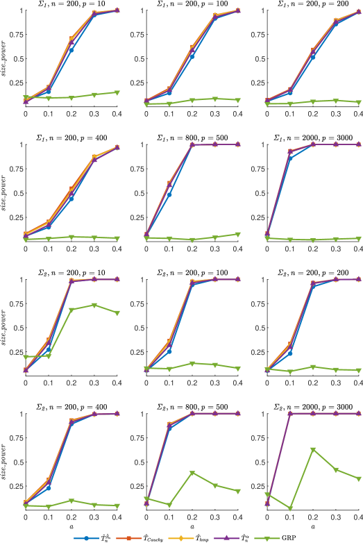
Figure 1: Empirical sizes and powers of the tests for $H_{21}$ in Study 2.

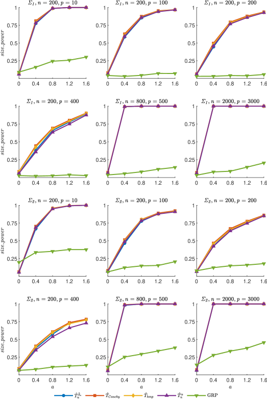
Figure 2: Empirical sizes and powers of the tests for $H_{22}$ in Study 2.

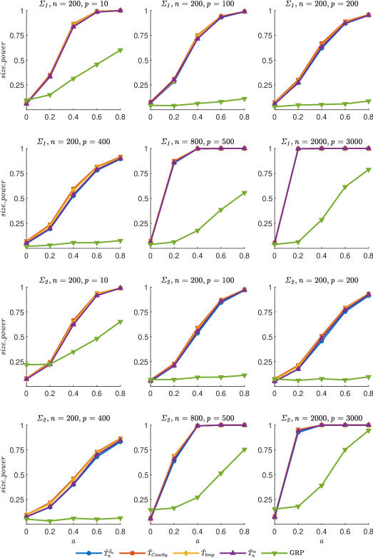
Figure 3: Empirical sizes and powers of the tests for $H_{23}$ in Study 2.

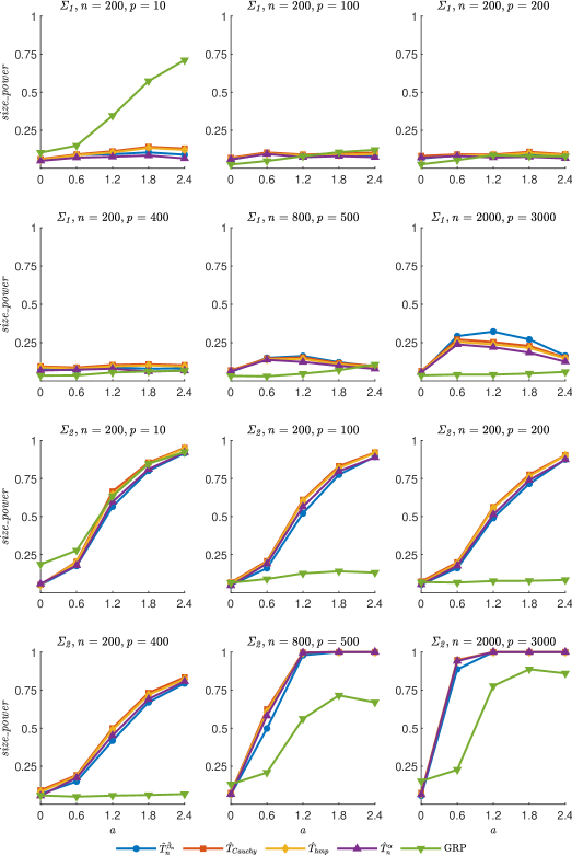
Figure 4: Empirical sizes and powers of the tests for $H_{24}$ in Study 2.

5.2 A real data example

In this subsection, we evaluate the proposed tests through an analysis of a classification task aimed at distinguishing between sonar signals bounced off a metal cylinder and those bounced off a roughly cylindrical rock. The dataset is available at https://archive.ics.uci.edu/dataset/151/connectionist+bench+sonar+mines+vs+rocks. There are 208 observations in this dataset collected by bouncing sonar signals off a metal cylinder or a roughly cylindrical rock. Each observation has 60 features ranging from $0$ to $1$, representing the energy within a particular frequency band, integrated over a certain period of time. Let $X=(X_{1},X_{2},\cdots,X_{60})$ represent the predictor vector and $Y$ be the response variable, where $Y=0$ if the signal is bounced off a metal cylinder and $Y=1$ if it is bounced off a roughly cylindrical rock. All predictor variables are standardize separately for easy explanation. We first check whether a sparse linear logistical regression model is adequate for a classification task. Then we apply our tests $\hat{T}_{n}^{\alpha}$, $\hat{T}_{n}^{\hat{\beta}}$, $\hat{T}_{hmp}$, and $\hat{T}_{Cauchy}$ to check whether $E(Y|X)=\exp{(\beta^{T}X)}/(1+\exp{(\beta^{T}X)})$ is plausible or not. The choice for the bandwidth $h$ and the projections are the same as in the simulation studies. The $p$-values of $\hat{T}_{n}^{\alpha}$, $\hat{T}_{n}^{\hat{\beta}}$, $\hat{T}_{hmp}$, and $\hat{T}_{Cauchy}$ are about $0.046$, $0.01$, $0.002$, and $0.002$, respectively, which indicate that a linear logistical regression model may be not adequate to fit this data. We then consider a quadratic logistical regression model by incorporating the squared predictors. Write $X_{new}=(X_{1},X_{2},\dots,X_{60},X_{1}^{2},X_{2}^{2},\dots,X_{60}^{2})$. When applying the proposed tests to the quadratic logistical regression model, the corresponding $p$-values of $\hat{T}_{n}^{\alpha}$, $\hat{T}_{n}^{\hat{\beta}}$, $\hat{T}_{hmp}$, and $\hat{T}_{Cauchy}$ are $0.723,0.688,0.933$, and $0.684$, respectively. This means that a quadratic logistical regression model may be plausible.

We further compare the predictive accuracy of the linear logistical regression model with the quadratic logistical regression model. We conducted $100$ runs to reduce the bias resulting from the randomness in selecting samples for the training and testing sets. In each run, the dataset was randomly shuffled and split into a training set ($80\%$) and a testing set ($20\%$). The models are estimated using the training set, and the predictive accuracy of these models is computed using the testing set. We then get an average predictive accuracy of $76.51\%$ for the quadratic logistical regression model, which is better than the linear logistical regression model with the accuracy of $72.46\%$. This confirms that a quadratic logistical regression model may be useful to fit this dataset.

6 Conclusion

This paper developed goodness of fit tests for checking generalized linear models when the dimension of covariates may substantially exceed the sample size. It is well known that existing goodness of fit tests for regressions in the literature usually cannot be extended to high dimension settings due to challenges arising from the “curse of dimensionality”, or dependencies on the normality of parameter estimators. While our tests do not depend on the asymptotic expansion or the normality of parameter estimators. We investigated the asymptotic properties of the proposed test statistics under the null and the alternatives, when the growing rate of the dimension $p$ is of exponential order in relation to the sample size. Further, our tests can detect the local alternative departing from the null at the rate of $n^{-1/2}h^{-1/4}$. As this detective rate is not related to the dimension $p$, the “curse of dimensionality” for our tests can be largely alleviated. The simulation results in Section 5 validates these theoretical results in finite samples. An interesting phenomenon is that for randomly chosen projections, the resulting test statistics may be asymptotic independent. This result can also be applied to other statistical problems based on random projections, such as high dimensional significant tests. However, employing random projections introduces variability in the values of the test statistics across various projections, even for the integrated tests $\hat{T}_{hmp}$ and $\hat{T}_{Cauchy}$. One potential solution is to utilize the optimal projection under the alternatives to construct the test statistics. Further, the data splitting is completely avoided when constructing our test statistic and deriving its asymptotic properties in high dimension settings. Thus, our method can be extended to develop goodness of fit tests for high-dimensional dependent data. This research is ongoing.

7 Supplementary Material

The Supplementary Material contains the technical lemmas and the proofs for the theoretical results presented in the main text of this paper.

7.1 Technical lemmas

In this subsection, we give some lemmas which will be used in the proofs of the theoretical results in the main text. Consider an $U$-statistic

$$U_{n}=\frac{2}{n(n-1)}\sum_{1\leq i<j\leq n}H(Z_{i},Z_{j}),$$

where the kernel function $H(\cdot,\cdot)$ is symmetric, and $Z_{i}$ and $H$ may depend on the sample size $n$. Let $G(x,y)=E[H(Z_{1},x)H(Z_{1},y)]$, $\sigma^{2}_{H}=var\{H(Z_{1},Z_{2})\}$, and $\sigma^{2}_{U_{n}}=var(U_{n})$.

Lemma 2.

Suppose $E[H(Z_{1},Z_{2})|Z_{1}]=0$ a.s. and $E[H^{2}(Z_{1},Z_{2})]<\infty$. If $\{E[G^{2}(Z_{1},Z_{2})]+n^{-1}E[H^{4}(Z_{1},Z_{2})]\}/[EH^{2}(Z_{1},Z_{2})]^{2}\to 0$ as $n\to\infty$, then

$$\frac{nU_{n}}{\{2E[H^{2}(Z_{1},Z_{2})]\}^{1/2}}\longrightarrow N(0,1),\quad{in\ distribution}.$$

Lemma 2 is a slightly modified version of Theorem 1 of Hall (1984) and its proof is based on the martingale central limit theorem, see Hall (1984) for more details. The next two lemmas will be used to bound the tail probability of random variables in high dimensional settings. Recall that a random variable $X\in\mathbb{R}$ is called sub-Weibull of order $\tau>0$, if

$$\|X\|_{\psi_{\tau}}:=\inf\{\eta>0:E\psi_{\tau}(\frac{|X|}{\eta})\leq 1\}<\infty,$$

where $\psi_{\tau}(x)=\exp(x^{\tau})-1$ for $x\geq 0$. The following lemma presents the tail probability for sums of independent sub-Weibull random variables of order $\tau$. Write $\|x\|_{p}=(\sum_{j=1}^{p}|x^{(i)}|^{p})^{1/p}$ for any $x=(x^{(1)},\cdots,x^{(p)})^{\top}\in\mathbb{R}^{p}$ and $p\geq 1$.

Lemma 3.

If $X_{1},\cdots,X_{n}$ are independent mean zero random variables in $\mathbb{R}$ with $\|X_{i}\|_{\psi_{\tau}}<\infty$ for all $1\leq i\leq n$ and some $\tau>0$, then we have

$$\mathbb{P}(|\frac{1}{n}\sum_{i=1}^{n}X_{i}|\geq a_{1\tau}\|\beta\|_{2}\sqrt{t}+a_{2\tau}\|\beta\|_{c(\tau)}t^{1/\tau})\leq 2\exp(-t),\quad\forall\ t\geq 0,$$

where $\beta=\frac{1}{n}(\|X_{1}\|_{\psi_{\tau}},\cdots,\|X_{n}\|_{\psi_{\tau}})^{\top}$, $a_{1\tau}$ and $a_{2\tau}$ are two constants relying only on $\tau$, $c(\tau)=\infty$ for $\tau\leq 1$, and $c(\tau)=\tau/(\tau-1)$ for $\tau>1$. By setting $u=a_{1\tau}\|\beta\|_{2}\sqrt{t}+a_{2\tau}\|\beta\|_{c(\tau)}t^{1/\tau}$, we have

$$\mathbb{P}(|\frac{1}{n}\sum_{i=1}^{n}X_{i}|>u)\leq 2\exp\left(-(\frac{u}{2a_{1\tau}\|\beta\|_{2}})^{2}\wedge(\frac{u}{2a_{2\tau}\|\beta\|_{c(\tau)}})^{\tau}\right),$$

where $s\wedge t=\min\{s,t\}$.

Lemma 3 is a variant of Theorem 3.4 in Kuchibhotla and Chakrabortty (2022) and its proof can be found in the Appendix of their paper. We may also need the results for the tail probability of $U$-statistics. Let $\Phi(x)$ denote the cumulative distribution function of a standard normal distribution.

Lemma 4.

Suppose that $E[H(Z_{1},Z_{2})]=0$ and $var\{E[H(Z_{1},Z_{2})|Z_{1}]\}>0$.
(1) If there exist a constant $C>0$ such that

$$E\exp\{tH(Z_{1},Z_{2})\}<\infty,\quad t\in[-C,C],$$

then, in the interval $0<x\leq o(n^{1/6})$, we have

$$\mathbb{P}\{\sigma_{U_{n}}^{-1}U_{n}<-x\} = \Phi(-x)(1+o(1)),$$

$$1-\mathbb{P}\{\sigma_{U_{n}}^{-1}U_{n}<x\} = [1-\Phi(x)](1+o(1)),\quad{\rm as}\ n\to\infty.$$ (7.1)

(2) If there exist two constants $C>0$ and $\gamma>0$ such that

$$E\exp\{t|H(Z_{1},Z_{2})|^{1/(1+\gamma)}\}<\infty,\quad t\in[-C,C],$$

then, in the interval $0<x\leq o(n^{\frac{1}{2(3+2\gamma)}})$, (4) continues to hold.

The results of Lemma 4 can be found in Theorems 1 and 2 of Aleshkyavichene (2006) (the notations may be different from here). Note that (4) implies that for $n$ large enough,

$$\mathbb{P}\{|\sigma_{U_{n}}^{-1}U_{n}|>x\}=[1-\Phi(x)](2+o(1))\leq C\exp(-\frac{x^{2}}{2}).$$

7.2 Lasso estimators under the null and alternative hypotheses

In this subsection, we investigate the convergence rate of the lasso estimators under the null (specified models) and alternative (misspecified models) when the dimension $p$ of covariates may be larger than the sample size $n$. Let $\hat{\beta}$ be the Lasso estimator of $\beta_{0}$ under the generalized linear model setting:

$$\hat{\beta}:=\mathop{\arg\min}\limits_{\beta\in\Theta\subset\mathbb{R}^{p}}\{L_{n}(\beta)+\lambda\sum_{j=1}^{p}|\beta^{(j)}|\},$$ (7.2)

where $L_{n}(\beta)=\frac{1}{n}\sum_{i=1}^{n}\rho(Y_{i},X_{i}^{\top}\beta)$, $\rho$ denotes some general loss function, and $\lambda>0$ is the regularization parameter. Write $L(\beta)=E[\rho(Y,X^{\top}\beta)]$ and

$$\tilde{\beta}_{0}=\mathop{\arg\min}\limits_{\beta\in\Theta\subset\mathbb{R}^{p}}L(\beta).$$

For simplicity, we focus on Gaussian linear models in this paper with the square loss function

$$\rho(Y,\beta^{\top}X)=(Y-\beta^{\top}X)^{2}.$$

The extension for lasso estimators for generalized linear models with general loss function in high dimension settings can be similar. Note that under the null hypothesis $H_{0}$, the linear model is correctly specified for some true parameter $\beta_{0}$. It is easy to see that $\tilde{\beta}_{0}=\beta_{0}$ under the null $H_{0}$. While under the alternative hypotheses $H_{1}$, the linear model is misspecified with a pseudo-parameter $\tilde{\beta}_{0}$. Suppose $\tilde{\beta}_{0}$ is unique and lies in the interior of $\Theta$.

To investigate the convergence rate of $\hat{\beta}-\tilde{\beta}_{0}$ under both the null $H_{0}$ and the alternative $H_{1}$, we introduce some notations and conditions. Write

$$W(\beta) = L(\beta)-L(\tilde{\beta}_{0}),$$

$$W_{n}(\beta) = L_{n}(\beta)-L_{n}(\tilde{\beta}_{0}),$$

$$W_{d}(r) = \sup_{\|\beta-\tilde{\beta}_{0}\|_{1}\leq r}|W_{n}(\beta)-W(\beta)|.$$

Recall that $\tilde{S}=\{j:\tilde{\beta}_{0}^{(j)}\neq 0,1\leq j\leq p\}$ be the support of $\tilde{\beta}_{0}$ and $\tilde{s}=|\tilde{S}|$. Consider cones of the form

$$\mathcal{C}_{\epsilon}=\{\Delta\in\mathbb{R}^{p}:\|\Delta_{\tilde{S}^{c}}\|_{1}\leq\epsilon\|\Delta_{\tilde{S}}\|_{1}\},$$

where $\epsilon>0$. We need the following Compatibility Condition (CC) to derive the asymptotic properties of $\hat{\beta}$.

(CC) For the set $\tilde{S}$, there exists a constant $\phi_{\tilde{S}}\geq C>0$ such that

$$\|\beta_{\tilde{S}}\|_{1}^{2}\leq\frac{\tilde{s}\beta^{\top}E[XX^{\top}]\beta}{\phi_{\tilde{S}}^{2}},\quad{\rm for\ all}\ \beta\in\mathcal{C}_{2},$$

where $C$ is a constant independent of $n$. The Compatibility Condition (CC) is usually imposed in the literature for investigating the asymptotic properties of lasso estimators, see Chapter 6 of Bühlmann and Van De Geer (2011) for instance. Write $\epsilon^{*}=\tilde{s}\lambda^{2}/\phi_{\tilde{S}}$, $r=\epsilon^{*}/\lambda_{0}$, and define an event

$$\mathcal{F}=\{W_{d}(r)\leq\epsilon^{*}\}=\{W_{d}(r)\leq r\lambda_{0}\}.$$

Lemma 5.

Suppose the Compatibility Condition (CC) holds for $\tilde{S}$. If $\lambda\geq 6\lambda_{0}$, then on the event $\mathcal{F}=\{W_{d}(r)\leq\epsilon^{*}\}$, we have

$$\frac{L(\hat{\beta})-L(\tilde{\beta}_{0})}{2}+\lambda\|\hat{\beta}-\tilde{\beta}_{0}\|_{1}\leq 3\epsilon^{*}.$$

Proof of Lemma 5. Write $t=\frac{r}{r+\|\hat{\beta}-\tilde{\beta}_{0}\|_{1}}$ and $u=t\hat{\beta}+(1-t)\tilde{\beta}_{0}$. It is easy to see that $\|u-\tilde{\beta}_{0}\|_{1}\leq r$. By the convexity of $L_{n}(\beta)+\lambda\|\beta\|_{1}$, we have

$$L_{n}(u)+\lambda\|u\|_{1}\leq L_{n}(\tilde{\beta}_{0})+\lambda\|\tilde{\beta}_{0}\|_{1}.$$

Then on this event $\mathcal{F}=\{W_{d}(r)\leq\epsilon^{*}\}$,

$$L(u)-L(\tilde{\beta}_{0})+\lambda\|u\|_{1}\leq W(u)-W_{n}(u)+\lambda\|\tilde{\beta}_{0}\|_{1}\leq W_{d}(r)+\lambda\|\tilde{\beta}_{0}\|_{1}\leq\epsilon^{*}+\lambda\|\tilde{\beta}_{0}\|_{1}.$$

Note that $\tilde{\beta}_{0\tilde{S}^{c}}=0$, so we have

$$L(u)-L(\tilde{\beta}_{0})+\lambda(\|u_{\tilde{S}}\|_{1}+\|u_{\tilde{S}^{c}}\|_{1})\leq\epsilon^{*}+\lambda\|\tilde{\beta}_{0\tilde{S}}\|_{1},$$

whence

$$L(u)-L(\tilde{\beta}_{0})+\lambda\|u_{\tilde{S}^{c}}\|_{1}\leq\epsilon^{*}+\lambda\|u_{\tilde{S}}-\tilde{\beta}_{0\tilde{S}}\|_{1}.$$ (7.3)

Next we complete this proof by considering two cases.

Case (i). If $\lambda\|u_{\tilde{S}}-\tilde{\beta}_{0\tilde{S}}\|_{1}\geq\epsilon^{*}$, it follows from (7.3) that

$$L(u)-L(\tilde{\beta}_{0})+\lambda\|u_{\tilde{S}^{c}}\|_{1}\leq 2\lambda\|u_{\tilde{S}}-\tilde{\beta}_{0\tilde{S}}\|_{1}.$$

So $\|u_{\tilde{S}^{c}}\|_{1}=\|u_{\tilde{S}^{c}}-\tilde{\beta}_{0\tilde{S}^{c}}\|_{1}\leq 2\|u_{\tilde{S}}-\tilde{\beta}_{0\tilde{S}}\|_{1}$ and then $u-\tilde{\beta}_{0}\in\mathcal{C}_{2}$. Also note that $\|u-\tilde{\beta}_{0}\|_{1}=\|u_{\tilde{S}}-\tilde{\beta}_{0\tilde{S}}\|_{1}+\|u_{\tilde{S}^{c}}\|_{1}$, using (7.3) again, we have

$$L(u)-L(\tilde{\beta}_{0})+\lambda\|u-\tilde{\beta}_{0}\|_{1}\leq\epsilon^{*}+2\lambda\|u_{\tilde{S}}-\tilde{\beta}_{0\tilde{S}}\|_{1}.$$

As $u-\tilde{\beta}_{0}\in\mathcal{C}_{2}$, it follows from the Compatibility Condition (CC) that

$$L(u)-L(\tilde{\beta}_{0})+\lambda\|u-\tilde{\beta}_{0}\|_{1} \leq \epsilon^{*}+2\lambda\|u_{\tilde{S}}-\tilde{\beta}_{0\tilde{S}}\|_{1}$$

$$\leq \epsilon^{*}+2\lambda\frac{\sqrt{\tilde{s}(u-\tilde{\beta}_{0})^{\top}E[XX^{\top}](u-\tilde{\beta}_{0})}}{\phi_{\tilde{S}}}$$

$$\leq \epsilon^{*}+\frac{2\tilde{s}\lambda^{2}}{\phi_{\tilde{S}}^{2}}+\frac{(u-\tilde{\beta}_{0})^{\top}E[XX^{\top}](u-\tilde{\beta}_{0})}{2}$$

$$= 3\epsilon^{*}+\frac{(u-\tilde{\beta}_{0})^{\top}E[XX^{\top}](u-\tilde{\beta}_{0})}{2}.$$

Recall that $E(Y-\tilde{\beta}_{0}^{\top}X)X=0$, then for any $\beta$,

$$L(\beta)-L(\tilde{\beta}_{0}) = E(Y-\beta^{\top}X)^{2}-E(Y-\tilde{\beta}_{0}^{\top}X)^{2}$$

$$= E(\beta^{\top}X-\tilde{\beta}_{0}^{\top}X)^{2}$$

$$= (\beta-\tilde{\beta}_{0})^{\top}E(XX^{\top})(\beta-\tilde{\beta}_{0})$$

Consequently,

$$\frac{L(u)-L(\tilde{\beta}_{0})}{2}+\lambda\|u-\tilde{\beta}_{0}\|_{1}\leq 3\epsilon^{*}.$$

We also obtain that

$$\|u-\tilde{\beta}_{0}\|_{1}\leq\frac{3\epsilon^{*}}{\lambda}=\frac{3r\lambda_{0}}{\lambda}\leq\frac{r}{2}.\quad({\rm since}\ \lambda\geq 6\lambda_{0})$$

Also note that

$$\|u-\tilde{\beta}_{0}\|_{1}=t\|\hat{\beta}-\tilde{\beta}_{0}\|_{1}=\frac{r}{r+\|\hat{\beta}-\tilde{\beta}_{0}\|_{1}}\|\hat{\beta}-\tilde{\beta}_{0}\|_{1}\leq\frac{r}{2},$$

some elementary calculations show that $\|\hat{\beta}-\tilde{\beta}_{0}\|_{1}\leq r$. Then we can replace $u$ by $\hat{\beta}$ in the above process and obtain the result

$$\frac{L(\hat{\beta})-L(\tilde{\beta}_{0})}{2}+\lambda\|\hat{\beta}-\tilde{\beta}_{0}\|_{1}\leq 3\epsilon^{*}.$$

Case (ii). If $\lambda\|u_{\tilde{S}}-\tilde{\beta}_{0\tilde{S}}\|_{1}<\epsilon^{*}$, then by (7.3), we have

$$L(u)-L(\tilde{\beta}_{0})+\lambda\|u_{\tilde{S}^{c}}\|_{1}\leq\epsilon^{*}+\lambda\|u_{\tilde{S}}-\tilde{\beta}_{0\tilde{S}}\|_{1}\leq 2\epsilon^{*}.$$

As $\|u-\tilde{\beta}_{0}\|_{1}=\|u_{\tilde{S}}-\tilde{\beta}_{0\tilde{S}}\|_{1}+\|u_{\tilde{S}^{c}}\|_{1}$, it follows that

$$\frac{L(u)-L(\tilde{\beta}_{0})}{2}+\lambda\|u-\tilde{\beta}_{0}\|_{1}\leq L(u)-L(\tilde{\beta}_{0})+\lambda\|u-\tilde{\beta}_{0}\|_{1}\leq 3\epsilon^{*}.$$

Similar to the arguments in Case (i), we have

$$\frac{L(\hat{\beta})-L(\tilde{\beta}_{0})}{2}+\lambda\|\hat{\beta}-\tilde{\beta}_{0}\|_{1}\leq 3\epsilon^{*}.$$

Combining the results in the Cases (i) and (ii), we reach the result of this lemma. $\Box$

Next we investigate the probability of the event $\mathcal{F}=\{W_{d}(r)\leq\epsilon^{*}\}=\{W_{d}(r)\leq r\lambda_{0}\}$. Let $\varepsilon_{i}(\tilde{\beta}_{0})=Y_{i}-\tilde{\beta}_{0}^{\top}X_{i}$ and $X_{i}^{(j)}$ denotes the $j$-th component of $X_{i}$.

Lemma 6.

Suppose $\varepsilon_{i}(\tilde{\beta}_{0})$ and $X_{i}^{(j)}$ are sub-Weibull of order $2$ for all $1\leq i\leq n,1\leq j\leq p$. Then we have

$$\mathbb{P}\{W_{d}(r)>\epsilon^{*}\} \leq 2\exp\left(-\frac{n{\epsilon^{*}}^{2}}{Cr^{4}}+2\log{p}\right)\vee 2\exp\left(-\frac{n\epsilon^{*}}{Cr^{2}}+2\log{p}\right)$$

$$+2\exp\left(-\frac{n{\epsilon^{*}}^{2}}{Cr^{2}}+\log{p}\right)\vee 2\exp\left(-\frac{n\epsilon^{*}}{Cr}+\log{p}\right).$$

Proof of Lemma 6. Recall that $W_{d}(r)=\sup_{\|\beta-\tilde{\beta}_{0}\|_{1}\leq r}|W_{n}(\beta)-W(\beta)|$ with

$$W(\beta) = E(Y-\beta^{\top}X)^{2}-E(Y-\tilde{\beta}_{0}^{\top}X)^{2},$$

$$W_{n}(\beta) = \frac{1}{n}\sum_{i=1}^{n}(Y_{i}-\beta^{\top}X_{i})^{2}-\frac{1}{n}\sum_{i=1}^{n}(Y_{i}-\tilde{\beta}_{0}^{\top}X_{i})^{2}.$$

Note that $E[(Y-\tilde{\beta}_{0}^{\top}X)X]=0$, it is easy to see that

$$W_{d}(r)=\sup_{\|\beta-\tilde{\beta}_{0}\|_{1}\leq r}\big{|}\frac{1}{n}\sum_{i=1}^{n}\{(\beta^{\top}X_{i}-\tilde{\beta}_{0}^{\top}X_{i})^{2}-E(\beta^{\top}X-\tilde{\beta}_{0}^{\top}X)^{2}-2\varepsilon_{i}(\tilde{\beta}_{0})(\beta^{\top}X_{i}-\tilde{\beta}_{0}^{\top}X_{i})\}\big{|},$$

where $\varepsilon_{i}(\tilde{\beta}_{0})=Y_{i}-\tilde{\beta}_{0}^{\top}X_{i}$. Consequently,

$$\mathbb{P}\{W_{d}(r)>\epsilon^{*}\}$$

$$= \mathbb{P}\left(\sup_{\|\beta-\tilde{\beta}_{0}\|_{1}\leq r}\big{|}\frac{1}{n}\sum_{i=1}^{n}\{(\beta^{\top}X_{i}-\tilde{\beta}_{0}^{\top}X_{i})^{2}-E(\beta^{\top}X-\tilde{\beta}_{0}^{\top}X)^{2}-2\varepsilon_{i}(\tilde{\beta}_{0})(\beta^{\top}X_{i}-\tilde{\beta}_{0}^{\top}X_{i})\}\big{|}>\epsilon^{*}\right)$$

$$\leq \mathbb{P}\left(\sup_{\|\beta-\tilde{\beta}_{0}\|_{1}\leq r}\big{|}\frac{1}{n}\sum_{i=1}^{n}[(\beta^{\top}X_{i}-\tilde{\beta}_{0}^{\top}X_{i})^{2}-E(\beta^{\top}X-\tilde{\beta}_{0}^{\top}X)^{2}]\big{|}>\frac{\epsilon^{*}}{2}\right)$$

$$+\mathbb{P}\left(\sup_{\|\beta-\tilde{\beta}_{0}\|_{1}\leq r}\big{|}\frac{1}{n}\sum_{i=1}^{n}\varepsilon_{i}(\tilde{\beta}_{0})(\beta^{\top}X_{i}-\tilde{\beta}_{0}^{\top}X_{i})\big{|}>\frac{\epsilon^{*}}{4}\right)$$

$$\leq \mathbb{P}\left(\sup_{\|\beta-\tilde{\beta}_{0}\|_{1}\leq r}\|\beta-\tilde{\beta}_{0}\|_{1}^{2}\max_{1\leq k,l\leq p}|\frac{1}{n}\sum_{i=1}^{n}(X_{i}^{(k)}X_{i}^{(l)}-EX_{i}^{(k)}X_{i}^{(l)})|>\frac{\epsilon^{*}}{2}\right)$$

$$+\mathbb{P}\left(\sup_{\|\beta-\tilde{\beta}_{0}\|_{1}\leq r}\|\beta-\tilde{\beta}_{0}\|_{1}\max_{1\leq k\leq p}\big{|}\frac{1}{n}\sum_{i=1}^{n}\varepsilon_{i}(\tilde{\beta}_{0})X_{i}^{(k)}|>\frac{\epsilon^{*}}{4}\right)$$

$$\leq \mathbb{P}\left(\max_{1\leq k,l\leq p}|\frac{1}{n}\sum_{i=1}^{n}(X_{i}^{(k)}X_{i}^{(l)}-EX_{i}^{(k)}X_{i}^{(l)})\big{|}>\frac{\epsilon^{*}}{2r^{2}}\right)+\mathbb{P}\left(\max_{1\leq k\leq p}|\frac{1}{n}\sum_{i=1}^{n}\varepsilon_{i}(\tilde{\beta}_{0})X_{i}^{(k)}|>\frac{\epsilon^{*}}{4r}\right)$$

$$\leq \sum_{k,l=1}^{p}\mathbb{P}\left(|\frac{1}{n}\sum_{i=1}^{n}(X_{i}^{(k)}X_{i}^{(l)}-EX_{i}^{(k)}X_{i}^{(l)})|>\frac{\epsilon^{*}}{2r^{2}}\right)+\sum_{k=1}^{p}\mathbb{P}\left(|\frac{1}{n}\sum_{i=1}^{n}\varepsilon_{i}(\tilde{\beta}_{0})X_{i}^{(k)}|>\frac{\epsilon^{*}}{4r}\right)$$

$$=: I_{1}+I_{2}.$$

For $I_{1}$, note that $X_{i}^{(k)}$ is sub-Weibull of order $2$ with $\|X_{i}^{(k)}\|_{\psi_{2}}\leq C<\infty$ for all $k=1,\cdots,p$. According to Proposition D.2 of Kuchibhotla and Chakrabortty (2022), we have

$$\|X_{i}^{(k)}X_{i}^{(l)}\|_{\psi_{1}}\leq\|X_{i}^{(k)}\|_{\psi_{2}}\|X_{i}^{(l)}\|_{\psi_{2}}.$$

This means that $X_{i}^{(k)}X_{i}^{(l)}$ is sub-Weibull of order $\tau=1$ with $\|X_{i}^{(k)}X_{i}^{(l)}\|_{\psi_{1}}\leq C<\infty$ and so is $X_{i}^{(k)}X_{i}^{(l)}-E(X_{i}^{(k)}X_{i}^{(l)})$ for all $k,l$. Applying Lemma 3, we have

$$\mathbb{P}\left(|\frac{1}{n}\sum_{i=1}^{n}(X_{i}^{(k)}X_{i}^{(l)}-EX_{i}^{(k)}X_{i}^{(l)})|>\frac{\epsilon^{*}}{2r^{2}}\right)$$

$$\leq 2\exp\left(-\frac{n|\epsilon^{*}/(2r^{2})|^{2}}{4a_{1\tau}^{2}\|X_{i}^{(k)}X_{i}^{(l)}-E(X_{i}^{(k)}X_{i}^{(l)})\|^{2}_{\psi_{\tau}}}\wedge\frac{n\epsilon^{*}/(2r^{2})}{2a_{2\tau}\|X_{i}^{(k)}X_{i}^{(l)}-E(X_{i}^{(k)}X_{i}^{(l)})\|_{\psi_{\tau}}}\right)$$

$$\leq 2\exp\left(-\frac{n{\epsilon^{*}}^{2}}{Cr^{4}}\wedge\frac{n\epsilon^{*}}{Cr^{2}}\right)$$

$$= 2\exp\left(-\frac{n{\epsilon^{*}}^{2}}{Cr^{4}}\right)\vee 2\exp\left(-\frac{n\epsilon^{*}}{Cr^{2}}\right),$$

where $a\vee b=\max\{a,b\}$ and $a\wedge b=\min\{a,b\}$. Consequently,

$$I_{1} \leq 2p^{2}\exp\left(-\frac{n{\epsilon^{*}}^{2}}{Cr^{4}}\right)\vee 2p^{2}\exp\left(-\frac{n\epsilon^{*}}{Cr^{2}}\right)$$

$$= 2\exp\left(-\frac{n{\epsilon^{*}}^{2}}{Cr^{4}}+2\log{p}\right)\vee 2\exp\left(-\frac{n\epsilon^{*}}{Cr^{2}}+2\log{p}\right).$$

Similarly, we can show that

$$I_{2}=\sum_{k=1}^{p}\mathbb{P}\left(|\frac{1}{n}\sum_{i=1}^{n}\varepsilon_{i}(\tilde{\beta}_{0})X_{i}^{(k)}|>\frac{\epsilon^{*}}{4r}\right)\leq 2\exp\left(-\frac{n{\epsilon^{*}}^{2}}{Cr^{2}}+\log{p}\right)\vee 2\exp\left(-\frac{n\epsilon^{*}}{Cr}+\log{p}\right).$$

Altogether we obtain that

$$\mathbb{P}\{W_{d}(r)>\epsilon^{*}\} \leq 2\exp\left(-\frac{n{\epsilon^{*}}^{2}}{Cr^{4}}+2\log{p}\right)\vee 2\exp\left(-\frac{n\epsilon^{*}}{Cr^{2}}+2\log{p}\right)$$

$$+2\exp\left(-\frac{n{\epsilon^{*}}^{2}}{Cr^{2}}+\log{p}\right)\vee 2\exp\left(-\frac{n\epsilon^{*}}{Cr}+\log{p}\right).$$

Hence we complete the proof of this lemma. $\Box$

Based on Lemmas 5 and 6, we can derive the convergence rate of the lasso estimators $\hat{\beta}$ under the null (specified models) and alternative (misspecified models) when the dimension $p$ of covariates may be larger than the sample size $n$.

Corollary 3.

Suppose that the conditions in Lemmas 5 and 6 hold. If $\lambda_{\min}(E(XX^{\top}))\geq C>0$, $(\tilde{s}^{2}\log{p})/n=o(1)$ as $n\to\infty$, and the tuning parameter $\lambda$ satisfies $\lambda=O(\sqrt{\log{p}/n})$, then we have

$$\|\hat{\beta}-\tilde{\beta}_{0}\|_{1}=O_{p}(\tilde{s}\sqrt{\frac{\log{p}}{n}})\quad{\rm and}\quad\|\hat{\beta}-\tilde{\beta}_{0}\|_{2}=O_{p}(\sqrt{\frac{\tilde{s}\log{p}}{n}}).$$

Proof of Corollary 3. First we investigate the convergence rate of $\|\hat{\beta}-\tilde{\beta}_{0}\|_{1}$. Let $\lambda=6\lambda_{0}$ and $\lambda_{0}=C_{1}\sqrt{\frac{\log{p}}{n}}$ for some positive constant $C_{1}$ large enough. By Lemma 5, we have

$$\mathcal{F}=\{W_{d}(r)\leq\epsilon^{*}\}\subset\{\|\hat{\beta}-\tilde{\beta}_{0}\|_{1}\leq 3\epsilon^{*}/\lambda\}$$

Recall that $\epsilon^{*}=\frac{\tilde{s}\lambda^{2}}{\phi_{\tilde{S}}}=\frac{36\tilde{s}\lambda_{0}^{2}}{\phi_{\tilde{S}}}$ and $r=\frac{\epsilon^{*}}{\lambda_{0}}=\frac{36\tilde{s}\lambda_{0}}{\phi_{\tilde{S}}}$, it follows from Lemma 6 that

$$\mathbb{P}\{\|\hat{\beta}-\tilde{\beta}_{0}\|_{1}\geq\frac{18\tilde{s}\lambda_{0}}{\phi_{\tilde{S}}}\} = \mathbb{P}\{\|\hat{\beta}-\tilde{\beta}_{0}\|_{1}>3\epsilon^{*}/\lambda\}$$

$$\leq \mathbb{P}\{W_{d}(r)>\epsilon^{*}\}$$

$$\leq 2\exp\left(-\frac{n{\epsilon^{*}}^{2}}{Cr^{4}}+2\log{p}\right)\vee 2\exp\left(-\frac{n\epsilon^{*}}{Cr^{2}}+2\log{p}\right)$$

$$+2\exp\left(-\frac{n{\epsilon^{*}}^{2}}{Cr^{2}}+\log{p}\right)\vee 2\exp\left(-\frac{n\epsilon^{*}}{Cr}+\log{p}\right)\quad\epsilon^{*}=r\lambda_{0}$$

$$= 2\exp\left(-\frac{n\phi_{\tilde{S}}^{2}}{C\tilde{s}^{2}}+2\log{p}\right)\vee\exp\left(-\frac{\phi_{\tilde{S}}n}{C\tilde{s}}+2\log{p}\right)$$

$$+2\exp\left(-\frac{C_{1}^{2}\log{p}}{C}+\log{p}\right)\vee\exp\left(-\frac{C_{1}\sqrt{n\log{p}}}{C}+\log{p}\right)$$

$$= o(1),\quad{\rm as}\ \frac{\tilde{s}^{2}\log{p}}{n}=o(1)\ {\rm and}\ C_{1}\ {\rm large\ enough}.$$

Then we have $\|\hat{\beta}-\tilde{\beta}_{0}\|_{1}=O_{p}(\tilde{s}\sqrt{\frac{\log{p}}{n}})$.

For $\|\hat{\beta}-\tilde{\beta}_{0}\|_{2}$, according to Lemma 5, we have on the event $\mathcal{F}=\{W_{d}(r)\leq\epsilon^{*}\}$,

$$\frac{L(\hat{\beta})-L(\tilde{\beta}_{0})}{2}+\lambda\|\hat{\beta}-\tilde{\beta}_{0}\|_{1}\leq 3\epsilon^{*}.$$

Note that

$$L(\hat{\beta})-L(\tilde{\beta}_{0})=(\hat{\beta}-\tilde{\beta}_{0})^{\top}E(XX^{\top})(\hat{\beta}-\tilde{\beta}_{0})\geq\lambda_{\min}(E(XX^{\top}))\|\hat{\beta}-\tilde{\beta}_{0}\|_{2}^{2},$$

it follows that

$$\mathcal{F}=\{W_{d}(r)\leq\epsilon^{*}\}\subset\{\|\hat{\beta}-\tilde{\beta}_{0}\|_{2}^{2}\leq\frac{6\epsilon^{*}}{\lambda_{\min}(E(XX^{\top}))}\}.$$

Recall that $\epsilon^{*}=\frac{\tilde{s}\lambda^{2}}{\phi_{\tilde{S}}}=\frac{36\tilde{s}\lambda_{0}^{2}}{\phi_{\tilde{S}}}$ and $\lambda_{0}=C_{1}\sqrt{\frac{\log{p}}{n}}$ for some positive constant $C_{1}$ large enough. Similar to the arguments for $\|\hat{\beta}-\tilde{\beta}_{0}\|_{1}$, we have

$$\mathbb{P}\{\|\hat{\beta}-\tilde{\beta}_{0}\|_{2}^{2}>\frac{6\epsilon^{*}}{\lambda_{\min}(E(XX^{\top}))}\}\leq\mathbb{P}\{W_{d}(r)>\epsilon^{*}\}=o(1),$$

for $C_{1}$ large enough. Thus, we obtain that $\|\hat{\beta}-\tilde{\beta}_{0}\|_{2}=\sqrt{\frac{\tilde{s}\log{p}}{n}}$. This completes the proof of Corollary 3. $\Box$

Recall that $\tilde{\beta}_{0}=\beta_{0}$ and $\tilde{s}=s$ under the null $H_{0}$, then we have

$$\|\hat{\beta}-\beta_{0}\|_{1}=O_{p}(s\sqrt{\frac{\log{p}}{n}})\quad{\rm and}\quad\|\hat{\beta}-\beta_{0}\|_{2}=O_{p}(\sqrt{\frac{s\log{p}}{n}}).$$

Now we investigate the convergence rate of $\|\hat{\beta}-\beta_{0}\|_{1}$ and $\|\hat{\beta}-\beta_{0}\|_{2}$ under the local alternatives $H_{1n}$. Recall that

$$H_{1n}:m(x)=E(Y|X=x)=\beta_{0}^{\top}x+r_{n}R(x),$$

where $r_{n}\to 0$, and $R(\cdot)$ is a nonlinear function with $\mathbb{P}(R(X)=0)<1$. Let $\tilde{S}_{1}=S\cup\tilde{S}$, $\tilde{s}=|\tilde{S}|$, $\tilde{s}_{1}=|\tilde{S}_{1}|$, and $\varepsilon(\beta_{0})=Y-E[Y|X]=Y-\beta_{0}^{\top}X-r_{n}R(X)$ under $H_{1n}$, where $S$ and $\tilde{S}$ are the supports of $\beta_{0}$ and $\tilde{\beta}_{0}$, respectively. Recall that

$$W_{d}(r)=\sup_{\|\beta-\tilde{\beta}_{0}\|_{1}\leq r}|L_{n}(\beta)-L_{n}(\tilde{\beta}_{0})-[L(\beta)-L(\tilde{\beta}_{0})]|,$$

where $L_{n}(\beta)=n^{-1}\sum_{i=1}^{n}(Y_{i}-\beta^{\top}X_{i})^{2}$ and $L(\beta)=E(Y-\beta^{\top}X)^{2}$. Write $\epsilon^{*}=\frac{\tilde{s}\lambda^{2}}{\phi_{\tilde{S}}}$, $r=\epsilon^{*}/\lambda_{0}$, and $\mathcal{F}=\{W_{d}(r)\leq\epsilon^{*}\}$.

Lemma 7.

Suppose the Compatibility Condition (CC) holds for the set $\tilde{S}$. If $\lambda\geq 6\lambda_{0}$, then on the event $\mathcal{F}=\{W_{d}(r)\leq\epsilon^{*}\}$ and under the local alternatives $H_{1n}$ with $r_{n}\to 0$, we have

$$\frac{L(\hat{\beta})-L(\tilde{\beta}_{0})}{2}+\lambda\|\hat{\beta}-\tilde{\beta}_{0}\|_{1}\leq 3\epsilon^{*}.$$

Proof of Lemma 7. The proof of this lemma is exactly the same as that of Lemma 6. Thus we omit the details here. $\Box$

Corollary 4.

Suppose $\varepsilon_{i}(\tilde{\beta}_{0})$ and $X_{i}^{(j)}$ are sub-Weibull of order $2$ for all $1\leq i\leq n,1\leq j\leq p$ and the Compatibility Condition (CC) holds for $\tilde{S}$. If $\lambda_{\min}(E(XX^{\top}))\geq C>0$, $(\tilde{s}^{2}\log{p})/n=o(1)$ as $n\to\infty$, and the tuning parameter $\lambda$ satisfies $\lambda=O(\sqrt{\log{p}/n})$, then under the local alternative $H_{1n}$ with $r_{n}\to 0$, we have

$$\|\hat{\beta}-\beta_{0}\|_{1} = O_{p}(\sqrt{\frac{\tilde{s}^{2}\log{p}}{n}}+r_{n}\sqrt{\tilde{s}_{1}}),$$

$$\|\hat{\beta}-\beta_{0}\|_{2} = O_{p}(\sqrt{\frac{\tilde{s}\log{p}}{n}}+r_{n}),$$

where $\tilde{s}=\tilde{S}$ and $\tilde{s}_{1}=|\tilde{S}_{1}|=|S\cup\tilde{S}|$.

Proof of Corollary 4. Recall that $E[(Y-\tilde{\beta}_{0}^{\top}X)X]=0$, $E[\varepsilon(\beta_{0})|X]=0$, $\beta_{0\tilde{S}_{1}^{c}}=0$ and $\tilde{\beta}_{0\tilde{S}_{1}^{c}}=0$ under the local alternatives $H_{1n}$, it follows that

$$0 = EX_{\tilde{S}_{1}}(Y-X_{\tilde{S}_{1}}^{\top}\tilde{\beta}_{0\tilde{S}_{1}})$$

$$= EX_{\tilde{S}_{1}}[X_{\tilde{S}_{1}}^{\top}(\beta_{0\tilde{S}_{1}}-\tilde{\beta}_{0\tilde{S}_{1}})+r_{n}R(X)+\varepsilon(\beta_{0})]$$

$$= E(X_{\tilde{S}_{1}}X_{\tilde{S}_{1}}^{\top})(\beta_{0\tilde{S}_{1}}-\tilde{\beta}_{0\tilde{S}_{1}})+r_{n}E[X_{\tilde{S}_{1}}R(X)],$$

whence

$$\beta_{0\tilde{S}_{1}}-\tilde{\beta}_{0\tilde{S}_{1}}=r_{n}\Sigma_{\tilde{S}_{1}}^{-1}E[X_{\tilde{S}_{1}}R(X)],$$

where $\Sigma_{\tilde{S}_{1}}=E(X_{\tilde{S}_{1}}X_{\tilde{S}_{1}}^{\top})$. Combining this with Lemma 7 and the Cauchy-Schwarz inequality, it follows that on the event $\mathcal{F}=\{W_{d}(r)\leq\epsilon^{*}\}$ and under the local alternatives $H_{1n}$,

$$\frac{L(\hat{\beta})-L(\tilde{\beta}_{0})}{2}+\lambda\|\hat{\beta}-\beta_{0}\|_{1} \leq 3\epsilon^{*}+\lambda\|\tilde{\beta}_{0}-\beta_{0}\|_{1}$$

$$= 3\epsilon^{*}+\lambda\|\beta_{0\tilde{S}_{1}}-\tilde{\beta}_{0\tilde{S}_{1}}\|_{1}$$

$$= 3\epsilon^{*}+\lambda r_{n}\|\Sigma_{\tilde{S}_{1}}^{-1}E[X_{\tilde{S}_{1}}R(X)]\|_{1}.$$

Thus, under the local alternative $H_{1n}$, we have

$$\mathcal{F}=\{W_{d}(r)\leq\epsilon^{*}\}\subset\{\|\hat{\beta}-\beta_{0}\|_{1}\leq 3\epsilon^{*}/\lambda+r_{n}\|\Sigma_{\tilde{S}_{1}}^{-1}E[X_{\tilde{S}_{1}}R(X)]\|_{1}\},$$

whence

$$\mathbb{P}\{\|\hat{\beta}-\beta_{0}\|_{1}>3\epsilon^{*}/\lambda+r_{n}\|\Sigma_{\tilde{S}_{1}}^{-1}E[X_{\tilde{S}_{1}}R(X)]\|_{1}\}\leq\mathbb{P}\{W_{d}(r)>\epsilon^{*}\}.$$

Let $\lambda=6\lambda_{0}$ and $\lambda_{0}=C_{1}\sqrt{\frac{\log{p}}{n}}$ for some positive constant $C_{1}$ large enough, then we have $\epsilon^{*}=\frac{\tilde{s}\lambda^{2}}{\phi_{\tilde{S}}}=\frac{36\tilde{s}\lambda_{0}^{2}}{\phi_{\tilde{S}}}$ and $r=\frac{\epsilon^{*}}{\lambda_{0}}=\frac{36\tilde{s}\lambda_{0}}{\phi_{\tilde{S}}}$. Similar to the arguments for Corollary 3, we can show that under the local alternative $H_{1n}$, if $\frac{\tilde{s}^{2}\log{p}}{n}=o(1)$, then

$$\mathbb{P}\{\|\hat{\beta}-\beta_{0}\|_{1}>3\epsilon^{*}/\lambda+r_{n}\|\Sigma_{\tilde{S}_{1}}^{-1}E[X_{\tilde{S}_{1}}R(X)]\|_{1}\}$$

$$\leq \mathbb{P}\{W_{d}(r)>\epsilon^{*}\}$$

$$\leq 2\exp\left(-\frac{n{\epsilon^{*}}^{2}}{Cr^{4}}+2\log{p}\right)\vee 2\exp\left(-\frac{n\epsilon^{*}}{Cr^{2}}+2\log{p}\right)$$

$$+2\exp\left(-\frac{n{\epsilon^{*}}^{2}}{Cr^{2}}+\log{p}\right)\vee 2\exp\left(-\frac{n\epsilon^{*}}{Cr}+\log{p}\right)$$

$$= 2\exp\left(-\frac{n\phi_{\tilde{S}}^{2}}{C\tilde{s}^{2}}+2\log{p}\right)\vee\exp\left(-\frac{\phi_{\tilde{S}}n}{C\tilde{s}}+2\log{p}\right)$$

$$+2\exp\left(-\frac{C_{1}^{2}\log{p}}{C}+\log{p}\right)\vee\exp\left(-\frac{C_{1}\sqrt{n\log{p}}}{C}+\log{p}\right)=o(1).$$

Consequently,

$$\|\hat{\beta}-\beta_{0}\|_{1}=O_{p}(3\epsilon^{*}/\lambda+r_{n}\|\Sigma_{\tilde{S}_{1}}^{-1}E[X_{\tilde{S}_{1}}R(X)]\|_{1})=O_{p}(\tilde{s}\sqrt{\frac{\log{p}}{n}}+r_{n}\sqrt{\tilde{s}_{1}}),$$

where the second equation is due to the fact

$$\|\Sigma_{\tilde{S}_{1}}^{-1}E[X_{\tilde{S}_{1}}R(X)]\|_{1} \leq \sqrt{\tilde{s}_{1}}\|\Sigma_{\tilde{S}_{1}}^{-1}E[X_{\tilde{S}_{1}}R(X)]\|_{2}$$

$$= \sqrt{\tilde{s}_{1}}\sup_{\|\alpha\|_{2}=1}|\alpha^{\top}\Sigma_{\tilde{S}_{1}}^{-1}E[X_{\tilde{S}_{1}}R(X)]|$$

$$\leq \sqrt{\tilde{s}_{1}}\sup_{\|\alpha\|_{2}=1}|E(\alpha^{\top}\Sigma_{\tilde{S}_{1}}^{-1}X_{\tilde{S}_{1}})^{2}|^{1/2}(E|R(X)|^{2})^{1/2}$$

$$\leq C\sqrt{\tilde{s}_{1}}\lambda_{\max}^{1/2}(\Sigma_{\tilde{S}_{1}}^{-1})[ER^{2}(X)]^{1/2}=O(\sqrt{\tilde{s}_{1}}).$$

Thus, we obtain that $\|\hat{\beta}-\beta_{0}\|_{1}=O_{p}(\tilde{s}\sqrt{\frac{\log{p}}{n}}+r_{n}\sqrt{\tilde{s}_{1}})$.

For $\|\hat{\beta}-\beta_{0}\|_{2}$, applying Lemma 7 again, we have on the event $\mathcal{F}=\{W_{d}(r)\leq\epsilon^{*}\}$ and under the local alternatives $H_{1n}$,

$$\frac{L(\hat{\beta})-L(\tilde{\beta}_{0})}{2}+\lambda\|\hat{\beta}-\tilde{\beta}_{0}\|_{1}\leq 3\epsilon^{*}.$$

Also note that

$$L(\hat{\beta})-L(\tilde{\beta}_{0})=(\hat{\beta}-\tilde{\beta}_{0})^{\top}E(XX^{\top})(\hat{\beta}-\tilde{\beta}_{0})\geq\lambda_{\min}(E(XX^{\top}))\|\hat{\beta}-\tilde{\beta}_{0}\|_{2}^{2}>C\|\hat{\beta}-\tilde{\beta}_{0}\|_{2}^{2},$$

it follows that $\|\hat{\beta}-\tilde{\beta}_{0}\|_{2}\leq\sqrt{6\epsilon^{*}/C}$. Then on the event $\mathcal{F}=\{W_{d}(r)\leq\epsilon^{*}\}$ and under the local alternatives $H_{1n}$,

$$\|\hat{\beta}-\beta_{0}\|_{2} \leq \|\hat{\beta}-\tilde{\beta}_{0}\|_{2}+\|\tilde{\beta}_{0}-\beta_{0}\|_{2}$$

$$\leq \sqrt{6\epsilon^{*}/C}+r_{n}\|\Sigma_{\tilde{S}_{1}}^{-1}E[X_{\tilde{S}_{1}}R(X)]\|_{2}$$

$$\leq \sqrt{6\epsilon^{*}/C}+C_{2}r_{n},$$

where $C,C_{2}$ are two constants independent of $n$. Similar to the arguments for $\|\hat{\beta}-\beta_{0}\|_{1}$, we obtain that

$$\mathbb{P}(\|\hat{\beta}-\beta_{0}\|_{2}>\sqrt{6\epsilon^{*}/C}+C_{2}r_{n})\leq\mathbb{P}(W_{d}(r)>\epsilon^{*})=o(1),$$

where $\epsilon^{*}=\frac{36\tilde{s}\lambda_{0}^{2}}{\phi_{\tilde{S}}}$, $r=\frac{\epsilon^{*}}{\lambda_{0}}=\frac{36\tilde{s}\lambda_{0}}{\phi_{\tilde{S}}}$, and $\lambda_{0}=C_{1}\sqrt{\frac{\log{p}}{n}}$ for some positive constant $C_{1}$ large enough. Consequently,

$$\|\hat{\beta}-\beta_{0}\|_{2}=O_{p}(\sqrt{6\epsilon^{*}/C}+C_{2}r_{n})=O_{p}(\sqrt{\frac{\tilde{s}\log{p}}{n}}+r_{n}).$$

This completes the proof of Corollary 4. $\Box$

7.3 The proofs of the theoretical results

In this subsection, we will provide the proofs of the theoretical results in the main text based on the results in the previous sections of Supplementary Material.

Proof of Lemma 1. The part (i) of Lemma 1 in the main text is the same as Lemma 2.1 of Zhu and Li (1998), Lemma 1 of Escanciano (2006b), or Lemma 2.1 of Lavergne and Patilea (2008). Thus, we omit the details here.

The proof of part (ii) of this lemma is similar to that of Theorem 2.4 of Cuesta-Albertos et al. (2019). We also give a detail proof here for the sake of completeness. If $E[Z|X]=0$ a.s., by part (i) of Lemma 1 in the main text, we have $\mathcal{A}=\{\alpha\in\mathbb{R}^{p}:E[Z|\alpha^{\top}X]=0\ a.s.\}=\mathbb{R}^{p}$. Thus, $\mathcal{A}$ has positive Lebesgue measure.

Conversely, suppose that $\mathcal{A}$ has positive Lebesgue measure. It follows that $E(Z)=0$ and $E[|Z||X]<\infty$. Let us assume that $\mathbb{P}\{E(Z|X)=0\}<1$. Write

$$\phi^{+}(x)=(E[Z|X=x])^{+}=\max\{E[Z|X=x],0\}$$

$$\phi^{-}(x)=(E[Z|X=x])^{-}=\max\{-E[Z|X=x],0\}.$$

Since $E(Z)=0$ and $\mathbb{P}\{E(Z|X)=0\}<1$, it yields that

$$W:=\int\phi^{+}(x)dP_{X}(x)=\int\phi^{-}(x)dP_{X}(x)>0,$$

where $P_{X}$ denotes the probability measure of $X$. Let us further define two probability measures $P^{+}_{\phi}$ and $P^{-}_{\phi}$ on $\mathbb{R}^{p}$ which respectively admit the Radon-Nikodym derivatives with respect to $P_{X}$ as

$$\frac{dP^{+}_{\phi}}{dP_{X}}(x)=\frac{\phi^{+}(x)}{W}\quad{\rm and}\quad\frac{dP^{-}_{\phi}}{dP_{X}}(x)=\frac{\phi^{-}(x)}{W}.$$

Then it is easy to see that for any positive integer $k$,

$$\int\|x\|_{2}^{k}dP^{+}_{\phi}(x)=\frac{1}{W}\int\|x\|_{2}^{k}\phi^{+}(x)dP_{X}(x)\leq\frac{1}{W}E[|Z|\|X\|_{2}^{k}]\leq\frac{(EZ^{2})^{1/2}}{W}(E\|X\|_{2}^{2k})^{1/2}.$$

Similarly, we have

$$\int\|x\|_{2}^{k}dP^{-}_{\phi}(x)\leq\frac{(EZ^{2})^{1/2}}{W}(E\|X\|_{2}^{2k})^{1/2}.$$

Since $\sum_{k=1}^{\infty}(E\|X\|_{2}^{k})^{-\frac{1}{k}}=\infty$ and $W\leq(E|Z|^{2})^{1/2}$, it follows that

$$\sum_{k=1}^{\infty}\left(\int\|x\|_{2}^{k}dP^{+}_{\phi}(x)\right)^{-1/k}$$

$$\geq \sum_{k=1}^{\infty}\left(\frac{(EZ^{2})^{1/2}}{W}\right)^{-1/k}(E\|X\|_{2}^{2k})^{-\frac{1}{2k}}$$

$$\geq \left(\frac{(EZ^{2})^{1/2}}{W}\right)^{-1}\frac{1}{2}\sum_{k=1}^{\infty}2(E\|X\|_{2}^{2k})^{-\frac{1}{2k}}$$

$$\geq \left(\frac{(EZ^{2})^{1/2}}{W}\right)^{-1}\frac{1}{2}\sum_{k=1}^{\infty}\{(E\|X\|_{2}^{2k})^{-\frac{1}{2k}}+(E\|X\|_{2}^{2k+1})^{-\frac{1}{2k+1}}\}=\infty.$$

We can also show that $\sum_{k=1}^{\infty}\left(\int\|x\|_{2}^{k}dP^{-}_{\phi}(x)\right)^{-1/k}=\infty$. This means the probability measures $P^{+}_{\phi}$ and $P^{-}_{\phi}$ satisfy the Carleman condition and thus they are uniquely determined by their moments.

Now for any positive integer $n$, write

$$p(\alpha)=\int(\alpha^{\top}x)^{n}dP^{+}_{\phi}(x)-\int(\alpha^{\top}x)^{n}dP^{-}_{\phi}(x).$$

It is readily seen that $p(t\alpha)=t^{n}p(\alpha)$ for all $t\in\mathbb{R}$. Thus, $p$ is a homogeneous polynomial of order $n$ (Cuesta-Albertos et al. (2007)). For any $\alpha\in\mathcal{A}$, we have $E[Z|\alpha^{\top}X]=0$ a.s. and then

$$p(\alpha) = \int(\alpha^{\top}x)^{n}dP^{+}_{\phi}(x)-\int(\alpha^{\top}x)^{n}dP^{-}_{\phi}(x)$$

$$= W^{-1}\int(\alpha^{\top}x)^{n}\phi^{+}(x)dP_{X}(x)-W^{-1}\int(\alpha^{\top}x)^{n}\phi^{-}(x)dP_{X}(x)$$

$$= W^{-1}E\{(\alpha^{\top}X)^{n}[\phi^{+}(X)-\phi^{-}(X)]\}$$

$$= W^{-1}E\{(\alpha^{\top}X)^{n}E(Z|X)\}$$

$$= W^{-1}E\{(\alpha^{\top}X)^{n}E[E(Z|X)|\alpha^{\top}X]\}$$

$$= 0,$$

where the last equation is due to $E[E(Z|X)|\alpha^{\top}X]=E[E(Z|\alpha^{\top}X)|X]=0$. Thus, we obtain that

$$\mathcal{A}\subset\mathcal{P}_{h}=\{\alpha\in\mathbb{R}^{p}:p(\alpha)=0\}.$$

Note that if $p$ is not identically zero, then $\mathcal{P}_{h}$ is the so-called projective hypersurface (Cuesta-Albertos et al. (2007)). Also note that any projective hypersurface in $\mathbb{R}^{p}$ has Lebesgue measure zero. Since $\mathcal{A}$ has positive Lebesgue measure and $\mathcal{A}\subset\mathcal{P}_{h}$, $\mathcal{P}_{h}$ is of positive Lebesgue measure. This means that $p(\alpha)\equiv 0$ for all $\alpha\in\mathbb{R}^{p}$ and then

$$\int(\alpha^{\top}x)^{n}dP^{+}_{\phi}(x)=\int(\alpha^{\top}x)^{n}dP^{-}_{\phi}(x),\quad\forall\ \alpha\in\mathbb{R}^{p}.$$

Thus these two probability measures $P^{+}_{\phi}$ and $P^{-}_{\phi}$ have the same moments. As we have shown that they both satisfy the Carleman condition, they are uniquely determined by their moments. Then we have $P^{+}_{\phi}=P^{-}_{\phi}$ and their density functions are the same, i.e., $W^{-1}\phi^{+}(x)=W^{-1}\phi^{-}(x)$. Then it is readily seen that $E[Z|X]=0$ a.s.. This completes the proof of the lemma. $\Box$

Now we derive the limiting null distribution of the proposed test statistic $\hat{T}_{n}^{\alpha}$ when the dimension $p$ of covariates $X$ may be much larger than the sample size $n$.

Proof of Theorem 3.1. Recall that $\hat{V}_{n}^{\alpha}=\frac{1}{n(n-1)}\sum_{i\neq j}^{n}\varepsilon_{i}(\hat{\beta})\varepsilon_{j}(\hat{\beta})K_{h}(\alpha^{\top}X_{i}-\alpha^{\top}X_{j})$, $\varepsilon_{i}(\hat{\beta})=Y_{i}-\mu(\hat{\beta}^{\top}X_{i})$, and $Y_{i}=\mu(\beta_{0}^{\top}X_{i})+\varepsilon_{i}(\beta_{0})$ under the null $H_{0}$. Some elementary calculations show that

$$\hat{V}_{n}^{\alpha} = \frac{1}{n(n-1)}\sum_{i\neq j}\varepsilon_{i}(\hat{\beta})\varepsilon_{j}(\hat{\beta})K_{h}(\alpha^{\top}X_{i}-\alpha^{\top}X_{j})$$ (7.4)

$$= \frac{1}{n(n-1)}\sum_{i\neq j}\varepsilon_{i}(\beta_{0})\varepsilon_{j}(\beta_{0})K_{h}(\alpha^{\top}X_{i}-\alpha^{\top}X_{j})$$

$$-\frac{1}{n(n-1)}\sum_{i\neq j}\{[\mu(\hat{\beta}^{\top}X_{i})-\mu(\beta_{0}^{\top}X_{i})]\varepsilon_{j}(\beta_{0})+[\mu(\hat{\beta}^{\top}X_{j})-\mu(\beta_{0}^{\top}X_{j})]\varepsilon_{i}(\beta_{0})\}K_{h}(\alpha^{\top}X_{i}-\alpha^{\top}X_{j})$$

$$+\frac{1}{n(n-1)}\sum_{i\neq j}[\mu(\hat{\beta}^{\top}X_{i})-\mu(\beta_{0}^{\top}X_{i})][\mu(\hat{\beta}^{\top}X_{j})-\mu(\beta_{0}^{\top}X_{j})]K_{h}(\alpha^{\top}X_{i}-\alpha^{\top}X_{j})$$

$$=: \hat{V}_{n1}^{\alpha}-\hat{V}_{n2}^{\alpha}+\hat{V}_{n3}^{\alpha}.$$

Next we separately deal with the three terms, respectively.

Step 1: For the term $\hat{V}_{n1}^{\alpha}$, note that it can be re-written as an $U$-statistic:

$$\hat{V}_{n1}^{\alpha}=\frac{2}{n(n-1)}\sum_{1\leq i<j\leq n}\varepsilon_{i}(\beta_{0})\varepsilon_{j}(\beta_{0})K_{h}(\alpha^{\top}X_{i}-\alpha^{\top}X_{j})=\frac{2}{n(n-1)}\sum_{1\leq i<j\leq n}H(Z_{i},Z_{j}),$$

where the kernel $H(Z_{i},Z_{j})=\varepsilon_{i}(\beta_{0})\varepsilon_{j}(\beta_{0})K_{h}(\alpha^{\top}X_{i}-\alpha^{\top}X_{j})$ with $Z_{i}=(\varepsilon_{i}(\beta_{0}),X_{i})$. We will utilize Lemma 2 to show that $\hat{V}_{n1}^{\alpha}$ is asymptotic normal conditional on the projection $\alpha$. As $E[\varepsilon(\beta_{0})|X]=0$ under the null $H_{0}$, it is easy to see that $E[H(Z_{i},Z_{j})|Z_{i}]=0$ and $E[H(Z_{i},Z_{j})^{2}]<\infty$. Next we show that

$$\frac{E[G^{2}(Z_{1},Z_{2})]+n^{-1}E[H^{4}(Z_{1},Z_{2})]}{|EH^{2}(Z_{1},Z_{2})|^{2}}\longrightarrow 0,\quad as\ n\to\infty,$$

where $G(Z_{1},Z_{2})=E[H(Z_{3},Z_{1})H(Z_{3},Z_{2})|Z_{1},Z_{2}]$. Recall that $\sigma_{\alpha}^{2}(t)=E[\varepsilon(\beta_{0})^{2}|\alpha^{\top}X=t]$ and $\kappa_{\alpha}^{4}(t)=E[\varepsilon(\beta_{0})^{4}|\alpha^{\top}X=t]$. By Assumption (A4) and some elementary calculations, it yields

$$E[G^{2}(Z_{1},Z_{2})]$$

$$= \frac{1}{h^{4}}\int\sigma_{\alpha}^{2}(t_{1})\sigma_{\alpha}^{2}(t_{2})f_{\alpha}(t_{1})f_{\alpha}(t_{2})\left(\int\sigma_{\alpha}^{2}(t_{3})K(\frac{t_{3}-t_{1}}{h})K(\frac{t_{3}-t_{2}}{h})f_{\alpha}(t_{3})dt_{3}\right)^{2}dt_{1}dt_{2}$$

$$= \frac{1}{h^{2}}\int\sigma_{\alpha}^{2}(t_{1})\sigma_{\alpha}^{2}(t_{2})f_{\alpha}(t_{1})f_{\alpha}(t_{2})\left(\int\sigma_{\alpha}^{2}(t_{1}+hu)K(u)K(\frac{t_{1}-t_{2}}{h}+u)f_{\alpha}(t_{1}+hu)du\right)^{2}dt_{1}dt_{2}$$

$$= \frac{1}{h}\int\sigma_{\alpha}^{2}(t_{2}+hv)\sigma_{\alpha}^{2}(t_{2})f_{\alpha}(t_{2}+hv)f_{\alpha}(t_{2})\times$$

$$\left(\int\sigma_{\alpha}^{2}(t_{2}+hu+hv)K(u)K(u+v)f_{\alpha}(t_{2}+hu+hv)du\right)^{2}dvdt_{2}$$

$$= \frac{1}{h}\int\sigma_{\alpha}^{4}(t_{2})f_{\alpha}^{2}(t_{2})\left(\int K(u)K(u+v)\sigma_{\alpha}^{2}(t_{2})f_{\alpha}(t_{2})du\right)^{2}dvdt_{2}+O(1)$$

$$= \frac{1}{h}\int\sigma_{\alpha}^{8}(t_{2})f_{\alpha}^{4}(t_{2})dt_{2}\int\left(\int K(u)K(u+v)du\right)^{2}dv+O(1).$$

Similarly, we can show that

$$E[H^{2}(Z_{1},Z_{2})] = \frac{1}{h}\int\sigma_{\alpha}^{4}(t_{2})f_{\alpha}^{2}(t_{2})dt_{2}\int K^{2}(u)du+O(1),$$

$$E[H^{4}(Z_{1},Z_{2})] = \frac{1}{h^{3}}\int\kappa_{\alpha}^{8}(t_{2})f_{\alpha}^{2}(t_{2})dt_{2}\int K^{4}(u)du+O(1).$$

Consequently,

$$\frac{E[G^{2}(Z_{1},Z_{2})]+n^{-1}E[H^{4}(Z_{1},Z_{2})]}{[EH^{2}(Z_{1},Z_{2})]^{2}}=O(h)+O(\frac{1}{nh})=o(1).$$

Applying Lemma 2, we obtain that

$$\frac{n\hat{V}_{n1}^{\alpha}}{\{2E[H(Z_{1},Z_{2})^{2}]\}^{1/2}}\longrightarrow N(0,1),\quad{\rm in\ distribution.}$$

Recall that $\Sigma^{\alpha}=2\int\sigma_{\alpha}^{4}(t)f_{\alpha}^{2}(t)dt\int K^{2}(u)du$, it follows that

$$nh^{1/2}\hat{V}_{n1}^{\alpha}/(\Sigma^{\alpha})^{1/2}\longrightarrow N(0,1),\quad{\rm in\ distribution.}$$ (7.5)

Also note that $\Sigma^{\alpha}=2hE[H(Z_{1},Z_{2})^{2}]+O(h)$, then it can be estimated by

$$\hat{\Sigma}^{\alpha}=\frac{2h}{n(n-1)}\sum_{i\neq j}\varepsilon_{i}(\hat{\beta})^{2}\varepsilon_{j}(\hat{\beta})^{2}K_{h}^{2}(\alpha^{\top}X_{i}-\alpha^{\top}X_{j}).$$

Step 2: We will show that $nh^{1/2}\hat{V}_{n2}^{\alpha}=o_{p}(1)$. By the Taylor expansion, we have

$$\hat{V}_{n2}^{\alpha}$$

$$= \frac{2}{n(n-1)}\sum_{i<j}\{[\mu(\hat{\beta}^{\top}X_{i})-\mu(\beta_{0}^{\top}X_{i})]\varepsilon_{j}(\beta_{0})+[\mu(\hat{\beta}^{\top}X_{j})-\mu(\beta_{0}^{\top}X_{j})]\varepsilon_{i}(\beta_{0})\}K_{h}(\alpha^{\top}X_{i}-\alpha^{\top}X_{j})$$

$$= \frac{2}{n(n-1)}\sum_{i<j}K_{h}(\alpha^{\top}X_{i}-\alpha^{\top}X_{j})[\varepsilon_{i}(\beta_{0})\mu^{\prime}(\beta_{0}^{\top}X_{j})X_{j}+\varepsilon_{j}(\beta_{0})\mu^{\prime}(\beta_{0}^{\top}X_{i})X_{i}]^{\top}(\hat{\beta}-\beta_{0})$$

$$+\frac{2}{2n(n-1)}\sum_{i<j}K_{h}(\alpha^{\top}X_{i}-\alpha^{\top}X_{j})\times$$

$$(\hat{\beta}-\beta_{0})^{\top}[\varepsilon_{i}(\beta_{0})\mu^{\prime\prime}(\beta_{0}^{\top}X_{j})X_{j}X_{j}^{\top}+\varepsilon_{j}(\beta_{0})\mu^{\prime\prime}(\beta_{0}^{\top}X_{i})X_{i}X_{i}^{\top}](\hat{\beta}-\beta_{0})$$

$$+\frac{2}{6n(n-1)}\sum_{i<j}K_{h}(\alpha^{\top}X_{i}-\alpha^{\top}X_{j})\times$$

$$\{\varepsilon_{i}(\beta_{0})[(\hat{\beta}-\beta_{0})^{\top}X_{j}]^{3}\mu^{\prime\prime\prime}(\beta_{1}^{\top}X_{j})+\varepsilon_{j}(\beta_{0})[(\hat{\beta}-\beta_{0})^{\top}X_{i}]^{3}\mu^{\prime\prime\prime}(\beta_{1}^{\top}X_{i})\}$$

$$=: \hat{V}_{n21}^{\alpha}+\frac{1}{2}\hat{V}_{n22}^{\alpha}+\frac{1}{6}\hat{V}_{n23}^{\alpha},$$

where $\beta_{1}$ lies between $\beta_{0}$ and $\hat{\beta}$.

For the term $\hat{V}_{n21}^{\alpha}$, it follows from the Hölder inequality that

$$|\hat{V}_{n21}^{\alpha}|\leq\|\hat{\beta}-\beta_{0}\|_{1}\max_{1\leq j\leq p}\big{|}\frac{2}{n(n-1)}\sum_{i<j}H_{k}(Z_{i},Z_{j})\big{|},$$ (7.6)

where $H_{k}(Z_{i},Z_{j})=K_{h}(\alpha^{\top}X_{i}-\alpha^{\top}X_{j})[\varepsilon_{i}(\beta_{0})\mu^{\prime}(\beta_{0}^{\top}X_{j})X_{j}^{(k)}+\varepsilon_{j}(\beta_{0})\mu^{\prime}(\beta_{0}^{\top}X_{i})X_{i}^{(k)}]$. Write

$$U_{nk}=\frac{2}{n(n-1)}\sum_{i<j}H_{k}(Z_{i},Z_{j}).$$

We then apply Lemma 4 to derive the convergence rate of $\max_{1\leq k\leq p}|U_{nk}|$. It is easy to see that $E[H_{k}(Z_{1},Z_{2})]=0$ and $var\{E[H_{k}(Z_{1},Z_{2})|Z_{1}]\}>0$. According to Condition (A2), $\varepsilon_{i}(\beta_{0}),\mu^{\prime}(\beta_{0}^{\top}X_{j})$ and $X_{j}^{(k)}$ are sub-Weibull of order $2$. It follows from Proposition D.2 of Kuchibhotla and Chakrabortty (2022) and Condition (A4) that $H_{k}(Z_{i},Z_{j})$ is sub-weibull of order $\tau=2/3\leq 1$ with

$$\|H_{k}(Z_{i},Z_{j})\|_{\psi_{\tau}}\leq Ch^{-1},$$

where $C$ is a positive constant independent of $n$. Then we have

$$E\exp\left(\frac{|H_{k}(Z_{i},Z_{j})|^{2/3}}{(Ch^{-1})^{2/3}}\right)\leq E\exp\left(\frac{|H_{k}(Z_{i},Z_{j})|^{2/3}}{\|H_{k}(Z_{i},Z_{j})\|_{\psi_{\tau}}^{2/3}}\right)\leq 2.$$

This means that $E\exp(t|H_{k}(Z_{1},Z_{2})|^{2/3})<\infty$ for $|t|\leq(C^{-1}h)^{-2/3}$. If $\sigma^{-1}_{U_{nk}}t=o(n^{1/8})$ with $\sigma^{2}_{U_{nk}}=var\{U_{nk}\}$, then it follows from Lemma 4 that

$$\mathbb{P}(\max_{1\leq k\leq p}|U_{nk}|>t) \leq \sum_{k=1}^{p}\mathbb{P}(|U_{nk}|>t)$$

$$= \sum_{k=1}^{p}\mathbb{P}(|\sigma^{-1}_{U_{nk}}U_{nk}|>\sigma^{-1}_{U_{nk}}t)$$

$$= \sum_{k=1}^{p}[1-\Phi(\sigma^{-1}_{U_{nk}}t)](2+o(1))$$

$$\leq C\sum_{k=1}^{p}\exp(-t^{2}/2\sigma^{2}_{U_{nk}}),\quad n\ {\rm large\ enough.}$$

Write $\zeta_{1}=var\{E[H_{k}(Z_{1},Z_{2})|Z_{1}]\}$ and $\zeta_{2}=var\{H_{k}(Z_{1},Z_{2})\}$. It follows from Condition (A4) that $\zeta_{1}\asymp 1$ and $\zeta_{2}\asymp h^{-1}$, where $a\asymp b$ denotes $C^{-1}a\leq b\leq Ca$ for some constants $C>0$. By Lemma A in Section 5.2.1 of Serfling (1983), we have

$$\sigma^{2}_{U_{nk}}=var\{U_{nk}\}=\frac{4(n-2)}{n(n-1)}\zeta_{1}+\frac{2}{n(n-1)}\zeta_{2}.$$

Recall that $nh\to\infty$, it follows that $\sigma^{2}_{U_{nk}}\asymp 1/n$. Let $t=M\sqrt{\log{p}/n}$ for some positive constant $M$. Since $(\log{p})/n^{1/4}\to 0$, it follows that $\sigma^{-1}_{U_{nk}}t=o(n^{1/8})$. Consequently,

$$\mathbb{P}(\max_{1\leq k\leq p}|U_{nk}|>t)\leq Cp\exp(-Cnt^{2})=C\exp\{(1-CM^{2})\log{p}\}.$$

Let $M$ tends to infinity, we obtain that $\max_{1\leq k\leq p}|U_{nk}|=O_{p}(\sqrt{\log{p}/n})$. Recall that $\|\hat{\beta}-\beta_{0}\|_{1}=O_{p}(\sqrt{(s^{2}\log{p})/n})$ under the null $H_{0}$, it follows from (7.6) and Condition (A5) that

$$nh^{1/2}\hat{V}_{n21}^{\alpha}=nh^{1/2}O_{p}(\sqrt{\frac{s^{2}\log{p}}{n}})O_{p}(\sqrt{\frac{\log{p}}{n}})=sh^{1/2}\log{p}=o(1).$$ (7.7)

For the term $\hat{V}_{n22}^{\alpha}$, note that

$$|\hat{V}_{n22}^{\alpha}|\leq\|\hat{\beta}-\beta_{0}\|_{1}^{2}\max_{1\leq k,l\leq p}\big{|}\frac{2}{n(n-1)}\sum_{i<j}H_{kl}(Z_{i},Z_{j})\big{|}$$

where $H_{kl}(Z_{i},Z_{j})=K_{h}(\alpha^{\top}X_{i}-\alpha^{\top}X_{j})[\varepsilon_{i}(\beta_{0})\mu^{\prime\prime}(\beta_{0}^{\top}X_{j})X_{jk}X_{jl}+\varepsilon_{j}(\beta_{0})\mu^{\prime\prime}(\beta_{0}^{\top}X_{i})X_{ik}X_{il}]$. Following the same line as the arguments for $\max_{1\leq k\leq p}|U_{nk}|$, we can show that

$$\max_{1\leq k,l\leq p}\big{|}\frac{2}{n(n-1)}\sum_{i<j}H_{kl}(Z_{i},Z_{j})\big{|}=O_{p}(\sqrt{\frac{\log{p}}{n}}).$$

Consequently,

$$nh^{1/2}\hat{V}_{n22}^{\alpha}=nh^{1/2}O_{p}(\sqrt{\frac{s^{2}\log{p}}{n}})^{2}O_{p}(\sqrt{\frac{\log{p}}{n}})=\frac{s^{2}h^{1/2}\log^{3/2}{p}}{\sqrt{n}}=o_{p}(1).$$ (7.8)

For the term $\hat{V}_{n23}^{\alpha}$, it follows from the Hölder inequality and Condition (A3) that

$$|\hat{V}_{n23}^{\alpha}|$$ (7.9)

$$\leq \|\hat{\beta}-\beta_{0}\|_{1}\max_{1\leq k\leq p}\big{|}\frac{2}{n(n-1)}\sum_{i<j}K_{h}(\alpha^{\top}X_{i}-\alpha^{\top}X_{j})\{\varepsilon_{i}(\beta_{0})X_{j}^{(k)}[(\hat{\beta}-\beta_{0})^{\top}X_{j}]^{2}\mu^{\prime\prime\prime}(\beta_{1}^{\top}X_{j})$$

$$+\varepsilon_{j}(\beta_{0})X_{i}^{(k)}[(\hat{\beta}-\beta_{0})^{\top}X_{i}]^{2}\mu^{\prime\prime\prime}(\beta_{1}^{\top}X_{i})\}\big{|}$$

$$\leq \|\hat{\beta}-\beta_{0}\|_{1}\max_{1\leq k\leq p}\frac{2}{n(n-1)h}\sum_{i<j}\{|\varepsilon_{i}(\beta_{0})X_{j}^{(k)}|[(\hat{\beta}-\beta_{0})^{\top}X_{j}]^{2}F(X_{j})+|\varepsilon_{j}(\beta_{0})X_{i}^{(k)}|[(\hat{\beta}-\beta_{0})^{\top}X_{i}]^{2}F(X_{i})\}$$

$$\leq \|\hat{\beta}-\beta_{0}\|_{1}\max_{1\leq k\leq p}\frac{2}{n(n-1)h}\sum_{i,j=1}^{n}|\varepsilon_{i}(\beta_{0})X_{j}^{(k)}|[(\hat{\beta}-\beta_{0})^{\top}X_{j}]^{2}F(X_{j})$$

$$= \|\hat{\beta}-\beta_{0}\|_{1}\frac{2}{(n-1)h}\sum_{i=1}^{n}|\varepsilon_{i}(\beta_{0})|\max_{1\leq k\leq p}\frac{1}{n}\sum_{j=1}^{n}|X_{j}^{(k)}|[(\hat{\beta}-\beta_{0})^{\top}X_{j}]^{2}F(X_{j}).$$

Write $\hat{V}_{n231}^{\alpha}=\max_{1\leq k\leq p}\frac{1}{n}\sum_{j=1}^{n}|X_{j}^{(k)}|[(\hat{\beta}-\beta_{0})^{\top}X_{j}]^{2}F(X_{j}).$ Next we utilize Lemma 3 to derive the convergence rate of $\hat{V}_{n231}^{\alpha}$. Note that

$$\hat{V}_{n231}^{\alpha} = \max_{1\leq k\leq p}(\hat{\beta}-\beta_{0})^{\top}\frac{1}{n}\sum_{j=1}^{n}|X_{j}^{(k)}|X_{j}X_{j}^{\top}F(X_{j})(\hat{\beta}-\beta_{0})^{\top}$$

$$= \max_{1\leq k\leq p}(\hat{\beta}-\beta_{0})^{\top}E\{|X_{j}^{(k)}|X_{j}X_{j}^{\top}F(X_{j})\}(\hat{\beta}-\beta_{0})^{\top}$$

$$+\|\hat{\beta}-\beta_{0}\|_{1}^{2}\max_{1\leq k,l,t\leq p}\big{|}\frac{1}{n}\sum_{j=1}^{n}\{|X_{j}^{(k)}|X_{j}^{(l)}X_{j}^{(t)}F(X_{j})-E|X_{j}^{(k)}|X_{j}^{(l)}X_{j}^{(t)}F(X_{j})\}\big{|}$$

$$= O_{p}(\|\hat{\beta}-\beta_{0}\|_{2}^{2})+\|\hat{\beta}-\beta_{0}\|_{1}^{2}\max_{1\leq k,l,t\leq p}\big{|}\frac{1}{n}\sum_{j=1}^{n}\{|X_{j}^{(k)}|X_{j}^{(l)}X_{j}^{(t)}F(X_{j})-E|X_{j}^{(k)}|X_{j}^{(l)}X_{j}^{(t)}F(X_{j})\}\big{|}.$$

Recall that $X_{j}^{(k)}$ and $F(X_{j})$ are sub-Weibull of order $\tau_{1}=2$ and $\tau_{2}$, respectively. It follows from Condition (A2) and Propostion D.2. of Kuchibhotla and Chakrabortty (2022) that

$$\||X_{j}^{(k)}|X_{j}^{(l)}X_{j}^{(t)}F(X_{j})\|_{\psi_{\tau}}\leq\|X_{j}^{(k)}\|_{\psi_{\tau_{1}}}^{3}\|F(X_{j})\|_{\psi_{\tau_{2}}}\leq C,$$

where $\tau=(3/2+1/\tau_{2})^{-1}$. Write $\Delta_{jklt}=|X_{j}^{(k)}|X_{j}^{(l)}X_{j}^{(t)}F(X_{j})-E|X_{j}^{(k)}|X_{j}^{(l)}X_{j}^{(t)}F(X_{j})$. By the quasi-norm property of $\|\cdot\|_{\psi_{\tau}}$, the random variable $\Delta_{iklt}$ is also sub-weibull of order $\tau$ with $\|\Delta_{iklt}\|_{\psi_{\tau}}\leq C$. Here the constant $C$ relies only on $\tau$. Applying Lemma 3 to $\Delta_{iklt}$, we have for any $\epsilon_{n}\geq 0$,

$$\mathbb{P}(\max_{1\leq k,l,t\leq p}|\frac{1}{n}\sum_{i=1}^{n}\Delta_{iklt}|>\epsilon_{n}) \leq \sum_{k,l,t=1}^{p}\mathbb{P}(|\frac{1}{n}\sum_{i=1}^{n}\Delta_{iklt}|>\epsilon_{n})$$

$$\leq \sum_{k,l,t=1}^{p}2\exp\left(-\frac{n\epsilon_{n}^{2}}{4a_{1\tau}^{2}\|\Delta_{iklt}\|^{2}_{\psi_{\tau}}}\wedge(\frac{n\epsilon_{n}}{2a_{2\tau}\|\Delta_{iklt}\|_{\psi_{\tau}}})^{\tau}\right)$$

$$\leq 2p^{3}\exp\left(-\frac{n\epsilon_{n}^{2}}{4a_{1\tau}^{2}C^{2}}\wedge(\frac{n\epsilon_{n}}{2a_{2\tau}C})^{\tau}\right)$$

where $C,a_{1\tau}$, and $a_{2\tau}$ are positive constants independent of $n$. Let $\epsilon_{n}=M\{\sqrt{\frac{\log{p}}{n}}\vee\frac{(\log{p})^{1/\tau}}{n}\}$ and $M$ large enough, we have

$$\mathbb{P}(\max_{1\leq k,l,t\leq p}|\frac{1}{n}\sum_{i=1}^{n}\Delta_{iklt}|>\epsilon_{n})=o(1),\quad{\rm as}\ n\to\infty.$$

This means that $\max_{1\leq k,l,t\leq p}|\frac{1}{n}\sum_{i=1}^{n}\Delta_{iklt}|=O_{p}(\sqrt{\frac{\log{p}}{n}}\vee\frac{(\log{p})^{1/\tau}}{n}).$ Thus we obtain that

$$\hat{V}_{n231}^{\alpha}=O_{p}(\|\hat{\beta}-\beta_{0}\|_{2}^{2})+\|\hat{\beta}-\beta_{0}\|_{1}^{2}O_{p}(\sqrt{\frac{\log{p}}{n}}\vee\frac{(\log{p})^{1/\tau}}{n}).$$

Combining this with (7.9) and Condition (A2), we have

$$nh^{1/2}\hat{V}_{n23}^{\alpha} = nh^{1/2}O_{p}(h^{-1})\|\hat{\beta}-\beta_{0}\|_{1}\|\hat{\beta}-\beta_{0}\|_{2}^{2}+nh^{1/2}\|\hat{\beta}-\beta_{0}\|_{1}^{3}O_{p}(h^{-1})O_{p}(\sqrt{\frac{\log{p}}{n}}\vee\frac{(\log{p})^{1/\tau}}{n})$$

$$= O_{p}(\frac{s^{2}\log^{3/2}{p}}{\sqrt{nh}})+O_{p}(\frac{s^{3}\log^{3/2}{p}}{\sqrt{nh}})O_{p}(\sqrt{\frac{\log{p}}{n}}\vee\frac{(\log{p})^{1/\tau}}{n})$$

Recall that $\tau=(3/2+1/\tau_{2})^{-1}$. If $\tau_{2}\geq 1/3$, then we have $1/\tau\leq 9/2$. As $\log^{5}{p}/n\to 0$, it yields

$$nh^{1/2}\hat{V}_{n23}^{\alpha}=O_{p}(\frac{s^{2}\log^{3/2}{p}}{\sqrt{nh}})+O_{p}(\frac{s^{3}\log^{3/2}{p}}{\sqrt{nh}})O_{p}(\sqrt{\frac{\log{p}}{n}}\vee\frac{(\log{p})^{1/\tau}}{n})=o_{p}(1).$$ (7.10)

Combining (7.10) with (7.7) and (7.8), we obtain that

$$nh^{1/2}\hat{V}_{n2}^{\alpha}=o_{p}(1).$$ (7.11)

Step 3: We will show that $nh^{1/2}\hat{V}_{n3}^{\alpha}=o_{p}(1)$. Following the same line as the arguments for $\hat{V}_{n23}^{\alpha}$ in the Step 2, we can show that under Conditions (A1)-(A3),

$$\hat{V}_{n3}^{\alpha}$$

$$= \frac{1}{n(n-1)}\sum_{i\neq j}[\mu(\hat{\beta}^{\top}X_{i})-\mu(\beta_{0}^{\top}X_{i})][\mu(\hat{\beta}^{\top}X_{j})-\mu(\beta_{0}^{\top}X_{j})]K_{h}(\alpha^{\top}X_{i}-\alpha^{\top}X_{j})$$

$$= \frac{1}{n(n-1)}\sum_{i\neq j}\{[(\hat{\beta}-\beta_{0})^{\top}X_{i}]\mu^{\prime}(\beta_{0}^{\top}X_{i})+\frac{1}{2}[(\hat{\beta}-\beta_{0})^{\top}X_{i}]^{2}\mu^{\prime\prime}(\beta_{0}^{\top}X_{i})+\frac{1}{6}[(\hat{\beta}-\beta_{0})^{\top}X_{i}]^{3}\mu^{\prime\prime\prime}(\beta_{1}^{\top}X_{i})\}\times$$

$$\{[(\hat{\beta}-\beta_{0})^{\top}X_{j}]\mu^{\prime}(\beta_{0}^{\top}X_{j})+\frac{1}{2}[(\hat{\beta}-\beta_{0})^{\top}X_{j}]^{2}\mu^{\prime\prime}(\beta_{0}^{\top}X_{j})+\frac{1}{6}[(\hat{\beta}-\beta_{0})^{\top}X_{j}]^{3}\mu^{\prime\prime\prime}(\beta_{2}^{\top}X_{j})\}\times$$

$$K_{h}(\alpha^{\top}X_{i}-\alpha^{\top}X_{j})$$

$$= (\hat{\beta}-\beta_{0})^{\top}\frac{1}{n(n-1)}\sum_{i\neq j}X_{i}X_{j}^{\top}\mu^{\prime}(\beta_{0}^{\top}X_{i})\mu^{\prime}(\beta_{0}^{\top}X_{j})K_{h}(\alpha^{\top}X_{i}-\alpha^{\top}X_{j})(\hat{\beta}-\beta_{0})+o_{p}(1)$$

$$=: \hat{V}_{n31}^{\alpha}+o_{p}(1),$$

where $\hat{\beta}_{1}$ and $\hat{\beta}_{2}$ lie between $\hat{\beta}$ and $\beta_{0}$. For the term $\hat{V}_{n31}^{\alpha}$, it follows from the Hölder inequality that

$$\hat{V}_{n31}^{\alpha} = (\hat{\beta}-\beta_{0})^{\top}E[X_{i}X_{j}^{\top}\mu^{\prime}(\beta_{0}^{\top}X_{i})\mu^{\prime}(\beta_{0}^{\top}X_{j})K_{h}(\alpha^{\top}X_{i}-\alpha^{\top}X_{j})](\hat{\beta}-\beta_{0})$$

$$+(\hat{\beta}-\beta_{0})^{\top}\frac{2}{n(n-1)}\sum_{i<j}\tilde{H}(X_{i},X_{j})(\hat{\beta}-\beta_{0})$$

$$=: \hat{V}_{n311}^{\alpha}+\hat{V}_{n312}^{\alpha},$$

where

$$\tilde{H}(X_{i},X_{j}) = X_{i}X_{j}^{\top}\mu^{\prime}(\beta_{0}^{\top}X_{i})\mu^{\prime}(\beta_{0}^{\top}X_{j})K_{h}(\alpha^{\top}X_{i}-\alpha^{\top}X_{j})$$

$$-E[X_{i}X_{j}^{\top}\mu^{\prime}(\beta_{0}^{\top}X_{i})\mu^{\prime}(\beta_{0}^{\top}X_{j})K_{h}(\alpha^{\top}X_{i}-\alpha^{\top}X_{j})].$$

Recall that $g_{\alpha,\theta}(t)=E[\theta^{\top}X\mu^{\prime}(\beta_{0}^{\top}X)|\alpha^{\top}X=t]$ under $H_{0}$, then by Conditions (A1) and (A5), we have

$$|\hat{V}_{n311}^{\alpha}| \leq \|\hat{\beta}-\beta_{0}\|_{2}^{2}\sup_{\|\theta\|_{2}=1}|E[(\theta^{\top}X_{i})(\theta^{\top}X_{j})\mu^{\prime}(\beta_{0}^{\top}X_{i})\mu^{\prime}(\beta_{0}^{\top}X_{j})K_{h}(\alpha^{\top}X_{i}-\alpha^{\top}X_{j})]|$$

$$= \|\hat{\beta}-\beta_{0}\|_{2}^{2}\sup_{\|\theta\|_{2}=1}\int g_{\alpha,\theta}(x_{1})g_{\alpha,\theta}(x_{2})K_{h}(x_{1}-x_{2})f_{\alpha}(x_{1})f_{\alpha}(x_{2})dx_{1}dx_{2}$$

$$= \|\hat{\beta}-\beta_{0}\|_{2}^{2}\left(\sup_{\|\theta\|_{2}=1}E[g_{\alpha,\theta}^{2}(\alpha^{\top}X)f_{\alpha}(\alpha^{\top}X)]+O(h)\right)$$

$$= O_{p}(\frac{s\log{p}}{n}).$$

For $\hat{V}_{n312}^{\alpha}$, by the Hölder inequality, we have

$$|\hat{V}_{n312}^{\alpha}|\leq\|\hat{\beta}-\beta_{0}\|_{1}^{2}\max_{1\leq k,l\leq p}\big{|}\frac{2}{n(n-1)}\sum_{i<j}\tilde{H}_{kl}(X_{i},X_{j})|.$$

Similar to the arguments for the term $\hat{V}_{n21}^{\alpha}$ in Step 1, we can show that under Conditions (A1)-(A5) and $(\log^{5}{p})/n=o(1)$,

$$\max_{1\leq k,l\leq p}\big{|}\frac{2}{n(n-1)}\sum_{i<j}\tilde{H}_{kl}(X_{i},X_{j})|=O_{p}(\sqrt{\frac{\log{p}}{n}}),$$

whence

$$\hat{V}_{n312}^{\alpha}=O_{p}(\frac{s^{2}\log{p}}{n})O_{p}(\sqrt{\frac{\log{p}}{n}})=O_{p}(\frac{s^{2}\log^{3/2}{p}}{n^{3/2}}).$$

Consequently,

$$nh^{1/2}\hat{V}_{n3}^{\alpha}=nh^{1/2}\hat{V}_{n31}^{\alpha}+nh^{1/2}\hat{V}_{n32}^{\alpha}=O_{p}(sh^{1/2}\log{p})+O_{p}(\frac{h^{1/2}s^{2}\log^{3/2}{p}}{n^{1/2}})=o_{p}(1).$$

Combining this with (7.4), (7.5), and (7.11), we obtain that

$$nh^{1/2}\hat{V}_{n}^{\alpha}/(\Sigma^{\alpha})^{1/2}\longrightarrow N(0,1),\quad{\rm in\ distribution.}$$

This completes the proof of Theorem 3.1. $\Box$

Proof of Corollary 2. We only need to show that $\hat{\Sigma}^{\alpha}=\Sigma^{\alpha}+o_{p}(1)$ as $\Sigma^{\alpha}\geq C>0$ for all $\alpha\in\mathcal{S}^{p-1}$. Recall that

$$\Sigma^{\alpha} = 2\int\sigma^{4}(t)f_{\alpha}^{2}(t)dt\int K^{2}(u)du,$$

$$\hat{\Sigma}^{\alpha} = \frac{2h}{n(n-1)}\sum_{i\neq j}\varepsilon_{i}(\hat{\beta})^{2}\varepsilon_{j}(\hat{\beta})^{2}K_{h}^{2}(\alpha^{\top}X_{i}-\alpha^{\top}X_{j}).$$

Under the null $H_{0}$, we have $\varepsilon_{i}(\hat{\beta})=\varepsilon_{i}(\beta_{0})+\mu(\beta_{0}^{\top}X_{i})-\mu(\hat{\beta}^{\top}X_{i})$. Some elementary calculations show that

$$\hat{\Sigma}^{\alpha}$$

$$= \frac{2}{n(n-1)h}\sum_{i\neq j}\left(\varepsilon_{i}(\beta_{0})^{2}-2\varepsilon_{i}(\beta_{0})[\mu(\hat{\beta}^{\top}X_{i})-\mu(\beta_{0}^{\top}X_{i})]+[\mu(\hat{\beta}^{\top}X_{i})-\mu(\beta_{0}^{\top}X_{i})]^{2}\right)$$

$$\times\left(\varepsilon_{j}(\beta_{0})^{2}-2\varepsilon_{j}(\beta_{0})[\mu(\hat{\beta}^{\top}X_{j})-\mu(\beta_{0}^{\top}X_{j})]+[\mu(\hat{\beta}^{\top}X_{j})-\mu(\beta_{0}^{\top}X_{j})]^{2}\right)K^{2}(\frac{\alpha^{\top}X_{i}-\alpha^{\top}X_{j}}{h})$$

$$= \frac{2}{n(n-1)h}\sum_{i\neq j}\varepsilon_{i}(\beta_{0})^{2}\varepsilon_{j}(\beta_{0})^{2}K^{2}(\frac{\alpha^{\top}X_{i}-\alpha^{\top}X_{j}}{h})$$

$$+\frac{2}{n(n-1)h}\sum_{i\neq j}\left(\varepsilon^{2}_{i}(\beta_{0})[\mu(\hat{\beta}^{\top}X_{j})-\mu(\beta_{0}^{\top}X_{j})]^{2}+\varepsilon^{2}_{j}(\beta_{0})[\mu(\hat{\beta}^{\top}X_{i})-\mu(\beta_{0}^{\top}X_{i})]^{2}\right)K^{2}(\frac{\alpha^{\top}X_{i}-\alpha^{\top}X_{j}}{h})$$

$$+\frac{8}{n(n-1)h}\sum_{i\neq j}\varepsilon_{i}(\beta_{0})[\mu(\hat{\beta}^{\top}X_{i})-\mu(\beta_{0}^{\top}X_{i})]\varepsilon_{j}(\beta_{0})[\mu(\hat{\beta}^{\top}X_{j})-\mu(\beta_{0}^{\top}X_{j})]K^{2}(\frac{\alpha^{\top}X_{i}-\alpha^{\top}X_{j}}{h})$$

$$+\frac{2}{n(n-1)h}\sum_{i\neq j}[\mu(\hat{\beta}^{\top}X_{i})-\mu(\beta_{0}^{\top}X_{i})]^{2}[\mu(\hat{\beta}^{\top}X_{j})-\mu(\beta_{0}^{\top}X_{j})]^{2}K^{2}(\frac{\alpha^{\top}X_{i}-\alpha^{\top}X_{j}}{h})$$

$$-\frac{4}{n(n-1)h}\sum_{i\neq j}\left(\varepsilon^{2}_{i}(\beta_{0})\varepsilon_{j}(\beta_{0})[\mu(\hat{\beta}^{\top}X_{j})-\mu(\beta_{0}^{\top}X_{j})]+\varepsilon^{2}_{j}(\beta_{0})\varepsilon_{i}(\beta_{0})[\mu(\hat{\beta}^{\top}X_{i})-\mu(\beta_{0}^{\top}X_{i})]\right)$$

$$\times K^{2}(\frac{\alpha^{\top}X_{i}-\alpha^{\top}X_{j}}{h})$$

$$-\frac{4}{n(n-1)h}\sum_{i\neq j}\{\varepsilon_{i}(\beta_{0})[\mu(\hat{\beta}^{\top}X_{i})-\mu(\beta_{0}^{\top}X_{i})][\mu(\hat{\beta}^{\top}X_{j})-\mu(\beta_{0}^{\top}X_{j})]^{2}+\varepsilon_{j}(\beta_{0})[\mu(\hat{\beta}^{\top}X_{j})-\mu(\beta_{0}^{\top}X_{j})]$$

$$\times[\mu(\hat{\beta}^{\top}X_{i})-\mu(\beta_{0}^{\top}X_{i})]^{2}\}K^{2}(\frac{\alpha^{\top}X_{i}-\alpha^{\top}X_{j}}{h})$$

$$=: 2\hat{\Sigma}_{1}^{\alpha}+2\hat{\Sigma}_{2}^{\alpha}+8\hat{\Sigma}_{3}^{\alpha}+2\hat{\Sigma}_{4}^{\alpha}+4\hat{\Sigma}_{5}^{\alpha}-4\hat{\Sigma}_{6}^{\alpha}.$$

Similar to the arguments for $\hat{V}_{n2}^{\alpha}$ and $\hat{V}_{n3}^{\alpha}$ in the proof of Theorem 3.1, we can show that

$$\hat{\Sigma}_{i}^{\alpha}=o_{p}(1),\quad i=2,3,4,5,6.$$

Consequently,

$$\hat{\Sigma}^{\alpha} = \frac{2}{n(n-1)h}\sum_{i\neq j}\varepsilon_{i}(\beta_{0})^{2}\varepsilon_{j}(\beta_{0})^{2}K^{2}(\frac{\alpha^{\top}X_{i}-\alpha^{\top}X_{j}}{h})+o_{p}(1)$$

$$= \frac{2}{n(n-1)}\sum_{i\neq j}\{\varepsilon_{i}(\beta_{0})^{2}\varepsilon_{j}(\beta_{0})^{2}\frac{1}{h}K^{2}(\frac{\alpha^{\top}X_{i}-\alpha^{\top}X_{j}}{h})-E[\varepsilon_{i}(\beta_{0})^{2}\varepsilon_{j}(\beta_{0})^{2}\frac{1}{h}K^{2}(\frac{\alpha^{\top}X_{i}-\alpha^{\top}X_{j}}{h})]\}$$

$$+2E[\varepsilon_{i}(\beta_{0})^{2}\varepsilon_{j}(\beta_{0})^{2}\frac{1}{h}K^{2}(\frac{\alpha^{\top}X_{i}-\alpha^{\top}X_{j}}{h})]+o_{p}(1)$$

$$= 2E[\varepsilon_{i}(\beta_{0})^{2}\varepsilon_{j}(\beta_{0})^{2}\frac{1}{h}K^{2}(\frac{\alpha^{\top}X_{i}-\alpha^{\top}X_{j}}{h})]+O_{p}(\frac{1}{n})+o_{p}(1)$$

$$= 2\int\sigma^{4}(t)f_{\alpha}^{2}(t)dt\int K^{2}(u)du+o_{p}(1)$$

$$= \Sigma^{\alpha}+o_{p}(1).$$

Here the third equation is due to Lemma A of Section 5.2.1 of Serfling (1983) and the forth equation is due to Condition (A5). This complete the whole proof of Corollary 2. $\Box$

Next we derive the asymptotic properties of the test statistic $\hat{T}_{n}^{\alpha}$ under the global alternative $H_{1}$ and the local alternatives $H_{1n}$ conditional the projection $\alpha$.

Proof of Theorem 3.2(1). (i) First we investigate the asymptotic property of $\hat{V}_{n}^{\alpha}$ under the global alternative hypothesis $H_{1}$. Recall that

$$\hat{V}_{n}^{\alpha}=\frac{1}{n(n-1)}\sum_{i\neq j}^{n}\varepsilon_{i}(\hat{\beta})\varepsilon_{j}(\hat{\beta})K_{h}(\alpha^{\top}X_{i}-\alpha^{\top}X_{j}),$$

where $\varepsilon_{i}(\hat{\beta})=Y_{i}-\mu(\hat{\beta}^{\top}X_{i})$ with $Y_{i}=\mu(\tilde{\beta}_{0}^{\top}X_{i})+\varepsilon_{i}(\tilde{\beta}_{0})$ under the global alternative $H_{1}$. Then we have $\varepsilon_{i}(\hat{\beta})=\varepsilon_{i}(\tilde{\beta}_{0})-[\mu(\hat{\beta}^{\top}X_{i})-\mu(\tilde{\beta}_{0}^{\top}X_{i})]$. Consequently,

$$\hat{V}_{n}^{\alpha} = \frac{1}{n(n-1)}\sum_{i\neq j}^{n}\{\varepsilon_{i}(\tilde{\beta}_{0})-\mu(\hat{\beta}^{\top}X_{i})+\mu(\tilde{\beta}_{0}^{\top}X_{i})\}\{\varepsilon_{j}(\tilde{\beta}_{0})-\mu(\hat{\beta}^{\top}X_{j})+\mu(\tilde{\beta}_{0}^{\top}X_{j})\}K_{h}(\alpha^{\top}X_{i}-\alpha^{\top}X_{j})$$ (7.12)

$$= \frac{1}{n(n-1)}\sum_{i\neq j}^{n}\varepsilon_{i}(\tilde{\beta}_{0})\varepsilon_{j}(\tilde{\beta}_{0})K_{h}(\alpha^{\top}X_{i}-\alpha^{\top}X_{j})$$

$$-\frac{1}{n(n-1)}\sum_{i\neq j}^{n}\{\varepsilon_{i}(\tilde{\beta}_{0})[\mu(\hat{\beta}^{\top}X_{j})-\mu(\tilde{\beta}_{0}^{\top}X_{j})]+\varepsilon_{j}(\tilde{\beta}_{0})[\mu(\hat{\beta}^{\top}X_{i})-\mu(\tilde{\beta}_{0}^{\top}X_{i})]\}K_{h}(\alpha^{\top}X_{i}-\alpha^{\top}X_{j})$$

$$+\frac{1}{n(n-1)}\sum_{i\neq j}^{n}[\mu(\hat{\beta}^{\top}X_{i})-\mu(\tilde{\beta}_{0}^{\top}X_{i})][\mu(\hat{\beta}^{\top}X_{j})-\mu(\tilde{\beta}_{0}^{\top}X_{j})]K_{h}(\alpha^{\top}X_{i}-\alpha^{\top}X_{j})$$

$$=: \hat{I}_{n1}^{\alpha}+\hat{I}_{n2}^{\alpha}+\hat{I}_{n3}^{\alpha}.$$

Similar to the arguments for the term $\hat{V}_{n3}^{\alpha}$ in Step 3 of Theorem 3.1, we have $\hat{I}_{n3}^{\alpha}=o_{p}(1)$. Next we deal with the terms $\hat{I}_{n1}^{\alpha}$ and $\hat{I}_{n2}^{\alpha}$, respectively.

For $\hat{I}_{n1}^{\alpha}$, we write

$$H(\tilde{Z}_{i},\tilde{Z}_{j})=\varepsilon_{i}(\tilde{\beta}_{0})\varepsilon_{j}(\tilde{\beta}_{0})K_{h}(\alpha^{\top}X_{i}-\alpha^{\top}X_{j})-E[\varepsilon_{i}(\tilde{\beta}_{0})\varepsilon_{j}(\tilde{\beta}_{0})K_{h}(\alpha^{\top}X_{i}-\alpha^{\top}X_{j})],$$

where $\tilde{Z}_{i}=(\varepsilon_{i}(\tilde{\beta}_{0}),X_{i})$. Then we have

$$\hat{I}_{n1}^{\alpha}=\frac{1}{n(n-1)}\sum_{i\neq j}^{n}H(\tilde{Z}_{i},\tilde{Z}_{j})+E[\varepsilon_{1}(\tilde{\beta}_{0})\varepsilon_{2}(\tilde{\beta}_{0})K_{h}(\alpha^{\top}X_{1}-\alpha^{\top}X_{2})].$$

Note that the first term in $\hat{I}_{n1}^{\alpha}$ is an $U$-statistic with a kernel function $H(\cdot,\cdot)$ and

$$E[H(\tilde{Z}_{i},\tilde{Z}_{j})|\tilde{Z}_{i}] = \varepsilon_{i}(\tilde{\beta}_{0})\int K(u)\tilde{g}_{\alpha}(\alpha^{\top}X_{i}-hu)f_{\alpha}(\alpha^{\top}X_{i}-hu)du$$

$$-E[\varepsilon_{1}(\tilde{\beta}_{0})\varepsilon_{2}(\tilde{\beta}_{0})K_{h}(\alpha^{\top}X_{1}-\alpha^{\top}X_{2})],$$

where $\tilde{g}_{\alpha}(\cdot)=E[\varepsilon_{j}(\tilde{\beta}_{0})|\alpha^{\top}X_{j}=\cdot]$ and $f_{\alpha}(\cdot)$ is the density function of $\alpha^{\top}X_{j}$. It follows from Condition (A9) and Lemma A in section 5.2.1 of Serfling (1983) that

$$var\{\frac{1}{n(n-1)}\sum_{i\neq j}^{n}H(\tilde{Z}_{i},\tilde{Z}_{j})\} = \frac{2}{n(n-1)}\left(2(n-2)var\{E[H(\tilde{Z}_{i},\tilde{Z}_{j})|\tilde{Z}_{i}]\}+var\{H(\tilde{Z}_{i},\tilde{Z}_{j})\}\right)$$

$$\leq \frac{4(n-2)}{n(n-1)}E\{E[H(\tilde{Z}_{i},\tilde{Z}_{j})|\tilde{Z}_{i}]\}^{2}+\frac{2}{n(n-1)}E\{H(\tilde{Z}_{i},\tilde{Z}_{j})\}^{2}$$

$$\leq \frac{C}{n}+\frac{C}{n^{2}h}.$$

As $nh\to\infty$ and $E[H(\tilde{Z}_{i},\tilde{Z}_{j})]=0$, it follows that

$$\frac{1}{n(n-1)}\sum_{i\neq j}^{n}H(\tilde{Z}_{i},\tilde{Z}_{j})=O_{p}(\frac{1}{\sqrt{n}}).$$

Also note that

$$E[\varepsilon_{1}(\tilde{\beta}_{0})\varepsilon_{2}(\tilde{\beta}_{0})K_{h}(\alpha^{\top}X_{1}-\alpha^{\top}X_{2})]=\int|\tilde{g}_{\alpha}(t)f_{\alpha}(t)|^{2}dt+O(h).$$

Consequently,

$$\hat{I}_{n1}^{\alpha}=\int|\tilde{g}_{\alpha}(t)f_{\alpha}(t)|^{2}dt+o_{p}(1)=E\{|E[\varepsilon(\tilde{\beta}_{0})|\alpha^{\top}X]|^{2}f_{\alpha}(\alpha^{\top}X)\}+o_{p}(1),$$ (7.13)

where $\tilde{g}_{\alpha}(t)=E[\varepsilon(\tilde{\beta}_{0})|\alpha^{\top}X=t]$ and $f_{\alpha}(t)$ is the density function of $\alpha^{\top}X$.

For the term $\hat{I}_{n2}^{\alpha}$, by Taylor expansion, we have

$$\hat{I}_{n2}^{\alpha}$$

$$= \frac{2}{n(n-1)}\sum_{i<j}\{\varepsilon_{i}(\tilde{\beta}_{0})[\mu(\hat{\beta}^{\top}X_{j})-\mu(\tilde{\beta}_{0}^{\top}X_{j})]+\varepsilon_{j}(\tilde{\beta}_{0})[\mu(\hat{\beta}^{\top}X_{i})-\mu(\beta_{0}^{\top}X_{i})]\}K_{h}(\alpha^{\top}X_{i}-\alpha^{\top}X_{j})$$

$$= \frac{2}{n(n-1)}\sum_{i<j}K_{h}(\alpha^{\top}X_{i}-\alpha^{\top}X_{j})[\varepsilon_{i}(\tilde{\beta}_{0})\mu^{\prime}(\tilde{\beta}_{0}^{\top}X_{j})X_{j}+\varepsilon_{j}(\tilde{\beta}_{0})\mu^{\prime}(\tilde{\beta}_{0}^{\top}X_{i})X_{i}]^{\top}(\hat{\beta}-\tilde{\beta}_{0})$$

$$+\frac{2}{2n(n-1)}\sum_{i<j}K_{h}(\alpha^{\top}X_{i}-\alpha^{\top}X_{j})\times$$

$$(\hat{\beta}-\tilde{\beta}_{0})^{\top}[\varepsilon_{i}(\tilde{\beta}_{0})\mu^{\prime\prime}(\tilde{\beta}_{0}^{\top}X_{j})X_{j}X_{j}^{\top}+\varepsilon_{j}(\tilde{\beta}_{0})\mu^{\prime\prime}(\tilde{\beta}_{0}^{\top}X_{i})X_{i}X_{i}^{\top}](\hat{\beta}-\tilde{\beta}_{0})$$

$$+\frac{2}{6n(n-1)}\sum_{i<j}K_{h}(\alpha^{\top}X_{i}-\alpha^{\top}X_{j})\times$$

$$\{\varepsilon_{i}(\tilde{\beta}_{0})[(\hat{\beta}-\tilde{\beta}_{0})^{\top}X_{j}]^{3}\mu^{\prime\prime\prime}(\beta_{1}^{\top}X_{j})+\varepsilon_{j}(\tilde{\beta}_{0})[(\hat{\beta}-\tilde{\beta}_{0})^{\top}X_{i}]^{3}\mu^{\prime\prime\prime}(\beta_{1}^{\top}X_{i})\}$$

$$=: \hat{I}_{n21}^{\alpha}+\frac{1}{2}\hat{I}_{n22}^{\alpha}+\frac{1}{6}\hat{I}_{n23}^{\alpha},$$

where $\beta_{1}$ lies between $\beta_{0}$ and $\hat{\beta}$.

For the term $\hat{I}_{n21}^{\alpha}$, by the Hölder inequality, we have

$$|\hat{I}_{n21}^{\alpha}| \leq \|\hat{\beta}-\tilde{\beta}_{0}\|_{1}\max_{1\leq k\leq p}|\frac{2}{n(n-1)}\sum_{i<j}H_{k}(\tilde{Z}_{i},\tilde{Z}_{j})|$$

$$+\|\hat{\beta}-\tilde{\beta}_{0}\|_{1}\max_{1\leq k\leq p}|E\{K_{h}(\alpha^{\top}X_{i}-\alpha^{\top}X_{j})[\varepsilon_{i}(\tilde{\beta}_{0})\mu^{\prime}(\tilde{\beta}_{0}^{\top}X_{j})X_{j}^{(k)}+\varepsilon_{j}(\tilde{\beta}_{0})\mu^{\prime}(\tilde{\beta}_{0}^{\top}X_{i})X_{i}^{(k)}]\}|,$$

where

$$H_{k}(\tilde{Z}_{i},\tilde{Z}_{j}) = K_{h}(\alpha^{\top}X_{i}-\alpha^{\top}X_{j})[\varepsilon_{i}(\tilde{\beta}_{0})\mu^{\prime}(\tilde{\beta}_{0}^{\top}X_{j})X_{j}^{(k)}+\varepsilon_{j}(\tilde{\beta}_{0})\mu^{\prime}(\tilde{\beta}_{0}^{\top}X_{i})X_{i}^{(k)}]$$

$$-E\{K_{h}(\alpha^{\top}X_{i}-\alpha^{\top}X_{j})[\varepsilon_{i}(\tilde{\beta}_{0})\mu^{\prime}(\tilde{\beta}_{0}^{\top}X_{j})X_{j}^{(k)}+\varepsilon_{j}(\tilde{\beta}_{0})\mu^{\prime}(\tilde{\beta}_{0}^{\top}X_{i})X_{i}^{(k)}]\}.$$

Similar to the arguments in Step 2 of Theorem 3.1, we can show that

$$\max_{1\leq k\leq p}|\frac{2}{n(n-1)}\sum_{i<j}H_{k}(\tilde{Z}_{i},\tilde{Z}_{j})|=O_{p}(\sqrt{\frac{\log{p}}{n}}).$$

By Condition (A9), we can also show that

$$\max_{1\leq k\leq p}|E\{K_{h}(\alpha^{\top}X_{i}-\alpha^{\top}X_{j})[\varepsilon_{i}(\tilde{\beta}_{0})\mu^{\prime}(\tilde{\beta}_{0}^{\top}X_{j})X_{j}^{(k)}+\varepsilon_{j}(\tilde{\beta}_{0})\mu^{\prime}(\tilde{\beta}_{0}^{\top}X_{i})X_{i}^{(k)}]\}|=O(1).$$

Since $\tilde{s}^{2}(\log{p})/n\to 0$, it follows that

$$\hat{I}_{n21}^{\alpha}=O_{p}(\|\hat{\beta}-\tilde{\beta}_{0}\|_{1})=O_{p}(\tilde{s}\sqrt{\frac{\log{p}}{n}})=o_{p}(1).$$

Similarly, we can show that

$$\hat{I}_{n22}^{\alpha}=O_{p}(\|\hat{\beta}-\tilde{\beta}_{0}\|^{2}_{1})=O_{p}(\tilde{s}\sqrt{\frac{\log{p}}{n}})^{2}=o_{p}(1).$$

For the term $\hat{I}_{n23}^{\alpha}$, following the same line as the arguments for the term $\hat{v}_{n23}^{\alpha}$ in Step 2 of Theorem 3.1, we have

$$\hat{I}_{n23}^{\alpha} = h^{-1}\|\hat{\beta}-\tilde{\beta}_{0}\|_{1}\|\hat{\beta}-\tilde{\beta}_{0}\|_{2}^{2}+\|\hat{\beta}-\tilde{\beta}_{0}\|_{1}^{3}O_{p}(h^{-1})O_{p}(\sqrt{\frac{\log{p}}{n}}\vee\frac{(\log{p})^{1/\tau}}{n})$$

$$= O_{p}(\frac{\tilde{s}^{2}\log^{3/2}{p}}{n^{3/2}h})+O_{p}(\frac{\tilde{s}^{3}\log^{3/2}{p}}{n^{3/2}h})O_{p}\left(\sqrt{\frac{\log{p}}{n}}\vee\frac{(\log{p})^{\frac{3}{2}+\frac{1}{\tau_{2}}}}{n}\right),$$

where $\tau_{2}$ is the sub-weibull order of $F(X)$. If $\tau_{2}\geq 1/3$, then $\frac{3}{2}+\frac{1}{\tau_{2}}\leq 9/2$. Since $\tilde{s}^{2}\log{p}=o(nh)$ and $\log^{5}{p}=o(n)$, it yields

$$\hat{I}_{n23}^{\alpha}=O_{p}(\frac{\tilde{s}^{2}\log^{3/2}{p}}{n^{3/2}h})+O_{p}(\frac{\tilde{s}^{3}\log^{3/2}{p}}{n^{3/2}h})O_{p}\left(\sqrt{\frac{\log{p}}{n}}\vee\frac{(\log{p})^{\frac{3}{2}+\frac{1}{\tau_{2}}}}{n}\right)=o_{p}(1).$$

Altogether we obtain that $\hat{I}_{n2}^{\alpha}=o_{p}(1)$. Combining this with (7.12) and (7.13), we have

$$\hat{V}_{n}^{\alpha}=\int|g_{\alpha}(t)f_{\alpha}(t)|^{2}dt+o_{p}(1)=E\{[E(\varepsilon(\tilde{\beta}_{0})|\alpha^{\top}X)]^{2}f_{\alpha}(\alpha^{\top}X)\}+o_{p}(1).$$

(ii) Now we investigate the asymptotic properties of $\hat{\Sigma}^{\alpha}$ under the global alternative hypothesis $H_{1}$. Recall that

$$\hat{\Sigma}^{\alpha}=\frac{2h}{n(n-1)}\sum_{i\neq j}\varepsilon_{i}(\hat{\beta})^{2}\varepsilon_{j}(\hat{\beta})^{2}K_{h}^{2}(\alpha^{\top}X_{i}-\alpha^{\top}X_{j}),$$

where $\varepsilon_{i}(\hat{\beta})=\varepsilon_{i}(\tilde{\beta}_{0})-[\mu(\hat{\beta}^{\top}X_{i})-\mu(\tilde{\beta}_{0}^{\top}X_{i})]$. Similar to the arguments in Corollary 2, we can show that

$$\hat{\Sigma}^{\alpha} = 2E[\varepsilon_{i}(\tilde{\beta}_{0})^{2}\varepsilon_{j}(\tilde{\beta}_{0})^{2}\frac{1}{h}K^{2}(\frac{\alpha^{\top}X_{i}-\alpha^{\top}X_{j}}{h})]+o_{p}(1)$$

$$= 2\int\tilde{\sigma}_{\alpha}^{4}(t)f_{\alpha}^{2}(t)dt\int K^{2}(u)du+O(h)+o_{p}(1)$$

$$= 2E\{[E(\varepsilon^{2}(\tilde{\beta}_{0})|\alpha^{\top}X)]^{2}f_{\alpha}(\alpha^{\top}X)\}\int K^{2}(u)du+o_{p}(1),$$

where $\tilde{\sigma}^{2}(t)=E[\varepsilon^{2}(\tilde{\beta}_{0})|\alpha^{\top}X=t]$ and $f_{\alpha}(t)$ is the density function of $\alpha^{\top}X$. $\Box$

Proof of Theorem 3.2(2). We derive the asymptotic properties of $\hat{V}_{n}^{\alpha}$ and $\hat{\Sigma}^{\alpha}$ under the local alternative $H_{1n}$. Under $H_{1n}$, we have

$$E(Y_{i}|X_{i})=\mu(\beta_{0}^{\top}X_{i})+r_{n}R(X_{i}),$$

where $r_{n}\to 0$ as $n\to\infty$. Write $\varepsilon_{i}(\beta_{0})=Y_{i}-\mu(\beta_{0}^{\top}X_{i})-r_{n}R(X_{i})$, then we have $E[\varepsilon_{i}(\beta_{0})|X_{i}]=0$. Recall that

$$\hat{V}_{n}^{\alpha}=\frac{1}{n(n-1)}\sum_{i\neq j}^{n}\varepsilon_{i}(\hat{\beta})\varepsilon_{j}(\hat{\beta})K_{h}(\alpha^{\top}X_{i}-\alpha^{\top}X_{j}),$$

where $\varepsilon_{i}(\hat{\beta})=Y_{i}-\mu(\hat{\beta}^{\top}X_{i})=\varepsilon_{i}(\beta_{0})+r_{n}R(X_{i})+\mu(\beta_{0}^{\top}X_{i})-\mu(\hat{\beta}^{\top}X_{i})$. Some elementary calculations shows that

$$\hat{V}_{n}^{\alpha}$$ (7.14)

$$= \frac{1}{n(n-1)}\sum_{i\neq j}\varepsilon_{i}(\hat{\beta})\varepsilon_{j}(\hat{\beta})K_{h}(\alpha^{\top}X_{i}-\alpha^{\top}X_{j})$$

$$= \frac{1}{n(n-1)}\sum_{i\neq j}[\varepsilon_{i}(\beta_{0})+r_{n}R(X_{i})+\mu(\beta_{0}^{\top}X_{i})-\mu(\hat{\beta}^{\top}X_{i})]$$

$$\times[\varepsilon_{j}(\beta_{0})+r_{n}R(X_{j})+\mu(\beta_{0}^{\top}X_{j})-\mu(\hat{\beta}^{\top}X_{j})]K_{h}(\alpha^{\top}X_{i}-\alpha^{\top}X_{j})$$

$$= \frac{1}{n(n-1)}\sum_{i\neq j}\varepsilon_{i}(\beta_{0})\varepsilon_{j}(\beta_{0})K_{h}(\alpha^{\top}X_{i}-\alpha^{\top}X_{j})$$

$$-\frac{1}{n(n-1)}\sum_{i\neq j}\{\varepsilon_{j}(\beta_{0})[\mu(\hat{\beta}^{\top}X_{i})-\mu(\beta_{0}^{\top}X_{i})]+\varepsilon_{i}(\beta_{0})[\mu(\hat{\beta}^{\top}X_{j})-\mu(\beta_{0}^{\top}X_{j})]\}K_{h}(\alpha^{\top}X_{i}-\alpha^{\top}X_{j})$$

$$+\frac{1}{n(n-1)}\sum_{i\neq j}[\mu(\hat{\beta}^{\top}X_{i})-\mu(\beta_{0}^{\top}X_{i})][\mu(\hat{\beta}^{\top}X_{j})-\mu(\beta_{0}^{\top}X_{j})]K_{h}(\alpha^{\top}X_{i}-\alpha^{\top}X_{j})$$

$$+\frac{r_{n}}{n(n-1)}\sum_{i\neq j}[\varepsilon_{i}(\beta_{0})R(X_{j})+\varepsilon_{j}(\beta_{0})R(X_{i})]K_{h}(\alpha^{\top}X_{i}-\alpha^{\top}X_{j})$$

$$+\frac{r_{n}^{2}}{n(n-1)}\sum_{i\neq j}R(X_{i})R(X_{j})K_{h}(\alpha^{\top}X_{i}-\alpha^{\top}X_{j})$$

$$-\frac{r_{n}}{n(n-1)}\sum_{i\neq j}\{[\mu(\hat{\beta}^{\top}X_{i})-\mu(\beta_{0}^{\top}X_{i})]R(X_{j})+[\mu(\hat{\beta}^{\top}X_{j})-\mu(\beta_{0}^{\top}X_{j})]R(X_{i})\}K_{h}(\alpha^{\top}X_{i}-\alpha^{\top}X_{j})$$

$$=: \hat{V}_{n1}^{L\alpha}-\hat{V}_{n2}^{L\alpha}+\hat{V}_{n3}^{L\alpha}+\hat{V}_{n4}^{L\alpha}+\hat{V}_{n5}^{L\alpha}-\hat{V}_{n6}^{L\alpha}.$$

By Condition (A7), we have under the local alternative $H_{1n}$ with $r_{n}=1/\sqrt{nh^{1/2}}$,

$$\|\hat{\beta}-\beta_{0}\|_{1} = O_{p}(\tilde{s}\sqrt{\frac{\log{p}}{n}}+\sqrt{\frac{\tilde{s}_{1}}{nh^{1/2}}})$$

$$\|\hat{\beta}-\beta_{0}\|_{2} = O_{p}(\sqrt{\frac{\tilde{s}\log{p}}{n}}+\frac{1}{\sqrt{nh^{1/2}}}),$$

where $\Sigma_{\tilde{S}_{1}}=E(X_{i\tilde{S}_{1}}X_{i\tilde{S}_{1}}^{\top})$. Similar to the arguments in Steps 1 and 2 of Theorem 3.1, we can show that under $H_{1n}$ with $r_{n}=(nh^{1/2})^{-1/2}$,

$$nh^{1/2}\hat{V}_{n1}^{L\alpha}/(\Sigma^{\alpha})^{1/2}\longrightarrow N(0,1),\quad{\rm in\ distribution,}$$ (7.15)

and

$$nh^{1/2}\hat{V}_{n2}^{L\alpha} = nh^{1/2}O_{p}(\sqrt{\frac{\log{p}}{n}}\|\hat{\beta}-\beta_{0}\|_{1})+nh^{1/2}O_{p}(\sqrt{\frac{\log{p}}{n}}\|\hat{\beta}-\beta_{0}\|_{1}^{2})$$ (7.16)

$$+nh^{1/2}O_{p}(h^{-1}\|\hat{\beta}-\beta_{0}\|_{1}\|\hat{\beta}-\beta_{0}\|_{2}^{2})+nh^{1/2}O_{p}(h^{-1}\|\hat{\beta}-\beta_{0}\|_{1}^{3})O_{p}(\sqrt{\frac{\log{p}}{n}}+\frac{(\log{p})^{1/\tau}}{n})$$

$$= O_{p}(\tilde{s}h^{1/2}\log{p}+\sqrt{\tilde{s}_{1}h^{1/2}\log{p}}+\frac{\tilde{s}^{2}\log^{3/2}{p}}{(nh)^{1/2}}+\frac{\tilde{s}_{1}^{3/2}\log{p}}{n^{1/2}h^{3/4}}+\frac{\tilde{s}\log^{1/2}{p}}{n^{1/2}h}+\frac{\tilde{s}_{1}^{1/2}}{n^{1/2}h^{5/4}})$$

$$+O_{p}(\frac{\tilde{s}^{3}\log^{2}{p}}{nh^{1/2}}+\frac{\tilde{s}_{1}^{3/2}\log^{1/2}{p}}{nh^{5/4}}+\frac{\tilde{s}^{3}(\log{p})^{3/2+1/\tau}}{n^{3/2}h^{1/2}}+\frac{\tilde{s}_{1}^{3/2}(\log{p})^{1/\tau}}{n^{3/2}h^{3/4}})\quad(1/\tau\leq 9/2)$$

$$= o_{p}(1),$$

where $\Sigma^{\alpha}=2\int\sigma_{\alpha}^{4}(t)f_{\alpha}^{2}(t)dt\int K^{2}(u)du$ with $\sigma_{\alpha}^{2}(t)=E[\varepsilon^{2}(\beta_{0})|\alpha^{\top}X=t]$ and the last equation in (7.16) is due to $\tilde{s}_{1}h^{1/2}\log{p}=o(1)$ and $\tilde{s}_{1}=o(nh^{5/2})$ as $n\to\infty$.

For the term $\hat{V}_{n3}^{L\alpha}$, applying a similar argument for $\hat{V}_{n3}^{\alpha}$ in Step 3 of Theorem 3.1, we have

$$\hat{V}_{n3}^{L\alpha}$$

$$= \frac{1}{n(n-1)}\sum_{i\neq j}[\mu(\hat{\beta}^{\top}X_{i})-\mu(\beta_{0}^{\top}X_{i})][\mu(\hat{\beta}^{\top}X_{j})-\mu(\beta_{0}^{\top}X_{j})]K_{h}(\alpha^{\top}X_{i}-\alpha^{\top}X_{j})$$

$$= \frac{1}{n(n-1)}\sum_{i\neq j}\{(\hat{\beta}-\beta_{0})^{\top}X_{i}\mu^{\prime}(\beta_{0}^{\top}X_{i})+\frac{[(\hat{\beta}-\beta_{0})^{\top}X_{i}]^{2}}{2}\mu^{\prime\prime}(\beta_{0}^{\top}X_{i})++\frac{[(\hat{\beta}-\beta_{0})^{\top}X_{i}]^{3}}{6}\mu^{\prime\prime\prime}(\beta_{1}^{\top}X_{i})\}$$

$$\times\{(\hat{\beta}-\beta_{0})^{\top}X_{j}\mu^{\prime}(\beta_{0}^{\top}X_{j})+\frac{[(\hat{\beta}-\beta_{0})^{\top}X_{j}]^{2}}{2}\mu^{\prime\prime}(\beta_{0}^{\top}X_{j})+\frac{[(\hat{\beta}-\beta_{0})^{\top}X_{j}]^{3}}{6}\mu^{\prime\prime\prime}(\beta_{2}^{\top}X_{j})\}\times$$

$$K_{h}(\alpha^{\top}X_{i}-\alpha^{\top}X_{j})$$

$$= (\hat{\beta}-\beta_{0})^{\top}\frac{1}{n(n-1)}\sum_{i\neq j}X_{i}X_{j}^{\top}\mu^{\prime}(\beta_{0}^{\top}X_{i})\mu^{\prime}(\beta_{0}^{\top}X_{j})K_{h}(\alpha^{\top}X_{i}-\alpha^{\top}X_{j})(\hat{\beta}-\beta_{0})$$

$$+O_{p}(h^{-1}\|\hat{\beta}-\beta_{0}\|_{1}\|\hat{\beta}-\beta_{0}\|_{2}^{2})+O_{p}(h^{-1}\|\hat{\beta}-\beta_{0}\|_{1}^{3})O_{p}(\sqrt{\frac{\log{p}}{n}})$$

$$+O_{p}(h^{-1}\|\hat{\beta}-\beta_{0}\|_{1}^{2}\|\hat{\beta}-\beta_{0}\|_{2}^{2})+O_{p}(h^{-1}\|\hat{\beta}-\beta_{0}\|_{1}^{4})O_{p}(\sqrt{\frac{\log{p}}{n}}+\frac{(\log{p})^{1/\tau}}{n})$$

$$= (\tilde{\beta}_{0}-\beta_{0})^{\top}\frac{1}{n(n-1)}\sum_{i\neq j}X_{i}X_{j}^{\top}\mu^{\prime}(\beta_{0}^{\top}X_{i})\mu^{\prime}(\beta_{0}^{\top}X_{j})K_{h}(\alpha^{\top}X_{i}-\alpha^{\top}X_{j})(\tilde{\beta}_{0}-\beta_{0})$$

$$+(\hat{\beta}-\tilde{\beta}_{0})^{\top}\frac{1}{n(n-1)}\sum_{i\neq j}X_{i}X_{j}^{\top}\mu^{\prime}(\beta_{0}^{\top}X_{i})\mu^{\prime}(\beta_{0}^{\top}X_{j})K_{h}(\alpha^{\top}X_{i}-\alpha^{\top}X_{j})(\hat{\beta}-\tilde{\beta}_{0})$$

$$+2(\hat{\beta}-\tilde{\beta}_{0})^{\top}\frac{1}{n(n-1)}\sum_{i\neq j}X_{i}X_{j}^{\top}\mu^{\prime}(\beta_{0}^{\top}X_{i})\mu^{\prime}(\beta_{0}^{\top}X_{j})K_{h}(\alpha^{\top}X_{i}-\alpha^{\top}X_{j})(\tilde{\beta}_{0}-\beta_{0})$$

$$+O_{p}(h^{-1}\|\hat{\beta}-\beta_{0}\|_{1}\|\hat{\beta}-\beta_{0}\|_{2}^{2})+O_{p}(h^{-1}\|\hat{\beta}-\beta_{0}\|_{1}^{3})O_{p}(\sqrt{\frac{\log{p}}{n}})$$

$$+O_{p}(h^{-1}\|\hat{\beta}-\beta_{0}\|_{1}^{2}\|\hat{\beta}-\beta_{0}\|_{2}^{2})+O_{p}(h^{-1}\|\hat{\beta}-\beta_{0}\|_{1}^{4})O_{p}(\sqrt{\frac{\log{p}}{n}}+\frac{(\log{p})^{1/\tau}}{n})$$

$$=: \hat{V}_{n31}^{L\alpha}+\hat{V}_{n32}^{L\alpha}+\hat{V}_{n33}^{L\alpha}+O_{p}(h^{-1}\|\hat{\beta}-\beta_{0}\|_{1}\|\hat{\beta}-\beta_{0}\|_{2}^{2})+O_{p}(h^{-1}\|\hat{\beta}-\beta_{0}\|_{1}^{3})O_{p}(\sqrt{\frac{\log{p}}{n}})$$

$$+O_{p}(h^{-1}\|\hat{\beta}-\beta_{0}\|_{1}^{2}\|\hat{\beta}-\beta_{0}\|_{2}^{2})+O_{p}(h^{-1}\|\hat{\beta}-\beta_{0}\|_{1}^{4})O_{p}(\sqrt{\frac{\log{p}}{n}}+\frac{(\log{p})^{1/\tau}}{n}).$$

For $\hat{V}_{n31}^{L\alpha}$, write

$$H^{L}(Z_{i},Z_{j})=X_{i}X_{j}^{\top}\mu^{\prime}(\beta_{0}^{\top}X_{i})\mu^{\prime}(\beta_{0}^{\top}X_{j})K_{h}(\alpha^{\top}X_{i}-\alpha^{\top}X_{j}).$$

Recall that $\tilde{\beta}_{0\tilde{S}_{1}^{c}}-\beta_{0\tilde{S}_{1}^{c}}=0$ and $\tilde{\beta}_{0}-\beta_{0}=r_{n}M^{L}+o_{p}(r_{n})$, it follows that

$$\hat{V}_{n31}^{L\alpha} = (\tilde{\beta}_{0\tilde{S}_{1}}-\beta_{0\tilde{S}_{1}})^{\top}\frac{1}{n(n-1)}\sum_{i\neq j}\{H^{L}_{\tilde{S}_{1}}(Z_{i},Z_{j})-E[H^{L}_{\tilde{S}_{1}}(Z_{i},Z_{j})]\}(\tilde{\beta}_{0\tilde{S}_{1}}-\beta_{0\tilde{S}_{1}})$$

$$+(\tilde{\beta}_{0\tilde{S}_{1}}-\beta_{0\tilde{S}_{1}})^{\top}E[H^{L}_{\tilde{S}_{1}}(Z_{i},Z_{j})](\tilde{\beta}_{0\tilde{S}_{1}}-\beta_{0\tilde{S}_{1}}),$$

where $H^{L}_{\tilde{S}_{1}}(Z_{i},Z_{j})=X_{i\tilde{S}_{1}}X_{j\tilde{S}_{1}}^{\top}\mu^{\prime}(\beta_{0}^{\top}X_{i})\mu^{\prime}(\beta_{0}^{\top}X_{j})K_{h}(\alpha^{\top}X_{i}-\alpha^{\top}X_{j})$. By Condition (A5) and Lemma A in Chapter 5.2.1 of Serfling (1983), we have

$$E\|\frac{1}{n(n-1)}\sum_{i\neq j}\{H^{L}_{\tilde{S}_{1}}(Z_{i},Z_{j})-E[H^{L}_{\tilde{S}_{1}}(Z_{i},Z_{j})]\}\|_{2}^{2}$$

$$= \sum_{k,l\in\tilde{S}_{1}}E\big{|}\frac{1}{n(n-1)}\sum_{i\neq j}\{H_{kl}^{L}(Z_{i},Z_{j})-E[H_{kl}^{L}(Z_{i},Z_{j})]\}\big{|}^{2}=O(\frac{\tilde{s}_{1}^{2}}{n}),$$

where $H_{kl}^{L}(Z_{i},Z_{j})=X_{i}^{(k)}X_{j}^{(l)}\mu^{\prime}(\beta_{0}^{\top}X_{i})\mu^{\prime}(\beta_{0}^{\top}X_{j})K_{h}(\alpha^{\top}X_{i}-\alpha^{\top}X_{j})$. Since $\|M^{L}\|_{2}=O(1)$, it follows that

$$\hat{V}_{n31}^{L\alpha} = (\tilde{\beta}_{0}-\beta_{0})^{\top}E[H^{L}(Z_{i},Z_{j})](\tilde{\beta}_{0}-\beta_{0})+\|\tilde{\beta}_{0\tilde{S}_{1}}-\beta_{0\tilde{S}_{1}}\|_{2}^{2}O_{p}(\sqrt{\frac{\tilde{s}_{1}^{2}}{n}})$$

$$= (\tilde{\beta}_{0}-\beta_{0})^{\top}E[H^{L}(Z_{i},Z_{j})](\tilde{\beta}_{0}-\beta_{0})+O_{p}(r_{n}^{2}\sqrt{\frac{\tilde{s}_{1}^{2}}{n}})$$

$$= r_{n}^{2}(M^{L})^{\top}E[H^{L}(Z_{i},Z_{j})]M^{L}+o_{p}(r_{n}^{2})+O_{p}(r_{n}^{2}\sqrt{\frac{\tilde{s}_{1}^{2}}{n}})$$

$$= r_{n}^{2}E\{|E[(M^{L})^{\top}X\mu^{\prime}(\beta_{0}^{\top}X)|\alpha^{\top}X]|^{2}f_{\alpha}(\alpha^{\top}X)\}+o_{p}(r_{n}^{2})+O_{p}(r_{n}^{2}\sqrt{\frac{\tilde{s}_{1}^{2}}{n}}).$$

Following the same line as the arguments for $\hat{V}_{n31}^{\alpha}$, we can show that

$$\hat{V}_{n32}^{L\alpha}=\|\hat{\beta}-\tilde{\beta}_{0}\|_{1}^{2}O_{p}(\sqrt{\frac{\log{p}}{n}})+\|\hat{\beta}-\tilde{\beta}_{0}\|_{2}^{2}O_{p}(1)=O_{p}(\frac{\tilde{s}^{2}\log^{3/2}{p}}{n^{3/2}}+\frac{\tilde{s}\log{p}}{n}),$$

and

$$\hat{V}_{n33}^{L\alpha} = \|\hat{\beta}-\tilde{\beta}_{0}\|_{1}\|\tilde{\beta}_{0}-\beta_{0}\|_{1}O_{p}(\sqrt{\frac{\log{p}}{n}})+\|\hat{\beta}-\tilde{\beta}_{0}\|_{2}\|\tilde{\beta}_{0}-\beta_{0}\|_{2}O_{p}(1)$$

$$= O_{p}(r_{n}\frac{\tilde{s}_{1}^{3/2}\log{p}}{n}+r_{n}\sqrt{\frac{\tilde{s}\log{p}}{n}}).$$

Recall that $r_{n}^{2}=(nh^{1/2})^{-1}$, $\tilde{s}_{1}h^{1/2}\log{p}=o(1)$, and $\tilde{s}_{1}=o(nh^{5/2})$, it follows from Condition (A7) that

$$nh^{1/2}\hat{V}_{n3}^{L\alpha}$$ (7.17)

$$= E\{|E[(M^{L})^{\top}X\mu^{\prime}(\beta_{0}^{\top}X)|\alpha^{\top}X]|^{2}f_{\alpha}(\alpha^{\top}X)\}+o_{p}(1)+O_{p}(\sqrt{\frac{\tilde{s}_{1}^{2}}{n}})+O_{p}(\frac{h^{1/2}\tilde{s}^{2}\log^{3/2}{p}}{n^{1/2}}+\tilde{s}h^{1/2}\log{p})$$

$$+O_{p}(\frac{\tilde{s}_{1}^{3/2}h^{1/4}\log{p}}{n^{1/2}}+\sqrt{\tilde{s}h^{1/2}\log{p}})+o_{p}(1)$$

$$= E\{|E[(M^{L})^{\top}X\mu^{\prime}(\beta_{0}^{\top}X)|\alpha^{\top}X]|^{2}f_{\alpha}(\alpha^{\top}X)\}+o_{p}(1).$$

For $\hat{V}_{n4}^{L\alpha}$, recall that

$$\hat{V}_{n4}^{L\alpha}=\frac{r_{n}}{n(n-1)}\sum_{i\neq j}[\varepsilon_{i}(\beta_{0})R(X_{j})+\varepsilon_{j}(\beta_{0})R(X_{i})]K_{h}(\alpha^{\top}X_{i}-\alpha^{\top}X_{j}).$$

Since $E[\varepsilon_{i}(\beta_{0})|X_{i}]=0$, by Lemma A in Section 5.2.1 of Serfling (1983) and Condition (A9), we have $var(\hat{V}_{n4}^{L\alpha})=O(\frac{r_{n}^{2}}{n})$. Consequently,

$$nh^{1/2}\hat{V}_{n4}^{L\alpha}=(nh^{1/2})^{1/2}O_{p}(\frac{1}{\sqrt{n}})=O_{p}(h^{1/4})=o_{p}(1).$$ (7.18)

For $\hat{V}_{n5}^{L\alpha}$, as $r_{n}^{2}=(nh^{1/2})^{-1}$, applying Condition (A9) and Lemma A in Section 5.2.1 of Serfling (1983) again, we have

$$nh^{1/2}\hat{V}_{n5}^{L\alpha} = \frac{1}{n(n-1)}\sum_{i\neq j}R(X_{i})R(X_{j})K_{h}(\alpha^{\top}X_{i}-\alpha^{\top}X_{j})$$ (7.19)

$$= E[R(X_{1})R(X_{2})K_{h}(\alpha^{\top}X_{1}-\alpha^{\top}X_{2})]+O_{p}(\frac{1}{\sqrt{n}})$$

$$= E\{|E[R(X)|\alpha^{\top}X]|^{2}f_{\alpha}(\alpha^{\top}X)\}+O(h)+O_{p}(\frac{1}{\sqrt{n}}).$$

For the term $\hat{V}_{n6}^{L\alpha}$, by Taylor expansion, we have

$$\hat{V}_{n6}^{L\alpha}$$

$$= \frac{r_{n}}{n(n-1)}\sum_{i\neq j}\{[\mu(\hat{\beta}^{\top}X_{i})-\mu(\beta_{0}^{\top}X_{i})]R(X_{j})+[\mu(\hat{\beta}^{\top}X_{j})-\mu(\beta_{0}^{\top}X_{j})]R(X_{i})\}K_{h}(\alpha^{\top}X_{i}-\alpha^{\top}X_{j})$$

$$= \frac{2r_{n}}{n(n-1)}\sum_{i<j}K_{h}(\alpha^{\top}X_{i}-\alpha^{\top}X_{j})[R(X_{i})\mu^{\prime}(\beta_{0}^{\top}X_{j})X_{j}+R(X_{j})\mu^{\prime}(\beta_{0}^{\top}X_{i})X_{i}]^{\top}(\hat{\beta}-\beta_{0})$$

$$+\frac{r_{n}}{n(n-1)}\sum_{i<j}K_{h}(\alpha^{\top}X_{i}-\alpha^{\top}X_{j})\times$$

$$(\hat{\beta}-\beta_{0})^{\top}[R(X_{i})\mu^{\prime\prime}(\beta_{0}^{\top}X_{j})X_{j}X_{j}^{\top}+R(X_{j})\mu^{\prime\prime}(\beta_{0}^{\top}X_{i})X_{i}X_{i}^{\top}](\hat{\beta}-\beta_{0})$$

$$+\frac{r_{n}}{3n(n-1)}\sum_{i<j}K_{h}(\alpha^{\top}X_{i}-\alpha^{\top}X_{j})\times$$

$$\{R(X_{i})[(\hat{\beta}-\beta_{0})^{\top}X_{j}]^{3}\mu^{\prime\prime\prime}(\beta_{1}^{\top}X_{j})+R(X_{j})[(\hat{\beta}-\beta_{0})^{\top}X_{i}]^{3}\mu^{\prime\prime\prime}(\beta_{1}^{\top}X_{i})\}$$

$$=: r_{n}\hat{V}_{n61}^{L\alpha}+r_{n}\hat{V}_{n62}^{L\alpha}+r_{n}\hat{V}_{n63}^{L\alpha}.$$

Similar to the arguments for the term $\hat{V}_{n2}$ in Step 2 of Theorem 3.1, we have

$$\hat{V}_{n61}^{L\alpha} = E\{K_{h}(\alpha^{\top}X_{i}-\alpha^{\top}X_{j})[R(X_{i})\mu^{\prime}(\beta_{0}^{\top}X_{j})X_{j}+R(X_{j})\mu^{\prime}(\beta_{0}^{\top}X_{i})X_{i}]\}^{\top}(\hat{\beta}-\beta_{0})$$

$$+O_{p}(\sqrt{\frac{\tilde{s}^{2}\log{p}}{n}}+\sqrt{\frac{\tilde{s}_{1}}{nh^{1/2}}})O_{p}(\sqrt{\frac{\log{p}}{n}})$$

$$= E\{K_{h}(\alpha^{\top}X_{i}-\alpha^{\top}X_{j})[R(X_{i})\mu^{\prime}(\beta_{0}^{\top}X_{j})X_{j}+R(X_{j})\mu^{\prime}(\beta_{0}^{\top}X_{i})X_{i}]\}^{\top}(\tilde{\beta}_{0}-\beta_{0})+O_{p}(\sqrt{\frac{\tilde{s}\log{p}}{n}})$$

$$+O_{p}(\sqrt{\frac{\tilde{s}^{2}\log{p}}{n}}+\sqrt{\frac{\tilde{s}_{1}}{nh^{1/2}}})O_{p}(\sqrt{\frac{\log{p}}{n}})$$

$$= 2r_{n}E\{X\mu^{\prime}(\beta_{0}^{\top}X)E[R(X)|\alpha^{\top}X]f_{\alpha}(\alpha^{\top}X)\}^{\top}M_{L}+o(r_{n})+O_{p}(\sqrt{\frac{\tilde{s}\log{p}}{n}})$$

$$+O_{p}(\sqrt{\frac{\tilde{s}^{2}\log{p}}{n}}+\sqrt{\frac{\tilde{s}_{1}}{nh^{1/2}}})O_{p}(\sqrt{\frac{\log{p}}{n}}),$$

$$\hat{V}_{n62}^{L\alpha} = (\hat{\beta}-\beta_{0})^{\top}E\{K_{h}(\alpha^{\top}X_{i}-\alpha^{\top}X_{j})[R(X_{i})\mu^{\prime\prime}(\beta_{0}^{\top}X_{j})X_{j}X_{j}^{\top}+R(X_{j})\mu^{\prime\prime}(\beta_{0}^{\top}X_{i})X_{i}X_{i}^{\top}]\}(\hat{\beta}-\beta_{0})$$

$$+\|\hat{\beta}-\beta_{0}\|_{1}^{2}O_{p}(\sqrt{\frac{\log{p}}{n}})$$

$$= \|\hat{\beta}-\beta_{0}\|_{1}^{2}+\|\hat{\beta}-\beta_{0}\|_{1}^{2}O_{p}(\sqrt{\frac{\log{p}}{n}})$$

$$= O_{p}(\sqrt{\frac{\tilde{s}^{2}\log{p}}{n}}+\sqrt{\frac{\tilde{s}_{1}}{nh^{1/2}}})^{2},$$

and

$$\hat{V}_{n63}^{L\alpha} = \|\hat{\beta}-\beta_{0}\|_{1}\|\hat{\beta}-\beta_{0}\|_{2}^{2}O_{p}(h^{-1})+\|\hat{\beta}-\beta_{0}\|_{1}^{3}O_{p}(h^{-1})O_{p}(\sqrt{\frac{\log{p}}{n}}\vee\frac{(\log{p})^{1/\tau}}{n}).$$

Also recall that $r_{n}^{2}=(nh^{1/2})^{-1}$, $\tilde{s}_{1}h^{1/2}\log{p}=o(1)$, and $\tilde{s}_{1}=o(nh^{5/2})$, it follows from Condition (A7) that

$$nh^{1/2}\hat{V}_{n6}^{L\alpha}=2E\{X\mu^{\prime}(\beta_{0}^{\top}X)E[R(X)|\alpha^{\top}X]f_{\alpha}(\alpha^{\top}X)\}^{\top}M_{L}+o_{p}(1).$$ (7.20)

Combining (7.14), (7.15), (7.16), (7.17), (7.18), (7.19), and (7.20), we obtain that

$$nh^{1/2}\hat{V}_{n}^{\alpha} = nh^{1/2}\hat{V}_{n1}^{\alpha}+\gamma_{n}^{\alpha}+o_{p}(1),$$

where

$$\gamma_{n}^{\alpha} = E\{|E[M_{L}^{\top}X\mu^{\prime}(\beta_{0}^{\top}X)|\alpha^{\top}X]|^{2}f_{\alpha}(\alpha^{\top}X)\}+E\{E[R(X)|\alpha^{\top}X]^{2}f_{\alpha}(\alpha^{\top}X)\}$$

$$+2E\{X\mu^{\prime}(\beta_{0}^{\top}X)E[R(X)|\alpha^{\top}X]f_{\alpha}(\alpha^{\top}X)\}^{\top}M_{L}$$

Consequently,

$$nh^{1/2}\hat{V}_{n}^{\alpha}/\Sigma^{\alpha}\longrightarrow N(\gamma,1),\quad{\rm in\ distribution},$$

where $\gamma$ is the limit of $\gamma_{n}^{\alpha}/\Sigma^{\alpha}$ as $n\to\infty$.

Finally, similar to the arguments in Corollary 2, we can easily show that

$$\hat{\Sigma}^{\alpha}=\Sigma^{\alpha}+o_{p}(1).$$

Since $\Sigma^{\alpha}\geq C>0$, this will reach our result:

$$nh^{1/2}\hat{V}_{n}^{\alpha}/\hat{\Sigma}^{\alpha}\longrightarrow N(\gamma,1),\quad{\rm in\ distribution}.$$

Hence we complete the proof of this theorem. $\Box$

Proof of Theorem 4.1. According to the proofs for Theorem 3.1 and Corollary 2, we have under $H_{0}$,

$$\hat{T}_{n}^{\alpha}=\frac{nh^{1/2}V_{n0}^{\alpha}}{(\Sigma^{\alpha})^{1/2}}+o_{p}(1),$$

where $\Sigma^{\alpha}=2\int\sigma_{\alpha}^{4}(t)f_{\alpha}^{2}(t)dt\int K^{2}(u)du$ with $\sigma^{2}_{\alpha}(t)=E[\varepsilon^{2}(\beta_{0})|\alpha^{\top}X=t]$ and

$$V_{n0}^{\alpha}=\frac{2}{n(n-1)}\sum_{1\leq i<j\leq n}\varepsilon_{i}(\beta_{0})\varepsilon_{j}(\beta_{0})K_{h}(\alpha^{\top}X_{i}-\alpha^{\top}X_{j}).$$

Consequently,

$$(\hat{T}_{n}^{\alpha_{1}},\cdots,\hat{T}_{n}^{\alpha_{d}})=\left(\frac{nh^{1/2}V_{n0}^{\alpha_{1}}}{(\Sigma^{\alpha_{1}})^{1/2}},\cdots,\frac{nh^{1/2}V_{n0}^{\alpha_{d}}}{(\Sigma^{\alpha_{d}})^{1/2}}\right)+o_{p}(1).$$

Thus it remains to show that

$$nh^{1/2}\left(\frac{V_{n0}^{\alpha_{1}}}{(\Sigma^{\alpha_{1}})^{1/2}},\cdots,\frac{V_{n0}^{\alpha_{d}}}{(\Sigma^{\alpha_{d}})^{1/2}}\right)\longrightarrow N(0,I_{d}),\quad{\rm in\ distribution}.$$

Without of loss of generality, we prove the theorem in the case of $d=2$. By the Cramér and Wold device, we only need to show that

$$nh^{1/2}\left(t_{1}\frac{V_{n0}^{\alpha_{1}}}{(\Sigma^{\alpha_{1}})^{1/2}}+t_{2}\frac{V_{n0}^{\alpha_{2}}}{(\Sigma^{\alpha_{2}})^{1/2}}\right)\longrightarrow N(0,1),\quad{\rm in\ distribution},$$

for all $t_{1}^{2}+t_{2}^{2}=1$.

Note that

$$t_{1}\frac{V_{n0}^{\alpha_{1}}}{(\Sigma^{\alpha_{1}})^{1/2}}+t_{2}\frac{V_{n0}^{\alpha_{2}}}{(\Sigma^{\alpha_{2}})^{1/2}}$$

$$= \frac{2}{n(n-1)}\sum_{1\leq i<j\leq n}\varepsilon_{i}(\beta_{0})\varepsilon_{j}(\beta_{0})\left(\frac{t_{1}}{(\Sigma^{\alpha_{1}})^{1/2}}K_{h}(\alpha_{1}^{\top}X_{i}-\alpha_{1}^{\top}X_{j})+\frac{t_{2}}{(\Sigma^{\alpha_{2}})^{1/2}}K_{h}(\alpha_{2}^{\top}X_{i}-\alpha_{2}^{\top}X_{j})\right)$$

$$=: \frac{2}{n(n-1)}\sum_{1\leq i<j\leq n}K(W_{i},W_{j}),$$

where $W_{i}=(\varepsilon_{i}(\beta_{0}),\alpha_{1}^{\top}X_{i},\alpha_{2}^{\top}X_{i})$. Next we utilize Lemma 2 to show that

$$\frac{2}{n(n-1)}\sum_{1\leq i<j\leq n}K(W_{i},W_{j})$$

is asymptotic normal for all $t_{1}^{2}+t_{2}^{2}=1$. Since $E[\varepsilon(\beta_{0})|X]=0$ under the null $H_{0}$, it is easy to see that $E[K(W_{1},W_{2})|W_{1}]=0$. Further, write

$$\sigma^{2}_{\alpha_{1}}(t) = E[\varepsilon^{2}(\beta_{0})|\alpha_{1}^{\top}X=t],$$

$$\sigma^{2}_{\alpha_{2}}(t) = E[\varepsilon^{2}(\beta_{0})|\alpha_{2}^{\top}X=t],$$

$$\sigma_{\alpha_{12}}^{2}(u_{1},v_{1}) = E[\varepsilon^{2}(\beta_{0})|\alpha_{1}^{\top}X=u_{1},\alpha_{2}^{\top}X=v_{1}].$$

Let $f_{\alpha_{12}}(v_{1},v_{2})$ be the density function of $(\alpha_{1}^{\top}X,\alpha_{2}^{\top}X)$. Some elementary calculations show that

$$E|K(W_{1},W_{2})|^{2}$$

$$= E\varepsilon_{1}^{2}(\beta_{0})\varepsilon_{2}^{2}(\beta_{0})\left(\frac{t_{1}}{(\Sigma^{\alpha_{1}})^{1/2}}K_{h}(\alpha_{1}^{\top}X_{1}-\alpha_{1}^{\top}X_{2})+\frac{t_{2}}{(\Sigma^{\alpha_{2}})^{1/2}}K_{h}(\alpha_{2}^{\top}X_{1}-\alpha_{2}^{\top}X_{2})\right)^{2}$$

$$= \frac{t_{1}^{2}}{\Sigma^{\alpha_{1}}h^{2}}E\{\varepsilon_{1}^{2}(\beta_{0})\varepsilon_{2}^{2}(\beta_{0})K^{2}(\frac{\alpha_{1}^{\top}X_{1}-\alpha_{1}^{\top}X_{2}}{h})\}$$

$$+\frac{t_{2}^{2}}{\Sigma^{\alpha_{2}}h^{2}}E\{\varepsilon_{1}^{2}(\beta_{0})\varepsilon_{2}^{2}(\beta_{0})K^{2}(\frac{\alpha_{2}^{\top}X_{1}-\alpha_{2}^{\top}X_{2}}{h})\}$$

$$+\frac{2t_{1}t_{2}}{(\Sigma^{\alpha_{1}}\Sigma^{\alpha_{2}})^{1/2}}E\{\varepsilon_{1}^{2}(\beta_{0})\varepsilon_{2}^{2}(\beta_{0})K_{h}(\alpha_{1}^{\top}X_{1}-\alpha_{1}^{\top}X_{2})K_{h}(\alpha_{2}^{\top}X_{1}-\alpha_{2}^{\top}X_{2})\}$$

$$= \frac{t_{1}^{2}}{\Sigma^{\alpha_{1}}h}\int\sigma_{\alpha_{1}}^{4}(t)f_{\alpha_{1}}^{2}(t)dt\int K^{2}(u)du+O(1)$$

$$+\frac{t_{2}^{2}}{\Sigma^{\alpha_{2}}h}\int\sigma_{\alpha_{2}}^{4}(t)f_{\alpha_{2}}^{2}(t)dt\int K^{2}(u)du+O(1)$$

$$+\frac{2t_{1}t_{2}}{(\Sigma^{\alpha_{1}}\Sigma^{\alpha_{2}})^{1/2}}\int\sigma_{\alpha_{12}}^{4}(v_{1},v_{2})f_{\alpha_{12}}^{2}(v_{1},v_{2})dv_{1}dv_{2}\int K(u_{1})K(u_{2})du_{1}du_{2}+O(h)$$

$$= \frac{1}{2h}+\frac{2t_{1}t_{2}}{(\Sigma^{\alpha_{1}}\Sigma^{\alpha_{2}})^{1/2}}\int\sigma_{\alpha_{12}}^{4}(v_{1},v_{2})f_{\alpha_{12}}^{2}(v_{1},v_{2})dv_{1}dv_{2}+O(h)<\infty,$$

where the last equation is due to the facts $\Sigma^{\alpha_{1}}=2\int\sigma_{\alpha_{1}}^{4}(t)f_{\alpha_{1}}^{2}(t)dt\int K^{2}(u)du$ and $t_{1}^{2}+t_{2}^{2}=1$.

To finish the proof, according to Lemma 2, it remains to show that

$$\frac{E[G^{2}(W_{1},W_{2})]+n^{-1}E[K^{4}(W_{1},W_{2})]}{[EK^{2}(W_{1},W_{2})]^{2}}\to 0,\quad as\ n\to\infty,$$

where $G(W_{1},W_{2})=E[K(W_{1},W_{3})K(W_{2},W_{3})|W_{1},W_{2}]$. Note that

$$G(W_{1},W_{2})$$

$$= \varepsilon_{1}(\beta_{0})\varepsilon_{2}(\beta_{0})E\{\varepsilon^{2}_{3}(\beta_{0})[\frac{t_{1}}{(\Sigma^{\alpha_{1}})^{1/2}}K_{h}(\alpha_{1}^{\top}X_{1}-\alpha_{1}^{\top}X_{3})+\frac{t_{2}}{(\Sigma^{\alpha_{2}})^{1/2}}K_{h}(\alpha_{2}^{\top}X_{1}-\alpha_{2}^{\top}X_{3})]$$

$$\times[\frac{t_{1}}{(\Sigma^{\alpha_{1}})^{1/2}}K_{h}(\alpha_{1}^{\top}X_{2}-\alpha_{1}^{\top}X_{3})+\frac{t_{2}}{(\Sigma^{\alpha_{2}})^{1/2}}K_{h}(\alpha_{2}^{\top}X_{2}-\alpha_{2}^{\top}X_{3})]|W_{1},W_{2}\}$$

$$= \frac{t_{1}^{2}}{\Sigma^{\alpha_{1}}}\varepsilon_{1}(\beta_{0})\varepsilon_{2}(\beta_{0})\int\sigma^{2}_{\alpha_{1}}(u_{3})f_{\alpha_{1}}(u_{3})K_{h}(\alpha_{1}^{\top}X_{1}-u_{3})K_{h}(\alpha_{1}^{\top}X_{2}-u_{3})du_{3}$$

$$+\frac{t_{2}^{2}}{\Sigma^{\alpha_{2}}}\varepsilon_{1}(\beta_{0})\varepsilon_{2}(\beta_{0})\int\sigma^{2}_{\alpha_{2}}(v_{3})f_{\alpha_{2}}(v_{3})K_{h}(\alpha_{2}^{\top}X_{1}-v_{3})K_{h}(\alpha_{2}^{\top}X_{2}-v_{3})dv_{3}$$

$$+\frac{t_{1}t_{2}}{(\Sigma^{\alpha_{1}}\Sigma^{\alpha_{2}})^{1/2}}\varepsilon_{1}(\beta_{0})\varepsilon_{2}(\beta_{0})\int\sigma^{2}_{\alpha_{12}}(u_{3},v_{3})f_{\alpha_{12}}(u_{3},v_{3})K_{h}(\alpha_{1}^{\top}X_{1}-u_{3})K_{h}(\alpha_{2}^{\top}X_{2}-v_{3})du_{3}dv_{3}$$

$$+\frac{t_{1}t_{2}}{(\Sigma^{\alpha_{1}}\Sigma^{\alpha_{2}})^{1/2}}\varepsilon_{1}(\beta_{0})\varepsilon_{2}(\beta_{0})\int\sigma^{2}_{\alpha_{12}}(u_{3},v_{3})f_{\alpha_{12}}(u_{3},v_{3})K_{h}(\alpha_{1}^{\top}X_{2}-u_{3})K_{h}(\alpha_{2}^{\top}X_{1}-v_{3})du_{3}dv_{3}.$$

By Condition (A10) and some tedious calculations, we have

$$E|G(W_{1},W_{2})|^{2} = \frac{t_{1}^{4}}{(\Sigma^{\alpha_{1}})^{2}h}\int\sigma^{8}_{\alpha_{1}}(u_{1})f_{\alpha_{1}}^{4}(u_{1})du_{1}\int\left(\int K(u_{3})K(u_{2}+u_{3})du_{3}\right)^{2}du_{2}$$

$$+\frac{t_{2}^{4}}{(\Sigma^{\alpha_{2}})^{2}h}\int\sigma^{8}_{\alpha_{2}}(v_{1})f_{\alpha_{2}}^{4}(v_{1})dv_{1}\int\left(\int K(v_{3})K(v_{2}+v_{3})dv_{3}\right)^{2}dv_{2}+O(1),$$

where $\sigma^{2}_{\alpha_{1}}(t)=E[\varepsilon^{2}(\beta_{0})|\alpha_{1}^{\top}X=t]$, $\sigma^{2}_{\alpha_{2}}(t)=E[\varepsilon^{2}(\beta_{0})|\alpha_{2}^{\top}X=t]$, and $f_{\alpha_{1}}(\cdot)$ and $f_{\alpha_{2}}(\cdot)$ are the density functions of $\alpha_{1}^{\top}X$ and $\alpha_{2}^{\top}X$, respectively.

Similarly, we can show that

$$E|K(W_{1},W_{2})|^{4}$$

$$= E\varepsilon_{1}^{4}(\beta_{0})\varepsilon_{2}^{4}(\beta_{0})\left(\frac{t_{1}}{(\Sigma^{\alpha_{1}})^{1/2}}K_{h}(\alpha_{1}^{\top}X_{1}-\alpha_{1}^{\top}X_{2})+\frac{t_{2}}{(\Sigma^{\alpha_{2}})^{1/2}}K_{h}(\alpha_{2}^{\top}X_{1}-\alpha_{2}^{\top}X_{2})\right)^{4}$$

$$= \frac{t_{1}^{4}}{(\Sigma^{\alpha_{1}})^{2}h^{3}}\int\phi_{\alpha_{12}}(u_{1},v_{1})\phi_{\alpha_{12}}(u_{1},v_{2})f_{\alpha_{12}}(u_{1},v_{1})f_{\alpha_{12}}(u_{1},v_{2})du_{1}dv_{1}dv_{2}\int K^{4}(s)ds$$

$$+\frac{t_{2}^{4}}{(\Sigma^{\alpha_{2}})^{2}h^{3}}\int\phi_{\alpha_{12}}(u_{1},v_{1})\phi_{\alpha_{12}}(u_{2},v_{1})f_{\alpha_{12}}(u_{1},v_{1})f_{\alpha_{12}}(u_{2},v_{1})du_{1}du_{2}dv_{1}\int K^{4}(s)ds+O(\frac{1}{h^{2}}),$$

where $\phi_{\alpha_{12}}(u_{1},v_{1})=E[\varepsilon_{1}^{4}(\beta_{0})|\alpha_{1}^{\top}X_{1}=u_{1},\alpha_{2}^{\top}X_{1}=v_{1}]$. Consequently,

$$\frac{E[G^{2}(W_{1},W_{2})]+n^{-1}E[K^{4}(W_{1},W_{2})]}{[EK^{2}(W_{1},W_{2})]^{2}}=O(h)+O(\frac{1}{nh})\longrightarrow 0,$$

as $n\to\infty$. It follows from Lemma 2 that

$$\frac{n\left(t_{1}\frac{V_{n0}^{\alpha_{1}}}{(\Sigma^{\alpha_{1}})^{1/2}}+t_{2}\frac{V_{n0}^{\alpha_{2}}}{(\Sigma^{\alpha_{2}})^{1/2}}\right)}{[2E|K(W_{1},W_{2})|^{2}]^{1/2}}\longrightarrow N(0,1),\quad{\rm in\ distribution},$$

Recall that $E|K(W_{1},W_{2})|^{2}=1/(2h)+O(1)$, then we have

$$nh^{1/2}\left(t_{1}\frac{V_{n0}^{\alpha_{1}}}{(\Sigma^{\alpha_{1}})^{1/2}}+t_{2}\frac{V_{n0}^{\alpha_{2}}}{(\Sigma^{\alpha_{2}})^{1/2}}\right)\longrightarrow N(0,1),\quad{\rm in\ distribution},$$

for all $t_{1}^{2}+t_{2}^{2}=1$. Hence we complete the proof of this theorem. $\Box$

References

• Bühlmann and Van De Geer [2011] Peter Bühlmann and Sara Van De Geer. Statistics for high-dimensional data: methods, theory and applications. Springer Science & Business Media, 2011.
• Stute [1997] Winfried Stute. Nonparametric model checks for regression. Ann. Statist., 25(2):613–641, 1997.
• Stute et al. [1998a] W. Stute, W. González Manteiga, and M. Presedo Quindimil. Bootstrap approximations in model checks for regression. J. Am. Statist. Assoc., 93(441):141–149, 1998a.
• Stute et al. [1998b] Winfried Stute, Silke Thies, and Lixing Zhu. Model checks for regression: an innovation process approach. Ann. Statist., 26(5):1916–1934, 1998b.
• Zhu [2003] Lixing Zhu. Model checking of dimension-reduction type for regression. Statist. Sinica, 13:283–296, 2003.
• Khmaladze and Koul [2004] Estate V Khmaladze and Hira L Koul. Martingale transforms goodness-of-fit tests in regression models. Ann. Statist., 32(3):995–1034, 2004.
• Escanciano [2006a] J Carlos Escanciano. Goodness-of-fit tests for linear and nonlinear time series models. J. Am. Statist. Assoc., 101(474):531–541, 2006a.
• Stute et al. [2008] Winfried Stute, W L Xu, and Lixing Zhu. Model diagnosis for parametric regression in high-dimensional spaces. Biometrika, 95(2):451–467, 2008.
• Cuesta-Albertos et al. [2019] Juan A. Cuesta-Albertos, Eduardo García-Portugués, Manuel Febrero-Bande, and Wenceslao González-Manteiga. Goodness-of-fit tests for the functional linear model based on randomly projected empirical processes. The Annals of Statistics, 47(1):439 – 467, 2019. doi: 10.1214/18-AOS1693. URL https://doi.org/10.1214/18-AOS1693.
• Härdle and Mammen [1993] Wolfgang Karl Härdle and Enno Mammen. Comparing nonparametric versus parametric regression fits. Ann. Statist., 21(4):1926–1947, 1993.
• Zheng [1996] John Xu Zheng. A consistent test of functional form via nonparametric estimation techniques. J. Economet., 75(2):263–289, 1996.
• Dette [1999] Holger Dette. A consistent test for the functional form of a regression based on a difference of variance estimators. Ann. Statist., 27(3):1012–1040, 1999.
• Fan and Huang [2001] Jianqing Fan and Lishan Huang. Goodness-of-fit tests for parametric regression models. J. Am. Statist. Assoc., 96(454):640–652, 2001.
• Horowitz and Spokoiny [2001] Joel L Horowitz and Vladimir Spokoiny. An adaptive, rate-optimal test of a parametric mean-regression model against a nonparametric alternative. Econometrica, 69(3):599–631, 2001.
• Koul and Ni [2004] Hira L Koul and Pingping Ni. Minimum distance regression model checking. J. Statist. Plan. Infer., 119(1):109–141, 2004.
• Van Keilegom et al. [2008] Ingrid Van Keilegom, Wenceslao González Manteiga, and C sar Sánchez Sellero. Goodness-of-fit tests in parametric regression based on the estimation of the error distribution. Test, 17:401–415, 2008.
• Tan and Zhu [2019] Falong Tan and Lixing Zhu. Adaptive-to-model checking for regressions with diverging number of predictors. Ann. Statist., 47(4):1960–1994, 2019.
• Tan and Zhu [2022] Falong Tan and Lixing Zhu. Integrated conditional moment test and beyond: when the number of covariates is divergent. Biometrika, 109(1):103–122, 2022.
• Shah and Bühlmann [2018] Rajen D. Shah and Peter Bühlmann. Goodness-of-fit tests for high dimensional linear models. Journal of the Royal Statistical Society: Series B (Statistical Methodology), 80(1):113–135, 2018. doi: 10.1111/rssb.12234. URL https://rss.onlinelibrary.wiley.com/doi/abs/10.1111/rssb.12234.
• Janková et al. [2020] Jana Janková, Rajen D. Shah, Peter B uhlmann, and Richard J. Samworth. Goodness-of-fit testing in high dimensional generalized linear models. Journal of the Royal Statistical Society: Series B (Statistical Methodology), 82(3):773–795, 2020. doi: 10.1111/rssb.12371.
• Fisher [1992] Ronald Aylmer Fisher. Statistical methods for research workers. Springer, 1992.
• Wilson [2019] Daniel J. Wilson. The harmonic mean p-value for combining dependent tests. Proceedings of the National Academy of Sciences, 116(4):1195–1200, 2019. doi: 10.1073/pnas.1814092116. URL https://www.pnas.org/doi/abs/10.1073/pnas.1814092116.
• Liu and Xie [2020] Yaowu Liu and Jun Xie. Cauchy combination test: A powerful test with analytic p-value calculation under arbitrary dependency structures. Journal of the American Statistical Association, 115(529):393–402, 2020. doi: 10.1080/01621459.2018.1554485.
• Escanciano [2006b] Juan Carlos Escanciano. A consistent diagnostic test for regression models using projections. Econome. Theo., 22(06):1030–1051, 2006b.
• Lavergne and Patilea [2008] Pascal Lavergne and Valentin Patilea. Breaking the curse of dimensionality in non-parametric testing. J. Economet., 143:103–122, 2008.
• Patilea et al. [2016] Valentin Patilea, César Sánchez-Sellero, and Matthieu Saumard. Testing the predictor effect on a functional response. Journal of the American Statistical Association, 111(516):1684–1695, 2016.
• Cuesta-Albertos et al. [2007] Juan Antonio Cuesta-Albertos, Ricardo Fraiman, and Thomas Ransford. A sharp form of the cramér–wold theorem. Journal of Theoretical Probability, 20(2):201–209, 2007.