On the proximity of Ablowitz-Ladik and discrete Nonlinear Schrödinger models: A theoretical and numerical study of Kuznetsov-Ma solutions

Abstract

In this work, we investigate the formation of time-periodic solutions with a non-zero background that emulate rogue waves, known as Kuzentsov-Ma (KM) breathers, in physically relevant lattice nonlinear dynamical systems. Starting from the completely integrable Ablowitz-Ladik (AL) model, we demonstrate that the evolution of KM initial data is proximal to that of the non-integrable discrete Nonlinear Schrödinger (DNLS) equation for certain parameter values of the background amplitude and breather frequency. This finding prompts us to investigate the distance (in certain norms) between the evolved solutions of both models, for which we rigorously derive and numerically confirm an upper bound. Finally, our studies are complemented by a two-parameter (background amplitude and frequency) bifurcation analysis of numerically exact, KM-type breather solutions to the DNLS equation. Alongside the stability analysis of these waveforms reported herein, this work additionally showcases potential parameter regimes where such waveforms with a flat background may emerge in the DNLS setting.

[label1]organization=Mathematics Department, California Polytechnic State University, city=San Luis Obispo, postcode=93407-0403, state=CA, country=USA

[label12]organization=Department of Mathematics and Statistics, and Computational Science Research Center, San Diego State University, city=San Diego, postcode=92182-7720, state=CA, country=USA

[label2]organization=Department of Mathematics, University of Kansas, city=Lawrence, postcode=66045, state=KS, country=USA

[label3]organization=Grupo de Física No Lineal, Departamento de Física Aplicada I, Universidad de Sevilla. Escuela Politécnica Superior, C/ Virgen de África, 7, 41011-Sevilla, Spain
Instituto de Matemáticas de la Universidad de Sevilla (IMUS). Edificio Celestino Mutis. Avda. Reina Mercedes s/n, 41012-Sevilla, Spain

[label4]organization=Department of Mathematics and Statistics, University of Massachusetts Amherst, city=Amherst, postcode=01003-4515, state=MA, country=USA

[label5]organization=Department of Mathematics, University of Thessaly, city=Lamia, postcode=35100, country=Greece

1 Introduction and Motivation

The study of dispersive nonlinear lattice dynamical models has been a topic of considerable interest over the past decades [1, 2]. Among the physical areas motivating the relevant developments, one can single out the particular contributions from the study of optical waveguides [3] (but also continuum photorefractive media with periodic potentials) and the exploration of mean-field atomic Bose-Einstein condensates (BECs) in the presence of periodic external (so-called optical lattice) potentials [4]. However, relevant models, computations, and experiments are by no means limited to these subfields; rather, they broadly extend to other contexts, including, among others, nonlinear variants of electrical circuits [5], elastically interacting beads within granular crystal metamaterials [6, 7, 8], superconducting Josephson junction arrays [9, 10], micromechanical arrays of cantilevers [11], and DNA denaturation models [12].

There has been a considerable wealth of models relevant to these spatially discrete applications, including Klein-Gordon and Fermi-Pasta-Ulam-Tsingou [13, 14]. However, the most universal dispersive lattice nonlinear model is, arguably, the discrete nonlinear Schrödinger (DNLS) equation [15, 16]. It serves as the prototypical vehicle for the study of solitary waves, instabilities, and dynamics in discrete nonlinear optics [17] while also holding considerable relevance in atomic BECs [4]. To this day, it continues to play a substantial role in modern developments concerning, e.g., topological lattices [17], flat bands [18, 19], and many others. From a mathematical physics perspective, it has an additional, particularly interesting feature: the existence of an integrable analog  [20]. This, in turn, creates the potential for numerous studies concerning the breaking of integrability, perturbation effects on conservation laws, solitary features, etc. in suitable interpolations between the integrable and non-integrable variants of the model [21].

An aspect of DNLS solitary waves that has been of interest in recent years is its potential to feature large-amplitude rogue or freak waves. The study of such waves [22] has recently attracted considerable attention due to the emergence of experimental capabilities that enable the detection and visualization of these patterns at the level of nonlinear waves in optical systems [23, 24, 25, 26], fluid settings in water tanks [27, 28, 29], plasmas [30], and even BECs [31]. These developments have been summarized in a wide range of reviews, including [32, 33, 34, 35, 36]. In the discrete realm, the work of [37] showcased the existence of all the central nonlinear waveforms in the integrable Ablowitz-Ladik (AL) model: i.e., the Peregrine soliton (P) [38], the Akhmediev breather (AB) [39], as well as the Kuznetsov-Ma (KM) soliton [40, 41].

The emergence of such patterns in discrete integrable media raised the question of their potential observability [42, 43]. When considering models interpolating between the integrable (AL) and non-integrable (DNLS) limit, these works set the expectation that extreme events are more likely to exist in the former, rather than in the latter. On the other hand, in recent years, some of the present authors have explored the proximity between the DNLS and the AL model through analytical estimates [44, 45] as well as continuations between the two via numerical computations [46].  The present work aims to bring these different elements of the literature together, operating at the nexus of extreme solutions of lattice nonlinear dynamical systems of both the integrable (AL) and the non-integrable (DNLS) kind, and exploring the potential continuation of KM solutions from the former towards the latter.  Moreover, the present work considers such questions from the complementary perspectives of rigorous estimates, as well as of numerical computations involving the existence, spectral stability, and nonlinear dynamics of such states. We find that the relevant states can often be continued and we can identify corresponding waveforms in the DNLS limit. This is corroborated by the presence of the analytical estimates.

Our presentation is structured as follows. In Section 2, we present the model setup and relevant solutions of interest. In Section 3, we analyze some preliminary numerical computations showcasing the proximity over long times (for suitable solution parameters) of the KM waveforms for the AL and the DNLS models. This finding then motivates Section 4, where we provide a rigorous analysis of the growth over time of the distance between the solutions of the DNLS and the AL systems in the case of non-zero boundary conditions. We establish that this growth is linear in time with a prefactor whose dependence on the size of initial data is analyzed. In Section 5 we present a continuation of the KM branch of solutions of the DNLS model, along with a discussion of the spectral stability of the pertinent solutions. The work is summarized and our conclusions are presented in Section 6.

2 The model setup

In our subsequent theoretical and computational analysis, we consider the Salerno model [21], explicitly given by

$$\mathrm{i}\dot{\Psi}_{n}+C(\Delta_{d}\Psi)_{n}+g\left(\Psi_{n+1}+\Psi_{n-1}\right)|\Psi_{n}|^{2}+2\left(1-g\right)|\Psi_{n}|^{2}\Psi_{n}=0,$$ (1)

that interpolates between the completely integrable Ablowitz-Ladik (AL) model [47, 48] (at $g=1$) and the discrete Nonlinear Schrödinger (DNLS) equation [15] (at $g=0$). In Eq. (1), $(\Delta_{d}\Psi)_{n}=\Psi_{n+1}-2\Psi_{n}+\Psi_{n-1}$, and the coupling constant $C$ between nearest neighboring sites is given by $C=1/h^{2}$ where $h$ is the lattice spacing between adjacent sites.

Our main interest is the study of breather solutions of Eq. (1) on a non-zero background.  To that end, we consider the separation of variables ansatz:

$$\Psi_{n}=\psi_{n}\,e^{2iq^{2}t},\quad q>0,$$ (2)

where $q$ represents the background amplitude of the solution of interest, and thus $2q^{2}$ is the oscillation frequency of the background. Upon inserting Eq. (2) to Eq. (1), we obtain:

$$\mathrm{i}\dot{\psi}_{n}+C(\Delta_{d}\psi)_{n}+g\left(\psi_{n+1}+\psi_{n-1}\right)|\psi_{n}|^{2}+2\left[\left(1-g\right)|\psi_{n}|^{2}-q^{2}\right]\psi_{n}=0,$$ (3)

which is the principal model equation of interest for studying time-periodic solutions $\psi_{n}(t)=\psi_{n}(t+T_{b})$ of period $T_{b}=2\pi/\omega_{b}$ and frequency $\omega_{b}$. For $C=1$, the AL model ($g=1$) admits explicit rogue wave solutions [37] including the (discrete) Kuznetsov-Ma (KM), Peregrine (P), and (spatially-periodic) Akhmediev breathers (AB). In particular, the KM breather to the AL model is explicitly given by:

$$\psi_{n}(t)=q\frac{\cos{\left(\omega_{b}t+\mathrm{i}\theta\right)+G\cosh{\left(rn\right)}}}{\cos{\left(\omega_{b}t\right)+G\cosh{\left(rn\right)}}},$$ (4)

with parameters $\theta=-\operatorname{arcsinh}{\left(\omega_{b}/(2q^{2})\right)}$, $m=(1+q^{2})/q^{2}$, $r=\operatorname{arccosh}{\left[\left(\cosh{\theta}+m-1\right)/m\right]}$, and $G=-\omega_{b}/\left(2q^{2}\sqrt{m}\sinh{r}\right)$. Note that the Peregrine breather [37, 38] is the limiting case $T_{b}\mapsto\infty$ (or $\omega_{b}\mapsto 0$) of the KM solution of Eq. (4). In this work, we solely focus on studies revolving around KM-type solutions to both the AL ($g=1$) and DNLS ($g=0$) models. Hereafter, we fix $C=1$ corresponding to a lattice with unit spacing, i.e., $h=1$.

3 Preliminary Numerical Studies

Recently, in [46], the homotopic continuation of KM breathers (and their stability) in the Salerno model was considered, and numerical results showcased the emergence of KM-type breathers. Some of these KM-type solutions could be continued all the way to the DNLS limit (i.e., $g=0$ in Eq. (1)), but featured an oscillatory background. Attempts for identifying such solutions on a flat background by starting from the anti-continuum limit (i.e., $C=0$) are reported in [49], although the relevant waveforms obtained do not enjoy rogue-like behavior. That is to say, the waveforms therein do not seem to “appear out of nowhere and disappear without a trace” [50].

Herein, we take a different path and examine the possibility of identifying KM solutions to the DNLS by considering the recent advances on the closeness of localized structures between the AL and DNLS models [45, 51, 52]. In [51], the proximity of Peregrine waveforms in the AL and DNLS models was examined, showing their persistence in DNLS models when $q$, i.e., the value of the background, is small. Motivated by this finding, we now explore numerically whether KM breathers with small background amplitudes $q\ll 1$ and frequencies $\omega_{b}\ll 1$, i.e., close to the Peregrine limit, may persist in the DNLS model. In our computations that follow in this section, we utilize a lattice $[-N/2,N/2]$ consisting of $N=600$ nodes (unless stated otherwise), where periodic boundary conditions are supplemented in Eq. (3).

Then, the initial-value problem (IVP) consisting of Eqs. (3)-(4) is solved numerically by using MATLAB’s built-in Adams-Bashforth-Moulton ode113 solver (with relative and absolute tolerances $10^{-13}$). We checked our numerical results by additionally using the Bulirsch-Stoer method [53] (with same relative and absolute tolerances), and the results matched exactly. The fidelity of our computations utilizing both numerical methods was further checked by monitoring the conserved quantities for the AL and DNLS models, respectively given by

$$P_{\mathrm{AL}}(t)=\sum_{n}\log{\left(1+|\psi_{n}|^{2}\right)},$$ (5)

and

$$P_{\mathrm{DNLS}}(t)=\sum_{n}|\psi_{n}|^{2}.$$ (6)

We found that the maximum relative errors, i.e., $\mathrm{max}\left(|P_{\mathrm{AL}}(t)-P_{\mathrm{AL}}(0)|/P_{\mathrm{AL}}(0)\right)$ (and similarly for the DNLS) were $\sim 10^{-14}$.

\begin{overpic}[height=91.05649pt,angle={0}]{comparison_dynamics_KMDNLS_with_AL_N=600.pdf} \put(13.5,18.5){{\small(a)}} \end{overpic}

\begin{overpic}[height=91.05649pt,angle={0}]{numer_AL_KM_spt_N=600.pdf} \put(17.0,61.0){{\small(b)}} \end{overpic}

\begin{overpic}[height=91.05649pt,angle={0}]{numer_DNLS_KM_spt_N=600.pdf} \put(17.0,61.0){{\small(c)}} \end{overpic}

Figure 1: (Color online) The spatio-temporal evolution of KM breathers in the AL and DNLS models [cf. Eq. (3) for $g=1$ and $g=0$, respectively] with $q=\omega_{b}=0.005$ in Eq. (4). Panel (a) compares the evolution of the amplitude at the $n=0$ site, i.e., $|\psi_{0}(t)|$ with solid red (AL) and blue (DNLS) lines (see, the legend therein). Panels (b) and (c) showcase the spatio-temporal evolution of the amplitude $|\psi_{n}(t)|$ of the KM solution in the AL and DNLS models, respectively. A lattice of $N=600$ sites was used with periodic boundary conditions.

Let us now turn our focus to the spatio-temporal evolution of KM breathers [cf. Eq. (4)] in Eq. (3) (again with $C=1$) for $g=1$ (AL) and $g=0$ (DNLS). We use the analytical KM solution of Eq. (4) with $\omega_{b}=0.005$ and $q=0.005$ as an initial condition for both models at $t=0$, and advance Eq. (3) forward in time for up to 20 periods, i.e., $t=20\times T_{b}\approx 2.5133\times 10^{4}$. Our results for these cases are summarized in Fig. 1. In particular, the panel (a) of the figure depicts the temporal evolution of the amplitude at the $n=0$ site, i.e., $|\psi_{0}(t)|$ for the AL and DNLS models (i.e., $g=1$ and $g=0$ in Eq. (3)). It can be discerned from this panel that the evolutions of the amplitudes are close for a few periods of the time integration although a phase lag in their evolution gradually gets manifested, and progressively becomes more and more pronounced for longer times. We complement this first round of numerical simulations in panels (b) and (c) of Fig. 1 where we summarize the spatio-temporal evolution of the amplitude $|\psi_{n}(t)|$ of the solutions for the AL and DNLS models, respectively. Despite this phase lag reported in panel (a), panels (b) and (c) exhibit similar qualitative (and quantitarive) features in the evolution of the waveforms.

These findings now beg the question whether such a KM solution can be identified numerically as a fixed point, i.e., as a numerically exact periodic orbit for the DNLS case. To explore this possibility, we followed the numerical approach of [46, 49] in which a $T_{b}=2\pi/\omega_{b}$ time-periodic solution is sought by considering the Fourier decomposition

$$\psi_{n}=\sum_{m=-\infty}^{\infty}{\cal Z}_{n,m}e^{\mathrm{i}m\omega_{b}t},$$ (7)

where ${\cal Z}_{n,m}$ are the Fourier coefficients and $m$ are the Fourier modes in time. Then, upon plugging Eq. (7) into Eq. (3) we obtain a root-finding problem for ${\cal Z}_{n,m}$ (see, [46] for the explicit form of the relevant root-finding problem), that is solved with high accuracy by means of Newton’s method. We employ stopping criteria in the nonlinear residual and successive iterates of $10^{-14}$. It should be noted that the infinite sum of Eq. (7) is truncated according to $|m|\leq k$ where $k=41$, and thus $2k+1=83$ Fourier modes were employed.

\begin{overpic}[height=89.5435pt,angle={0}]{KM_breather_DNLS_N=600.pdf} \put(19.0,61.0){{\small(a)}} \end{overpic}

\begin{overpic}[height=89.5435pt,angle={0}]{KM_breather_DNLS_N=600_stab.pdf} \put(23.2,62.0){{\small(b)}} \end{overpic}

\begin{overpic}[height=89.5435pt,angle={0}]{KM_breather_DNLS_N=600_num_exact_dynamics.pdf} \put(17.0,61.0){{\small(c)}} \end{overpic}

\begin{overpic}[height=86.00037pt,angle={0}]{comparison_dynamics_KMDNLS_exact_dynamics_with_AL_N=600_linear_scale.pdf} \put(13.5,17.5){{\small(d)}} \end{overpic}

Figure 2: (Color online) Summary of results for the numerically exact, KM solution to the DNLS with $q=\omega_{b}=0.005$. The converged KM profile is presented in panel (a) where the spatial distribution of its amplitude is shown. The respective Floquet stability analysis results are presented in panel (b) where a real yet very weakly unstable mode exists with magnitude $\approx 1.000008601445043$ (data now shown). The spatio-temporal evolution of the profile of panel (a) is shown in panel (c) showcasing its robustness over $20$ periods. Finally, the maximum difference of the amplitudes at each time instant between the exact KM solution of Eq. (4) and numerically evolved KM of the DNLS equation is shown in panel (d).

Upon using the exact KM breather of Eq. (4) as an initial guess for Newton’s method, our nonlinear solver converged to the profile shown in Fig. 2(a).  We performed a Floquet stability analysis of this solution following the setup of the variational equations for the associated monodromy matrix as discussed in [46]. The respective results are shown in Fig. 2(b) where the red dots correspond to the Floquet multipliers $\lambda=\lambda_{r}+\mathrm{i}\lambda_{i}$. We find that all the multipliers lie on the unit circle (depicted with a solid black line) except for a real eigenvalue with a tiny positive real part (data not shown) associated with a real instability.  Per the given lattice of $N=600$ sites and temporal discretization with $83$ Fourier modes, this instability appears to be rather weak as its magnitude is $\approx 1.0000086$. We check this finding in Fig. 2(c) which showcases the spatio-temporal evolution of the amplitude $|\psi_{n}(t)|$ of the numerically exact KM breather of Fig. 2(a) over $20$ periods. The solution itself is quite robust, maintaining its general characteristics over the time interval of integration of the DNLS we considered. We perform a comparison between the evolution of the exact KM breather of Eq. (4) and the numerically obtained one for the DNLS model in Fig. 2(d). In particular, we monitor the maximum difference (in its absolute value) of the amplitude of the exact KM solution and numerically exact KM one to the DNLS at each time instant. It can be discerned from the panel that despite being time-periodic solutions to different models themselves, i.e., AL and DNLS, they are quite proximal to one another (notice the order of the infinity norm of the difference, i.e., $\sim 10^{-5}$).

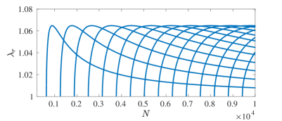
Figure 3: (Color online) MI analysis of the CW solution for $q=\omega=0.005$. In particular, real unstable Floquet multipliers, i.e., $\lambda_{r}>1$ (and $\lambda_{i}=0$) are probed as a function of the number of lattice sites $N$. The first unstable mode of CW solutions appears when $N>628$, and more and more unstable modes emerge with increasing $N$.

Finally, we would like to comment on an important observation of our spectral stability analysis results. It is known from [54], that plane wave solutions (CW) to the focusing DNLS model are modulationally unstable (a stability calculation of CW solutions to the Salerno model that contains the AL is presented in [46] too). The KM breathers (alongside with P and AB ones) are mounted atop a finite yet modulationally unstable background (per the focusing DNLS and AL) where localized solutions may perturb the CW Floquet spectrum. In light of the spectral stability analysis results of Fig. 2(b) and the discretization used in the present calculation, remarkably, no unstable modes are observed other than the weakly unstable one mentioned previously. We also note that the time-translation mode $1+0\mathrm{i}$ is accurately resolved in our computations.

We investigated the absence of instabilities of the KM breather of Fig. 2(a) by performing a modulational instability (MI) analysis of the CW with $q=\omega_{b}=0.005$ parametrically as a function of the number of sites $N$. Our respective results are shown in Fig. 3 where we probe the real unstable modes $\lambda_{r}$ as a function of $N$. In conjuction with the spectrum of Fig. 2(b) with $N=600$, the MI analysis for the same $N$, surprisingly does not predict the presence of CW unstable modes. In fact, this is true for all $N\lesssim 628$. However, for a value of $N$ just above $N=628$, we observe the emergence of the first unstable mode, and in general, the number of unstable modes starts getting increased with $N$ [cf. Fig. 3], i.e., we obtain a band of unstable modes as we approach the infinite lattice. This finding in turn suggests that for solutions sitting atop a finite yet small background, the computation of their Floquet spectrum requires the use of a very large number of sites for resolving it well.  Despite the absence of a band of real unstable modes in the Floquet spectrum of the KM breather of Fig. 2(b) and in the spectra presented next, this observation indicates that the KM solutions that we identify in this work are expected to be MI unstable as $N$ increases.

Having presented our preliminary numerical results to motivate the notion of proximity between the AL and DNLS models for small enough data, we analytically explore this proximity in the next section.

4 Theoretical justification of the proximal KM dynamics by DNLS

4.1 The case of the infinite lattice

For our subsequent theoretical analysis, we will introduce notation to distinguish the AL and DNLS limits of the Salerno model of Eq. (1).  Recall that the AL model corresponds to the $g=1$ case:

$$\mathrm{i}\dot{\Psi}_{n}+C(\Delta_{d}\Psi)_{n}+\left(\Psi_{n+1}+\Psi_{n-1}\right)|\Psi_{n}|^{2}=0,$$ (8)

whereas the DNLS model to the $g=0$ case:

$$\mathrm{i}\dot{\Phi}_{n}+C(\Delta_{d}\Phi)_{n}+2|\Phi_{n}|^{2}\Phi_{n}=0,$$ (9)

that is, $\Psi$ and $\Phi$ will stand for the solutions to the AL and DNLS models, respectively. Motivated by [52], the systems will be supplemented with general non-zero boundary conditions of the form

$$\lim_{|n|\rightarrow\infty}\Psi_{n}(t)=\lim_{|n|\rightarrow\infty}e^{2iq^{2}t}q_{n},\quad\lim_{|n|\rightarrow\infty}\Phi_{n}(t)=\lim_{|n|\rightarrow\infty}e^{2iq^{2}t}q_{n},\quad t\geq 0,$$ (10)

where

$$q_{n}=\left\{\begin{array}[]{ll}q_{-},&n\leq 0,\\ q_{+},&n>0,\end{array}\right.$$ (11)

and $q_{\pm}$ are complex constants with $|q_{\pm}|=q$. The boundary conditions of Eqs. (10)-(11) can be transformed to be time independent via the change of variables

$$\Psi_{n}(t)=e^{2iq^{2}t}\psi_{n}(t),\quad\Phi_{n}(t)=e^{2iq^{2}t}\phi_{n}(t).$$ (12)

Using the change of variables in Eq. (12), we can rewrite Eqs. (8) and (9) in the form

$$i\dot{\psi}_{n}+C(\Delta_{d}\psi)_{n}-2q^{2}\psi_{n}+|\psi_{n}|^{2}\left(\psi_{n+1}+\psi_{n-1}\right)=0,\quad$$ (13)

$$i\dot{\phi}_{n}+C(\Delta_{d}\phi)_{n}+2\left[|\phi_{n}|^{2}-q^{2}\right]\phi_{n}=0.$$ (14)

Note that the initial conditions remain unchanged under the change of variables of Eq. (12), namely, $\psi_{n}(0)=\Psi_{n}(0)$ and $\phi_{n}(0)=\Phi_{n,0}$. The boundary conditions become

$$\lim_{n\to\pm\infty}\psi_{n}(t)=\lim_{n\to\pm\infty}\phi_{n}(t)=q_{\pm},$$ (15)

so that $\displaystyle{\lim_{|n|\rightarrow\infty}|\psi_{n}(t)|=\lim_{|n|\rightarrow\infty}|\Phi_{n}(t)|=q>0}$. Next, we perform a second change of variables,

$$\psi_{n}(t)=U_{n}(t)+q_{n},\quad\phi_{n}(t)=V_{n}(t)+q_{n},$$ (16)

and Eqs. (13)-(14) become

$$i\dot{U}_{n}+C(\Delta_{d}U)_{n} +C(\Delta_{d}q)_{n}-2q^{2}(U_{n}+q_{n})$$

$$+|U_{n}+q_{n}|^{2}\left(U_{n+1}+U_{n-1}+q_{n+1}+q_{n-1}\right)=0,$$ (17)

$$i\dot{V}_{n}+C(\Delta_{d}V)_{n} +C(\Delta_{d}q)_{n}+2\left[|V_{n}+q_{n}|^{2}-q^{2}\right](V_{n}+q_{n})=0.$$ (18)

The initial conditions for the equations (4.1)-(18), become

$$U_{n}(0)=\psi_{n}(0)-q_{n},\quad V_{n}(0)=\phi_{n}(0)-q_{n},$$ (19)

and the boundary conditions are zero at infinity, i.e.,

$$\lim_{n\rightarrow\pm\infty}U_{n}(t)=\lim_{n\rightarrow\pm\infty}V_{n}(t)=0,\quad t\geq 0.$$ (20)

Along the lines of [55] (see also [52] for the continuous counterpart), we can prove that, for any initial conditions $U(0),V(0)\in\ell^{2}$, there exist $T_{AL}^{*}(U(0)),T_{DNLS}^{*}(V(0))>0$ such that the above Cauchy problems for the modified AL and DNLS equations (4.1) and (18) have unique solutions $U\in C^{1}([0,T_{AL}^{*}(U(0))],\ell^{2})$ and $V\in C^{1}([0,T_{DNLS}^{*}(V(0))],\ell^{2})$. Starting from this local existence result and following the methods of [44, 45, 52], we can further prove that these solutions stay close to one another in the following sense:

Theorem 4.1.

Consider the Cauchy problems for the modified AL and DNLS equations (4.1) and (18) when supplemented with the initial conditions (19) and the vanishing boundary conditions at infinity (20). Let any $0<\varepsilon<1$ and assume that the initial conditions $U(0)$ and $V(0)$ have $\ell^{2}$-norms of $\mathcal{O}(\varepsilon)$, the $\ell^{2}$-distance $||U(0)-V(0)||_{\ell^{2}}$ between them is of $\mathcal{O}(\varepsilon^{3})$, and that the background amplitude $q$ is of $\mathcal{O}(\varepsilon)$, namely there exist constants $C_{i},\;i=1,...,4$

$$||U(0)||_{\ell^{2}}\leq C_{1}\varepsilon,\;\;||V(0)||_{\ell^{2}}\leq C_{2}\varepsilon,\;\;||U(0)-V(0)||_{\ell^{2}}\leq C_{3}\varepsilon^{3},\;\;\mbox{and}\;\;q\leq C_{4}\varepsilon.$$ (21)

Then, there exists $T_{c}>0$ and a positive constant $C>0$ such that the $\ell^{2}$-distance between the solutions satisfies simultaneously the upper bounds

$$\begin{aligned} &||U(t)-V(t)||_{\ell^{2}}\leq C\varepsilon^{3}t,\\ &||U(t)-V(t)||_{\ell^{2}}\leq\hat{C}\varepsilon,\end{aligned}\quad\mbox{for all}\;\;0<t\leq T_{c}.$$ (22)

Theorem 4.1 is proved in A. The time $T_{c}$ in the above proximity result is obtained as follows. Since $U\in C^{1}([0,T_{AL}^{*}],\ell^{2})$, i.e., it is continuously differentiable with respect to time, the assumption (21) implies that there exists a time $\hat{T}_{AL}\in(0,T_{AL}^{*}]$ such that the size of $U(t)$ is also of $\mathcal{O}(\varepsilon)$, that is

$$||U(t)||_{\ell^{2}}\leq C_{5}\varepsilon,\;\;\mbox{for all}\;\;t\in[0,\hat{T}_{AL}]$$ (23)

for some constant $C_{5}>0$. Similarly, there is time $\hat{T}_{DNLS}\in(0,T_{DNLS}^{*}]$ such that

$$||V(t)||_{\ell^{2}}\leq C_{6}\varepsilon,\;\;\mbox{for all}\;\;t\in[0,\hat{T}_{DNLS}],$$ (24)

for some constant $C_{6}>0$. Then, the proximity time $T_{c}$ is defined as $T_{c}=\min\big{\{}\hat{T}_{AL},\hat{T}_{DNLS}\big{\}}$.

4.2 The case of periodic boundary conditions

As described in Section 3, in the numerical simulations we supplement the lattice (3) with periodic boundary conditions. This scenario bears some significant differences and is more tractable than the case of the infinite lattice discussed above, due to the conservation laws of the systems. The phase spaces for the periodic lattice are the spaces of periodic sequences with period $N$, denoted by

$${\ell}^{p}_{per}:=\Big{\{}U=(U_{n})_{n\in\mathbb{Z}}\in\mathbb{R}:\ U_{n}=U_{n+N},\ \|U\|_{\ell^{p}_{\mathrm{per}}}:=\Big{(}h\sum_{n=0}^{N-1}|U_{n}|^{p}\Big{)}^{\frac{1}{p}}<\infty\Big{\}},\ 1\leq p\leq\infty,$$

where $h$ denotes the lattice spacing. For simplicity, we set $h=1$ (as in the numerical study which corresponds to the choice $C=\frac{1}{h^{2}}=1$ made above). In particular, we have the following analogue of Theorem 4.1, which can be proved in exactly the same way as the results given in [44, 45].

Theorem 4.2.

Consider the Cauchy problems for equations (13) and (14) when supplemented with periodic boundary conditions. Let any $0<\varepsilon<1$ and assume that the initial conditions $\psi(0)$ and $\phi(0)$ have $\ell^{2}_{per}$-norms of $\mathcal{O}(\varepsilon)$, the $\ell^{2}_{per}$-distance $||\psi(0)-\phi(0)||_{\ell^{2}_{per}}$ between them is of $\mathcal{O}(\varepsilon^{3})$, and the background amplitude $q$ is of $\mathcal{O}(\varepsilon)$, i.e. there exist positive constants $C_{i}$, $i=1,...,4$ such that

$$||\psi(0)||_{\ell^{2}_{per}}\leq C_{1}\varepsilon,\;\;||\phi(0)||_{\ell^{2}_{per}}\leq C_{2}\varepsilon,\;\;||\psi(0)-\phi(0)||_{\ell^{2}_{per}}\leq C_{3}\varepsilon^{3},\;\;\mbox{and}\;\;q\leq C_{4}\varepsilon.$$ (25)

Then, for arbitrary $0<T<\infty$, there exists a constant $\tilde{C}>0$ such that the $\ell^{2}_{per}$-distance between the solutions satisfies the estimate

$$||\psi(t)-\phi(t)||_{\ell^{2}_{per}}\leq\tilde{C}\varepsilon^{3}t,\;\;\mbox{for all}\;\;0<t\leq T.$$ (26)

The main difference between Theorems 4.1 and 4.2 is that in the latter case the conservation laws ensure the global existence of solutions, thus implying the validity of the proximity result (26) for arbitrary times.

4.3 Connection to the numerical findings of Section 3

Theorem 4.1 (for the infinite lattice with nonzero boundary conditions) and Theorem 4.2 (for the finite lattice with periodic boundary conditions) justify theoretically that the distance between the solutions of the AL and DNLS equations grows linearly at a rate which is at most of $\mathcal{O}(\varepsilon^{3})$ when the initial and background data are of $\mathcal{O}(\varepsilon)$.

In the case of Theorem 4.1, according to the well-posedness results of [52, 56], initial data and background of $\mathcal{O}(\varepsilon)$ guarantee that the $\ell^{2}$ norm of the solutions remains of $\mathcal{O}(\varepsilon)$ over a lifespan of $\mathcal{O}(\varepsilon^{-2})\simeq T_{c}$. However, beyond that lifespan, the solutions may not remain of $\mathcal{O}(\varepsilon)$ and, therefore, there may exist a time $T_{c}^{*}$ such that the distance of solutions may escape from the trapezoidal region delimited by the two upper bounds in (22). This scenario is portrayed by the left diagram of Fig. 4.

On the other hand, in the case of Theorem 4.2 for the periodic problem, the $\mathcal{O}(\varepsilon^{3})$ growth rate of the difference of solutions is transient. Indeed, recalling the conserved quantities (5) and (6), it was shown in [44] that

$$||\psi(t)||_{\ell^{2}_{per}}^{2}\leq\exp(P_{\mathrm{AL}}(0))-1\lesssim\varepsilon^{2},\quad\text{for all }t\geq 0,$$ (27)

and, furthermore, due to the conservation of $P_{\mathrm{DNLS}}$,

$$P_{\mathrm{DNLS}}(t)=||\phi(t)||^{2}_{\ell^{2}_{per}}=||\phi(0)||^{2}_{\ell^{2}_{per}}=P_{\mathrm{DNLS}}(0)\lesssim\varepsilon^{2},\quad\text{for all }t\geq 0.$$ (28)

Hence, by the triangle inequality,

$$||\psi(t)-\phi(t)||_{\ell^{2}_{per}}\leq||\psi(t)||_{\ell^{2}_{per}}+||\phi(t)||_{\ell^{2}_{per}}\leq\hat{C}\varepsilon,\;\;\mbox{for all $t\geq 0$},$$ (29)

where the constant $\hat{C}$ is independent of $t$. Consequently, the linear growth upper bound in the proximity estimate (26) is relevant only for times such that $\tilde{C}\varepsilon^{3}t\leq\hat{C}\varepsilon$, i.e.

$$t\leq\frac{\hat{C}}{\tilde{C}}\frac{1}{\varepsilon^{2}}=:T_{ub}.$$ (30)

That is, $T_{ub}$ defines the upper bound for the times where the linear growth of the distance between the solutions holds. For $t>T_{ub}$, the distance between the solutions should satisfy the uniform upper bound (29). This situation is illustrated in the right diagram of Fig. 4.

Under the $\mathcal{O}(\varepsilon)$ smallness conditions on the initial and background data (21) and (25), Theorem 4.1 for the infinite lattice supplemented with the nonzero boundary conditions (10)-(11) and Theorem 4.2 for the periodic lattice justify that the DNLS lattice admits solutions of $\mathcal{O}(\varepsilon)$ with the following properties:

1. They diverge at most linearly in time from the analytical solutions of the AL lattice in terms of the $\ell^{2}$-metric, with a linear growth rate at most of $\mathcal{O}(\varepsilon^{3})$, for finite times in $[0,T_{c}]$ in the case of the infinite lattice (left panel of Fig. 4) or satisfying at most the upper bound $T_{ub}$ given by (30) in the periodic case (right panel of Fig. 4) .

2. For all $t\geq 0$, the solutions remain close — at most of $\mathcal{O}(\varepsilon)$ with respect to the $\ell^{2}$-metric — for all $t\in[0,T_{c}]$ in the case of the infinite lattice and for all $t>0$ in the periodic case.

3. For the distance measured in all $\ell^{p}$-metrics with $p\geq 2$, due to the embedding

   $$\ell^{q}\subset\ell^{p},\quad\|u\|_{\ell^{p}}\leq\|u\|_{\ell^{q}},\quad 1\leq q\leq p\leq\infty,$$ (31)

   it is reasonable to expect an even smaller rate of proximity than the one for the $\ell^{2}$-metric for the times described above. For example, when $p=\infty$, which is relevant for a comparison of the amplitudes of solutions, it is theoretically justified to expect an improved rate of proximity.

In summary, comparing the results of Theorems 4.1 and 4.2, in the case of the infinite lattice there is a possibility that, at some finite time $T_{c}^{*}\geq T_{c}\simeq\mathcal{O}(\varepsilon^{-2})$, the distance of solutions will escape from the trapezoidal region capped by the $\mathcal{O}(\varepsilon)$ dashed horizontal line (see Fig. 4). This is due to the fact that, in the case of nonzero boundary conditions, it is not known whether the solutions are uniformly bounded. On the other hand, in the case of periodic boundary conditions, the solutions individually remain bounded by the initial data of size $\mathcal{O}(\varepsilon)$ due to the conservation of $P_{\text{DNLS}}$ and $P_{\text{AL}}$; therefore, by the triangle inequality, the distance of solutions is guaranteed to remain within the trapezoidal region below the $\mathcal{O}(\varepsilon)$ dashed horizontal line at all times (see Fig. 4).

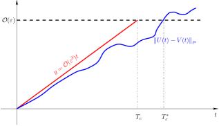
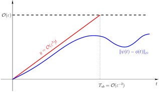
Figure 4: The behavior of the distance according to the theoretical upper bounds of Theorems 4.1-4.2. Left: The case of nonzero boundary conditions. Here, the distance of solutions may increase beyond $\mathcal{O}(\varepsilon)$ at finite time. Right: The case of periodic boundary conditions. Here, according to the uniform bound of inequality (29), the distance of solutions is at most $\mathcal{O}(\varepsilon)$ for all times. It should be noted that, in certain scenarios, the distance curve (in blue) may be much closer to the $t$-axis than what is depicted above, at least for an initial time interval — e.g. see the corresponding graphs of Fig. 5.

It is remarkable that the numerical findings of Section 3 for the case of the KM solutions showcase that the growth rate of the distance is significantly lower than the ones associated with the theoretical bounds, and the order of proximity is much higher than what is predicted theoretically. This is in accordance with several numerical findings for both discrete [44, 45] and continuous [52] setups, which illustrate that the rate of divergence and proximity may depend on the particular analytical solution of the integrable system considered. In many cases (bright solitons [44], fast soliton collisions [52]), this rate is of $\mathcal{O}(\varepsilon^{p})$ with $p>3$. Indicatively, and in line with the numerical study of Fig. 1, the rate of divergence of the solutions was found to be in the neighborhood of $\varepsilon^{5}$.

\begin{overpic}[height=80.94424pt,angle={0}]{fig5a.pdf} \put(18.0,60.0){{\small(a)}} \end{overpic}

\begin{overpic}[height=80.94424pt,angle={0}]{fig5b.pdf} \put(18.0,60.0){{\small(b)}} \end{overpic}

\begin{overpic}[height=80.94424pt,angle={0}]{fig5c.pdf} \put(80.0,35.0){{\small(c)}} \end{overpic}

\begin{overpic}[height=80.94424pt,angle={0}]{fig6a.pdf} \put(18.0,60.0){{\small(d)}} \end{overpic}

\begin{overpic}[height=80.94424pt,angle={0}]{fig6b.pdf} \put(18.0,60.0){{\small(e)}} \end{overpic}

\begin{overpic}[height=80.94424pt,angle={0}]{fig6c.pdf} \put(80.0,35.0){{\small(f)}} \end{overpic}

Figure 5: Summary of numerical results for the AL and DNLS models [cf. Eqs. (13) and (14)] in conjuction with our theoretical analysis on their proximity. We evolve KM initial data with $(q,\omega_{b},\varepsilon)\simeq(0.09,0.01,0.054)$ and $(q,\omega_{b},\varepsilon)\simeq(0.34,0.46,0.425)$ in the top and bottom rows, respectively, over two periods. Panels (a) and (d), and (b) and (e) depict the spatio-temporal evolution of the amplitudes $|\psi_{n}|$ and $|\phi_{n}|$, respectively. The panels (c) and (f) summarize the comparisons made between the theoretical estimates on the proximity of the models with the numerically obtained distance (see, the legend and insets therein) of the solutions after subtracting the background $q$ (see, text for details).

We conclude our theoretical analysis by showcasing two examples comparing the theoretical estimates with the numerical computations of Fig. 5. Note that, for computational purposes, we may consider the assumptions (21) with constants $C_{i}=1$, $i=1,...,4$. Then, we may consider the relevant times $\hat{T}_{AL},~\hat{T}_{DNLS}$ such that the bounds (23) and (24) hold with the constants $C_{5}=C_{6}=1$. For this choice of unit constants $C_{i}$, we may derive an explicit form of the closeness estimate (22) by inserting the estimates (23) and (24) in (43) and (44), respectively. This way, by using (47), we derive the following explicit form of the bound (22) depending on $\varepsilon$ and $q$,

$$||U(t)-V(t)||_{\ell^{2}}\leq\alpha t,\;\;\alpha=3\varepsilon^{3}+9q\varepsilon^{2}+12q^{2}\varepsilon.$$ (32)

The top and bottom rows of Fig. 5 correspond to the cases with $(q,\omega_{b})=(0.09,0.01)$ and $(0.34,0.46)$, respectively. Same as before, we employ a lattice of $N=600$ sites, and use the exact KM solution of Eq. (4) as an initial condition for both the AL and DNLS models. The panels (a) and (d), and (b) and (e) showcase the spatio-temporal evolution of the amplitude of the KM solution (in the respective cases) for the AL and DNLS models, respectively, over 2 periods. In line with Fig. 4, we summarize our proximity results in panels (c) and (f) of Fig. 5 where the solid blue line (see the legend in panel (c)) shows the distance of the solutions in the $l^{2}$ norm after removing the background $q$. The horizontal dashed black line corresponds to $y=2\|U(0)\|_{l^{2}}=2\varepsilon$, whereas the solid red line to $y=\alpha t$, with $\alpha$ given by (32). For panels (a)-(c), $\varepsilon\simeq 0.054$, while for panels (d)-(f) we used $\varepsilon\simeq 0.425$. Recall that, according to the theoretical results of Theorem 4.1 and 4.2, the solutions should remain proximal for minimal guaranteed times of $T_{c}\simeq\mathcal{O}(\varepsilon^{-2})$. The numerical results of Figs. 5(c) and (f) confirm this fact, since they show that the two models are proximal up to times $\approx 512$ (top row) and $\approx 5.86$ (bottom row), see the insets therein. Furthermore, the comparison of the patterns over the proximity time scales justify accordingly the proximity of the spatiotemporal dynamics manifested by the emergence of the first apparent localization event in each of the panel pairs (a)-(b) and (d)-(e), respectively. Beyond this time, the MI effects manifest themselves in the evolution of the KM for the DNLS model (see, panels (b) and (e)), along the lines of the results of [57]. Those effects contribute to the increase of the distance between the solutions of the AL and DNLS models, although the latter always remains bounded by the linear, theoretically predicted growth of Figs. 5(c) and (f); see the respective red lines. It is also interesting to observe that while the blue line of the numerically observed difference starts growing, due to the development of the modulational instability in panels (b) and (e), i.e., for the DNLS model, its growth appears to be almost the same as the analytical growth rate $\alpha$ of the linear upper bound of Eq. (32) (while of course resting well below the rigorously established bound of the red line). Lastly, when the instability growth, seeded at the location of the localized (in space-time) solution reaches the domain boundary, we observe the relative difference between the two model solutions (AL and DNLS) saturating, with the blue line becoming nearly horizontal. The above analysis provides a theoretical justification of the strategy followed in Section 3, namely of inserting the analytical KM solution with the prescribed set of parameters as an initial guess for the Newton’s method which resulted in finding the solution shown in Fig. 2.

5 Branches of Numerically-Exact KM-type breather solutions to the DNLS

The numerical results of Sec. 3 paired with our theoretical analysis on the proximity of the DNLS and AL models now raise the question whether branches of KM-type solutions with a flat background to the DNLS model [cf. Eq. (3)] can be obtained numerically over the background amplitude $q$ and (breathing) frequency $\omega_{b}$. Unlike the earlier work of [49], where the starting point for exploration was the anti-continuum limit, here, we leverage the existence of the KM-type breather of Fig. 2 in our numerical investigations presented next.

In particular, we use the profile of Fig. 2 with $q=\omega_{b}=0.005$ (that our nonlinear solver converged to) as well as one with $q=0.005$ and $\omega_{b}=0.01$ as initial guesses to a pseudo-arclength continuation method [58], and trace branches of KM-type breathers over the background amplitude $q$. In our computations presented in this section, we employ a lattice with $N=200$ sites, and periodic boundary conditions are imposed at the edges of the lattice while keeping the same number of Fourier modes in time the same as before, i.e., $k=41$, and thus $2k+1=83$. At each continuation step, we identify the spectral stability of the solutions by computing the Floquet multipliers of the associated monodromy matrix, and the stability traits of the solutions are corroborated by performing direct numerical simulations of select profiles through the use of MATLAB’s built-in ode113 integrator.

We turn now our focus to the numerical results that are summarized in Figs. 6 and 7 corresponding to KM-type branches to the DNLS with $\omega_{b}=0.005$ and $\omega_{b}=0.01$, respectively. The top panels in the figures showcase the dependence of the $l^{2}$ norm of the solution on $q$, and the labels therein connect with the panels that follow below. In particular, the left i.e., (a)-(c) and middle (d)-(f) panels in the figures, depict the spatial distribution of the amplitude of the solutions, i.e., $|\psi_{n}|$ and their Floquet multipliers (shown with red markers) on the spectral plane, respectively, for different values of $q$ along the respective branches (see, the captions in the figures for the specific values of $q$). The panels (g)-(i) present the spatio-temporal evolution of the profiles of panels (a)-(c) over 20 periods, i.e., $20\times T_{b}$ where $T_{b}\approx 2.5133\times 10^{4}$ and $T_{b}\approx 628.3185$ in Figs. 6 and 7, respectively.

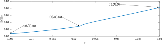
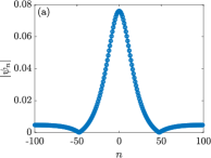
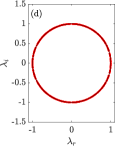
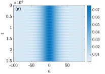
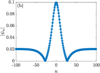
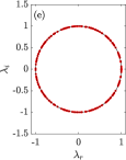
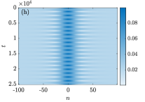
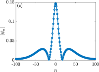
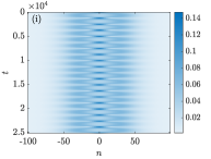
Figure 6: (Color online) Bifurcation analysis results of KM breathers to the DNLS equation over background amplitude $q$, and for fixed $\omega_{b}=0.005$. Panels (a)-(c) show numerically exact solution profiles corresponding to values of $q=0.005$, $q=0.0214$, and $q=0.0400$, respectively. Panels (d)-(f) give the corresponding Floquet multipliers, i.e., the eigenvalues of the associated monodromy matrix. Finally, the panels (g)-(i) show the dynamical evolution of the KM solutions shown in panels (a)-(c) over time, up to $20$ periods. A switch in the phenomenology of the solutions occurs beyond $q=0.0214$, where solutions no longer sit atop a constant background (see, panel (c)).

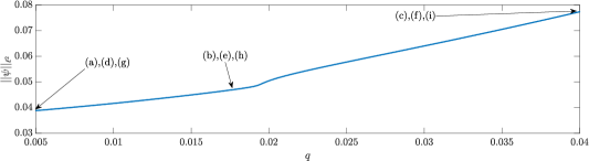
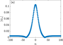
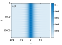
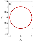
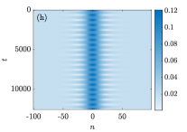
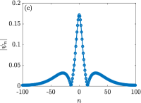
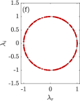
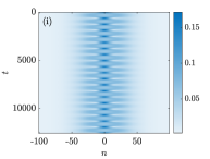
Figure 7: (Color online) Same Fig. 6 but for $\omega_{b}=0.01$. Panels (a)-(c) show numerically exact solution profiles corresponding to values of $q=0.005$, $q=0.0176$, and $q=0.0400$, respectively. Panels (d)-(f) showcase the corresponding Floquet multipliers of these solutions. Panels (g)-(i) show the dynamical evolution of the KM solutions shown in panels (a)-(c) over time, (again) up to $20$ periods. A switch in the phenomenology of the solutions occurs beyond $q=0.0176$, where solutions no longer sit atop a constant background.

Starting from $q=0.005$, it can be discerned from the bifurcation diagram of Fig. 6 (corresponding to $\omega_{b}=0.005$) that a branch of KM-type solutions sitting atop a constant background does exist up until $q\approx 0.0214$, see, the profiles of panels (a) and (b), respectively, where a “blip” occurs that highlights the manifestation of the change in the characteristics of the solutions. Past that value of $q$, the solutions feature same characteristics as the KM breather of Eq. (4) but only locally, that is, the solutions bear a peak maximum surrounded by two minima (of zero amplitude) although the spatial asymptotics are different. Indeed, this is evident in Fig. 6(c) corresponding to $q=0.04$ where the tails of the solution’s amplitude gradually asymptote to zero for $|n|\gg 1$. A similar phenomenology is observed for the numerical results of Fig. 7 corresponding to $\omega_{b}=0.01$. Upon tracing the relevant branch from $q=0.005$, the bifurcation diagram indicates the existence of a branch of KM-type solutions atop a flat background up to $q\approx 0.0176$ whereupon for larger values of $q$, the tails of the solution (again) asymptote to zero. This change in the characteristics of the asymptotics of the solution is imprinted by the presence of a blip in the bifurcation diagram shown in the top panel of Fig. 7.

As far as the stability analysis results are concerned, the Floquet spectra of panels (d)-(f) of Figs. 6 and 7 indicate that the KM solutions to the DNLS that we report are spectrally stable via the absence of multipliers that lie off the unit circle (the latter shown with a solid black line in the panels), i.e., $|\lambda|>1$, for the number of lattice nodes we used.  In line with the earlier comment made in Sec. 3, however, all these solutions are typically expected to be MI unstable as $N$ starts getting increased, see, Fig. 3. Regardless, and for the discretization we used herein, we report (after careful inspection of the multipliers) the emergence of just one real eigenvalue with $|\lambda|-1=\mathcal{O}(10^{-5})$ (or $\mathcal{O}(10^{-6})$) in each case we studied with a positive real part (data not shown), a (weakly unstable) case that is strongly reminiscent of the results of Fig. 2.

Similar to Fig. 2(c), we checked the robustness of the solutions of panels (a)-(c) of Figs. 6 and 7 by evolving them forward in time. The spatio-temporal dynamics shown in panels (g)-(i) give strong evidence that the solutions breathe in time, and are indeed robust over 20 periods (note the large terminal times of integration, which are of order of $\mathcal{O}(10^{4})$). As a further check, we performed dynamics of the DNLS by using perturbed versions of the KM solutions along the most unstable eigendirection (with a very small yet positive real part) we identified in this work as initial conditions, and monitored the breathing dynamics over $1000$ periods. Remarkably, all the KM-type solutions that we have identified in this work and per the number of lattice sites used are dynamically robust (data not shown). However, it is expected that as $N$ increases, the emergence of MI modes (see Fig. 3) will leave an imprint in the aforementioned KM’s Floquet spectra which itself may affect the dynamics of the KM breathers, depending on the growth rates of such unstable modes.

Based on the above results, we conclude that for sufficiently small amplitudes of the background, solutions with features very proximal to those to the AL model, that are for practical purposes very long-lived can be found in the DNLS model (for large lattices). As the value of the background increases, the solutions change character past a “critical point” (as was shown through computations for two different frequencies), leading to waveforms that may locally resemble the KMs of the AL model but do not share the same asymptotic behavior. Once again, it appears that the smallness of the data is central to obtaining proximal results in the form of genuine time-periodic solutions across the DNLS and AL model. It remains an important open question whether such solutions can be generalized to arbitrary amplitudes in some suitable form in the DNLS case.

6 Conclusions and Future Challenges

In the present work we explore the proximity of the DNLS and the AL model, i.e., of the non-integrable and integrable discretizations of the nonlinear Schrödinger equation. In particular, our investigation focuses on waveforms that are time-periodic in the form of Kuznetsov-Ma solitons and exist atop a finite background. These structures are of particular interest due to their connection with the rogue wave nonlinear patterns. We illustrated herein that suitable conditions (of background, frequency, etc.) can be identified under which the DNLS and AL solutions can barely be distinguished for long simulations in time. This, in turn, motivated us to explore this proximity analytically, whereby we found that the distance between the models grows only linearly in time with a suitable prefactor depending on the size and distance between the initial conditions in the two models. Finally, we systematically analyzed such waveforms and nonlinear dynamics at the level of the DNLS (and AL) models, identifying them as exact periodic solutions and performing suitable continuations.

Naturally, this study paves the way for further explorations along this vein. While we have used periodic orbits herein due to the ability to identify them in a numerically exact form (up to prescribed tolerance), it would be relevant to appreciate and formulate similar results for other states, including Peregrine solitons, Akhmediev breathers, as well as for higher order rogue waveforms. Our examination also took place at the level of the discrete models, without seeking to examine the relevant results as a function of the discretization parameter and how the corresponding (shared) continuum limit of the models is approached. The latter point is also worthy of further exploration. Finally, we restricted our considerations to the case of focusing DNLS and AL models. However, it is remarkable that in the case of the discrete models such rogue patterns may arise in defocusing variants of the models as well [59], as well as the very recent work of [60]. The latter settings are also of considerable interest at the level of the considerations presented herein. Such studies are currently under progress and will be reported in future publications.

Appendix A Proof of Theorem 4.1

First, it is important to discuss some properties of the nonlinear operators appearing in equations (4.1) and (18). For the equation (4.1), we consider the nonlinear operator

$$\mathcal{G}_{AL}(U_{n})=C(\Delta_{d}U)_{n}+C(\Delta_{d}q)_{n}+\mathcal{F}_{AL}(U_{n}),$$ (33)

where

$$\mathcal{F}_{AL}(U_{n})=-2q^{2}(U_{n}+q_{n})+|U_{n}+q_{n}|^{2}\left(U_{n+1}+U_{n-1}+q_{n+1}+q_{n-1}\right).$$

The operator $\mathcal{F}_{AL}(U_{n})$ can be rewritten in the form,

$$\mathcal{F}_{AL}(U_{n})=-2q^{2}U_{n} - 2q^{2}q_{n}+\left(|U_{n}|^{2}+\overline{q}_{n}U_{n}+q_{n}\overline{U}_{n}\right)\left(U_{n+1}+U_{n-1}+q_{n+1}+q_{n-1}\right)$$ (34)

$$+ |q_{n}|^{2}\left(U_{n+1}+U_{n-1}\right)+|q_{n}|^{2}\left(q_{n+1}+q_{n-1}\right).$$

The operator $\mathcal{G}_{AL}$ given in (33) will be well defined on bounded sets of $\ell^{2}$, if and only if

$$(\Delta_{d}q)_{n}=0\;\;\mbox{or}\;\;(\Delta_{d}q)_{n}\in\ell^{2},$$ (35)

due to the presence of the second term of $\mathcal{G}_{AL}$, and

$$-2q^{2}q_{n}+|q_{n}|^{2}\left(q_{n+1}+q_{n-1}\right)=0\;\;\mbox{or}\;\;-2q^{2}q_{n}+|q_{n}|^{2}\left(q_{n+1}+q_{n-1}\right)\in\ell^{2},$$ (36)

due to the presence of the second and the last term of $\mathcal{F}_{AL}$ in (34). By the definition of $q_{n}$ in (11), we have $|q_{n}|^{2}=q^{2}$ and, thus, condition (36) coincides with condition (35).

Both options of (35) are valid: if $\zeta_{+}=\zeta_{-}$, then $(\Delta_{d}q)_{n}=0$. If $\zeta_{+}\neq\zeta_{-}$, then $(\Delta_{d}q)_{n}=(\zeta_{+}-\zeta_{-})(\delta_{n}-\delta_{n-1})$, where $\delta_{n}$ is the discrete $\delta$-function, and obviously $(\Delta_{d}q)_{n}\in\ell^{2}$.

For the equation (18), we consider the operator

$$\mathcal{G}_{DNLS}(V_{n})=C(\Delta_{d}V)_{n}+C(\Delta_{d}q)_{n}+\mathcal{F}_{DNLS}(V_{n}),$$ (37)

where

$$\mathcal{F}_{DNLS}(V_{n})=+2\left[|V_{n}+q_{n}|^{2}-q^{2}\right](V_{n}+q_{n}).$$

After some algebra, $\mathcal{F}_{DNLS}(V_{n})$ is rewritten in the form

$$\mathcal{F}_{DNLS}(V_{n})=|V_{n}|^{2}V_{n}+2q_{n}|V_{n}|^{2}+2|q_{n}|^{2}V_{n}+\overline{q}_{n}V_{n}^{2}+q_{n}^{2}\overline{V}_{n}-q^{2}V_{n}+|q_{n}|^{2}q_{n}-q^{2}q_{n}.$$ (38)

Since $|q_{n}|^{2}=q^{2}$, we have

$$|q_{n}|^{2}q_{n}-q^{2}q_{n}=0.$$

Moreover, for the second term of the operator $\mathcal{G}_{DNLS}$, the condition (35) is satisfied as explained above.

Next, we consider the difference of solutions $D(t):=U(t)-V(t)$, of the initial-boundary value problems (4.1) and (18) supplemented with the zero boundary (20), respectively. Subtracting equation (18) from equation (4.1), we see that $D(t)$ satisfies the equation

$$i\dot{D_{n}}+C(\Delta_{d}D)_{n}=\mathcal{F}_{DNLS}(V_{n})-\mathcal{F}_{AL}(U_{n}).$$ (39)

Multiplying (39) by $\overline{{D}_{n}}$, summing over $n$ and keeping the imaginary parts of the resulting equation, we get that $||D(t)||_{\ell^{2}}$ satisfies the inequality

$$\frac{1}{2}\frac{d}{dt}||D||_{\ell^{2}}^{2} = \sum_{n\in\mathbb{Z}}\mathcal{F}_{DNLS}(V_{n})\overline{{D}_{n}}-\sum_{n\in\mathbb{Z}}\mathcal{F}_{AL}(U_{n})\overline{{D}_{n}}$$ (40)

$$\leq ||\mathcal{F}_{DNLS}(V)||_{\ell^{2}}||D||_{\ell^{2}}+||\mathcal{F}_{AL}(U)||_{\ell^{2}}||D||_{\ell^{2}}.$$

Since $\frac{1}{2}\frac{d}{dt}||D||_{\ell^{2}}^{2}=||D||_{\ell^{2}}\frac{d}{dt}||D||_{\ell^{2}}$, after an integration with respect to time, inequality (40) becomes

$$||D(t)||_{\ell^{2}}\leq||D(0)||_{\ell^{2}}+\int_{0}^{t}||\mathcal{F}_{AL}(U(s))||_{\ell^{2}}ds+\int_{0}^{t}||\mathcal{F}_{DNLS}(U(s))||_{\ell^{2}}ds.\;\;\;\;$$ (41)

Next, we shall use the following estimates: For $||\mathcal{G}_{AL}(U(s))||_{\ell^{2}}$, by using the embedding

$$\ell^{q}\subset\ell^{p},\quad\|u\|_{\ell^{p}}\leq\|u\|_{\ell^{q}},\quad 1\leq q\leq p\leq\infty,$$ (42)

for $p=4,6$ and $q=2$, we have

$$||\mathcal{F}_{AL}(U)||_{\ell^{2}} \leq \left(\sum_{n\in\mathbb{Z}}|U_{n}|^{4}|U_{n+1}+U_{n-1}|^{2}\right)^{\frac{1}{2}}+2\left(\sum_{n\in\mathbb{Z}}|q_{n}|^{2}|U_{n}|^{2}|U_{n+1}+U_{n-1}|^{2}\right)^{\frac{1}{2}}$$ (43)

$$+\left(\sum_{n\in\mathbb{Z}}|U_{n}|^{4}|q_{n+1}+q_{n-1}|^{2}\right)^{\frac{1}{2}}+2\left(\sum_{n\in\mathbb{Z}}|q_{n}|^{2}|U_{n}|^{2}|q_{n+1}+q_{n-1}|^{2}\right)^{\frac{1}{2}}$$

$$+\left(\sum_{n\in\mathbb{Z}}|q_{n}|^{4}|U_{n+1}+U_{n-1}|^{2}\right)^{\frac{1}{2}}+2q^{2}\left(\sum_{n\in\mathbb{Z}}|U_{n}|^{2}\right)^{\frac{1}{2}}$$

$$\leq 2||U(t)||_{\ell^{6}}^{3}+6q||U(t)||^{2}_{\ell^{4}}+8q^{2}||U(t)||_{\ell^{2}}$$

$$\leq 2||U(t)||_{\ell^{2}}^{3}+6q||U(t)||^{2}_{\ell^{2}}+8q^{2}||U(t)||_{\ell^{2}}.$$

Similarly, for $||\mathcal{G}_{DNLS}(V(s))||_{\ell^{2}}$, we have the estimate

$$||\mathcal{F}_{DNLS}(V)||_{\ell^{2}} \leq \left(\sum_{n\in\mathbb{Z}}|V_{n}|^{6}\right)^{\frac{1}{2}}+3\left(\sum_{n\in\mathbb{Z}}|q_{n}|^{2}|V_{n}|^{4}\right)^{\frac{1}{2}}$$ (44)

$$+3\left(\sum_{n\in\mathbb{Z}}|q_{n}|^{4}|V_{n}|^{2}\right)^{\frac{1}{2}}+q^{2}\left(\sum_{n\in\mathbb{Z}}|V_{n}|^{2}\right)^{\frac{1}{2}}$$

$$\leq ||V(t)||_{\ell^{6}}^{3}+3q||V(t)||^{2}_{\ell^{4}}+4q^{2}||V(t)||_{\ell^{2}}$$

$$\leq ||V(t)||_{\ell^{2}}^{3}+3q||V(t)||^{2}_{\ell^{2}}+4q^{2}||V(t)||_{\ell^{2}}.$$

Since $U\in C^{1}([0,T_{AL}^{*}(U(0))],\ell^{2})$, that is continuously differentiable with respect to time, the assumption (21) implies that there exist a time $\hat{T}_{AL}$, satisfying $0<\hat{T}_{AL}\leq T_{AL}^{*}(U(0))$, such that $||V(t)||_{\ell^{2}}$ will be also of order $\mathcal{O}(\varepsilon)$ for all $t\in[0,\hat{T}_{AL}]$, that is,

$$||U(t)||_{\ell^{2}}\leq C_{5}\varepsilon,\;\;\mbox{for all}\;\;t\in[0,\hat{T}_{AL}].$$ (45)

for some $C_{5}>0$. Also, since $V\in C^{1}([0,T_{DNLS}^{*}(U(0)),\ell^{2})$, again the assumption (21) implies that there exist a time $\hat{T}_{DNLS}$, satisfying $0<\hat{T}_{DNLS}\leq T_{DNLS}^{*}(U(0))$, such that $||V(t)||_{\ell^{2}}$ will be also of order $\mathcal{O}(\varepsilon)$ for all $t\in[0,\hat{T}_{DNLS}]$, that is,

$$||V(t)||_{\ell^{2}}\leq C_{6}\varepsilon,\;\;\mbox{for all}\;\;t\in[0,\hat{T}_{DNLS}],$$ (46)

for some constant $C_{6}>0$. We define $T_{c}=\min\left\{\hat{T}_{AL},\hat{T}_{DNLS}\right\}$. Then for all $t\in[0,T_{c}]$, we may estimate the integral terms of the formula (41), by using the estimates (45) and (46) in the common interval $[0,T_{c}]$ for which they are both valid. This procedure will lead to the following estimate for the distance between the solutions $U(t)$ and $V(t)$

$$||U(t)-V(t)||_{\ell^{2}} \leq C_{3}\varepsilon^{3}t+C_{7}(q\varepsilon^{2}+q^{2}\varepsilon)t,$$ (47)

where $C_{7}$ is a positive constant depending on $C_{5}$ and $C_{6}$. Inserting the assumption (21) on $q$, we derive the first of the estimates (22) with the constant $C$ depending on $C_{3}$ and $C_{7}$.

The second estimate of (22) is a consequence of the triangle inequality. Indeed, by using (45) and (46), we get

$$||U(t)-V(t)||_{\ell^{2}} \leq ||U(t)||_{\ell^{2}}+||V(t)||_{\ell^{2}}\leq\hat{C}\varepsilon,\;\;\hat{C}=C_{5}+C_{6},$$

which is the second of the estimates given in (22).

References

- Aubry [2006] S. Aubry, Physica D 216, 1 (2006).
- Flach and Gorbach [2008] S. Flach and A. V. Gorbach, Physics Reports 467, 1 (2008).
- Lederer et al. [2008] F. Lederer, G. I. Stegeman, D. N. Christodoulides, G. Assanto, M. Segev, and Y. Silberberg, Physics Reports 463, 1 (2008).
- Morsch and Oberthaler [2006] O. Morsch and M. Oberthaler, Rev. Mod. Phys. 78, 179 (2006).
- Remoissenet [1999] M. Remoissenet, Waves Called Solitons (Springer-Verlag, Berlin, 1999).
- Nesterenko [2001] V. Nesterenko, Dynamics of Heterogeneous Materials (Springer-Verlag, New York, 2001).
- Starosvetsky et al. [2017] Y. Starosvetsky, K. Jayaprakash, M. A. Hasan, and A. Vakakis, Dynamics and Acoustics of Ordered Granular Media (World Scientific, Singapore, 2017).
- Chong and Kevrekidis [2018] C. Chong and P. G. Kevrekidis, Coherent Structures in Granular Crystals: From Experiment and Modelling to Computation and Mathematical Analysis, 1st ed. (Springer International Publishing, 2018).
- Binder et al. [2000] P. Binder, D. Abraimov, A. V. Ustinov, S. Flach, and Y. Zolotaryuk, Phys. Rev. Lett. 84, 745 (2000).
- Trías et al. [2000] E. Trías, J. J. Mazo, and T. P. Orlando, Phys. Rev. Lett. 84, 741 (2000).
- Sato et al. [2006] M. Sato, B. E. Hubbard, and A. J. Sievers, Rev. Mod. Phys. 78, 137 (2006).
- Peyrard and Bishop [1989] M. Peyrard and A. R. Bishop, Phys. Rev. Lett. 62, 2755 (1989).
- Kevrekidis [2011] P. G. Kevrekidis, IMA Journal of Applied Mathematics 76, 389 (2011), https://academic.oup.com/imamat/article-pdf/76/3/389/2257051/hxr015.pdf .
- Gallavotti [2008] G. Gallavotti, The Fermi–Pasta–Ulam Problem: A Status Report (Springer-Verlag, Berlin, Germany, 2008).
- Kevrekidis [2009] P. G. Kevrekidis, The discrete nonlinear Schrödinger Equation, 1st ed. (Springer-Verlag, Heidelberg, 2009).
- Eilbeck and Johansson [2003] J. C. Eilbeck and M. Johansson, Localization and Energy Transfer in Nonlinear Systems , pp. 44 (2003).
- Ablowitz and Cole [2022] M. J. Ablowitz and J. T. Cole, Physica D: Nonlinear Phenomena 440, 133440 (2022).
- Leykam et al. [2018] D. Leykam, A. Andreanov, and S. Flach, Adv. Phys.: X 3, 1473052 (2018).
- Danieli et al. [2024] C. Danieli, A. Andreanov, D. Leykam, and S. Flach, Nanophotonics 13, 3925 (2024).
- Ablowitz et al. [2004] M. Ablowitz, B. Prinari, and A. Trubatch, Discrete and Continuous Nonlinear Schrödinger Systems (Cambridge University Press, Cambridge, 2004).
- Salerno [1992] M. Salerno, Physical Review A 46, 6856 (1992).
- Kharif et al. [2009] C. Kharif, E. Pelinovsky, and A. Slunyaev, Rogue Waves in the Ocean, Advances in Geophysical and Environmental Mechanics and Mathematics (Springer-Verlag, Berlin Heidelberg, 2009).
- Kibler et al. [2010] B. Kibler, J. Fatome, C. Finot, G. Millot, F. Dias, G. Genty, N. Akhmediev, and J. M. Dudley, Nature Phys 6, 790 (2010).
- Kibler et al. [2012] B. Kibler, J. Fatome, C. Finot, G. Millot, G. Genty, B. Wetzel, N. Akhmediev, F. Dias, and J. M. Dudley, Sci. Rep. 2, 463 (2012).
- DeVore et al. [2013] P. T. S. DeVore, D. R. Solli, D. Borlaug, C. Ropers, and B. Jalali, J. Opt. 15, 064001 (2013).
- Frisquet et al. [2016] B. Frisquet, B. Kibler, P. Morin, F. Baronio, M. Conforti, G. Millot, and S. Wabnitz, Sci Rep 6, 20785 (2016).
- Chabchoub et al. [2011] A. Chabchoub, N. P. Hoffmann, and N. Akhmediev, Phys. Rev. Lett. 106, 204502 (2011).
- Chabchoub et al. [2012] A. Chabchoub, N. Hoffmann, M. Onorato, and N. Akhmediev, Phys. Rev. X 2, 011015 (2012).
- Chabchoub and Fink [2014] A. Chabchoub and M. Fink, Phys. Rev. Lett. 112, 124101 (2014).
- Bailung et al. [2011] H. Bailung, S. K. Sharma, and Y. Nakamura, Phys. Rev. Lett. 107, 255005 (2011).
- Romero-Ros et al. [2024] A. Romero-Ros, G. C. Katsimiga, S. I. Mistakidis, S. Mossman, G. Biondini, P. Schmelcher, P. Engels, and P. G. Kevrekidis, Phys. Rev. Lett. 132, 033402 (2024).
- Yan [2012] Z. Yan, J. Phys.: Conf. Ser. 400, 012084 (2012).
- Onorato et al. [2013] M. Onorato, S. Residori, U. Bortolozzo, A. Montina, and F. T. Arecchi, Phys. Rep. 528, 47 (2013).
- Dudley et al. [2014] J. M. Dudley, F. Dias, M. Erkintalo, and G. Genty, Nature Photon 8, 755 (2014).
- Mihalache [2017] D. Mihalache, Rom. Rep. Phys 69, 28 (2017).
- Dudley et al. [2019] J. M. Dudley, G. Genty, A. Mussot, A. Chabchoub, and F. Dias, Nat. Rev. Phys. 1, 675 (2019).
- Ankiewicz et al. [2010] A. Ankiewicz, N. Akhmediev, and J. M. Soto-Crespo, Phys. Rev. E 82, 026602 (2010).
- Peregrine [1983] D. H. Peregrine, ANZIAM J. 25, 16 (1983).
- Akhmediev and Korneev [1986] N. N. Akhmediev and V. I. Korneev, Theor Math Phys 69, 1089 (1986).
- Kuznetsov [1977] E. A. Kuznetsov, Sov. Phys.-Dokl. 236, 575 (1977).
- Ma [1979] Y.-C. Ma, Stud. Appl. Math. 60, 43 (1979).
- Maluckov et al. [2009] A. Maluckov, L. Hadžievski, N. Lazarides, and G. P. Tsironis, Phys. Rev. E 79, 025601 (2009).
- Hoffmann et al. [2018] C. Hoffmann, E. Charalampidis, D. Frantzeskakis, and P. Kevrekidis, Physics Letters A 382, 3064 (2018).
- Hennig et al. [2022a] D. Hennig, N. I. Karachalios, and J. Cuevas-Maraver, Journal of Differential Equations 316, 346 (2022a).
- Hennig et al. [2022b] D. Hennig, N. I. Karachalios, and J. Cuevas-Maraver, Journal of Mathematical Physics 63, 042701 (2022b).
- Sullivan et al. [2020] J. Sullivan, E. Charalampidis, J. Cuevas-Maraver, P. Kevrekidis, and N. Karachalios, Eur. Phys. J. Plus 135, 607 (2020).
- Ablowitz and Ladik [1975] M. J. Ablowitz and J. F. Ladik, Journal of Mathematical Physics 16, 598 (1975), https://pubs.aip.org/aip/jmp/article-pdf/16/3/598/19098391/598_1_online.pdf .
- Ablowitz and Ladik [1976] M. J. Ablowitz and J. F. Ladik, Journal of Mathematical Physics 17, 1011 (1976), https://pubs.aip.org/aip/jmp/article-pdf/17/6/1011/19096120/1011_1_online.pdf .
- Charalampidis et al. [2024] E. Charalampidis, G. James, J. Cuevas-Maraver, D. Hennig, N. Karachalios, and P. Kevrekidis, Wave Motion 128, 103324 (2024).
- Akhmediev et al. [2009] N. Akhmediev, A. Ankiewicz, and M. Taki, Physics Letters A 373, 675 (2009).
- Hennig et al. [2022c] D. Hennig, N. I. Karachalios, and J. Cuevas-Maraver, Journal of Differential Equations 316, 346 (2022c).
- Hennig et al. [2024] D. Hennig, N. I. Karachalios, D. Mantzavinos, J. Cuevas-Maraver, and I. G. Stratis, Journal of Differential Equations 397, 106 (2024).
- Hairer et al. [1993] E. Hairer, G. Wanner, and S. P. Nørsett, Solving Ordinary Differential Equations I: Nonstiff Problems, 2nd ed. (Springer-Verlag, Heidelberg, 1993).
- Kivshar and Peyrard [1992] Y. S. Kivshar and M. Peyrard, Phys. Rev. A 46, 3198 (1992).
- Fotopoulos et al. [2024] G. Fotopoulos, N. I. Karachalios, V. Koukouloyannis, P. Kyriazopoulos, and K. Vetas, Journal of Nonlinear Science, article in press (2024).
- Hennig et al. [2025] D. Hennig, N. I. Karachalios, D. Mantzavinos, and D. Mitsotakis, Wave Motion 132, Paper No. 103419 (2025).
- Biondini et al. [2018] G. Biondini, S. Li, D. Mantzavinos, and S. Trillo, SIAM Rev. 60, 888 (2018).
- Kuznetsov [2023] Y. A. Kuznetsov, Elements of Applied Bifurcation Theory, Applied Mathematical Sciences (Springer-Verlag, New York, 2023).
- Ohta and Yang [2014] Y. Ohta and J. Yang, Journal of Physics A: Mathematical and Theoretical 47, 255201 (2014).
- Coppini and Santini [2023] F. Coppini and P. M. Santini, Journal of Physics A: Mathematical and Theoretical 57, 015202 (2023).