Origin of Subharmonic Gap Structure of DC Current-Biased Josephson Junctions

Abstract

We present a microscopic theory of DC current-biased Josephson junctions, resolving long-standing discrepancies in the subharmonic gap structure (SGS) between theoretical predictions and experimental observations. Applicable to junctions with arbitrary transparencies, our approach surpasses existing theories that fail to reproduce all experimentally observed SGS singularities. Introducing a microscopic Floquet framework, we find a novel two-quasiparticle non-equilibrium tunneling process absent in existing lowest-order tunneling approximations. We attribute the origin of the subharmonics to this non-equilibrium tunneling of the Josephson effect. We elaborate this via two complementary perspectives: in the time domain, as the interference of non-equilibrium current pulses, and in the frequency domain, as a generalized form of multiple Andreev reflections. Our framework extends to various types of Josephson junctions, providing insights into Josephson dynamics critical to quantum technologies.

Theoretical and experimental investigations of Josephson junctions, central to cutting-edge technologies such as quantum computing, exhibit a wide range of physical phenomena under different biasing conditions. However, theoretical studies predominantly focusing on phase- or voltage-biased junctions due to their theoretical accessibility  [1, 2, 3, 4, 5, 6] do not represent typical experiments where low impedance in the superconducting state [7] imposes a current bias. This discrepancy in biasing schemes has resulted in significant challenges when comparing theoretical predictions with experimental observations.

The persistent discrepancy from biasing schemes involves the subharmonic gap structure (SGS) in the current-voltage characteristics of current-biased Josephson junctions. In 1966, Werthamer discovered that a rigorous microscopic theory could be established for current-biased Josephson junctions, when limited to tunnel-type junctions with low transparencies [11, 12]. However, its prediction and mechanism of Josephson self-coupling (JSC) are not exhaustive but offers only odd subharmonic series at mean voltages $\langle V\rangle=2\Delta/((2n-1)e)$ for $n\in\mathbb{Z}^{+}$ [15, 16, 13, 14, 17], while experiments consistently observe subharmonics at $2\Delta/(ne)$ for all integers [18, 19, 20, 21, 22, 23, 24, 25, 26, 27, 28, 29, 30, 31, 32, 33], where $\Delta$ is the superconducting gap. Consequently, this mismatch causes debates on SGSs, suggesting different underlying mechanisms such as Multiple Andreev Reflection (MAR) [34, 35, 36, 37, 38, 39, 40, 41, 42] and Multiparticle Tunneling (MPT) [43, 44, 45] both assuming DC voltage bias. While MAR and MPT theory correctly predict SGSs for experiments, which effectively experience a voltage bias [25, 26, 46] due to a large resistance of the weak link in the Josephson junctions, they fail to address current-biased junctions, leaving the discrepancy in biasing schemes unresolved.

In this Letter, we solve this long-standing problem, presenting a microscopic solution of DC current-biased Josephson junctions valid for arbitrary junction transparencies. For small tunnel coupling $\mathcal{T}$, we retrieve the Werthamer theory [11, 12, 13] exhibiting odd subharmonics $e\langle V\rangle=2\Delta/(2n-1)$. With increasing $\mathcal{T}$, we provide the first theoretical demonstration of subharmonic features at all $e\langle V\rangle=2\Delta/n$ for a DC current bias. We explain this phenomenon with two complementary approaches. While a DC voltage excites tunneling quasiparticles by a single value equaling the voltage [37], a DC current bias generates an AC voltage, exciting quasiparticles by multiple energies [13]. In the leading correction to the Werthamer current, two-quasiparticle non-equilibrium tunneling processes absorbing multiple energies enhance the resonance condition, and generate the even subharmonics. On the other hand, in time domain, the AC voltage comprises a train of pulses, imbibing quasiparticles with a $\pi$ phase each [16]. The subharmonics arise from resonant coupling of the corresponding currents, accounting for the phases. The phases cancel for two-quasiparticle processes beyond the Werthamer limit, altering the resonance condition, and resulting in even subharmonics. While we focus on a Josephson junction with $s$-wave superconductors, our formalism is applicable to any type of DC current-biased Josephson junctions.

Model.—We consider a single-channel Josephson junction, with two $s$-wave superconducting leads, connected to superconducting reservoirs [40]. A gauge transformation shifts the voltage into the tunnel couplings [40]. The Hamiltonian is then given by the sum of lead (L: left, R: right) and tunnel terms, $H=H_{L}+H_{R}+H_{\mathcal{T}}$, with,

$$\begin{split}H_{L/R}&=\sum_{j\in L/R,\sigma}\frac{-\zeta}{2}c_{j+1\sigma}^{\dagger}c_{j\sigma}+\Delta c^{\dagger}_{j\downarrow}c^{\dagger}_{j\uparrow}+\text{h.c.},\\ H_{\mathcal{T}}&=-\sum_{\sigma}\mathcal{T}e^{-i\phi(t)/2}c_{L(x=0)\sigma}^{\dagger}c_{R(x=0)\sigma}+\text{h.c.},\end{split}$$ (1)

where $\zeta/2$ is the hopping amplitude, $\phi(t)=2e\int_{-\infty}^{t}d\tau V(\tau)$ ($\hbar=1$) is the superconducting phase difference, $\mathcal{T}$ is the tunnel coupling. We consider the non-equilibrium steady state wherein $\phi(t+T_{0})=\phi(t)+2\pi$. From the Josephson relation $d\phi(t)/dt=2eV(t)$, it follows that the voltage is periodic $V(t+T_{0})=V(t)$ with period $T_{0}=\pi/(e\langle V\rangle)$ and mean value $\langle V\rangle=\int_{t}^{t+T_{0}}V(\tau)d\tau/T_{0}$. Consequently, the Hamiltonian is periodic with period $T=2T_{0}=2\pi/(e\langle V\rangle)$.

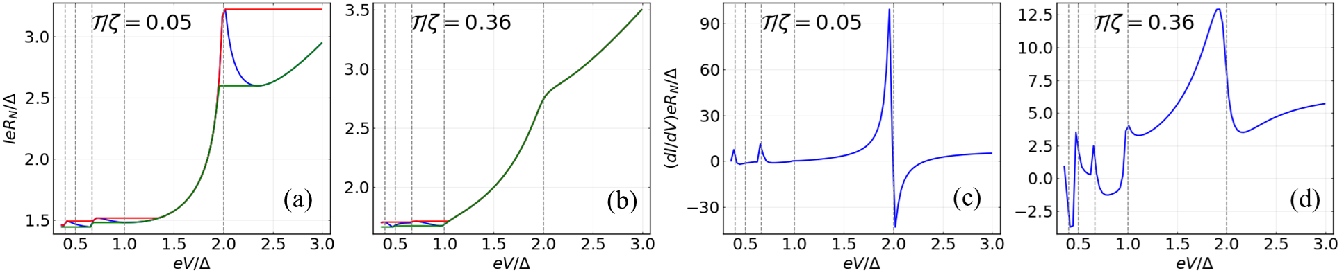
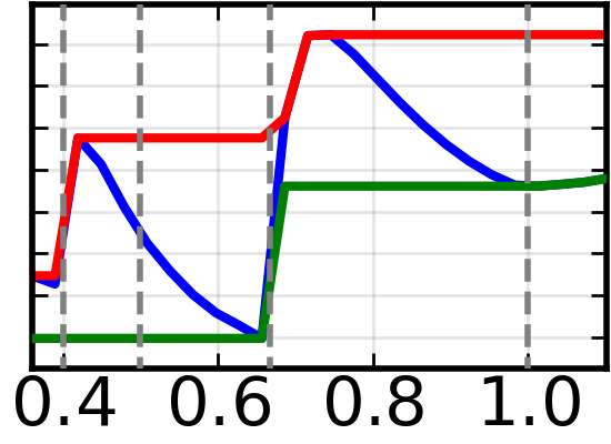
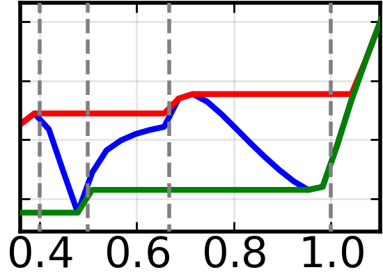
Figure 1: Exact IVCs using our non-perturbative numerical method in Eq. (3) and the corresponding differential conductance for a DC current bias with varying $\mathcal{T}$. In (a-b), the upper (red) and lower (green) envelopes of the current show the theoretically predicted hysteresis loops (inset: zoomed view of sub-gap region). The even subharmonics $e\langle V\rangle=2\Delta/n$, which are absent for $\mathcal{T}/\zeta=0.05$, appear with increasing $\mathcal{T}$. Simultaneously, all subharmonic peaks are increasingly smoothened. Gray dashed lines mark the subharmonics $2\Delta/n$. The transparency is given by $4(\mathcal{T}/\zeta)^{2}/[1+(\mathcal{T}/\zeta)^{2}]^{2}$. We use $\Gamma=0.01\Delta$, and $\zeta=5\Delta$.

This periodicity makes the problem suitable for the Floquet formalism [48, 49, 50, 51, 52, 53]. Only the tunneling Hamiltonian has a non-trivial Floquet transform in the Floquet Nambu Keldysh space,

$$\frac{1}{T}\int_{0}^{T}H_{\mathcal{T}}(\tau)e^{i\Omega\tau}d\tau=-\mathcal{T}\left(\begin{array}[]{cc}0&W_{m}\\ W_{-m}^{*}&0\end{array}\right),$$ (2)

where $\Omega=e\langle V\rangle$ is the fundamental Floquet frequency and $W_{m}=\int_{0}^{T}e^{-i\phi(\tau)/2}e^{i\Omega\tau}d\tau/T$. Since $H_{\mathcal{T}}(t+T_{0})=-H_{\mathcal{T}}$, only odd harmonics $W_{(2n-1)}$ $\forall n\in\mathbb{Z}$ are admitted in its Floquet formalism [13]. This implies that electrons(holes) gain(lose) energy in odd multiples of $e\langle V\rangle$ upon tunneling, with the amplitude $W_{m}(W_{-m}^{*})$.

We obtain the Floquet components $I_{k\Omega}$ of the current $I(t)$ across superconductors [54, 40, 50, 53] as

$$\begin{split}I_{k\Omega}=&\sum_{m,n}e\textstyle\int\limits_{0}^{\Omega}d\omega\ \mathbf{Tr}\bigg{[}\begin{matrix}\tau_{3}\Sigma_{T,LR,(n+k)m}G_{RL,mn}^{<}(\omega)\\ -(L\leftrightarrow R)\end{matrix}\bigg{]}\end{split}$$ (3)

with the lesser Green’s function $G^{<}=G^{r}\Sigma^{<}G^{a}$ [60, 64, 66, 65, 67], where $G^{r/a}$ are the full retarded/advanced Green’s function dressed by tunneling, with all matrices being in the combined Floquet Nambu Keldysh space. We note that a DC current bias $I_{\text{DC}}$ can yield multi-valued DC voltage responses, resulting in the hysteresis of IVC [Fig. 1(a-b)]. On the contrary, for any DC voltage $\langle V\rangle$ and its Floquet frequency $\Omega$, unique $W_{m}$’s are determined. Hence, we solve for $W_{m}$’s, equally $\phi(t)$, satisfying $I_{k\Omega}|_{k\neq 0}=0$ in Eq. (3) for a given $\Omega$, and find the DC current bias as $I_{0}$. The numerical solution, inspired by Ref. [13], is described in Appendix A. Crucially, we obtain the non-perturbative Green’s functions using matrix inversions instead of perturbative summation, thereby circumventing the divergence present in the latter [37, 55].

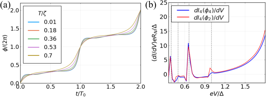
Figure 2: (a) Numerically obtained nonperturbative superconducting phase $\phi(t)$ at DC current bias. $\phi(t)$ exhibits steps at $\phi\approx\pi/2+2\pi,\pi/2+4\pi,\cdots$, separated by $T_{0}$. (b) Differential conductance at $\mathcal{O}(\mathcal{T}^{4})$. Even subharmonics appear in both $dI_{4}[\phi_{2}]/dV$ and $dI_{4}[\phi_{4}]/dV$. Gray lines mark the subharmonics $2\Delta/n$. We use $\mathcal{T}=0.12\zeta$, $\Gamma=0.005\Delta$, and $\zeta=5\Delta$.

Numerical results.—The non-perturbative numerical calculation for arbitrary transparencies presents both odd and even integer factions of SGS in IVC (Fig. 1). Our calculation shows that the missing even subharmonics emerge with increasing transparency of the junction [11, 16]. At the same time, all subharmonic peaks get commensurately smeared as the gap-edge singularity in the superconducting density of states is renormalised by tunneling.

We provide the non-perturbative numerical calculation of the superconducting phase $\phi(t)$ in Fig. 2(a), which facilitates a perturbative scheme investigating the origin of even subharmonics. To illustrate this, we consider two approximated solutions $\phi_{2}(t)$ and $\phi_{4}(t)$, each obtained from Eq. (3) but expanded upto $\mathcal{O}(\mathcal{T}^{2})$ and $\mathcal{O}(\mathcal{T}^{4})$. We expand the DC component of Eq. (3) upto $\mathcal{O}(\mathcal{T}^{2\alpha})$ with $I_{2\alpha}=\sum_{\nu=1}^{\alpha}I^{(2\nu)}$, where $I_{\infty}$ is the non-perturbative resummation of Eq. (3) and $I^{(2\nu)}\sim(\mathcal{T}/\zeta)^{(2\nu)}$ [57, 55, 58] (see Appendix B). Then, $I_{4}[\phi_{4}]=I^{(2)}[\phi_{4}]+I^{(4)}[\phi_{4}]$ already generates all integer fractions in SGS. Remarkably, we obtain all subharmonics even by plugging $\phi_{2}$ into $I_{4}[\phi_{2}]$ instead $\phi_{4}$ [Fig. 2(b)], while $I_{2}[\phi_{2}]$ does not yield even subharmonics. Therefore, the even integer fractions in SGS emerge from microscopic tunnel processes captured by the $\mathcal{O}(\mathcal{T}^{4})$ current, but overlooked in the $\mathcal{O}(\mathcal{T}^{2})$ Werthamer theory.

Microscopic origin of SGS.—We explain the microscopic origin of SGS by two complementary pictures. The time-domain picture illustrates that SGS occurs due to self-coupling of retarded responses with associated resonance condition. The frequency-domain picture explains the SGS via energy transfer in microscopic tunneling processes. Both pictures reveal that the even number of quasiparticle tunneling is essential for the even integer fractions in SGS.

Let us begin with the time-domain picture and derive the particular voltages exhibiting SGS. Since a DC current bias generates a train of sharp voltage pulses if $\langle V\rangle\leq 2\Delta/e$ [Fig. 2(a)], we adopt an ansatz $\phi(t)$ exhibiting multiple steps increased by $2\pi$ and spaced with $T_{0}=\pi/(e\langle V\rangle)$ in time. Then, we calculate the DC component $I$ of the supercurrent $I_{s}(t)$ for IVC. We analyze the pair current $I_{s}(t)=\sum_{\nu=1}^{\infty}I_{s}^{(2\nu)}(t)$ perturbatively in tunnel strength $\mathcal{T}^{2\nu}$, allowing $2\nu e$-charge tunneling. To facilitate the perturbative analysis of $I_{s}(t)$, we define $\mathcal{I}^{(2\nu)}_{s}(t)$ so that

$$I^{(2\nu)}_{s}(t)=\Im\{e^{-2i\nu\phi(t)}\mathcal{I}^{(2\nu)}_{s}(t)\}$$ (4)

Without loss of generality, we restrict here to the pair current. Our key results remain unchanged for the quasiparticle currents.

First, we study the $\mathcal{O}(\mathcal{T}^{2})$-tunneling [16] by analyzing,

$$\mathcal{I}^{(2)}_{s}(t) =\int_{-\infty}^{t}e^{i[\phi(t)-\phi(t^{\prime})]/2}\mathcal{K}_{s}(t-t^{\prime})dt^{\prime},$$ (5)

where $\mathcal{K}_{s}(\tau)$ captures the electronic retardation and oscillates at frequency $2\Delta$, stemming from the singular density of states at the superconducting gap-edges [72, 16, 54] (see Supplemental Material for details [75]). Using integration by parts, we separate $\mathcal{I}^{(2)}_{s}(t)=I_{c}^{(2)}+\delta\mathcal{I}^{(2)}_{s}(t)$ into equilibrium Cooper pair tunneling and nonequilibrium quasiparticle tunneling from slow- and fast-varying components of $\phi(t)$ with (see Appendix C)

$$\delta\mathcal{I}^{(2)}_{s}(t)=ie\int_{-\infty}^{t}\,V(t^{\prime})e^{i[\phi(t)-\phi(t^{\prime})]/2}\mathcal{J}^{(2)}_{1}(t-t^{\prime})dt^{\prime},$$ (6)

where $\mathcal{J}^{(2)}_{1}(\tau)=\int_{\tau}^{\infty}d\tau^{\prime}\mathcal{K}_{s}(\tau)$ and $I_{c}^{(2)}=\pi\Delta/(2eR_{N})$ is the critical current [75]. For a small voltage $eV(t)\ll\Delta$, $\delta\mathcal{I}^{(2)}_{s}$ is negligible, recovering the DC Josephson current $I_{s}^{(2)}(t)=I_{c}^{(2)}\sin[\phi(t)]$. Especially, focusing on a slow-varying $\phi(t)$ but exhibiting a sharp voltage pulse at $t=t_{0}$ with $2\pi$-phase jump, we find

$$\mathcal{I}^{(2)}_{s}(t)=I_{c}^{(2)}-2e^{i[\phi(t)-\phi(t^{+}_{0})]/2}\mathcal{J}^{(2)}_{1}(t-t_{0}),$$ (7)

where $t^{+}_{0}\equiv t_{0}+0^{+}$ (see Appendix C). The nonequilibrium quasiparticle excitation generated by the voltage pulse is relaxed according to energy-time uncertainty. Then, the retarded current response occurs with $\mathcal{J}_{1}^{(2)}$. The fractional phase shift $e^{i[\phi(t)-\phi(t^{+}_{0})]/2}$ in Eq. (7) stems from the dynamical phase of the nonequilibrium tunneling state with an excessive $1e$-charge with respect to the BCS ground state.

We study IVC with the DC component of the supercurrent $I_{s}^{(2)}(t)$ applying a superposition principle (SP) of nonequilibrium quasiparticle tunneling. By decomposing $V(t)=\sum_{p=0}^{\infty}V_{p}(t)$ into well-separated voltage pulses $V_{p}(t)$ at $t_{p}=-pT_{0}$, we find the SP

$$\delta\mathcal{I}^{(2)}_{s}[V]=\sum_{p=0}^{\infty}e^{ie\int_{t_{p}^{+}}^{t}dt^{\prime}V(t^{\prime})}\delta\mathcal{I}^{(2)}_{s}[V_{p}],$$ (8)

which is a quasilinear functional of $V(t)$ with fractional phase shifts [75].

Applying the SP in Eq. (8) to a train of voltage pulses with the ansatz $\phi(t)$ of multiple steps increased by $2\pi$ at $t=0,-T_{0},\cdots$, we find

$$I_{s}^{(2)}(t)=I_{c}^{(2)}\sin[\phi(t)]-2\sum_{p=0}^{\infty}(-1)^{p}\mathcal{J}^{(2)}_{1}(t+pT_{0}).$$ (9)

The DC component of the first term yields RSJ-like IVC. The second term leads to SGSs at particular voltages, as the retarded responses $(-1)^{p}\mathcal{J}^{(2)}_{1}(t+pT_{0})$ constructively interfere adding to DC components of $I_{s}^{(2)}(t)$. Deriving the asymptotic expression of $\mathcal{J}^{(2)}_{1}(t)\sim e\Delta\mathcal{T}^{2}\sin(2t\Delta)\Theta(t)/(t\Delta\zeta^{2})$ for $1<t\Delta$, we find the resonance condition of the self-coupling as $2T_{0}\Delta+\pi=2n\pi$ and SGSs at $e\langle V\rangle=2\Delta/(2n-1)$, yielding a similar IVC to Fig. 1(c). We highlight that sign flips $(-1)^{p}$ in Eq. (9) stem from excessive $1e$-excitation. They are responsible for the missing even integer fractions in SGS.

We show that the even integer fractions $2\Delta/(2ne)$ in SGS stem from the self-coupling of quasiparticle tunneling with excessive $2e$-excitations appearing at $\mathcal{O}(\mathcal{T}^{4})$. Starting with the pair current, we obtain three distinct contributions $\mathcal{I}_{s}^{(4)}(t)=\sum_{j=1}^{3}\mathcal{I}_{s,j}^{(4)}(t)$. Since the essential properties relevant to our discussion remain unchanged. Between the contribution, we focus only on $I_{s,1}^{(4)}(t)$ here. As before, we separate $\mathcal{I}^{(4)}_{s,j}(t)=I^{(4)}_{c,j}+\delta\mathcal{I}^{(4)}_{s,j}(t)$ [75]. Assuming the same step ansatz $\phi(t)$ as for Eq. (9), we derive

$$\delta\mathcal{I}^{(4)}_{s,1}(t)=\sum_{k=1}^{3}\sum_{p=0}^{\infty}e^{ik[\phi(t)-\phi(-pT_{0}^{+})]/2}\mathcal{J}_{k}^{(4)}(t+pT_{0}),$$ (10)

where $\mathcal{J}_{1,2,3}^{(4)}(t)$ corresponds to the nonequilibrium tunneling accompanied by the excessive excitations of $1e$, $2e$, $3e$, which oscillate with the frequency $2\Delta$ and decay in time as $\mathcal{J}_{1}^{(2)}(t)$. The retarded response accompanied by $2e$-excitation $\mathcal{J}_{2}^{(4)}(t)$ plays an essential role for even integer fractions in SGS, whose asymptotic expression is $\mathcal{J}^{(4)}_{2}(t)\sim e\Delta\mathcal{T}^{4}\cos(2t\Delta-3\pi/4)\Theta(t)/(\sqrt{t\Delta}\zeta^{4})$ for large argument $1<t\Delta$, yielding the resonant self-coupling condition, $2T_{0}\Delta=2n\pi$. Consequently, $2e$-excitations at $\mathcal{O}(\mathcal{T}^{4})$-tunneling give rise to the even integer fraction of SGS, $e\langle V\rangle=2\Delta/(2n)$.

Comprising the $\mathcal{O}(\mathcal{T}^{2})$- and $\mathcal{O}(\mathcal{T}^{4})$-tunneling constitutes similar SGS to Fig. 2(b). We find that the tunneling process at $\mathcal{O}(\mathcal{T}^{2\nu})$ with $2\nu e$-charge allows only equilibrium pair current, while nonequilibrium quasiparticle currents are mediated with $1e,\cdots,(2\nu-1)e$-excitations [75]. Hence, $\mathcal{O}(\mathcal{T}^{2})$-tunneling is a particular case allowing only the odd number of charge excitation, resulting in the missing even series in SGS.

Next, we present the frequency-domain picture to better illustrate the microscopic tunneling processes accompanied by excessive quasiparticle excitations. The current and the underlying electronic tunnel pathways, are independent of the biasing scheme (current vs. voltage bias). Hence, the conditions for subharmonics, expressed in terms of $W_{m}$, are universal irrespective of biasing scheme and specific to the order in $\mathcal{T}/\zeta$ at which the current is evaluated. Note that $W_{m}$ represents the dynamical phase acquired by electrons upon tunelling across the biased barrier region. Consequently, $W(\omega)$ is the amplitude for the excitation of tunneling quasiparticles by energy $\omega$ [68, 54]. Subharmonics arise only when this excitation energy satisfies the universal conditions specified below. As described in Appendix B, the perturbative contributions to the DC current are given by

$$\frac{I_{\text{DC}}^{(2)}}{\mathcal{T}^{2}}= \textstyle\int\limits_{-\infty}^{\infty}\hskip-3.99994pt\frac{d\omega}{2\pi}\prod\limits_{j=1}^{2}\frac{d\omega_{j}}{2\pi}\delta\big{(}\sum_{l=1}^{2}\omega_{j}\big{)}\mathbf{tr}\big{[}\tau_{3}\Sigma^{T}_{LR}(\omega_{1})$$

$$\big{(}g(\omega+\omega_{2})\Sigma^{T}_{RL}(\omega_{2})g(\omega)\big{)}^{<}-(L\leftrightarrow R)\big{]},$$ (11a)

$$\frac{I_{\text{DC}}^{(4)}}{\mathcal{T}^{4}}= \textstyle\int\limits_{-\infty}^{\infty}\hskip-3.99994pt\frac{d\omega}{2\pi}\prod\limits_{j=1}^{4}\frac{d\omega_{j}}{2\pi}\delta\big{(}\sum_{l=1}^{4}\omega_{j}\big{)}\mathbf{tr}\big{[}\tau_{3}\Sigma^{T}_{LR}(\omega_{1})$$ (11b)

$$\big{(}g(\omega+\omega_{2}+\omega_{3}+\omega_{4})\Sigma^{T}_{RL}(\omega_{2})g(\omega+\omega_{3}+\omega_{4})$$

$$\Sigma^{T}_{LR}(\omega_{3})g(\omega+\omega_{4})\Sigma^{T}_{RL}(\omega_{4})g(\omega)\big{)}^{<}-(L\leftrightarrow R)\big{]},$$

where each instance of the tunneling self-energy $\Sigma^{T}(\omega)$, depending on $W(\omega)$ (see Appendix A), corresponds to a single tunnel event. Similar expressions can be obtained for higher orders. From Eq. (11), we find two types of terms: (i) usual MAR-like processes where all tunnel events exchange the same magnitude of energy, and (ii) processes where different tunnel events exchange different energies. Note that type (ii) is not allowed in $I_{\text{DC}}^{(2)}$. We emphasise that for a DC voltage bias $V_{\text{DC}}$, since $W(t)=e^{-ieV_{\text{DC}}t}$ is monochromatic, only type (i) contributes with the exchanged energy equalling $\Omega=eV_{\text{DC}}$. However, for a DC current bias, an AC voltage with mean value $\langle V\rangle$ develops, with $W(\omega)$ containing all odd multiples of $\Omega=e\langle V\rangle$ [explained below Eq. (3)]. Hence, both processes (i) and (ii) contribute to IVC for a DC current bias, with the energy exchanged including all these values.

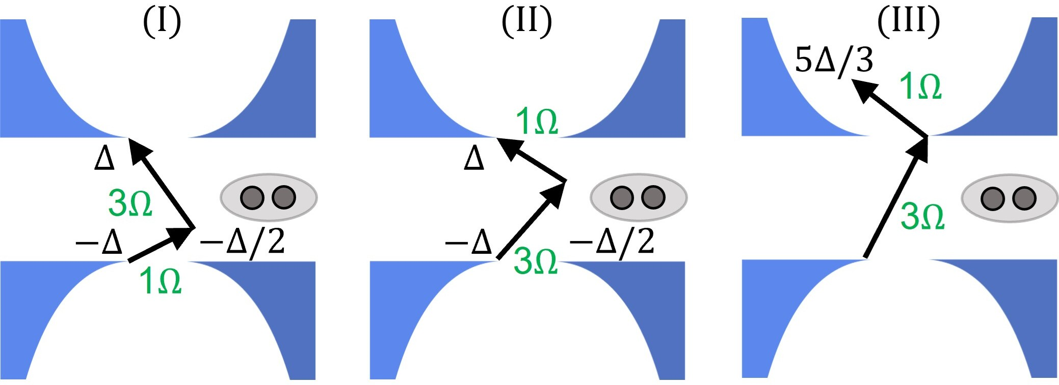
Figure 3: (I-III) Illustration of resonant type-(ii) processes in $I_{\text{DC}}^{(4)}$, for $a=1$ and $b=3$ without loss of generality, all of them transferring 2 electrons/1 pair. The density of states is shown in blue, and arrows depict tunneling quasiparticles. The corresponding currents are detailed in Appendix D.

Starting with a DC Werthamer current $I_{\text{DC}}^{(2)}$ at $\mathcal{O}(\mathcal{T}^{2})$ [11], resonant transport is only possible at $\Omega=2\Delta$ by exciting a single quasiparticle from the lower band-edge of one lead to the upper band-edge of the other lead. This defines the universal singularity condition. Indeed for a DC voltage bias, with $W(\omega)=2\pi\delta(\omega-eV_{\text{DC}})$, $I_{\text{DC}}^{(2)}$ exhibits only the Riedel peak at $eV_{\text{DC}}=2\Delta$, and no subharmonics [69, 11]. For a DC current bias at $\mathcal{O}(\mathcal{T}^{2})$, we have only type (i) processes exchanging energies $(2n-1)\Omega$ $\forall n\in\mathbb{Z}^{+}$ with $\Omega=e\langle V\rangle$, which follows from the spectral decomposition of $W(\omega)$. Therefore, we obtain only the odd subharmonic singularities at $(2n-1)\Omega=(2n-1)e\langle V\rangle=2\Delta$.

Process	DC V bias	DC I bias
	$\Omega=eV_{\mathrm{DC}}$ $a,b=1$	$\Omega=e\langle V\rangle$ $a,b=\text{odd}$
(a,b):$(a\pm b)\Omega=2\Delta$	$eV_{\mathrm{DC}}=\frac{2\Delta}{2}$	$e\langle V\rangle=\frac{2\Delta}{2n}$
(c):$(a,b)\Omega=2\Delta$	$eV_{\mathrm{DC}}=2\Delta$	$e\langle V\rangle=\frac{2\Delta}{2n-1}$

Table 1: Conditions for singularities for both DC voltage and DC current biases, for the type (ii) processes in Fig. 3.

This argument extends to the $\mathcal{O}(\mathcal{T}^{4})$ DC current $I_{\text{DC}}^{(4)}$. For a DC voltage bias with only type (i) processes, an additional singularity occurs at $eV_{\text{DC}}=2\Delta/2$ (Appendix E), which is the first-order DC MAR current [37, 70, 71]. This resonance is a two-step excitation (one Andreev reflection), with each step exciting the quasiparticle by $eV_{\text{DC}}=2\Delta/2$. Thus, the $\mathcal{O}(\mathcal{T}^{4})$ singularity condition for type (i) processes is $\Omega=2\Delta/2$ and $2\Delta$. For a DC current bias providing all odd multiples of $\Omega=e\langle V\rangle$, we obtain additional singularities at $(2n-1)\Omega=(2n-1)e\langle V\rangle=2\Delta/2$, generating all even subharmonics except for $e\langle V\rangle=2\Delta/(4n)$. Pursuing this to higher orders (Appendix E), we find that for type (i) processes with a DC voltage bias, the singularity at $\Omega=eV_{\text{DC}}=2\Delta/n$ appears first in $I_{\text{DC}}^{2n}\sim\mathcal{T}^{2n}$ [37]. Hence, considering only type (i) process, the subharmonic at $e\langle V\rangle=2\Delta/4n$ appears first in $I_{\text{DC}}^{(8n)}$ even for a DC current bias. Remarkably, considering also type (ii) processes, we find that all subharmonics may be obtained already in $I_{\text{DC}}^{(4)}$. As illustrated in Fig. 3, combining two energy exchanges $\Omega_{1}=a\Omega$ and $\Omega_{2}=b\Omega$ yields singularities at $(a+b)\Omega=2\Delta$, $(a-b)\Omega=2\Delta$, $a\Omega=2\Delta$, and $b\Omega=2\Delta$, constituting the $\mathcal{O}(\mathcal{T}^{4})$ universal singularity condition (Appendix E). The resonant energy exchanges $\Omega_{1,2}$ ensure that the tunnel pathways exploit at the gap edges either the enhanced quasiparticle density of states for tunneling, or the enhanced pairing tendency. Consequently, for a DC current bias, the subharmonics at $\Omega=e\langle V\rangle=2\Delta/(4n)$ may be obtained from any suitable combination $\Omega_{1}=ae\langle V\rangle$ and $\Omega_{2}=(4-a)e\langle V\rangle$. A similar analysis applies to the pure pair current (Appendix F). Hence, unlike a DC voltage bias, the wide spectrum of energies supplied by the time-varying voltage for a DC current bias exhausts all possible resonant tunnel pathways. Our treatment provides a unified approach for both, as summarised in Table 1. Finally, note that the higher harmonics in $W(\omega)$ are increasingly attenuated. Furthermore, higher order currents $I_{\text{DC}}^{(2n)}$ are suppressed by the transparency $(\mathcal{T}/\zeta)^{(2n)}$. Consequently higher current subharmonics are progressively suppressed with increasing subharmonic order.

Conclusion.—We provide a microscopic theoretical solution for DC current-biased Josephson junctions with arbitrary junction transparencies. Transcending the Werthamer theory, which is the leading second-order term in tunnel coupling and fails to match experiments, we find that the next, fourth-order term generates the missing even subharmonics for high transparencies. We propose that the necessary condition for this observation is the tunneling of an even number of intermediate quasiparticles.

Given the recent discoveries a variety of superconductors and the increasing quality of junctions, our microscopic theory is highly relevant for interpreting present-day experiments, reaching new type of Josephson effects beyond conventional phenomenological approaches. The advancements in experimental techniques and materials underscore the pressing need for a microscopic framework to bridge the gap between theory and experiment.

I End Matter

Appendix A.—Here, we describe the numerical techniques to solve the current-biased problem, leading to Fig. 2(a).

Within this formalism, the Keldysh Green’s functions are expanded as,

$$G(t,t^{\prime})=\sum_{m,n}\int_{0}^{\Omega}\frac{d\omega}{2\pi}e^{-i(\omega+m\Omega)t}e^{i(\omega+n\Omega)t^{\prime}}G_{mn}(\omega),$$ (12)

where the fundamental Floquet frequency $\Omega=2\pi/T=e\langle V\rangle$, and the functions $G_{mn}(\omega)\coloneqq G_{m-n}(\omega+\Omega(m+n)/2)$ satisfy $G_{mn}(\omega+k\Omega)=G_{(m+k)(n+k)}(\omega)$. The (Keldysh) Dyson equation becomes $G_{mn}(\omega)=g_{mn}(\omega)+\sum_{k}g_{mk}(\omega)\Sigma_{kk^{\prime}}(\omega)G_{k^{\prime}n}(\omega)$, where the Green’s functions are matrices in Floquet Keldysh Nambu space, and $g_{mn}(\omega)=g(\omega+m\Omega)\delta_{mn}$ is defined in the absence of $H_{\mathcal{T}}$.

The self-energy contains three terms: (i) $\Sigma_{\mathcal{T}}$ arising from $H_{\mathcal{T}}$, given by $\Sigma^{r/a}_{T,LR,,m-n}={\Sigma^{r/a}}^{*}_{T,RL,n-m}=\int_{0}^{T}H_{\mathcal{T}}(\tau)e^{i(m-n)\Omega\tau}d\tau/T=-\mathcal{T}[W_{m-n}\tau_{+}+W_{-(m-n)}^{*}\tau_{-}]$, where $W_{a}$ is the Floquet transform of $W(t)=e^{-i\phi(t)/2}$, and $\tau_{\pm}=(\tau_{0}\pm\tau_{3})/2$ with $\tau_{\mu}$ denoting the Pauli matrices in Nambu space. The lesser component vanishes [40]. (ii) $\Sigma^{r/a}_{\Gamma}=\pm i\Gamma/2$ and $\Sigma^{<}_{\Gamma}=-i\Gamma f(\omega)$, where $f(\omega)$ is the Fermi function. Apart from aiding numerical convergence, it accounts for the broadening/lifetime arising from, e.g., relaxation to the high-energy quasiparticle continuum, electron-phonon interactions, etc [54]. (iii) $\Sigma_{\zeta}$, resulting from coupling the central device region composed of single-site leads  [59] to semi-infinite superconducting reservoirs [60]. Specifically, $\Sigma^{r/a/<}_{\zeta}=(-\zeta/2)^{2}\tau_{3}g^{r/a/<}\tau_{3}$ where $g^{r/a/<}$ is the boundary Green’s function [61, 62, 60, 40, 63].

Following Ref. [13], we consider (truncate) $4N_{F}+1$ Floquet modes $W_{n}$ for the factor $W(t)=e^{-i\phi(t)/2}$, ranging from $-2N_{F}\Omega$ through $2N_{F}\Omega$. $W(t)$ satisfies $W(t+T_{0})=-W(t)$, and thus only the odd harmonics $W_{(2n-1)}$ are non-zero. This corresponds to $4N_{F}$ unknown variables since $W$ is complex. The Floquet modes of the Green’s functions and the current lie in the range $-N_{F}\Omega$ to $N_{F}\Omega$. The first $2N_{F}$ equations to be solved are obtained by setting the even Floquet modes of the current to zero. The odd modes vanish naturally for conventional superconductors. We obtain $2N_{F}-1$ additional equations from the condition $W(t)W(t)^{*}=1$. The final equation is $\phi(t=0)=0$. These are solved for different values of $\Omega=e\langle V\rangle$. This amounts to obtaining the AC voltage $(1/2e)(d\phi/dt)$ with the mean value $\langle V\rangle$ which generates a DC current. The quasiparticles repeatedly tunnel (Andreev process) until they escape into the continuum. Thus, the required $N_{F}$ for a convergent solution scales as $2\Delta/eV$. In all of our numerical plots, we choose a sufficiently large value of $N_{F}$ to ensure convergence. In practice, for the range of parameters employed in our work, we find $N_{F}\gtrsim 20$ works well. Specifically, in Fig. 1, we use $N_{F}=34$.

Here we show that our exact expression for the current reduces to the Werthamer current [11]. To this end, we expand $G^{<}=g^{<}+\delta{G^{<}}^{(1)}$ with $g^{<}=g^{r}\Sigma^{<}g^{a}\sim\mathcal{O}(1)$, and $\delta{G^{<}}^{(1)}=(g^{r}\Sigma_{T}g^{<}+g^{<}\Sigma_{T}g^{a})$ being the leading $\mathcal{O}(\mathcal{T})$ correction due to tunneling. Note that $g^{r/a/<}$ include the broadening $\Gamma$ with $g^{<}=g^{r}\Sigma^{<}_{\Gamma}g^{a}$, but not tunneling (see [67]). The corresponding $\mathcal{O}(\mathcal{T}^{2})$ current $I(t)=e\Re\ \mathbf{Tr}\int_{-\infty}^{\infty}dt^{\prime}\tau_{3}H_{T}(t)\big{(}g^{r}(t-t^{\prime})H_{T}(t^{\prime})g^{<}(t^{\prime}-t)+g^{<}(t-t^{\prime})H_{T}(t^{\prime})g^{a}(t^{\prime}-t)\big{)}$ is the Werthamer current [11, 54].

Appendix B.—Using the Langreth rules [56], the $\sim\mathcal{T}^{\nu}$ contribution to the lesser Green’s function is given by,

$$\delta{G^{<}}^{(\nu)}=\sum_{i=1}^{\nu}\bigg{(}\prod_{j=1}^{i-1}g_{j}^{r}\Sigma^{r}_{j}\bigg{)}g_{i}^{<}\bigg{(}\prod_{k=i+1}^{\nu}\Sigma^{a}_{k}g_{k}^{a}\bigg{)}.$$ (13)

Hence, from Eq. (3), for any given $\alpha>0$ the $\mathcal{O}(\mathcal{T}^{2\alpha})$ current admits the expansion

$$I_{2\alpha}=\sum_{\nu=1}^{\alpha}\underbrace{\bigg{(}\sum_{m,n}e\mathbf{Tr}\bigg{[}\begin{matrix}\tau_{3}\Sigma_{T,LR,(n+k)m}\delta G_{RL,mn}^{<,(2\nu-1)}\\ -(L\leftrightarrow R)\end{matrix}\bigg{]}\bigg{)}}_{I^{(2\nu)}},$$ (14)

containing a sum of contributions $I^{(2\nu)}\sim\mathcal{T}^{2\nu}$ upto $\nu=\alpha$.

Appendix C.—We provide the detailed derivation yielding $\mathcal{I}^{(2)}_{s}(t)=I^{(2)}_{c}+\delta\mathcal{I}^{(2)}_{s}(t)$ in the main text. Applying integration by part to Eq. (5), we obtain

$$\mathcal{I}^{(2)}_{s}(t) =e^{\frac{i}{2}\phi(t)}\left\{\left[e^{-\frac{i}{2}\phi(t^{\prime})}\mathcal{J}^{(2)}_{1}(t-t^{\prime})\right]\Big{|}_{t^{\prime}=-\infty}^{t^{\prime}=t}\right.$$ (15)

$$\left.+ie\int_{-\infty}^{t}V(t^{\prime})e^{-\frac{i}{2}\phi(t^{\prime})}\mathcal{J}^{(2)}_{1}(t-t^{\prime})dt^{\prime}\right\},$$

where $\mathcal{J}^{(2)}_{1}(t-t^{\prime})$ is a primitive function of $\mathcal{K}_{s}(t-t^{\prime})$ (see Ref. [75] for the definition). To decompose $\mathcal{I}^{(2)}_{s}(t)$ into two contributions from slow- and fast-varying $\phi(t)$, we consider a small voltage $eV(t)\ll\Delta$ first and find a suitable choice of the boundary condition of $\mathcal{J}^{(2)}_{1}$ yielding $I^{(2)}_{s}(t)\propto\sin[\phi(t)]$. The boundary condition is $\mathcal{J}^{(2)}_{1}(\infty)=0$ and $\mathcal{J}^{(2)}_{1}(0)=I_{c}^{(2)}$, which hold if $\mathcal{J}^{(2)}_{1}(t-t^{\prime})\equiv\int_{t-t^{\prime}}^{\infty}\mathcal{K}_{s}(\tau)d\tau$. Consequently, we separate $\mathcal{I}^{(2)}_{s}(t)=I_{c}^{(2)}+\delta\mathcal{I}^{(2)}_{s}(t)$. Indeed, $\mathcal{J}^{(2)}_{1}(0)=\pi\Delta/(2eR_{N})$, yielding the critical current at $\mathcal{O}(\mathcal{T}^{2})$.

We provide a detailed derivation of Eq. (7) in the main text. We consider an abrupt phase jump at $t=t_{0}$ with a slow-varying phase $\phi_{0}(t)$ as

$$\phi(t)=\left\{\begin{array}[]{ll}\phi_{0}(t),&\quad t<t_{0},\\ \phi_{0}(t)+\frac{\delta\phi}{\delta t}(t-t_{0}),&\quad t_{0}<t<t_{0}+\delta t,\\ \phi_{0}(t)+\delta\phi,&\quad t_{0}+\delta t<t,\end{array}\right.$$ (16)

where $\phi_{0}^{\prime}(t)\ll 2e\Delta$. Then, the nonzero value of Eq. (6) is obtained only for $t>t_{0}+\delta t$ as follows.

$$\delta\mathcal{I}^{(2)}_{s}(t)$$ (17)

$$\,=\frac{ie^{\frac{i\phi(t)}{2}}\delta\phi}{2\delta t}\int_{t_{0}}^{t_{0}+\delta t}e^{-\frac{i\delta\phi(t^{\prime}-t_{0})}{2\delta t}}e^{-\frac{i\phi_{0}(t^{\prime})}{2}}\mathcal{J}^{(2)}_{1}(t-t^{\prime})dt^{\prime}$$

$$\,=-e^{\frac{i\phi(t)}{2}}(e^{-\frac{i\phi(t_{0}+\delta t)}{2}}-e^{-\frac{i\phi(t_{0})}{2}})\mathcal{J}^{(2)}_{1}(t-t_{0})+\mathcal{O}(\delta t),$$

where $e^{-i\phi_{0}(t^{\prime})/2}\mathcal{J}^{(2)}_{1}(t-t^{\prime})$ is expanded upto $\mathcal{O}(\delta T)$. Taking $\delta t\rightarrow 0$ and $\delta\phi=2\pi$, this yields Eq. (7). In the main text, the Heaviside function $\Theta(t-t_{0})$ is absorbed into the asymptotic expression of $\mathcal{J}^{(2)}_{1}(t-t_{0})$.

Appendix D.—Here we show the three kinds of resonant terms in Eq. (11), corresponding to Fig. 3.

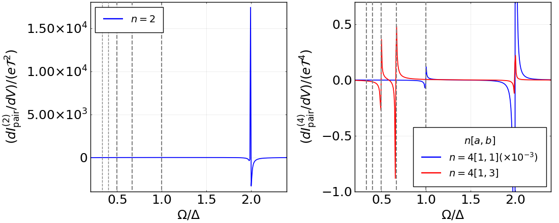
Figure 4: The normalised differential conductance $(dI_{\text{DC}}^{(n)}/dV)/\mathcal{T}^{n}$ for (left) $\mathcal{T}^{2}$ and (right) $\mathcal{T}^{4}$ for $\Omega_{1}=\Omega$ and $\Omega_{2}=3\Omega$ pair currents. We find the same universal singularity conditions as in Fig. 5.

$$(a) \ e\mathcal{T}^{4}\big{[}W_{-1}g_{12,R}(-\tfrac{\Delta}{2})W_{-3}{\color[rgb]{1,0,0}g_{22,L}(\Delta)}{\color[rgb]{0,1,0}W_{+3}}g_{21,R}(-\tfrac{\Delta}{2}){\color[rgb]{0,1,0}W_{+1}}$$

$$\hskip 17.07164pt{\color[rgb]{1,0,0}g_{11,L}(-\Delta)}\big{]}$$ (18a)

$$(b) \ e\mathcal{T}^{4}\big{[}W_{-3}{\color[rgb]{1,0,0}g_{12,R}(\Delta)}{\color[rgb]{0,1,0}W_{-1}}g_{22,L}(2\Delta){\color[rgb]{0,1,0}W_{+3}}{\color[rgb]{1,0,0}g_{21,R}(-\Delta)}W_{+1}$$

$$\hskip 17.07164ptg_{11,L}(-2\Delta)\big{]}$$ (18b)

$$(c) \ e\mathcal{T}^{4}\big{[}W_{-3}{\color[rgb]{1,0,0}g_{12,R}(\Delta)}W_{-1}g_{22,L}(\tfrac{5\Delta}{3})W_{+1}{\color[rgb]{1,0,0}g_{21,R}(\Delta)}{\color[rgb]{0,1,0}W_{+3}}$$

$$\hskip 17.07164pt{\color[rgb]{1,0,0}g_{11,L}(-\Delta)}\big{]}$$ (18c)

Resonant Green’s functions (at frequency $\pm\Delta$) are shown in red, and the connecting energy exchanges in green. Resonance occurs when the net energy exchange joining the two red Green’s functions equals $2\Delta$. E.g., in (a) the sequence $W_{+3}W_{+1}$ transfers $(3+1)\Omega$, resulting in $\Omega=2\Delta/(3+1)$. (a) and (c) represent diagrams (I) and (III), respectively. (b), with its “asymmetric” arrangement of $W_{m}$’s, is an interference between the paths shown by diagrams (I) and (II), resonant at $\Omega=2\Delta/(3-1)$.

Appendix E.—We show the universal singularity conditions in currents at various orders of $\mathcal{T}$ in Fig. 5.

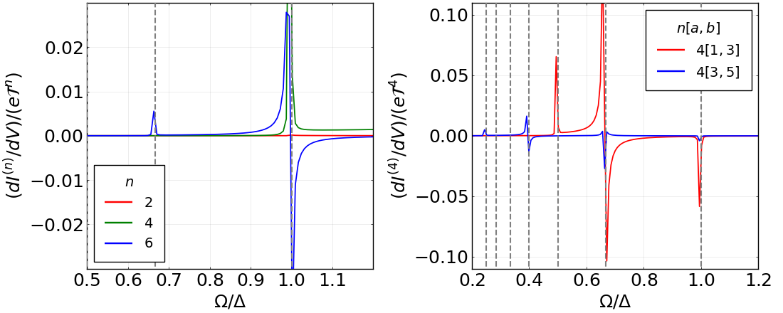
Figure 5: (a) Normalised differential conductance $(dI_{\text{DC}}^{(n)}/dV)/\mathcal{T}^{n}$ for type-(i) processes, where all tunnel events exchange the same energy $\Omega$. The singularity at $\Omega=2\Delta/n$ appears first in $I_{\text{DC}}^{(2n)}$. (b) Type-(ii) processes in $(dI_{\text{DC}}^{(4)}/dV)/\mathcal{T}^{4}$ with two different energies exchanged $\Omega_{1}=a\Omega$ and $\Omega_{2}=b\Omega$ as stated in the legend. The dashed vertical lines denote all subharmonics. The universal singularity conditions follow: $\Omega=2\Delta/a$, $2\Delta/b$, and $2\Delta/|a\pm b|$. To find the condition for the singularity in terms of the DC voltage, or mean AC voltage for a current bias, see Tab. 1.

Appendix F.—While we have shown the generalised MAR-like processes in Fig. 3 (see also Ref. [71]) which, like the usual MAR process, is a quasiparticle-mediated pair transfer, there is also a pure pair current at $\mathcal{T}^{4}$ which is the analogue of the $\mathcal{T}^{2}$ equilibrium Josephson current. They are obtained from Eq. (11) on performing the Nambu trace and retaining terms containing only the anomalous Green’s functions $g_{12}$ and $g_{21}$. Our conclusions regarding the universal singularity conditions hold for them too, as shown in Fig. 4. From Eq. (11), we obtain

$$\frac{I_{\text{DC, pair}}^{(2)}}{\mathcal{T}^{2}}= \textstyle\int\limits_{-\infty}^{\infty}\hskip-3.99994pt\frac{d\omega}{2\pi}\prod\limits_{j=1}^{2}\frac{d\omega_{j}}{2\pi}\delta\big{(}\sum_{l=1}^{2}\omega_{j}\big{)}\big{[}W(\omega_{1})$$

$$\big{(}g_{12}(\omega+\omega_{2})W(\omega_{2})g_{21}(\omega)\big{)}^{<}-\text{h.c.}\big{]},$$ (19a)

$$\frac{I_{\text{DC, pair}}^{(4)}}{\mathcal{T}^{4}}= \textstyle\int\limits_{-\infty}^{\infty}\hskip-3.99994pt\frac{d\omega}{2\pi}\prod\limits_{j=1}^{4}\frac{d\omega_{j}}{2\pi}\delta\big{(}\sum_{l=1}^{4}\omega_{j}\big{)}\big{[}W(\omega_{1})$$

$$\big{(}g_{12}(\omega+\omega_{2}+\omega_{3}+\omega_{4})W(\omega_{2})g_{21}(\omega+\omega_{3}+\omega_{4})$$

$$W(\omega_{3})g_{12}(\omega+\omega_{4})W(\omega_{4})g_{21}(\omega)\big{)}^{<}-\text{h.c.}\big{]},$$ (19b)

For a constant non-zero voltage bias $eV_{\text{DC}}$, for which $W(\omega)=2\pi\delta(\omega-eV_{\text{DC}})$, it can be checked from Eq. (19) that the DC pure pair term vanishes for all orders in $\mathcal{T}$, as it cannot dissipate heat. However, for a DC current bias with an AC voltage, there is generally a non-zero DC component of the pure pair current at all orders, even for finite voltages. This was already seen at $\mathcal{O}(\mathcal{T}^{2})$ in Refs. [13] and [16].

Supplemental Material for “Microscopic Theory of DC Current-Biased Josephson Junctions with Arbitrary Transparencies”

In this Supplemental Material, we present the standard mean-field Hamiltonian of superconductors used in the time-domain analysis, various anomalous bare Green’s functions, the derivation of the superposition principle of nonequilibrium quasiparticle tunneling, the detail calculations of $\delta\mathcal{I}_{s}^{(4)}(t)$, and the discussion of $\delta\mathcal{I}_{s}^{(2\nu)}(t)$. Here, we reintroduce $\hbar$ when it is necessary for clarity.

II Standard mean-field Hamiltonian of superconductors

We provide the standard mean-field Hamiltonian of $s$-wave superconductors and tunneling Hamiltonian adopted for the time-domain analysis in the main text. The Hamiltonian of the superconductors on left and right $H_{L}$ and $H_{R}$ are presented in the momentum space $k$,

$$H_{L} = \sum_{k,\sigma=\uparrow,\downarrow}\left[(E_{k}-\mu_{L})c_{k,\sigma,L}^{\dagger}c_{k,\sigma,L}+\Delta_{L}c_{k,\sigma,L}^{\dagger}c_{-k,-\sigma,L}^{\dagger}+\Delta_{L}^{*}c_{-k,-\sigma,L}c_{k,\sigma,L}\right],$$ (20)

$$H_{R} = \sum_{k,\sigma=\uparrow,\downarrow}\left[(E_{k}-\mu_{R})c_{k,\sigma,R}^{\dagger}c_{k,\sigma,R}+\Delta_{R}c_{k,\sigma,R}^{\dagger}c_{-k,-\sigma,R}^{\dagger}+\Delta_{R}^{*}c_{-k,-\sigma,R}c_{k,\sigma,R}\right],$$ (21)

where $\sigma$ is the spin index of electrons, and $-\sigma$ denotes the opposite direction of the spin. $\mu_{L}$ and $\mu_{R}$ are the chemical potential of left and right superconductors, respectively. In the main text, we focus on the symmetric junction with the same superconducting gap $\Delta_{L}=\Delta_{R}=\Delta$. The tunneling Hamiltonian is also presented in the momentum space,

$$H_{T}=\sum_{k,q,\sigma}\left[\mathcal{T}e^{-i\phi(t)/2}c_{k,\sigma,R}^{\dagger}c_{q,\sigma,L}+\mathcal{T}^{*}e^{i\phi(t)/2}c_{q,\sigma,L}^{\dagger}c_{k,\sigma,R}\right].$$ (22)

The tunneling matrix element $\mathcal{T}$ is related to the transition probability of an electron with the momentum $q$ on left to tunnel into the momentum state $k$ on right. It is valid to use W.K.B approximation and introduce the momentum-independent tunneling matrix element $\mathcal{T}$, if we focus on the voltages comparable to the superconducting gap or the junctions with a quantum point contact [74]. Since only the powers of $|\mathcal{T}|^{2}$ appear calculating the electrical current, we assume $\mathcal{T}$ is real without loss of generality.

III Various anomalous bare Green’s functions

We provide various anomalous bare Green’s functions of superconductors without the tunneling to each another. Although the bare Green’s functions have nothing to do with the tunneling strength $\mathcal{T}$, applying Langreth rule to obtain, the perturbative expansion of the mixed Keldysh Green’s function $\hat{G}^{<}_{LR}(t,t^{\prime})$ at $\mathcal{T}^{2\nu}$-order includes $2\nu$ of the bare Green’s functions. Noticing this, $\mathcal{T}^{2\nu}$ can be absorbed into the anomalous bare Green’s functions for convenience,

$$f^{r}(t) = \sum_{k}f^{r}_{k,q}(t)=-\frac{\Delta}{2\hbar}\frac{\mathcal{T}}{\zeta}\Theta(t)J_{0}\left(\frac{\Delta|t|}{\hbar}\right),$$ (23)

$$f^{a}(t) = \sum_{k}f^{a}_{k,q}(t)=-\frac{\Delta}{2\hbar}\frac{\mathcal{T}}{\zeta}\Theta(-t)J_{0}\left(\frac{\Delta|t|}{\hbar}\right),$$ (24)

$$f^{>}(t) = \sum_{k}f^{>}_{k,q}(t)=-\frac{\Delta}{4\hbar}\frac{\mathcal{T}}{\zeta}\text{sgn}(t)J_{0}\left(\frac{\Delta|t|}{\hbar}\right)+i\frac{\Delta}{4\hbar}\frac{\mathcal{T}}{\zeta}Y_{0}\left(\frac{\Delta|t|}{\hbar}\right),$$ (25)

$$f^{<}(t) = \sum_{k}f^{<}_{k,q}(t)=\frac{\Delta}{4\hbar}\frac{\mathcal{T}}{\zeta}J_{0}\left(\frac{\Delta|t|}{\hbar}\right)+i\frac{\Delta}{4\hbar}\frac{\mathcal{T}}{\zeta}Y_{0}\left(\frac{\Delta|t|}{\hbar}\right),$$ (26)

where we evaluate the real-time Green’s functions at zero temperature using the BCS approximation of the pair density of states [74],

$$p(\omega)=\frac{\Delta}{\sqrt{\omega^{2}-\Delta^{2}}}\Theta(|\omega|-\Delta).$$ (27)

Here, $J_{0}$ and $Y_{0}$ are Bessel functions of the first and second kind, respectively. The normal resistance is inversely proportional to $\mathcal{T}^{2}$ as $1/R_{N}=4\pi e^{2}N_{F}^{2}\mathcal{T}^{2}/\hbar$ with the density of states at Fermi energy $N_{F}=1/(2\pi\zeta)$. We consider a symmetric junction with the superconducting gap $\Delta$ and bandwidth $\zeta$. Moreover, the normal conductance is $G_{n}=1/R_{N}=2e^{2}\mathbb{T}/h$ with the transmission probability across the junction $\mathbb{T}=4(\mathcal{T}/\zeta)^{2}/(1+\mathcal{T}^{2}/\zeta^{2})^{2}$. We note that the well-known formula $1/R_{N}=4\pi e^{2}N_{F}^{2}\mathcal{T}^{2}/\hbar^{3}$ has a typographical error.

IV Superposition Principle of nonequilibrium quasiparticle tunneling

We show the superposition principle of nonequilibrium quasiparticle tunneling in detail. Notice that $\delta\mathcal{I}^{(2)}_{s}$ can be seen as a functional of a time-dependent voltage $V(t)$ for a fixed time $t$,

$$\delta\mathcal{I}^{(2)}_{s}[V] \equiv ie\int_{-\infty}^{t}\,dt^{\prime}V(t^{\prime})e^{i[\phi(t)-\phi(t^{\prime})]/2}\mathcal{J}^{(2)}_{1}(t-t^{\prime})$$ (28)

$$= ie\int_{-\infty}^{t}\,dt^{\prime}V(t^{\prime})e^{ie\int_{t^{\prime}}^{t}d\tau V(\tau)}\mathcal{J}^{(2)}_{1}(t-t^{\prime}).$$

We highlight that $\delta\mathcal{I}^{(2)}_{s}[V]$ (i) depends solely on the voltage bias $V(t)$ which is a physical observable and the kernel $\mathcal{J}^{(2)}_{1}(t-t^{\prime})$ which includes the microscopic information of the junction, (ii) may disappear at weak voltages, and (iii) the time-integration depends only on the time duration over which the voltage $V(t)$ is significant.

First, let us consider that a voltage $V(t)$ is decomposed into a sum of disjoint voltages $V(t)=V_{1}(t)+V_{2}(t)$, which exhibit either $V_{1}(t)=0$ or $V_{2}(t)=0$ over time $t$. Without loss of generality, we assume that $V_{1}(t)$ precedes $V_{2}(t)$ in time. Then, there must be the particular moment $t_{1}$ between the disjoint voltages, satisfying $V_{1}(t_{1})=0$ and $V_{2}(t_{1})=0$. Now, we show the quasilinearity of the functional $\delta\mathcal{I}^{(2)}_{s}[V]$.

$$\delta\mathcal{I}^{(2)}_{s}[V_{1}+V_{2}]=ie\int_{-\infty}^{t}\,dt^{\prime}V_{1}(t^{\prime})e^{ie\int_{t^{\prime}}^{t}d\tau V(\tau)}\mathcal{J}^{(2)}_{1}(t-t^{\prime})-ie\int_{\infty}^{t}\,dt^{\prime}V_{2}(t^{\prime})e^{ie\int_{t^{\prime}}^{t}d\tau V(\tau)}\mathcal{J}^{(2)}_{1}(t-t^{\prime})$$

$$\qquad=ie\int_{-\infty}^{t_{1}}\,dt^{\prime}V_{1}(t^{\prime})e^{ie\int_{t^{\prime}}^{t}d\tau V_{1}(\tau)}e^{ie\int_{t^{\prime}}^{t}d\tau V_{2}(\tau)}\mathcal{J}^{(2)}_{1}(t-t^{\prime})-ie\int_{t_{1}}^{t}\,dt^{\prime}V_{2}(t^{\prime})e^{ie\int_{t^{\prime}}^{t}d\tau V_{1}(\tau)}e^{ie\int_{t^{\prime}}^{t}d\tau V_{2}(\tau)}\mathcal{J}^{(2)}_{1}(t-t^{\prime})$$

$$\qquad=ie\int_{-\infty}^{t_{1}}\,dt^{\prime}V_{1}(t^{\prime})e^{ie\int_{t^{\prime}}^{t}d\tau V_{1}(\tau)}e^{\bcancel{ie\int_{t^{\prime}}^{t_{1}}d\tau V_{2}(\tau)}+ie\int_{t_{1}}^{t}d\tau V_{2}(\tau)}\mathcal{J}^{(2)}_{1}(t-t^{\prime})$$

$$\qquad\quad-ie\int_{t_{1}}^{t}\,dt^{\prime}V_{2}(t^{\prime})e^{\bcancel{ie\int_{t^{\prime}}^{t}d\tau V_{1}(\tau)}}e^{ie\int_{t^{\prime}}^{t}d\tau V_{2}(\tau)}\mathcal{J}^{(2)}_{1}(t-t^{\prime})$$

$$\qquad=ie\,e^{ie\int_{t_{1}}^{t}d\tau V_{2}(\tau)}\int_{-\infty}^{t}\,dt^{\prime}V_{1}(t^{\prime})e^{ie\int_{t^{\prime}}^{t}d\tau V_{1}(\tau)}\mathcal{J}^{(2)}_{1}(t-t^{\prime})-ie\int_{-\infty}^{t}\,dt^{\prime}V_{2}(t^{\prime})e^{ie\int_{t^{\prime}}^{t}d\tau V_{2}(\tau)}\mathcal{J}^{(2)}_{1}(t-t^{\prime})$$

$$\qquad=e^{ie\int_{t_{1}}^{t}d\tau V(\tau)}\delta\mathcal{I}^{(2)}_{s}[V_{1}]+\delta\mathcal{I}^{(2)}_{s}[V_{2}].$$ (29)

Now, we consider a voltage $V(t)$ consisted of a series of disjoint voltages $V_{p}(t)$ as $V(t)=\sum_{p=0}^{N}V_{p}(t)$. There exist particular moments $t_{p}$ between $V_{p}(t)$ and $V_{p+1}(t)$ such that $V_{p}(t_{p})=0$ and $V_{p+1}(t_{p})=0$. That is to say, $V_{p}(t)$ is nonzero over time $t_{p-1}<t<t_{p}$. For convenience, we consider $t_{-1}$ at which $V_{0}(t<t_{-1})=0$.

$$\delta\mathcal{I}^{(2)}_{s}\left[\sum_{p=0}^{N}V_{p}(t)\right]$$

$$\qquad=ie\sum_{p=0}^{N}\int_{-\infty}^{t}\,dt^{\prime}V_{p}(t^{\prime})e^{ie\int_{t^{\prime}}^{t}d\tau V(\tau)}\mathcal{J}^{(2)}_{1}(t-t^{\prime})=ie\sum_{p=0}^{N}\int_{t_{p-1}}^{t_{p}}\,dt^{\prime}V_{p}(t^{\prime})e^{ie\int_{t^{\prime}}^{t}d\tau V(\tau)}\mathcal{J}^{(2)}_{1}(t-t^{\prime})$$ (30)

$$\qquad=ie\sum_{p=0}^{N}\int_{t_{p-1}}^{t_{p}}\,dt^{\prime}V_{p}(t^{\prime})e^{ie\int_{t^{\prime}}^{t_{p}}d\tau V(\tau)+ie\int_{t_{p}}^{t}d\tau V(\tau)}\mathcal{J}^{(2)}_{1}(t-t^{\prime})$$ (31)

$$\qquad=ie\sum_{p=0}^{N}\int_{t_{p-1}}^{t_{p}}\,dt^{\prime}V_{p}(t^{\prime})e^{ie\int_{t^{\prime}}^{t_{p}}d\tau V_{p}(\tau)+ie\int_{t_{p}}^{t}d\tau V(\tau)}\mathcal{J}^{(2)}_{1}(t-t^{\prime})$$ (32)

$$\qquad=ie\sum_{p=0}^{N}e^{ie\int_{t_{p}}^{t}d\tau V(\tau)}\int_{t_{p-1}}^{t_{p}}\,dt^{\prime}V_{p}(t^{\prime})e^{ie\int_{t^{\prime}}^{t}d\tau V_{p}(\tau)}\mathcal{J}^{(2)}_{1}(t-t^{\prime})$$ (33)

$$\qquad=ie\sum_{p=0}^{N}e^{ie\int_{t_{p}}^{t}d\tau V(\tau)}\int_{-\infty}^{t}\,dt^{\prime}V_{p}(t^{\prime})e^{ie\int_{t^{\prime}}^{t}d\tau V_{p}(\tau)}\mathcal{J}^{(2)}_{1}(t-t^{\prime})=\sum_{p=0}^{N}e^{ie\int_{t_{p}}^{t}d\tau V(\tau)}\delta\mathcal{I}^{(2)}_{s}[V_{p}].$$ (34)

Sending $N\rightarrow\infty$ and $t_{p}\rightarrow t_{p}^{+}$, we obtain the superposition principle provided in the main text.

We note that the quasilinearity holds approximately for small but negligibly overlapped voltages, e.g., either $V_{1}(t)\ll V_{2}(t)$ or $V_{2}(t)\ll V_{1}(t)$ over time $t$. The quasilinearity of the functional of quasiparticle tunneling allows us to determine the supercurrent at time $t$ in terms of a superposition of the retarded responses of voltage pulses in the past and has the significant implication of the excessive charge in nonequilibrium tunneling. The superposition principle of supercurrent in nonequilibrium tunneling is a rather surprising result, regarding the nonlinear nature of equilibrium Josephson effect, $I_{c}\sin[\phi_{1}(t)+\phi_{2}(t)]\neq I_{c}\sin[\phi_{1}(t)]+I_{c}\sin[\phi_{2}(t)]$.

V Detail calculations of $\mathcal{I}^{(4)}_{s}(t)$

We express the supercurrent $I_{s}^{(4)}(t)$ at $\mathcal{T}^{4}$-order, dividing it into equilibrium and nonequilibrium supercurrents which are mediated by Cooper pair and quasiparticle tunneling. Applying Langreth rule to obtain lesser and greater Green’s functions at $\mathcal{T}^{4}$-order, the total supercurrent is calculated by $I_{s}^{(4)}(t)=I_{s,1}^{(4)}(t)+I_{s,2}^{(4)}(t)+I_{s,3}^{(4)}(t)$ and $I_{s,j}^{(4)}(t)=\Im\{e^{-2i\phi(t)}\mathcal{I}^{(4)}_{s,j}(t)\}$ with

$$\mathcal{I}^{(4)}_{s,1}(t) = -4ei\,e^{3i\phi(t)/2}\int_{-\infty}^{t}d{t^{\prime}}e^{-i\phi(t^{\prime})/2}\int_{-\infty}^{t^{\prime}}d{t_{1}}e^{-i\phi(t_{1})/2}\int_{-\infty}^{t_{1}}d{t_{2}}e^{-i\phi(t_{2})/2}$$ (35)

$$[f^{>}(t-t^{\prime})f^{r}(t^{\prime}-t_{1})f^{r}(t_{1}-t_{2})f^{<}(t_{2}-t)-f^{<}(t-t^{\prime})f^{r}(t^{\prime}-t_{1})f^{r}(t_{1}-t_{2})f^{>}(t_{2}-t)],$$

$$\mathcal{I}^{(4)}_{s,2}(t) = -4ei\,e^{3i\phi(t)/2}\int_{-\infty}^{t}d{t^{\prime}}e^{-i\phi(t^{\prime})/2}\int_{-\infty}^{t^{\prime}}d{t_{1}}e^{-i\phi(t_{1})/2}\int_{-\infty}^{t}d{t_{2}}e^{-i\phi(t_{2})/2}$$ (36)

$$[f^{>}(t-t^{\prime})f^{r}(t^{\prime}-t_{1})f^{<}(t_{1}-t_{2})f^{a}(t_{2}-t)-f^{<}(t-t^{\prime})f^{r}(t^{\prime}-t_{1})f^{>}(t_{1}-t_{2})f^{a}(t_{2}-t)],$$

$$\mathcal{I}^{(4)}_{s,3}(t) = -4ei\,e^{3i\phi(t)/2}\int_{-\infty}^{t}d{t^{\prime}}e^{-i\phi(t^{\prime})/2}\ \int_{-\infty}^{t}d{t_{2}^{\prime}}e^{-i\phi(t_{2}^{\prime})/2}\int_{-\infty}^{t_{2}^{\prime}}d{t^{\prime}_{1}}e^{-i\phi(t^{\prime}_{1})/2}$$ (37)

$$[f^{>}(t-t^{\prime})f^{<}(t^{\prime}-t_{1})f^{a}(t_{1}-t_{2})f^{a}(t_{2}-t)-f^{<}(t-t^{\prime})f^{>}(t^{\prime}-t_{1})f^{a}(t_{1}-t_{2})f^{a}(t_{2}-t)],$$

where the integrand is a pure imaginary function. For example, the integrand of $\mathcal{I}_{s,1}(t)$ is

$$f^{>}(t-t^{\prime})f^{r}(t^{\prime}-t_{1}^{\prime})f^{r}(t_{1}^{\prime}-t_{2}^{\prime})f^{<}(t_{2}^{\prime}-t)-f^{<}(t-t^{\prime})f^{r}(t^{\prime}-t_{1}^{\prime})f^{r}(t_{1}^{\prime}-t_{2}^{\prime})f^{>}(t_{2}^{\prime}-t)$$ (38)

$$=-\frac{i\pi^{2}\Delta^{4}}{8e^{4}\hbar^{2}R_{N}^{2}}J_{0}\left(\frac{(t-t^{\prime})\Delta}{\hbar}\right)J_{0}\left(\frac{(t^{\prime}-t_{1})\Delta}{\hbar}\right)J_{0}\left(\frac{(t_{1}-t_{2})\Delta}{\hbar}\right)Y_{0}\left(\frac{(t-t_{2})\Delta}{\hbar}\right)$$

$$\quad-\frac{i\pi^{2}\Delta^{4}}{8e^{4}\hbar^{2}R_{N}^{2}}Y_{0}\left(\frac{(t-t^{\prime})\Delta}{\hbar}\right)J_{0}\left(\frac{(t^{\prime}-t_{1})\Delta}{\hbar}\right)J_{0}\left(\frac{(t_{1}-t_{2})\Delta}{\hbar}\right)J_{0}\left(\frac{(t-t_{2})\Delta}{\hbar}\right).$$

We use the normal resistance $R_{N}$ to accommodate a convenience comparing with $I_{c}R_{N}$ product with

$$\frac{1}{R_{N}}=\frac{e^{2}}{\pi\hbar}\frac{\mathcal{T}^{2}}{\zeta^{2}}.$$ (39)

Before proceeding with the calculation of $\mathcal{I}_{s,j}(t)$, we introduce shorthand notations of repeatedly appearing integrals,

$$I[f(t_{1},^{{}^{{\color[rgb]{1,0,1}1}}}\bcancel{{\color[rgb]{.5,.5,.5}t_{2}}},t_{3},\cdots)]_{{}_{\color[rgb]{1,0,1}1}}({\color[rgb]{0,0,1}t}) \equiv {\color[rgb]{1,0,1}\int_{-\infty}^{{\color[rgb]{0,0,1}t}}}d{\color[rgb]{.5,.5,.5}t_{2}}f(t_{1},{\color[rgb]{.5,.5,.5}t_{2}},t_{3},\cdots),$$ (40)

$$P_{n}[f(t_{1},^{{}^{{\color[rgb]{1,0,1}1}}}\bcancel{{\color[rgb]{.5,.5,.5}t_{2}}},t_{3},\cdots)]_{{}_{\color[rgb]{1,0,1}1}}({\color[rgb]{0,0,1}t}) \equiv {\color[rgb]{1,0,1}\int_{-\infty}^{{\color[rgb]{0,0,1}t}}}d{\color[rgb]{.5,.5,.5}t_{2}}e^{-in\phi({\color[rgb]{.5,.5,.5}{t_{2}}})/2}f(t_{1},{\color[rgb]{.5,.5,.5}t_{2}},t_{3},\cdots),$$ (41)

$$V_{n}[f(t_{1},^{{}^{{\color[rgb]{1,0,1}1}}}\bcancel{{\color[rgb]{.5,.5,.5}t_{2}}},t_{3},\cdots)]_{{}_{\color[rgb]{1,0,1}1}}({\color[rgb]{0,0,1}t}) \equiv i\frac{ne}{\hbar}{\color[rgb]{1,0,1}\int_{-\infty}^{{\color[rgb]{0,0,1}t}}}d{\color[rgb]{.5,.5,.5}t_{2}}V({\color[rgb]{.5,.5,.5}{t_{2}}})e^{-in\phi({\color[rgb]{.5,.5,.5}{t_{2}}})/2}f(t_{1},{\color[rgb]{.5,.5,.5}t_{2}},t_{3},\cdots),$$ (42)

where $V(t)=\hbar\phi^{\prime}(t)/(2e)$. The slashed variables refer to dummy variables of the integral. Since the integrations of $\mathcal{I}^{(4)}_{s,1}(t)$ are nested, slash notations should be distinguished with super- and subscripts to match dummy variables to the associated integrals. Once a variable is slashed by integrating, the whole integral of multivariable functions is a function of the unslashed variables. We provide central identity relations among the shorthand notations,

$$P_{n}[e^{-i^{{}^{{\color[rgb]{1,0,1}1}}}\bcancel{\phi({\color[rgb]{.5,.5,.5}t_{2}^{\prime}})}/2}f(t_{1},^{{}^{{\color[rgb]{1,0,1}1}}}\bcancel{{\color[rgb]{.5,.5,.5}t_{2}^{\prime}}},t_{3},\cdots)]_{{}_{\color[rgb]{1,0,1}1}}({\color[rgb]{0,0,1}t}) = P_{n+1}[f(t_{1},^{{}^{{\color[rgb]{1,0,1}1}}}\bcancel{{\color[rgb]{.5,.5,.5}t_{2}^{\prime}}},t_{3},\cdots)]_{{}_{\color[rgb]{1,0,1}1}}({\color[rgb]{0,0,1}t}),$$ (43)

$$P_{n}[f(t_{1},^{{}^{{\color[rgb]{1,0,1}1}}}\bcancel{{\color[rgb]{.5,.5,.5}t_{2}^{\prime}}},t_{3},\cdots)]_{{}_{\color[rgb]{1,0,1}1}}({\color[rgb]{0,0,1}t}) = e^{-in\phi({\color[rgb]{0,0,1}t})/2}I[f(t_{1},^{{}^{{\color[rgb]{1,0,1}1}}}\bcancel{{\color[rgb]{.5,.5,.5}t_{2}^{\prime}}},t_{3},\cdots)]_{{}_{\color[rgb]{1,0,1}1}}({\color[rgb]{0,0,1}t})+V_{n}[I[f(t_{1},^{{}^{{\color[rgb]{1,0,1}1}}}\bcancel{{\color[rgb]{.5,.5,.5}t_{2}^{\prime}}},t_{3},\cdots)]_{{}_{\color[rgb]{1,0,1}1}}^{{}^{{\color[rgb]{1,0,1}2}}}\bcancel{({\color[rgb]{.5,.5,.5}t_{2}})}]_{{}_{\color[rgb]{1,0,1}2}}({\color[rgb]{0,0,1}t}),$$ (44)

where we obtain the last relation using integration by parts.

Finally, applying the above identities, we derive

$$\mathcal{I}^{(4)}_{s,1}(t)$$

$$=P_{1}\left[f^{>}(t-^{{}^{1}}\bcancel{t^{\prime}})\left(e^{-i\phi^{{}^{1}}\bcancel{(t^{\prime})}}A(^{{}^{1}}\bcancel{t^{\prime}},t)+B(^{{}^{1}}\bcancel{t^{\prime}},t)+e^{-i\phi^{{}^{1}}\bcancel{(t^{\prime})}/2}C(^{{}^{1}}\bcancel{t^{\prime}},t)+D(^{{}^{1}}\bcancel{t^{\prime}},t)\right)\right]_{{}_{1}}(t)-\left(f^{>}\leftrightarrow f^{<}\right),$$

$$=\int_{-\infty}^{t}d{t^{\prime}}f^{>}(t-t^{\prime})A(t^{\prime},t)$$

$$+e^{i\phi(t)/2}\left\{\int_{-\infty}^{t}d{t^{\prime}}f^{>}(t-t^{\prime})C(t^{\prime},t)\right\}$$

$$+e^{i\phi(t)}\left\{\int_{-\infty}^{t}d{t^{\prime}}f^{>}(t-t^{\prime})B(t^{\prime},t)+\int_{-\infty}^{t}d{t^{\prime}}f^{>}(t-t^{\prime})D(t^{\prime},t)\right\}$$

$$+e^{3i\phi(t)/2}\left\{\frac{3ie}{\hbar}\int_{-\infty}^{t}d{t^{\prime}}V(t^{\prime})e^{-3i\phi(t^{\prime})/2}\int_{-\infty}^{t^{\prime}}d{t^{\prime\prime}}f^{>}(t-t^{\prime\prime})A(t^{\prime\prime},t)\right.$$

$$+\frac{2ie}{\hbar}\int_{-\infty}^{t}d{t^{\prime}}V(t^{\prime})e^{-i\phi(t^{\prime})}\int_{-\infty}^{t^{\prime}}d{t^{\prime\prime}}f^{>}(t-t^{\prime\prime})C(t^{\prime\prime},t)$$

$$+\left.ie\int_{-\infty}^{t}d{t^{\prime}}V(t^{\prime})e^{-i\phi(t^{\prime})/2}\int_{-\infty}^{t^{\prime}}d{t^{\prime\prime}}f^{>}(t-t^{\prime\prime})B(t^{\prime\prime},t)+ie\int_{-\infty}^{t}d{t^{\prime}}V(t^{\prime})e^{-i\phi(t^{\prime})/2}\int_{-\infty}^{t^{\prime}}d{t^{\prime\prime}}f^{>}(t-t^{\prime\prime})D(t^{\prime\prime},t)\right\},$$

$$-\left(f^{>}\leftrightarrow f^{<}\right)$$ (45)

where the terms in the curly brackets vanish for small voltage $V(t)\ll 2\Delta/e$,

$$A(t^{\prime},t) \equiv -4ei\int_{-\infty}^{t^{\prime}}d{t_{1}^{\prime}}f^{r}(t^{\prime}-t_{1}^{\prime})\int_{-\infty}^{t_{1}^{\prime}}d{t_{2}^{\prime}}f^{r}(t_{1}^{\prime}-t_{2}^{\prime})f^{<}(t_{2}^{\prime}-t),$$ (46)

$$B(t^{\prime},t) \equiv -4ei\frac{2ie}{\hbar}\int_{-\infty}^{t^{\prime}}d{t_{1}}V(t_{1})e^{-i\phi(t_{1})}\int_{-\infty}^{t_{1}}d{t_{1}^{\prime}}f^{r}(t^{\prime}-t_{1}^{\prime})\int_{-\infty}^{t_{1}^{\prime}}d{t_{2}^{\prime}}f^{r}(t_{1}^{\prime}-t_{2}^{\prime})f^{<}(t_{2}^{\prime}-t),$$ (47)

$$C(t^{\prime},t) \equiv -4ei\int_{-\infty}^{t^{\prime}}d{t_{1}^{\prime}}f^{r}(t^{\prime}-t_{1}^{\prime})ie\int_{-\infty}^{t_{1}^{\prime}}d{t_{2}}V(t_{2})e^{-i\phi(t_{2})/2}\int_{-\infty}^{t_{2}}d{t_{2}^{\prime}}f^{r}(t_{1}^{\prime}-t_{2}^{\prime})f^{<}(t_{2}^{\prime}-t),$$ (48)

$$D(t^{\prime},t) \equiv -4eiie\int_{-\infty}^{t^{\prime}}d{t_{1}}V(t_{1})e^{-i\phi(t_{1})/2}ie\int_{-\infty}^{t_{1}}d{t_{1}^{\prime}}V(t_{1}^{\prime})e^{-i\phi(t_{1}^{\prime})/2}f^{r}(t^{\prime}-t_{1}^{\prime})\int_{-\infty}^{t_{1}^{\prime}}d{t_{2}}\int_{-\infty}^{t_{2}}d{t_{2}^{\prime}}f^{r}(t_{1}^{\prime}-t_{2}^{\prime})f^{<}(t_{2}^{\prime}-t).$$

Noticing that $A(t^{\prime},t)$ is free from the time-dependent voltage, we have separated the equilibrium supercurrent portion with a critical current $I_{c,1}^{(4)}$ at $\mathcal{T}^{4}$-order,

$$I_{c,1}^{(4)} = -4e\int_{-\infty}^{t}d{t^{\prime}}\int_{-\infty}^{t^{\prime}}d{t_{1}^{\prime}}\int_{-\infty}^{t_{1}^{\prime}}d{t_{2}^{\prime}}[f^{>}(t-t^{\prime})f^{r}(t^{\prime}-t_{1}^{\prime})f^{r}(t_{1}^{\prime}-t_{2}^{\prime})f^{<}(t_{2}^{\prime}-t)-\left(f^{>}\leftrightarrow f^{<}\right)]$$ (50)

$$= -4e\int_{0}^{\infty}d\tau\int_{0}^{\infty}d\tau_{1}\int_{0}^{\infty}d\tau_{2}[f^{>}(\tau)f^{r}(\tau_{1})f^{r}(\tau_{2})f^{<}(-\tau-\tau_{1}-\tau_{2})-\left(f^{>}\leftrightarrow f^{<}\right)].$$

Using integration by substitution, it is shown that $I_{c,1}^{(4)}$ is independent of $t$.

Notice that the voltage function appears only once in the multiple integral of $B(t^{\prime},t)$ and $C(t^{\prime},t)$ so that the superposition principle of nonequilibrium quasiparticle tunneling can be applied. Especially, if the voltage consists of a train of sharp $2\pi$-phase jumps appearing at $T_{0},T_{1},\cdots$, we can find concise expressions

$$B(t^{\prime},t) \approx \frac{4e\hbar}{\pi\Delta}\sum_{p=0}^{\infty}e^{-i\phi(T_{p}+0^{+})}f^{r}(t^{\prime}-T_{p})\int_{-\infty}^{T_{p}}d{t_{2}^{\prime}}f^{r}(T_{p}-t_{2}^{\prime})f^{<}(t_{2}^{\prime}-t),$$ (51)

$$C(t^{\prime},t) \approx 8e\sum_{p=0}^{\infty}e^{-i\phi(T_{p}^{+})/2}\int_{-\infty}^{t^{\prime}}d{t_{1}^{\prime}}f^{r}(t^{\prime}-t_{1}^{\prime})\int_{-\infty}^{T_{p}}d{t_{2}^{\prime}}f^{r}(t_{1}^{\prime}-t_{2}^{\prime})f^{<}(t_{2}^{\prime}-t),$$ (52)

where the time width of voltage pulses is used to be $\hbar/(\pi\Delta)$ which occurs at the low voltage regime $eV\ll\Delta$. Let us provide those terms including the voltage function once and appearing with the prefactors $e^{i\phi(t)/2}$, $e^{i\phi(t)}$, $e^{3i\phi(t)/2}$, each corresponding to the supercurrent accompanied by the excessive quasiparticle charge $1e$, $2e$, $3e$,

$$\mathcal{I}^{(4)}_{s,1}(t)$$

$$=I^{(4)}_{c,1}-2\sum_{p=0}^{\infty}e^{i[\phi(t)-\phi(T_{p}^{+})]/2}\mathcal{J}_{1}^{(4)}(t-T_{p})-\sum_{p=0}^{\infty}e^{i[\phi(t)-\phi(T_{p}^{+})]}\mathcal{J}_{2}^{(4)}(t-T_{p})-2\sum_{p=0}^{\infty}e^{3i[\phi(t)-\phi(T_{p}^{+})]/2}\mathcal{J}_{3}^{(4)}(t-T_{p})$$

$$\qquad+\text{(terms containing two and three voltage pulses)},$$

$$=I^{(4)}_{c,1}-2\sum_{p=0}^{\infty}(-1)^{p}[\mathcal{J}_{1}^{(4)}(t-T_{p})+\mathcal{J}_{3}^{(4)}(t-T_{p})]-\sum_{p=0}^{\infty}\mathcal{J}_{2}^{(4)}(t-T_{p})+\text{(terms containing two and three voltage pulses)},$$

(53)

where the last equation is derived assuming the voltage pulses with $2\pi$-phase jumps. We note that the terms accompanied by the odd number of elementary charge excitation is attached with the sign flip $(-1)^{p}$. We explicitly show that the nonequilibrium retarded responses are merely shifted in time by $T_{p}$ with the same functional behaviour,

$$\mathcal{J}_{1}^{(4)}(t-T_{p})\equiv-4ei\int_{-\infty}^{t}d{t^{\prime}}f^{>}(t-t^{\prime})\int_{-\infty}^{t^{\prime}}d{t_{1}^{\prime}}f^{r}(t^{\prime}-t_{1}^{\prime})\int_{-\infty}^{T_{p}}d{t_{2}^{\prime}}f^{r}(t_{1}^{\prime}-t_{2}^{\prime})f^{<}(t_{2}^{\prime}-t)-\left[f^{>}\leftrightarrow f^{<}\right],$$

$$\qquad\qquad\,\,\,=-4ei\int_{0}^{\infty}d\tau f^{>}(\tau)\int_{0}^{\infty}d\tau_{1}f^{r}(\tau_{1})\int_{0}^{\infty}d\tau_{2}f^{r}(t-T_{p}-\tau-\tau_{1}+\tau_{2})f^{<}(T_{p}-t-\tau_{2})-\left[f^{>}\leftrightarrow f^{<}\right],$$ (54)

$$\mathcal{J}_{2}^{(4)}(t-T_{p})\equiv-4ei\frac{\hbar}{\pi\Delta}\int_{-\infty}^{t}d{t^{\prime}}f^{>}(t-t^{\prime})f^{r}(t^{\prime}-T_{p})\int_{-\infty}^{T_{p}}d{t_{2}^{\prime}}f^{r}(T_{p}-t_{2}^{\prime})f^{<}(t_{2}^{\prime}-t)-\left[f^{>}\leftrightarrow f^{<}\right],$$

$$\qquad\qquad\,\,\,=-4ei\frac{\hbar}{\pi\Delta}\int_{0}^{\infty}d\tau f^{>}(\tau)f^{r}(t-T_{p}-\tau)\int_{0}^{\infty}d\tau_{2}f^{r}(\tau_{2})f^{<}(T_{p}-t-\tau_{2})-\left[f^{>}\leftrightarrow f^{<}\right],$$ (55)

$$\mathcal{J}_{3}^{(4)}(t-T_{p})\equiv-4ei\int_{-\infty}^{T_{p}}d{t^{\prime}}f^{>}(t-t^{\prime})\int_{-\infty}^{t^{\prime}}d{t_{1}^{\prime}}f^{r}(t^{\prime}-t_{1}^{\prime})\int_{-\infty}^{t_{1}^{\prime}}d{t_{2}^{\prime}}f^{r}(t_{1}^{\prime}-t_{2}^{\prime})f^{<}(t_{2}^{\prime}-t)-\left[f^{>}\leftrightarrow f^{<}\right]$$

$$\qquad\qquad\,\,\,=-4ei\int_{0}^{\infty}d\tau f^{>}(t-T_{p}-\tau)\int_{0}^{\infty}d\tau_{1}f^{r}(\tau_{1})\int_{0}^{\infty}d\tau_{2}f^{r}(\tau_{2})f^{<}(T_{p}-t-\tau-\tau_{1}-\tau_{2})-\left[f^{>}\leftrightarrow f^{<}\right].$$ (56)

We note that $\mathcal{J}_{1,2,3}^{(4)}(t-T_{p})$ oscillate with the frequency $2\Delta/\hbar$ as the case at $\mathcal{T}^{2}$-order and decay in time according to causality. The retarded response accompanied by $2e$-tunneling $\mathcal{J}_{2}^{(4)}$, which plays an essential role for even integer fraction of SGS, has an asymptotic expression for large argument $1<\Delta(t-T_{p})/\hbar$,

$$\mathcal{J}_{2}^{(4)}(t-T_{p})\approx\frac{\pi^{2}\hbar\Delta}{e^{3}R_{N}^{2}}\frac{\cos\left[\frac{2\Delta(t-T_{p})}{\hbar}-\frac{3\pi}{4}\right]}{\sqrt{\Delta(t-T_{p})/\hbar}}\Theta(t-T_{p}).$$ (57)

While the complicated analytical formulae of $\mathcal{I}^{(4)}_{s,2}(t)$ and $\mathcal{I}^{(4)}_{s,3}(t)$ are not provided here, we note that the qualitative properties described for $\mathcal{I}^{(4)}_{s,1}(t)$ remains the same. We discuss the properties of terms depending on two voltages in past such as terms including $D(t^{\prime},t)$. We find a concise expression for a train of sharp $2\pi$-phase jumps,

$$D(t^{\prime},t) \approx 4\sum_{n=1}^{\infty}\sum_{m>n}^{\infty}e^{-i\phi(T_{n}^{+})/2}e^{-i\phi(T_{m}^{+})/2}f^{r}(t^{\prime}-T_{m})\int_{-\infty}^{T_{m}}d{t_{2}}\int_{-\infty}^{t_{2}}d{t_{2}^{\prime}}f^{r}(T_{m}-t_{2}^{\prime})f^{<}(t_{2}^{\prime}-t).$$ (58)

Using this, we simplify the term with the prefactor $e^{i\phi(t)}$ in Eq. (45) into

$$e^{i\phi(t)}\int_{-\infty}^{t}d{t^{\prime}}f^{>}(t-t^{\prime})D(t^{\prime},t)$$

$$=4\sum_{n=1}^{\infty}\sum_{m>n}^{\infty}e^{i[\phi(t)-\phi(T_{n}^{+})]/2}e^{i[\phi(t)-\phi(T_{m}^{+})]/2}\int_{-\infty}^{t}d{t^{\prime}}f^{>}(t-t^{\prime})f^{r}(t^{\prime}-T_{m})\int_{-\infty}^{T_{m}}d{t_{2}}\int_{-\infty}^{t_{2}}d{t_{2}^{\prime}}f^{r}(T_{m}-t_{2}^{\prime})f^{<}(t_{2}^{\prime}-t)$$

$$=4\sum_{n=1}^{\infty}\sum_{m>n}^{\infty}e^{i[\phi(t)-\phi(T_{n}^{+})]/2}e^{i[\phi(t)-\phi(T_{m}^{+})]/2}\int_{0}^{\infty}d\tau f^{>}(\tau)f^{r}(t-T_{m}-\tau)\int_{0}^{\infty}d\tau_{1}\int_{0}^{\infty}d\tau_{2}f^{r}(\tau_{1}+\tau_{2})f^{<}(T_{m}-t-\tau_{1}-\tau_{2})$$

$$=4\sum_{n=1}^{\infty}\sum_{m>n}^{\infty}e^{i[\phi(t)-\phi(T_{n}^{+})]/2}e^{i[\phi(t)-\phi(T_{m}^{+})]/2}\mathcal{D}(t-T_{m}).$$ (59)

While the tunneling process from this term is seemingly affected by two voltage pulses, in fact, the retarded response is generated by a single voltage pulse and the next voltage attaches the Josephson phase. Hence, some combination of voltage pulses will preserve the sign of $\mathcal{D}(t)$ contributing to the even integer fraction of subharmonic gap structure. Similar analysis to the above can be continued about all terms in Eq. (45), however, let us focus on the integrals in which the voltage function appears only once to maintain the simple line of logic explaining the subharmonic gap structure used for $\mathcal{T}^{2}$-order at this $\mathcal{T}^{4}$-order analysis. We leave the complete analysis as our future work.

VI Discussion of $\mathcal{I}^{(2\nu)}_{s}(t)$

The analysis of $\mathcal{I}^{(4)}_{s}(t)$ at $\mathcal{T}^{4}$-order is readily applied to that of $\mathcal{T}^{2\nu}$-order ($\nu=1,2,\cdots$). At $\mathcal{T}^{2\nu}$-order,

$$\mathcal{I}^{(2\nu)}_{s}(t)=-4ei\,e^{i\frac{2\nu-1}{2}\phi(t)}\prod_{n=1}^{2\nu-1}\int_{-\infty}^{\infty}dt_{n}e^{-i\phi(t_{n})/2}[\text{sum of products of $2\nu$ anomalous bare Green's functions}].$$ (60)

Similar to Eq. (50), the term independent of a voltage function yields the critical equilibrium supercurrent at $\mathcal{T}^{2\nu}$-order, and the rest of terms gives rise to the nonequilibrium excitations with the phase factors of $\phi(t)/2,\phi(t),\cdots,(2\nu-1)\phi(t)/2$, which correspond to the excessive $1e,2e,\cdots,(2\nu-1)e$-charge excitations. Hence, we may argue that the only tunneling process with effective charge $e^{*}=2\nu e$ at $\mathcal{T}^{2\nu}$-order is the equilibrium supercurrent of $I_{s}^{(2\nu)}(t)=I_{c}^{(2\nu)}\sin[\nu\phi(t)]$, while the nonequilibrium tunneling is mediated with excessive charges $e,\cdots,(2\nu-1)e$ and $2\nu e$-excitation is not allowed. As a result, the supercurrent at $\mathcal{T}^{2\nu}$-order can be written as

$$I_{s}^{(2\nu)}(t)=I_{c}^{(2\nu)}\sin[\nu\phi(t)]+\sum_{q=1}^{2\nu-1}\sum_{p=0}^{\infty}\Im\left\{e^{iq[\phi(t)-\phi(T_{p}^{+})/2}\mathcal{J}_{q}^{(2\nu)}(t-T_{p})\right\}.$$ (61)

Indeed, the supercurrent at $\mathcal{T}^{2}$-order is an exceptional case allowing only the odd number of elementary charge tunneling of $1e$.

$$I_{s}^{(2)}(t)=I_{c}^{(2)}(t)\sin[\phi(t)]+\sum_{p=0}^{\infty}\Im\left\{e^{i[\phi(t)-\phi(T_{p}^{+})]/2}\mathcal{J}_{1}^{(4)}(t-T_{p})\right\}.$$ (62)

The nonequilibrium supercurrent $\mathcal{I}^{(2)}_{s}(t)$ with only $1e$-tunneling is the physical origin of the missing even integer fraction of subharmonic gap structure. Since the $2e$-tunneling at $\mathcal{T}^{2}$-order allows only the Cooper pair tunneling and quasiparticle tunneling is allowed only with $1e$-tunneling, the missing even integer faction in SGS occurs. However, $2e$-tunneling $\mathcal{T}^{4}$-order may not be the Cooper pair tunneling but quasiparticle tunneling, hence, we have $2\Delta/e(\text{even})$. It can be easily seen that any tunneling order of $\mathcal{T}^{2\nu}$ with $\nu>1$ is capable of supporting odd and even $ne$-tunneling and all integer fractions in SGS.

References

• [1] B. D. Josephson, Phys. Lett. 1, 7, 251–253 (1962).
• [2] B. D. Josephson, Rev. Mod. Phys. 36, 1, 216–220 (1964).
• [3] B. D. Josephson, Adv. Phys. 14, 56, 419–451 (1965).
• [4] P. W. Anderson and J.M. Rowell, Phys. Rev. Lett. 10, 6, 230–232 (1963).
• [5] J. M. Rowell, Phys. Rev. Lett. 11, 5, 200–202 (1963).
• [6] I. K. Yanson, V. M. Svistunov and I. M. Dmitrenko, Zh. E´ksp. Teor. Fiz. 48, 976 (1965) [Sov. Phys. JETP 21, 650 (1965)].
• [7] K. K. Likharev, Rev. Mod. Phys. 51, 101 (1979).
• [8] D. E. McCumber, J. Appl. Phys. 39, 3113 (1968).
• [9] W. C. Stewart, Appl. Phys. Lett. 12, 277 (1968).
• [10] W. C. Scott, Appl. Phys. Lett. 17, 166 (1970).
• [11] N. R. Werthamer, Phys. Rev. 147, 255 (1966).
• [12] A. I. Larkin and Y. N. Ovchinnikov, Zh. Eksp. Teor. Fiz. 51, 1535 [Sov. Phys. JETP 24, 1035 (1967)].
• [13] D. G. McDonald, E. G. Johnson, and R. E. Harris, Phys. Rev. B 13, 1028 (1976).
• [14] W. A. Schlup, Phys. Rev. B 18, 6132 (1978).
• [15] W. A. Schlup, J. Appl. Phys. 49, 3011 (1978).
• [16] S.-J. Choi, B Trauzettel, Phys. Rev. Lett. 128, 126801 (2022).
• [17] A. B. Zorin, K. K. Likharev, S. I. Turovetz, IEEE Trans. Magn. 19, 629 (1983).
• [18] L. J. Barnes, Phys. Rev. 184, 434 (1969).
• [19] P. E. Gregers-Hansen, E. Hendricks, M. T. Levinsen, and G. R. Pickett, Phys. Rev. Lett. 31, 524 (1973).
• [20] J. M. Rowell and W. L. Feldmann, Phys. Rev. 172, 393 (1968).
• [21] A. W. Kleinsasser, R. E. Miller, W. H. Mallison, and G. B. Arnold, Phys. Rev. Lett. 72, 1738 (1994).
• [22] M. Maezawa, M. Aoyagi, H. Nakagawa, I. Kurosawa, and S. Takada, Phys. Rev. B 50, 9664(R) (1994).
• [23] M. Maezawa, M. Aoyagi, H. Nakagawa, I. Kurosawa, and S. Takada, IEEE Trans. Appl. Superconduct., vol. 5, 3073-3076, (1995).
• [24] N. van der Post, E. T. Peters, I. K. Yanson, and J. M. van Ruitenbeek, Phys. Rev. Lett. 73, 2611 (1994).
• [25] E. Scheer, P. Joyez, D. Esteve, C. Urbina, and M. H. Devoret, Phys. Rev. Lett. 78, 3535 (1997).
• [26] E. Scheer, N. Agraït, J. C. Cuevas, A. L. Yeyati, B. Ludoph, A. Martín-Rodero, G. R. Bollinger, J. M. van Ruitenbeek, and C. Urbina, Nature (London) 394, 154 (1998).
• [27] B. Ludoph, N. van der Post, E. N. Bratus’, E. V. Bezuglyi, V. S. Shumeiko, G. Wendin, and J. M. van Ruitenbeek, Phys. Rev. B 61, 8561 (2000)
• [28] O. Naaman, W. Teizer, and R. C. Dynes, Phys. Rev. Lett. 87, 097004 (2001).
• [29] O. Naaman and R. C. Dynes, Solid State Commun. 129, 299 (2004).
• [30] Y. Naveh, D.V. Averin and K.K. Likharev, IEEE Trans. Appl. Superconduct., 11, 1056 (2001).
• [31] O. Gül, H. Zhang, F. K. de Vries, J. van Veen, K. Zuo, V. Mourik, S. Conesa-Boj, M. P. Nowak, D. J. van Woerkom, M. Quintero-Pérez, M. C. Cassidy, A. Geresdi, S. Koelling, D. Car, S. R. Plissard, E. P. A. M. Bakkers, and L. P. Kouwenhoven, Nano Letters 17, 2690 (2017).
• [32] J. Ridderbos, M. Brauns, J. Shen, F. K. de Vries, A. Li, E. P. A. M. Bakkers, A. Brinkman, and F. A. Zwanenburg, Adv. Mater. 30, 1802257 (2018).
• [33] F. Barati, J. P. Thompson, M. C. Dartiailh, K. Sardashti, W. Mayer, J. Yuan, K. Wickramasinghe, K. Watanabe, T. Taniguchi, H. Churchill, et al., Nano Letters 21, 1915 (2021).
• [34] T. Klapwijk, G. Blonder and M. Tinkham, Physica B + C 109, 1657–1664 (1982).
• [35] G. E. Blonder, M. Tinkham, and T. M. Klapwijk, Phys. Rev. B 25, 4515 (1982).
• [36] M. Octavio, M. Tinkham, G. E. Blonder, and T. M. Klapwijk, Phys. Rev. B 27, 6739 (1983).
• [37] E.N. Bratus, V.S. Shumeiko, and G. Wendin, Phys. Rev. Lett. 74, 2110 (1995).
• [38] G.B. Arnold, J. Low Temp. Phys. 68, 1 (1987).
• [39] D. Averin and A. Bardas, Phys. Rev. Lett. 75, 1831 (1995)
• [40] J. C. Cuevas, A. Martín-Rodero, and A. Levy Yeyati, Phys. Rev. B 54, 7366 (1996).
• [41] J. C. Cuevas, J. Heurich, A. Martín-Rodero, A. Levy Yeyati, and G. Schön, Phys. Rev. Lett. 88, 157001 (2002).
• [42] J. Cuevas and A. L. Yeyati, Phys. Rev. B 74, 180501 (2006).
• [43] J. R. Schrieffer and J. W. Wilkins, Phys. Rev. Lett. 10, 17 (1963).
• [44] L.-E. Hasselberg, M. T. Levinsen, M. R. Samuelsen, Phys. Rev. B 9, 3757 (1974).
• [45] N. van der Post, E. T. Peters, I. K. Yanson, and J. M. van Ruitenbeek, Phys. Rev. Lett. 73, 2611 (1994).
• [46] This might explain why experiments do not find odd subharmonics, as it requires low-transparencies, which effectively imposes a DC voltage bias instead of a true DC current bias.
• [47] This is evident already from the RCSJ solution.
• [48] D. F. Martinez, Journal of Physics A: Mathematical and General 36, 9827 (2003).
• [49] G. Stefanucci, S. Kurth, A. Rubio, and E. K. U. Gross, Phys. Rev. B 77, 075339 (2008).
• [50] L. P. Gavensky, G. Usaj, and C. A. Balseiro, Phys. Rev. B 103, 024527 (2021).
• [51] P. San-Jose, J. Cayao, E. Prada and R. Aguado, New J. Phys. 15, 075019 (2013).
• [52] C. J. Bolech and T. Giamarchi, Phys. Rev. B 71, 024517 (2005).
• [53] L. P. Gavensky, PhD thesis, Instituto Balseiro - Universidad Nacional de Cuyo, Bariloche (2022).
• [54] A. Lahiri, S.-J. Choi, and B. Trauzettel, Phys. Rev. Lett. 131, 126301 (2023).
• [55] J. C. Cuevas, Ph.D. thesis, Universidad Autonoma Madrid (1999).
• [56] H. Haug and A.-P. Jauho, Quantum Kinetics in Transport and Optics of Semiconductors (Springer-Verlag, Berlin, 1996).
• [57] A. L. Yeyati, A. Martín-Rodero, and J. C. Cuevas, J. Phys. Condens. Matter 8, 449 (1996).
• [58] In fact, $I^{(2\nu)}\sim(\mathcal{T}/\zeta)^{(2\nu)}h^{(2\nu-1)}(eV,\Delta,\Gamma)$, where $h^{(2\nu-1)}$ represents the Floquet sum and frequency integrals. Since experiments typically operate in the weakly damped regime with $\Gamma\ll\Delta,\mathcal{T},\zeta$, and $h$ is singular for $\Gamma\to 0$, there is technically no small parameter in this theory, even though $((\mathcal{T}/\zeta)$ appears as one [57, 55]. A non-perturbative analysis is generally required near $eV=2\Delta/(n-1),2\Delta/(n-2)\ldots 2\Delta/1$ in $I^{(2n)}$.
• [59] Since we assume uniform superconducting order parameter and phase in the leads, we may transfer all but the single site neighbouring the barrier region into the semi-infinite reservoirs.
• [60] M. P. Samanta and S. Datta, Phys. Rev. B 57, 10972 (1998).
• [61] Y. Peng, Y. Bao, and F. von Oppen, Phys. Rev. B 95, 235143 (2017).
• [62] A. Zazunov, R. Egger, and A. Levy Yeyati, Phys. Rev. B 94, 014502 (2016).
• [63] The surface Green’s function is $g^{r}=(-(w+i0)\tau_{0}+\Delta\tau_{1})/(\zeta\sqrt{\Delta^{2}-(w+i0)^{2}})$, where $\tau_{\nu}$ denote the Pauli matrices in the Nambu space. It satisfies $(g^{r})^{-1}=(g^{r}_{0})^{-1}-\Sigma^{r}_{\zeta}$, where $g_{0}^{r}=[(w+i0)\tau_{0}-(-\mu\tau_{3}+\Delta\tau_{1})]^{-1}$.
• [64] L. V. Keldysh, Sov. Phys. JETP 20, 1018 (1964)
• [65] G. Stefanucci and R. van Leeuwen, Nonequilibrium Many-Body Theory of Quantum Systems: A Modern Introduction, Cambridge University Press, Cambridge, (2013).
• [66] S. A. González, L. Melischek, O. Peters, K. Flensberg, K. J. Franke, and F. von Oppen, Phys. Rev. B 102, 045413 (2020).
• [67] $G^{<}=(1+\Sigma^{r}G^{r})g^{<}(1+G^{a}\Sigma^{a})+G^{r}\Sigma^{<}G^{a}$. The first term can be written as $G^{r}{g^{r}}^{-1}g^{<}{g^{a}}^{-1}G^{a}$. In the presence of a finite broadening $\Gamma$, it vanises as: (a) in frequency domain ${g^{r}}^{-1}g^{<}=0$ while $G^{r}$ is non-singular, and (b) in time-domain $g^{<}$ refers to the infinite past and $G^{r}$ is exponentially damped  [64, 65, 66].
• [68] D. V. Averin, G. Wang, and A. S. Vasenko, Phys. Rev. B 102, 144516 (2020).
• [69] E. Riedel, Z. Naturforsch. 19A, 1634 (1964).
• [70] P. A. Lee and J. F. Steiner, Phys. Rev. B 108, 174503 (2023).
• [71] The processes in MAR are classified by the transferred charge, with each process being non-perturbative in $\mathcal{T}$  [55]. For the usual DC voltage bias, MAR process transferring one pair, it amounts to fully dressing the Green’s functions in the second equation of Eq. (11) while retaining terms with two normal and anomalous functions. In our work with a DC current bias (Fig. 3, and Eq. (11)), we only consider the leading term at $\mathcal{T}^{4}$ transferring a pair. A fully renormalised expression in this case is beyond the scope of the present work.
• [72] R. E. Harris, Phys. Rev. B 13, 3818 (1976).
• [73] The step ansatz $\phi(t)=2\pi\lfloor t/T_{0}\rfloor$ is sufficient to capture the critical features for a DC current bias [16]. However, since it doesn’t exactly equal the actual solution (c.f. Fig. 2), it also generates AC currents on top of the DC component. We simply ignore the former.
• [74] A. Barone and G. Paterno, Physics and Applications of the Josephson Effect (Wiley, New York, 1982).
• [75] See Supplemental Material, which includes Ref. [74], at LINK for the standard mean-field Hamiltonian of superconductors used in the time-domain analysis, various anomalous bare Green’s functions, the derivation of the superposition principle of nonequilibrium quasiparticle tunneling, the detail calculations of $\delta\mathcal{I}_{s}^{(4)}(t)$, and the discussion of $\delta\mathcal{I}_{s}^{(2\nu)}(t)$.