Addressing Positivity Violations in Extending Inference to a Target Population

Abstract

Enhancing the external validity of trial results is essential for their applicability to real-world populations. However, violations of the positivity assumption can limit both the generalizability and transportability of findings. To address positivity violations in estimating the average treatment effect for a target population, we propose a framework that integrates characterizing the underrepresented group and performing sensitivity analysis for inference in the original target population. Our approach helps identify limitations in trial sampling and improves the robustness of trial findings for real-world populations. We apply this approach to extend findings from phase IV trials of treatments for opioid use disorder to a real-world population based on the 2021 Treatment Episode Data Set.

1 Introduction

Ensuring that trial findings are relevant and applicable in real-world settings is essential for improving treatment effectiveness and informing clinical practice. However, the gap between trial samples and the broader real-world population can compromise the wider applicability of findings. In practice, this gap often arises from various factors influencing trial participation, such as restrictive inclusion criteria, limited geographic diversity, and socio-demographic biases [1]. For instance, Black women—who have a 40% higher mortality rate—have been underrepresented in breast cancer clinical trials over the past two decades, raising concerns about the applicability of trial results to diverse populations [2]. The gap between study results and their broader applicability has garnered increasing attention, particularly in light of the FDA’s guidance document Enhancing the Diversity of Clinical Trial Populations — Eligibility Criteria, Enrollment Practices, and Trial Designs [3]. This guidance emphasizes the need to broaden eligibility criteria to improve the generalizability of trial results and ensure they better reflect the populations likely to use the therapy if approved.

To improve external validity on the target population, a range of methods have been developed to generalize findings from the study sample to a broader target population or to transport findings to an external target population as reviewed by Ling et al. [4]. Notably, Dahabreh et al. [5] reviewed outcome regression and inverse propensity weighting methods and proposed doubly robust estimators to generalize nested trial findings to all trial-eligible patients within a large cohort. Later, Dahabreh et al. [6] extended this work to transport trial findings to the trial nonparticipants in both nested and non-nested trial designs.

Methods to improve external validity typically rely on two key assumptions: conditional exchangeability and the positivity of trial participation. Conditional exchangeability requires that, when conditioned on observed covariates, the potential outcome is independent of trial participation. The positivity of trial participation requires that, given the observed covariates in the target population, every individual has a probability of being included in the study that is bound away from 0. As these two key assumptions are frequently violated in real-world settings, applying these methods can be challenging. To address violations of conditional exchangeability, especially when unobserved covariates confound the relationship between trial participation and potential outcomes, researchers have developed a range of sensitivity analysis techniques to evaluate the robustness of estimates under varying assumptions about unmeasured confounding and selection bias [7, 8, 9, 10, 11, 12]. Additionally, Nilsson et al. [13] proposed using proxy variables to handle issues of unobserved confounding of trial selection. In contrast, limited literature addresses violations of trial participation assumptions. Recently, Chen et al. [14] introduced a generalizability score combining participation and propensity scores to identify subpopulations with optimal covariate overlap. Similarly, Parikh et al. [15] proposed an optimization-based framework to identify and characterize underrepresented subgroups within the target population. Meanwhile, Huang [16] presents a sensitivity framework to address external validity under overlap violations, decomposing bias into three sensitivity parameters. In addition, Zivich et al. [17, 18] advocates the use of mathematical models to address positivity violation and proposed synthesis estimators when a single continuous or binary variable is causing positivity violation. Despite these advancements, a unified framework integrating positivity checks and inference under assumption violations remains underdeveloped.

When positivity assumptions are violated, researchers typically focus on two challenging questions: (1) Which subjects, and what proportion of the target population, can not be reliably estimated from the current study sample? (2) What potential bias arises when these subjects are excluded or their outcomes are inferred? To address these questions, we propose a novel framework that tackles positivity violations when making inferences about a target population. In brief, the target population is divided into three groups based on the observed samples: (1) an unrepresented group, (2) an underrepresented group, and (3) a well-represented group. Common weighting estimators can be applied to estimate the ATE for the well-represented group, while a simple sensitivity analysis parameter is introduced to estimate the ATEs for the original target population. This framework helps researchers identify which parts of the population are underrepresented in the study, enabling them to report the limitations of trial recruitment. It also provides a way to assess the robustness of the conclusions by incorporating sensitivity analysis.

The remainder of the paper is organized as follows: Section 2 reviews methods for external validity, including notation, assumptions, weighting estimators, and their efficiency bounds. The efficiency bound illustrates how trial sampling impacts the efficiency of inference in the target population. Section 3 presents the proposed method for addressing positivity violations, especially in cases of extreme biased sampling for some groups. Section 4 evaluates the performance of the proposed method through simulations. Section 5 applies the framework to a real-world example, extending inferences from a phase IV trial for treating opioid use disorder to a real-world population based on the 2021 Treatment Episode Data Set. Finally, Section 6 concludes with a discussion.

2 Methods for Transportability

2.1 Notation and Assumption

In this paper, we focus on the non-nested trial design, in which study samples combine data from a randomized trial and an independent sample from the target population [19]. Our method can also be easily extended to nested trial designs, where a subset of participants from a larger observational cohort is selected for a randomized trial[20]. The objective is to evaluate the comparative effectiveness of treatments for the target population.

We consider a superpopulation framework with biased sampling [21]. In this framework, trial nonparticipant samples are directly sampled from the nonparticipant population rather than randomly from the entire superpopulation. Specifically, a sample of size $\tilde{n}$ is first drawn from an infinite population, followed by biased sampling where a subset of this sample, of size $n$, is selected for the non-nested trial design based on trial participation status. For each unit $i$, let $S_{i}$ be a binary indicator of trial participation ($S_{i}=1$ for participants, $S_{i}=0$ for nonparticipants); $D_{i}$ be a binary indicator for selection into the non-nested study ($D_{i}=1$ for selected, $D_{i}=0$ for not selected), which is used to denote biased sampling; $A_{i}$ a binary treatment indicator ($A_{i}=1$ for treated, $A_{i}=0$ for untreated); $\bm{X_{i}}$ a $q$-dimensional vector of pre-treatment covariates; $Y_{i}$ the observed outcome; and $Y_{i}(a)$ the potential outcome under treatment $a$.

Individuals participate in the trial with probability $e_{s}=\Pr(S=1|\bm{X})$, and trial participants are assigned to treatment $a$ with probability $e_{a}=\Pr(A=a|\bm{X})$, where $a=0$ or $1$. All trial participants are selected into the non-nested study ($\Pr(D=1|S=1)=1$), while only a random subset of nonparticipants is selected, with probability $\Pr(D=1|S=0)=q$. In addition, in the biased sampling model, since $e_{s}$ is not identifiable, we are interested in the conditional probability of trial participation given selection for the study, defined as $h_{s}=\Pr(S=1|\bm{X},D=1)$. The trial sample size is denoted $n_{1}$, the initial nonparticipants’ size is $\tilde{n}_{2}$, and $\tilde{n}=n_{1}+\tilde{n}_{2}$. Only a subset of nonparticipants, of size $n_{2}$, is observed, resulting in a total observed sample size of $n=n_{1}+n_{2}$. Notably, $\tilde{n},\tilde{n}_{2}$ and $q$ is unknown in biased sampling. The observable data $O_{i}$ consist of $\{S_{i}=1,D_{i}=1,\bm{X_{i}},Y_{i},A_{i}\}$ for trial participants ($i=1,\ldots,n_{1}$) and $\{S_{i}=0,D_{i}=1,\bm{X_{i}}\}$ for selected nonparticipants ($i=n_{1}+1,\ldots,n$). The data structure is shown in Figure 1.

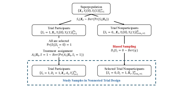
Figure 1: Demonstration of the trial sampling, treatment assignment, and biased sampling in the non-nested design under a superpopulation framework.

Our estimand of interest is the average treatment effect of the target nonparticipants, given by

$$\tau=\mathbb{E}(Y(1)-Y(0)|S=0)$$

To identify the $\tau$, the following assumptions are commonly made (omitting the subscripts):

• : It assumes that, conditional on covariates $X$, the treatment assignment $A$ is independent of the potential outcomes $Y(1)$ and $Y(0)$. It is satisfied by perfectly randomized trials. That is $Y(1),Y(0)\perp A\mid\bm{X},S=1$.

• : It requires that for all values of $\bm{X}$ in the target population, there is a probability of receiving either treatment or control bounding away from 0. That is, there exists a constant $c$ such that $Pr(A=a|\bm{X}=\bm{x},S=1)>c$ for every $a$ and every $x$ with positive density $f_{\bm{X}|S=0}(\bm{x})>0$.

• : It assumes that, conditional on covariates $\bm{X}$, the trial participation is independent of the potential outcomes $Y(1)$ and $Y(0)$. That is $Y(1),Y(0)\perp S\mid\bm{X}$.

• : It requires that for all values of the $\bm{X}$ in the target population, the probability of participating in the trial and observing the outcome is bounded away from 0. That is, there exists a constant $c$ such that $Pr(S=1|\bm{X}=\bm{x})>c$ for every $x$ with positive density $f_{\bm{X}|S=0}(\bm{x})>0$.

• : It assumes no interference between subjects who are selected for the study and those who are not. It also requires treatment version irrelevance between the study and target samples, ensuring consistent treatment across both populations. If $S=1,A=a$, then $Y=Y(a)$.

• : It assumes all trial participants are included in the non-nested design, while only a random subset of the trial nonparticipants is included. That is $Pr(D=1|S=1)=1$, $Pr(D=1|S=0)=Pr(D|S=0,\bm{X},Y(1),Y(0))$, $D\perp(\bm{X},A,Y(1),Y(0))|S$.

2.2 Weighting Estimator and Efficiency Bound

Under the aforementioned assumptions, the $\tau$ can be identified from the observed data. Several estimators have been proposed for its estimation, as reviewed by Li et al. [22]. In this paper, we consider the weighting estimator, which adjusts for unequal probabilities of trial participation and treatment assignment. This approach ensures unbiased estimation by giving more weight to underrepresented observations and reducing the weight for overrepresented ones. A commonly used weighting estimator is the Hájek estimator in survey sampling [23], given by

$$\hat{\tau}_{w}=\frac{\sum_{i=1}^{n}\hat{w}_{1i}Y_{i}}{\sum_{i=1}^{n}\hat{w}_{1i}}-\frac{\sum_{i=1}^{n}\hat{w}_{0i}Y_{i}}{\sum_{i=1}^{n}\hat{w}_{0i}}$$

with estimated weights $w_{ai}$ for $a=0,1$ calculated by

$$w_{a}(S,A,\bm{X};\bm{\alpha},\bm{\beta})=I(S=1,A=a)\frac{(1-h_{s}(\bm{X};\beta))}{h_{s}(\bm{X};\beta)e_{a}(\bm{X};\alpha)}$$

$$\hat{w}_{ai}=w_{a}(S_{i},A_{i},\bm{X};\hat{\bm{\alpha}},\hat{\bm{\beta}})$$

where $I(\cdot)$ is the indicator function; $h_{s}(\bm{X_{i}};\bm{\beta})$ is the trial sampling score condition on study selection modeled by a generalized linear model, and $e_{a}(\bm{X_{i}};\bm{\alpha})$ is the propensity score modeled by a generalized linear model. After applying weighting, the covariates are expected to be balanced between the treatment and control groups and comparable to the distribution of the target population. When both $h_{s}(\bm{X_{i}},\bm{\beta})$ and $e_{a}(\bm{X_{i}},\bm{\alpha})$ are correctly specified, $\hat{\tau}_{w}$ is consistent for $\tau$.

The weighting estimator, while unbiased, is generally not efficient as it does not leverage additional information from the outcome model [24]. To further enhance efficiency, we can estimate the conditional expectation of the outcome using a generalized linear model, denoted as $\mu_{a}(\bm{X};\bm{\theta_{a}})$, and calculate the residuals as

$$R(S,A,Y;\bm{\theta}_{1},\bm{\theta}_{0})=S\{Y-A\mu_{1}(\bm{X};\bm{\theta}_{1})-(1-A)\mu_{0}(\bm{X};\bm{\theta}_{0})\}.$$

The estimated residual is given by

$$\hat{R}_{i}=R(S_{i},A_{i},Y_{i};\hat{\bm{\theta}}_{1},\hat{\bm{\theta}}_{0}),$$

allowing for the use of an augmented weighted estimator:

$$\hat{\tau}_{aw}=\frac{\sum_{i=1}^{n}\hat{w}_{1i}\hat{R}_{i}}{\sum_{i=1}^{n}\hat{w}_{1i}}-\frac{\sum_{i=1}^{n}\hat{w}_{0i}\hat{R}_{i}}{\sum_{i=1}^{n}\hat{w}_{0i}}+\frac{1}{n_{2}}\sum_{i=1}^{n}(1-S_{i})\left\{\mu_{1}(\bm{X}_{i};\hat{\bm{\theta}}_{1})-\mu_{0}(\bm{X}_{i};\hat{\bm{\theta}}_{0})\right\}$$

The augmented weighting estimator is doubly robust, that is when either $h_{s}(\bm{X};\bm{\beta})$ and $e_{a}(\bm{X};\bm{\alpha})$ are correctly specified, or $\mu(a,\bm{X};\bm{\theta}_{a})$ is correctly specified, $\hat{\tau}_{aw}$ is consistent for $\tau$. Even when $\mu(a,\bm{X};\bm{\theta}_{a})$ is misspecified, the augmented weighting estimator can be more efficient than the weighting estimator if the outcome regression model provides reasonable predictions.

Furthermore, under the aforementioned assumptions, the lower bound on the asymptotic variance of any regular estimator for $\tau$ in a semiparametric model can be established [25]. Both the weighting and augmented weighting estimators follow this bound, as they rely on the empirical distribution of $Y$. This bound is given in Theorem 1.

Theorem 2.1.

Under the aforementioned assumptions, the semiparametric efficiency bound for any regular asymptotical linear semiparametric estimator of $\tau$ is

$$V(\tau)=\frac{1}{(1-h_{s})^{2}}\mathbb{E}\left[\left\{\frac{(1-h_{s}(\bm{X}))^{2}}{h_{s}(\bm{X})}\right\}\left(\frac{\sigma_{1}^{2}(\bm{X})}{e_{a}(\bm{X})}+\frac{\sigma_{0}^{2}(\bm{X})}{1-e_{a}(\bm{X})}\right)+(\tau(\bm{X})-\tau)^{2}\right]$$

where $h_{s}$ denotes $Pr(S=1|D=1)$, $\sigma_{1}^{2}(\bm{X})$ denotes $Var(Y(1)|\bm{X},A=1)$, $\sigma_{0}^{2}(\bm{X})$ denotes $Var(Y(0)|\bm{X})$, and $\tau(\bm{X})=\mathbb{E}(Y(1)-Y(0)|\bm{X})$.

Theorem 1 highlights that design factors, such as sampling scores and propensity scores, play a crucial role in determining the semiparametric efficiency bounds. For instance, if, for some $\bm{x}$ with a positive density function $f_{X|S=0}(\bm{x})$, $h_{s}(\bm{x})\to 0$, then $V(\tau)\to\infty$. This implies that challenges at the design stage, such as highly biased sampling or treatment assignment, can result in a large variance bound for any semiparametric estimator. Consequently, this underscores the importance of the positivity assumption and sufficient overlap in ensuring reliable estimation.

3 Proposed Methods for Addressing Positivity Violation

As indicated by Theorem 1, extremely small propensity scores and sampling scores, which can arise from issues at the design stage, lead to unreliable estimation. In fact, the estimator may not even exist if these scores are equal to zero. One common strategy to address this is to shift the focus of estimation to a transportable population[16], which serves as a bridge between the target population and the observed sample. A good transportable population has an acceptable variance in the estimation of its ATE and closely resembles the target population. A widely accepted approach identifies this transportable population as a subset of the target population by excluding subjects with extreme propensity score and sampling score [14, 15]. However, it is important to note that the ATE for the transportable population can differ from that of the original target population.

To address positivity violations when inferring the ATE of the original target population, it is essential to go beyond merely considering the transportable population. Therefore, we propose a novel framework to estimate the ATE of the original target population under conditions of near or full positivity violations. This framework consists of three main steps: (1) dividing the target population into unrepresented, underrepresented, and well-represented groups based on the observed samples; (2) using weighting estimators to estimate the ATE for the well-represented group; and (3) conducting a sensitivity analysis to infer the ATE for the original target population.

3.1 Division of The Target Population

In the first step, we divide individuals within the target population into unrepresented, underrepresented, and well-represented groups, as illustrated in Figure 2. This division is based on the extent to which each group is represented in the observed sample, providing a foundation for subsequent weighting and sensitivity analysis. The three groups are defined as follows:

• Unrepresented Group $\mathcal{R}_{1}$: This group includes individuals for whom no comparable subjects were observed in the study sample, either because their trial participation probability is zero, $h_{s}(\bm{X})=0$, or because they lack comparable subjects in the opposite treatment group, i.e., $e_{a}(\bm{X})=0$ or $1-e_{a}(\bm{X})=0$. Formally, this group is defined as $\mathcal{R}_{1}=\{\bm{X}\in\mathcal{X}_{\text{excl}}\}$, where $\mathcal{X}_{\text{excl}}$ represents the region of the covariate space for these subjects, determined by the trial inclusion criteria and treatment assignment rules.

• Underrepresented Group $\mathcal{R}_{2}$: This group includes individuals for whom the sampling score or the propensity score for one treatment is extremely small. It is defined as $\mathcal{R}_{2}=\{\bm{X}\mid h_{s}(\bm{X})e_{a}(\bm{X})<\delta\text{ and }h_{s}(\bm{X})(1-e_{a}(\bm{X}))<\delta,\text{ and }\bm{X}\notin\mathcal{X}_{\text{excl}}\}$, where $\delta$ is a small threshold value indicating extreme underrepresentation.

• Well-Represented Group $\mathcal{R}_{3}$: This group includes individuals for whom the sampling score and propensity score for both treatments are not extremely small, ensuring adequate representation. It is defined as $\mathcal{R}_{3}=\{\bm{X}\mid\bm{X}\notin\mathcal{R}_{1}\cup\mathcal{R}_{2}\}$.

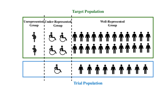
Figure 2: Demonstration of the division of the target population based on patients’ characteristics.

Accordingly, the ATE for the target population can be expressed as a weighted sum of the ATEs for each group:

$$\tau=p_{1}\tau_{1}+p_{2}\tau_{2}+p_{3}\tau_{3}=(1-p_{3})\tau_{12}+p_{3}\tau_{3},$$

where $\tau_{j}=\mathbb{E}(Y(1)-Y(0)\mid\bm{X}\in\mathcal{R}_{j},S=0)$, and $p_{j}$ for $j=1,2,3$ represents the proportion of each corresponding group in the target population. Additionally, $\tau_{12}=\mathbb{E}(Y(1)-Y(0)\mid\bm{X}\in\mathcal{R}_{1}\cup\mathcal{R}_{2},S=0)$.

In this division, the groups $\mathcal{R}_{1}$ and $\mathcal{R}_{2}$ need to be separated because the sampling or propensity scores for individuals in $\mathcal{R}_{1}$ are exactly zero due to the study’s inclusion criteria and strict treatment assignment rules. This means that their scores do not require estimation, and their ATE is unidentifiable. Additionally, imputing outcomes for $\mathcal{R}_{1}$ requires extra assumptions through statistical modeling, as outcomes for individuals in $\mathcal{R}_{1}$ are not observed. This challenge is particularly relevant when the rules defining $\mathcal{R}_{1}$ involve categorical variables [17]. Furthermore, $\mathcal{R}_{2}$ and $\mathcal{R}_{3}$ must also be separated because subjects in $\mathcal{R}_{2}$ disproportionately inflate the variance in ATE estimation, as indicated by Theorem 2.1. This separation allows us to identify a subset of the target population—the well-represented group—that can be efficiently estimated while also enabling investigators to better report the limitations of their study sample.

However, determining an appropriate threshold $\delta$ to separate $\mathcal{R}_{2}$ and $\mathcal{R}_{3}$ is often challenging. To address this, we propose defining $\delta$ based on the desired proportion of subjects to retain in the well-represented group for inference, similar to trimming based on quantiles [26, 27, 28]. This approach offers several advantages: it allows flexibility in controlling the proportion of data retained, helping to balance estimation efficiency and robustness. It is adaptable to various data distributions and does not rely on distributional assumptions, making it a practical choice when external information is limited. Finally, the concept of being “well-represented” is inherently relative, as the over-representation of some groups leads to the under-representation of others, making a proportion or quantile-based approach a logical choice to account for these imbalances.

To facilitate later estimation, the membership in $\mathcal{R}_{3}$ is defined by the inclusion weight

$$\mathcal{R}_{3}=\{\bm{X}\mid k(\bm{X};\delta)=1\},$$

$$k(\bm{X};\delta)=I(h_{s}(\bm{X})e_{a}(\bm{X})\geq\delta)I((1-e_{a}(\bm{X}))h_{s}(\bm{X})\geq\delta).$$

If the desired proportion of well-represented subjects is $p_{3}^{*}$, the threshold $\delta^{*}$ is chosen to satisfy the following condition:

$$\mathbb{E}(k(\bm{X};\delta^{*})\mid S=0)=p_{3}^{*}.$$

Since $\delta^{*}$ must be estimated from the data, we suggest employing a smooth inclusion function, as proposed by Yang and Ding [29], which allows for conventional asymptotic linearization techniques to analyze the resulting estimators. Specifically, we define the smooth inclusion function as

$$k_{s}(\bm{X};\delta,\epsilon,\bm{\alpha},\bm{\beta})=\Phi_{\epsilon,\delta}(h_{s}(\bm{X};\bm{\beta})e_{a}(\bm{X};\bm{\alpha}))\Phi_{\epsilon,\delta}(h_{s}(\bm{X};\bm{\beta})(1-e_{a}(\bm{X};\bm{\alpha}))),$$

where $\Phi_{\epsilon,\delta}(\cdot)$ represents the cumulative distribution function of a normal distribution with mean $\delta$ and a fixed variance $\epsilon^{2}$ (e.g. $\epsilon=10^{-8}$). The smooth function $k_{s}(\bm{X};\delta,\epsilon)$ approaches the original indicator-based function $k(\bm{X};\delta)$ as $\epsilon\to 0$.

Accordingly, the smooth inclusion weight for observed subjects, based on the estimated propensity score and sampling score, is given by

$$\hat{k}_{si}(\delta)=\Phi_{\epsilon,\delta}(h_{s}(\bm{X};\hat{\bm{\beta}})e_{a}(\bm{X};\hat{\bm{\alpha}}))\Phi_{\epsilon,\delta}(h_{s}(\bm{X};\hat{\bm{\beta}})(1-e_{a}(\bm{X};\hat{\bm{\alpha}}))).$$

3.2 Inference in Well-Represented Group

After dividing the target population into three groups, the inference for the well-represented group can be obtained using the aforementioned Hájek weighting estimator or the augmented weighting estimator with additional defined inclusion weights.

Specifically, the required parameter $\bm{\Xi}_{w}=[\bm{\beta},\bm{\alpha},\delta^{*},\mu_{31},\mu_{30}]^{T}$ for the weighting estimator is obtained by solving the estimating equation

$$\sum_{i=1}^{n}\bm{\Psi}_{w}(S_{i},\bm{X}_{i},A_{i},Y_{i};\hat{\bm{\Xi}}_{w})=0,$$

where the estimating function $\bm{\Psi}_{w}(S,\bm{X},A,Y;\bm{\Xi}_{w})$ is defined as

$$\bm{\Psi}_{w}(S,\bm{X},A,Y;\bm{\Xi}_{w})=\begin{bmatrix}\bm{\Psi}_{\bm{\beta}}\\ \bm{\Psi}_{\bm{\alpha}}\\ \Psi_{\delta^{*}}\\ \Psi_{\mu_{30}}\\ \Psi_{\mu_{31}}\\ \end{bmatrix}=\begin{bmatrix}\{S-h_{1}(\bm{X}^{T}\bm{\beta})\}\bm{X}\\ S\{A-h_{1}(\bm{X}^{T}\bm{\alpha})\}\bm{X}\\ (1-S)k_{s}(\bm{X};\delta,\epsilon,\bm{\alpha},\bm{\beta})-p_{3}^{*}\\ k_{s}(\bm{X};\delta,\epsilon,\bm{\alpha},\bm{\beta})w_{1}(S,A,\bm{X};\bm{\alpha},\bm{\beta})(Y-\mu_{31})\\ k_{s}(\bm{X};\delta,\epsilon,\bm{\alpha},\bm{\beta})w_{0}(S,A,\bm{X};\bm{\alpha},\bm{\beta})(Y-\mu_{30})\\ \end{bmatrix}.$$

where $\bm{\Psi}_{\bm{\beta}}$ and $\bm{\Psi}_{\bm{\alpha}}$ are the score function vectors for the sampling score and propensity score models, respectively, with $h_{1}(\cdot)$ as the link function. $\Psi_{\mu_{30}}$ and $\Psi_{\mu_{31}}$ represent the estimating functions for the mean outcomes in the control and treatment groups within the well-represented group. And the weighting estimator for well-represented group $\hat{\tau}_{3w}$ is given by

$$\hat{\tau}_{3w}=\hat{\mu}_{31}-\hat{\mu}_{30}$$

Similarly, the required parameter $\bm{\Psi}_{aw}(S,\bm{X},A,Y;\bm{\Xi}_{aw})$ is is obtained by the estimating equation

$$\sum_{i=1}^{n}\bm{\Psi}_{aw}(S_{i},\bm{X},A,Y;;\hat{\bm{\Xi}}_{aw})=0$$

where the estimating function $\bm{\Psi}_{w}(S,\bm{X},A,Y;\bm{\Xi}_{w})$ is defined as

$$\bm{\Psi}_{aw}(S,\bm{X},A,Y;\bm{\Xi}_{aw})=\begin{bmatrix}\bm{\Psi}_{\bm{\beta}}\\ \bm{\Psi}_{\bm{\alpha}}\\ \Psi_{\bm{\theta}_{1}}\\ \Psi_{\bm{\theta}_{0}}\\ \Psi_{\delta^{*}}\\ \Psi_{v_{1}}\\ \Psi_{v_{2}}\\ \Psi_{v_{3}}\end{bmatrix}=\begin{bmatrix}\{S-h_{1}(\bm{X}^{T}\bm{\beta})\}\bm{X}\\ S\{A-h_{1}(\bm{X}^{T}\bm{\alpha})\}\bm{X}\\ SA_{i}\{Y_{i}-h_{2}(\bm{X}^{T}\bm{\theta}_{1})\}\bm{X}\\ S(1-A_{i})\{Y_{i}-h_{2}(\bm{X}^{T}\bm{\theta}_{0})\}\bm{X}\\ (1-S)k_{s}(\bm{X};\delta,\epsilon,\bm{\alpha},\bm{\beta})-p_{3}^{*}\\ k_{s}(\bm{X};\delta,\epsilon,\bm{\alpha},\bm{\beta})w_{1}(S,A,\bm{X};\bm{\alpha},\bm{\beta})\{R(S,A,Y;\bm{\theta}_{0},\bm{\theta}_{1})-v_{1}\}\\ k_{s}(\bm{X};\delta,\epsilon,\bm{\alpha},\bm{\beta})w_{0}(S,A,\bm{X};\bm{\alpha},\bm{\beta})\{R(S,A,Y;\bm{\theta}_{0},\bm{\theta}_{1})-v_{2}\}\\ k_{s}(\bm{X};\delta,\epsilon,\bm{\alpha},\bm{\beta})(1-S)\{\mu_{1}(\bm{X};\bm{\theta}_{1})-\mu_{0}(\bm{X};\bm{\theta}_{0})-v_{3}\}\\ \end{bmatrix}$$

where $\bm{\Psi}_{\bm{\theta}_{1}}$ and $\bm{\Psi}_{\bm{\theta}_{0}}$ are the score function vectors for the outcome regression in the treatment and control groups, respectively, and $h_{2}(\cdot)$ is the link function for their generalized model. $\bm{\Psi}_{v_{1}}$ and $\bm{\Psi}_{v_{2}}$ are the estimating functions for the weighted average residuals in the treatment and control groups. $\bm{\Psi}_{v_{3}}$ represents the estimating function for the ATE based on the outcome regression. And the augmented weighting estimator for well-represented group $\hat{\tau}_{3aw}$ is given by

$$\hat{\tau}_{3aw}=\hat{v}_{1}-\hat{v}_{2}+\hat{v}_{3}$$

For the two proposed estimators, the following theorems are established using the M-estimation theory and the delta method to support their inference.

Theorem 3.1.

$\hat{\tau}_{3w}$ is asymptotically linear. Furthermore,

$$\frac{1}{\sqrt{n}}(\hat{\tau}_{3w}-\tau_{3})\rightarrow N(0,\bm{\eta}_{w}^{T}\bm{A}_{w}^{-1}\bm{B}_{w}\bm{A}_{w}^{-T}\bm{\eta}_{w})$$

where

$$\bm{A}_{w} =\mathbb{E}\left(\frac{\partial}{\partial\bm{\Xi}_{w}^{T}}\Psi_{w}(S_{i},\bm{X}_{i},A_{i},Y_{i})\right),$$

$$\bm{B}_{w} =\mathbb{E}\left(\Psi_{w}(S_{i},\bm{X}_{i},A_{i},Y_{i})\Psi_{w}^{T}(S_{i},\bm{X}_{i},A_{i},Y_{i})\right),$$

$$\bm{\eta}_{w} =[\bm{0}_{1\times p},\bm{0}_{1\times p},0,1,-1].$$

Theorem 3.2.

$\hat{\tau}_{3aw}$ is asymptotically linear. Furthermore,

$$\frac{1}{\sqrt{n}}(\hat{\tau}_{3aw}-\tau_{3})\rightarrow N(0,\bm{\eta}_{aw}^{T}\bm{A}_{aw}^{-1}\bm{B}_{aw}\bm{A}_{aw}^{-T}\bm{\eta}_{aw}),$$

where

$$\bm{A}_{aw} =\mathbb{E}\left(\frac{\partial}{\partial\bm{\Xi}_{aw}^{T}}\Psi_{aw}(S_{i},\bm{X}_{i},A_{i},Y_{i})\right),$$

$$\bm{B}_{aw} =\mathbb{E}\left(\Psi_{aw}(S_{i},\bm{X}_{i},A_{i},Y_{i})\Psi_{aw}^{T}(S_{i},\bm{X}_{i},A_{i},Y_{i})\right),$$

$$\bm{\eta}_{aw} =[\bm{0}_{1\times p},\bm{0}_{1\times p},\bm{0}_{1\times p},\bm{0}_{1\times p},0,1,-1,1].$$

The above theorems indicate that the variance for the proposed weighting estimator based on the smooth inclusion weights under the estimated threshold can be estimated using either bootstrapping or a sandwich variance estimator.

3.3 Inference in Target Population

Building on the estimation in the well-represented group, we now extend the inference to the target population. Since direct inference from observed data for unrepresented and underrepresented groups is either infeasible or highly variable, we propose estimating the ATE for these groups using a sensitivity parameter under two distinct assumptions.

In the first approach, we infer the ATE for unrepresented and underrepresented groups by assuming a proportional difference relative to the well-represented group. Specifically:

• The ATE for the unrepresented and underrepresented groups is assumed to be $k$ times the ATE of the well-represented group, i.e., $\tau_{12}=k\tau_{3}$.

Thus, the overall estimated ATE is

$$\hat{\tau}=(1-p_{3}^{*})\hat{\tau}_{12}+p_{3}^{*}\hat{\tau_{3}}=(1-p_{3}^{*})k\hat{\tau}_{3}+p_{3}^{*}\hat{\tau_{3}}$$

Furthermore,

$$\frac{1}{\sqrt{n}}(\hat{\tau}-\tau)\rightarrow N(0,(k(1-p_{3}^{*})+p_{3}^{*})^{2}V_{3})$$

where $V_{3}$ is the asymptotical variance of $\frac{1}{\sqrt{n}}(\hat{\tau_{3}}-\tau_{3})$. When $k=1$, we assume that there is no difference between the ATE of well-represented groups and the ATE of unrepresented and underrepresented groups. The influence of the unrepresented and underrepresented groups is determined by two factors: (1) the proportion of subjects in these groups and (2) and proportional difference between the groups.

The second approach relies on the extrapolation of $\tau_{12}$ using either a statistical or mathematical model.

Let

$$\zeta_{12}=\frac{1}{n(1-p_{3}^{*})}\sum_{i:\bm{X}_{i}\in\mathcal{R}_{1}\cup\mathcal{R}_{2}}\left(m(1,\bm{X}_{i})-m(0,\bm{X}_{i})\right)$$

where $m(a,\bm{X}_{i})$ can represent a statistical model, such as an outcome model [30, 31], a propensity score model [32], or a mathematical model specified by the investigator [17, 18]. Notably, when an unrepresented group arises due to a categorical variable, incorporating a mathematical model or additional model assumptions is essential.

We make the following assumption:

• : The ATE for the unrepresented and underrepresented groups is assumed to be $k$ times their model-based extrapolation result, i.e., $\tau_{12}=k\zeta_{12}$.

Thus, the overall estimated ATE is given by

$$\hat{\tau}=(1-p_{3}^{*})\tau_{12}+p_{3}^{*}\hat{\tau}_{3}=(1-p_{3}^{*})k\zeta_{12}+p_{3}^{*}\hat{\tau}_{3}$$

Furthermore,

$$\frac{1}{\sqrt{n}}(\hat{\tau}-\tau)\rightarrow N\left(0,{p_{3}^{*}}^{2}V_{3}\right)$$

The sensitivity parameter $k$ is introduced for extrapolation results because both the point estimate and uncertainty quantification are highly influenced by model specifications for underrepresented or unrepresented groups. Mathematical models specified by the investigator do not inherently ensure accuracy. Moreover, statistical model extrapolation is reliable only when no unrepresented groups exist, and the outcome model is parametrically specified correctly. Under these conditions, the ATE from extrapolation converges to the true value at a rate of $\sqrt{n}$. However, if the model is misspecified, a semiparametric model is applied, or unrepresented groups are present, the asymptotic distribution of $\hat{\tau}$ can be negatively affected. Under this sensitivity approach, the impact of underrepresented and unrepresented groups depends on three factors: the proportion of subjects in these groups, the extrapolation result, and the proportional difference between the extrapolation result and true ATE of unrepresented and underrepresented groups.

Following these three steps enables us to assess the trial sampling mechanism across the three groups, make the inference in the well-represented group, and examine the robustness of the findings for the entire target population through sensitivity analysis.

4 Simulation Study

In this section, we conducted simulation studies to evaluate the finite-sample performance of the proposed methods. For inference, we assumed the sensitivity parameter to be known. Specifically, in the first approach, we assumed that the proportional differences between groups were known, while in the second approach, we assumed that the ATE for unrepresented or underrepresented groups was known. Based on these assumptions, we evaluated the mean bias, mean squared error, standard deviation, and coverage rate of the proposed estimators across 1,000 replications.

4.1 Data Generation

We simulated cohorts with total sample sizes of $\tilde{n}=20000$, $50000$, and $100000$ individuals, with corresponding trial sample sizes $n_{1}$ of approximately 200, 500, and 1000. Specifically, we generated baseline covariates $\bm{X_{i}}=(1,X_{1i},X_{2i},X_{3i})$, where $X_{ji}\sim N(0,1)$ for $j=1,2,3$. Additionally, we included a binary covariate $E\sim Ber(0.01)$, which strictly excludes individuals from the trial when $E=1$. Selection into the trial was simulated using a binary indicator $S_{i}$, where $\Pr[S=1|\bm{X},E=1]=\frac{1}{1+\exp(-\bm{X}^{\top}\bm{\beta})}$ with $\bm{\beta}=[-5.974121,-5,1,1]$, and $\Pr[S=1|E=0]=0$. We chose intercept of in $\bm{\beta}$ using numerical methods [33], such that the trial participation probability is 1%. We then randomly sampled 10% of the non-participants as observed samples with baseline covariates for nonparticipants. The sample size of selected non-participants $n_{2}$ is approximately 1980, 4950, and 9990. Potential outcomes were generated as $Y(a)\sim N(\bm{X}^{\top}\bm{\theta}_{a})$, with $\bm{\theta}_{0}=[1,2,2,1]$ and $\bm{\theta}_{1}=[0,1,1,1]$. For trial participants, we generated treatment assignment $A$, where $A\sim\text{Bernoulli}(0.5)$. The observed outcome for trial participants ($S_{i}=1$) is $Y_{i}=AY_{i}+(1-A)Y_{i}$.

For the simulated dataset across three sample size settings, we estimated the well-represented group proportions at $90\%$ and $80\%$ using both the weighting and augmented weighting estimators. Subsequently, inference for the original target population was conducted with known sensitivity parameters using each of the two approaches. This setup resulted in a total of 8 estimators for each sample size setting.

4.2 Simulation Result

Tables 1 present simulation results for eight estimators across three different sample size settings. All estimators are unbiased and consistently converge to the true value as the sample size increases, with coverage rates reaching nominal levels in larger samples. Among the estimators, the augmented weighting estimator consistently demonstrated lower bias, mean squared error (MSE), and variability compared to the standard weighting estimator, indicating superior performance in terms of precision and reliability. However, in this setup, the augmented weighting estimator is no longer doubly robust, as the classification of subjects into the well-represented group depends on estimated sampling scores and propensity scores.

Efficiency gains were observed in both estimators when the proportion of well-represented groups was 0.8, compared to 0.9, suggesting that the methods perform better when a larger proportion of subjects with low sampling probability are excluded in our simulation setting. However, determining the optimal proportion for efficiency gains in a real-world setting remains challenging. Chen et al. [14] proposed selecting the proportion that minimizes the estimated efficiency bound. However, the asymptotic behavior of this approach is unknown when the well-represented group is defined by minimizing the estimated efficiency bound based on the estimated scores. Furthermore, the improvement in efficiency assumes that the sensitivity parameter is known and remains constant throughout the simulations. When the sensitivity parameter is unknown, its impact becomes more substantial, particularly when the proportion of well-represented groups is lower. This introduces a trade-off between efficiency gains and the influence of the sensitivity parameter in the later stages of sensitivity analysis.

Additionally, under the group proportional difference assumption, there is a smaller bias, mean squared error (MSE), and variability in our setting compared to the extrapolation proportional difference assumption. However, this result relies on the assumption that the sensitivity parameter is known, which is not feasible in practice. In real-world applications, both assumptions are worth considering when addressing positivity violations, as each provides valuable insights depending on the specific context and available data.

Table 1: Simulation Results. This table presents simulation results for various trial and target sizes, comparing two methods (IPW and AIPW) under two assumptions (EPD and GPD) and across different proportions of well-represented groups.

Trial Size	Target Size	Proportion	Method	Assumption	Bias	MSE	SD	Coverage
200	1980	0.8	IPW	EPD	-0.046	0.280	0.528	0.924
200	1980	0.8	IPW	GPD	-0.041	0.225	0.473	0.924
400	4950	0.8	IPW	EPD	-0.016	0.109	0.331	0.958
400	4950	0.8	IPW	GPD	-0.014	0.088	0.296	0.958
1000	9990	0.8	IPW	EPD	-0.012	0.054	0.233	0.961
1000	9990	0.8	IPW	GPD	-0.010	0.044	0.209	0.961
200	1980	0.8	AIPW	EPD	0.002	0.042	0.206	0.948
200	1980	0.8	AIPW	GPD	0.002	0.034	0.184	0.948
400	4950	0.8	AIPW	EPD	-0.002	0.015	0.124	0.952
400	4950	0.8	AIPW	GPD	-0.002	0.012	0.111	0.951
1000	9990	0.8	AIPW	EPD	-0.004	0.008	0.090	0.945
1000	9990	0.8	AIPW	GPD	-0.004	0.006	0.080	0.945
200	1980	0.9	IPW	EPD	-0.103	0.611	0.775	0.897
200	1980	0.9	IPW	GPD	-0.095	0.515	0.712	0.897
400	4950	0.9	IPW	EPD	-0.037	0.271	0.519	0.919
400	4950	0.9	IPW	GPD	-0.034	0.228	0.477	0.919
1000	9990	0.9	IPW	EPD	-0.043	0.133	0.362	0.950
1000	9990	0.9	IPW	GPD	-0.040	0.112	0.332	0.950
200	1980	0.9	AIPW	EPD	0.001	0.062	0.250	0.940
200	1980	0.9	AIPW	GPD	0.001	0.053	0.229	0.940
400	4950	0.9	AIPW	EPD	-0.003	0.023	0.151	0.948
400	4950	0.9	AIPW	GPD	-0.003	0.019	0.139	0.948
1000	9990	0.9	AIPW	EPD	-0.006	0.012	0.109	0.946
1000	9990	0.9	AIPW	GPD	-0.005	0.010	0.100	0.946

• Abbreviations: IPW, Inverse Probability Weighting; AIPW, Augmented IPW; EPD, Estimated Propensity Difference; GPD, Generalized Propensity Difference.

5 Application

Opioid use disorder is a serious condition that increases the risk of overdose, relapse, and significant physical, mental, and social harm if left untreated. Medication-assisted treatments, such as buprenorphine (BUP) and methadone (MET), are among the most effective options for managing this disorder. However, treatment success often depends on patient adherence to the prescribed regimen, with nonadherence leading to suboptimal outcomes. To assess the effectiveness of these treatments, the Starting Treatment with Agonist Replacement Therapy (START) trial, a multi-center study, randomized 1,271 participants in a 2:1 ratio to receive either BUP or MET. A secondary analysis of the trial data indicated that MET had significantly higher treatment completion rates than BUP, with 74% of MET participants completing treatment compared to 46% of BUP participants (p < 0.01) [34].

To generalize these findings to a broader real-world population, we used data from the 2021 Treatment Episode Data Set – Admissions (TEDS-A), which includes 166,270 individuals receiving medication-assisted treatment for opioid dependence or abuse. Table 2 compares the baseline covariates of the START trial sample with those of the TEDS-A population. Our primary goal was to estimate the average treatment effect of BUP versus MET on treatment completion rates in the real-world population. However, positivity violations were observed due to age and pregnancy exclusions in the trial sample, as well as baseline covariates that influenced trial participation.

Two logistic regression models—one for treatment assignment and another for trial participation—were constructed to evaluate the trial design. Both models included covariates such as age, sex, race, injection behavior, other substance use, and two-way interactions involving race. While treatment assignment was unbiased due to randomization, trial participation exhibited selection bias. Figure 3 presents the distribution of estimated probabilities of trial participation for the START trial participants and the TEDS-A population. Compared to the START trial participants, a larger proportion of individuals in the TEDS-A population had extremely low or zero probabilities of participating in the trial. Using the estimated propensity and sampling scores, the target TEDS-A population was divided into three groups based on the trial exclusion criteria, with the well-represented group defined as comprising 90% of the total target population.

Table 2: Baseline Characteristics of Study Sample and Target Population. This table presents baseline characteristics comparing the Buprenorphine/Naloxone group, the Methadone group in the trial, and the Target Population.

Characteristic	Buprenorphine/Naloxone	Methadone	Target Population
Sample Size	654	440	166,270
Age, years
12-14	0 (0.0%)	0 (0.0%)	4 (0.0%)
15-17	0 (0.0%)	0 (0.0%)	88 (0.1%)
18-20	14 (2.1%)	2 (0.5%)	1,827 (1.1%)
21-24	76 (11.6%)	52 (11.8%)	7,873 (4.7%)
25-29	122 (18.7%)	88 (20.0%)	25,499 (15.3%)
30-34	96 (14.7%)	67 (15.2%)	36,147 (21.7%)
35-39	71 (10.9%)	40 (9.1%)	29,558 (17.8%)
40-44	69 (10.6%)	58 (13.2%)	20,724 (12.5%)
45-49	88 (13.5%)	57 (13.0%)	12,785 (7.7%)
50-54	66 (10.1%)	49 (11.1%)	11,768 (7.1%)
55-64	50 (7.6%)	25 (5.7%)	16,063 (9.7%)
65+	2 (0.3%)	2 (0.5%)	3,934 (2.4%)
Male	451 (69.0%)	300 (68.2%)	105,980 (63.7%)
Pregnancy
Yes	0 (0.0%)	0 (0.0%)	2,980 (1.8%)
No	203 (31.0%)	140 (31.8%)	57,310 (34.5%)
Not applicable	451 (69.0%)	300 (68.2%)	105,980 (63.7%)
Race
White	433 (66.2%)	308 (70.0%)	108,176 (65.1%)
Hispanic	107 (16.4%)	63 (14.3%)	28,609 (17.2%)
Black	59 (9.0%)	40 (9.1%)	20,385 (12.3%)
Other	55 (8.4%)	29 (6.6%)	9,100 (5.5%)
Substance Use
Injection drug use	441 (67.4%)	306 (69.5%)	77,319 (46.5%)
Alcohol use	141 (21.6%)	110 (25.0%)	21,343 (12.8%)
Amphetamines use	70 (10.7%)	50 (11.4%)	27,934 (16.8%)
Cannabis use	124 (19.0%)	99 (22.5%)	24,698 (14.9%)
Sedatives use	94 (14.4%)	59 (13.4%)	13,342 (8.0%)
Cocaine use	206 (31.5%)	151 (34.3%)	41,174 (24.8%)
Completed Study	303 (46.3%)	325 (73.9%)	-

• Abbreviations: Percentages are shown in parentheses for each characteristic.

• Note: "Not applicable" refers to characteristics irrelevant to certain groups (e.g., pregnancy for males).

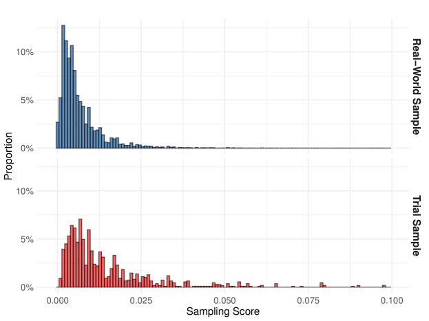
Figure 3: Histogram of sampling score in STAR trial and 2021 TEA data

• Unrepresented Group (3,071; 2%): Individuals excluded by trial criteria, including those under 18 years old or pregnant.

• Underrepresented Group (13,487; 8%): Individuals with extreme weights. This group includes:

  • Black individuals aged 55-64 years who do not depend on other drugs and do not use injection drugs (4,456).

  • Black males aged 18-20, 30-34, or 65 years and older who do not depend on other drugs and do not use injection drugs (1,164).

  • Hispanic or Black males aged 35-39 years who do not depend on other drugs and do not use injection drugs (1,108).

  • White or Hispanic individuals aged 35-39 years who depend on amphetamines and do not use injection drugs (1,101).

  • Black females aged 30-34, 35-39, 40-44, or 65 years and older who do not depend on other drugs and do not use injection drugs (955).

  • White, Hispanic, or individuals of other races aged 65 years and older who do not depend on other drugs and do not use injection drugs (842).

  • Black males aged 18-20, 25-29, 30-34, 35-39, 40-44, 45-49, 50-54, or 65 years and older who depend on cannabis and use injection drugs (644).

  • Other individuals (5,421).

• Well-represented Group (149,712; 90%): Individuals who do not belong to either of the above groups.

For the well-represented group in the target population, the ATE is 26.4% (95% CI [19.6%–33.1%]) based on the augmented weighting estimator. Two sensitivity analysis approaches were applied to address the original question. In both approaches, the sensitivity parameter was varied within a range of -2 to 2. A 10% increase in the completion rate is considered clinically meaningful. Based on the Figure 4. The findings from the sensitivity analyses demonstrated a reasonable level of robustness, maintaining their significance within the specified parameter range.

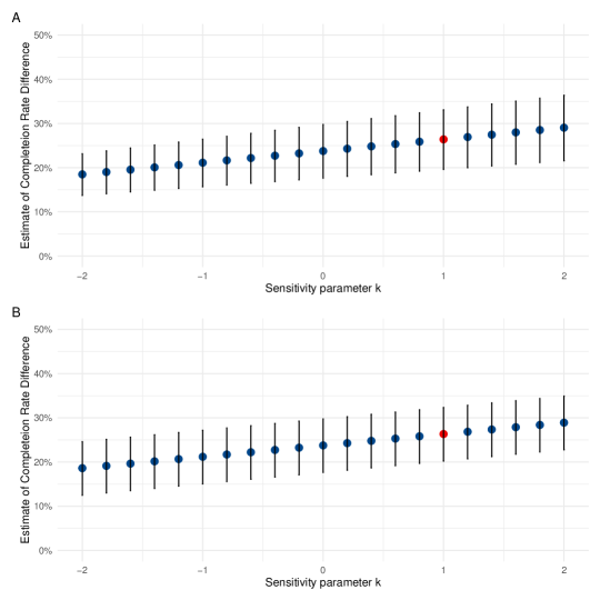
Figure 4: Sensitivity analyses for the average treatment effect on completion rates: (A) Group Proportional Difference (B) Extrapolation Proportional Difference. The red point estimate is corresponding to $k=1$.

6 Disscusion

In this paper, we propose an integrative framework to address positivity violations when estimating the ATE of a target population. After performing positivity checks and calculating the sampling and propensity scores, the target population is divided into three parts. The well-represented portion is inferred with confidence, while the remaining two parts are inferred with the help of a sensitivity parameter. This approach combines positivity checking, trimming, and sensitivity analysis into a unified framework.

A variety of methods are available for determining the separation threshold for trimming or truncation when addressing violations of the positivity assumption. In addition to quantile-based and fixed threshold criteria, the separation threshold can also be set by minimizing the efficiency bound [14, 15, 35, 36], proximal mean squared error [37], or asymptotic mean squared error [32]. However, the asymptotic properties when minimizing the efficiency bound are only guaranteed when the uncertainty in estimating the threshold is ignored. In other words, this criterion defines the estimand of the ATE based on well-represented groups within each version of the observed samples, rather than the true underlying data-generating process. Meanwhile, minimizing the proximal mean squared error lacks any established asymptotic theory. Ma and Wang [32] established the asymptotic behavior of estimation under minimizing the asymptotic mean squared error criterion, and extending this approach to settings involving a target population would be valuable. Our sensitivity analysis remains compatible with group division using these methods. We prefer to incorporate the uncertainty in group division and control the introduced bias by chosen proportion, which is why we choose quantile-based criteria. In practice, researchers may wish to assess the ATE for well-represented groups at different proportions and check the trade-off of trimmed proportion and gained efficiency. One practical approach is to perform simultaneous inference across a set of proportions, as suggested by Khan and Ugander [36].

In addition to identifying the transportable population as a subset of the target population, entropy weighting and its modifications have been proposed as alternatives that identify the transportable population using moment constraints to align the mean or other aspects of the covariate distribution [38, 39]. However, entropy weighting relies on untestable parametric assumptions about the outcome given the covariates. These additional assumptions also necessitate other corresponding sensitivity analyses to assess their robustness.

In the future, we aim to extend our framework to handle ordinal or continuous treatments, where positivity violations are more likely to occur. Additionally, we plan to integrate semiparametric models into the estimation of propensity scores, sampling scores, and outcome regressions, as these models offer greater flexibility.

References

- Kim et al. [2017] Kim ES, Bruinooge SS, Roberts S, Ison G, Lin NU, Gore L, et al. Broadening eligibility criteria to make clinical trials more representative: American Society of Clinical Oncology and Friends of Cancer Research Joint Research Statement. Journal of Clinical Oncology 2017;35(33):3737–3744.
- Nguyen et al. [2023] Nguyen RH, Silva Y, Lu J, Chen Z, Gadi V. Race and Ethnicity Reporting and Enrollment Disparities in Clinical Trials Leading to FDA Approvals for Breast Cancer Between 2010 and 2020. Clinical Breast Cancer 2023;23(6):591–597.
- FDA [2019] FDA, Enhancing the Diversity of Clinical Trial Populations — Eligibility Criteria, Enrollment Practices, and Trial Designs: Guidance for Industry; 2019. https://www.fda.gov/media/127712/download, accessed: 2024-11-18.
- Ling et al. [2023] Ling AY, Montez-Rath ME, Carita P, Chandross KJ, Lucats L, Meng Z, et al. An overview of current methods for real-world applications to generalize or transport clinical trial findings to target populations of interest. Epidemiology 2023;34(5):627–636.
- Dahabreh et al. [2019] Dahabreh IJ, Robertson SE, Tchetgen EJ, Stuart EA, Hernán MA. Generalizing causal inferences from individuals in randomized trials to all trial-eligible individuals. Biometrics 2019;75(2):685–694.
- Dahabreh et al. [2020] Dahabreh IJ, Robertson SE, Steingrimsson JA, Stuart EA, Hernan MA. Extending inferences from a randomized trial to a new target population. Statistics in medicine 2020;39(14):1999–2014.
- Lesko et al. [2016] Lesko CR, Cole SR, Hall HI, Westreich D, Miller WC, Eron JJ, et al. The effect of antiretroviral therapy on all-cause mortality, generalized to persons diagnosed with HIV in the USA, 2009–11. International journal of epidemiology 2016;45(1):140–150.
- Nguyen et al. [2017] Nguyen TQ, Ebnesajjad C, Cole SR, Stuart EA. Sensitivity analysis for an unobserved moderator in RCT-to-target-population generalization of treatment effects. The Annals of Applied Statistics 2017;p. 225–247.
- Nguyen et al. [2018] Nguyen TQ, Ackerman B, Schmid I, Cole SR, Stuart EA. Sensitivity analyses for effect modifiers not observed in the target population when generalizing treatment effects from a randomized controlled trial: Assumptions, models, effect scales, data scenarios, and implementation details. PloS one 2018;13(12):e0208795.
- Steingrimsson et al. [2023] Steingrimsson JA, Robertson SE, Dahabreh IJ. Sensitivity analysis for studies transporting prediction models. arXiv preprint arXiv:230608084 2023;.
- Dahabreh et al. [2023] Dahabreh IJ, Robins JM, Haneuse SJP, Saeed I, Robertson SE, Stuart EA, et al. Sensitivity analysis using bias functions for studies extending inferences from a randomized trial to a target population. Statistics in Medicine 2023;42(13):2029–2043.
- Huang [2024] Huang MY. Sensitivity analysis for the generalization of experimental results. Journal of the Royal Statistical Society Series A: Statistics in Society 2024;p. qnae012.
- Nilsson et al. [2023] Nilsson A, Björk J, Bonander C. Proxy variables and the generalizability of study results. American Journal of Epidemiology 2023;192(3):448–454.
- Chen et al. [2023] Chen R, Chen G, Yu M. A generalizability score for aggregate causal effect. Biostatistics 2023;24(2):309–326.
- Parikh et al. [2024] Parikh H, Ross R, Stuart E, Rudolph K. Who are we missing? a principled approach to characterizing the underrepresented population. arXiv preprint arXiv:240114512 2024;.
- Huang [2024] Huang M. Overlap violations in external validity. arXiv preprint arXiv:240319504 2024;.
- Zivich et al. [2023] Zivich PN, Edwards JK, Shook-Sa BE, Lofgren ET, Lessler J, Cole SR. Synthesis estimators for positivity violations with a continuous covariate. arXiv preprint arXiv:231109388 2023;.
- Zivich et al. [2024] Zivich PN, Edwards JK, Lofgren ET, Cole SR, Shook-Sa BE, Lessler J. Transportability without positivity: a synthesis of statistical and simulation modeling. Epidemiology 2024;35(1):23–31.
- Dahabreh et al. [2021] Dahabreh IJ, Haneuse SJA, Robins JM, Robertson SE, Buchanan AL, Stuart EA, et al. Study designs for extending causal inferences from a randomized trial to a target population. American journal of epidemiology 2021;190(8):1632–1642.
- Olschewski and Scheurlen [1985] Olschewski M, Scheurlen H. Comprehensive cohort study: an alternative to randomized consent design in a breast preservation trial. Methods of information in medicine 1985;24(03):131–134.
- Jewell [1985] Jewell NP. Least squares regression with data arising from stratified samples of the dependent variable. Biometrika 1985;72(1):11–21.
- Li et al. [2022] Li F, Buchanan AL, Cole SR. Generalizing trial evidence to target populations in non-nested designs: Applications to aids clinical trials. Journal of the Royal Statistical Society Series C: Applied Statistics 2022;71(3):669–697.
- Hájek [1971] Hájek J. Comment on “an essay on the logical foundations of survey sampling, part one”. The foundations of survey sampling 1971;236.
- Robins [2000] Robins JM. Marginal structural models versus structural nested models as tools for causal inference. In: Statistical models in epidemiology, the environment, and clinical trials Springer; 2000.p. 95–133.
- Tsiatis [2006] Tsiatis AA. Semiparametric theory and missing data, vol. 4. Springer; 2006.
- Cole and Hernán [2008] Cole SR, Hernán MA. Constructing inverse probability weights for marginal structural models. American journal of epidemiology 2008;168(6):656–664.
- Stürmer et al. [2010] Stürmer T, Rothman KJ, Avorn J, Glynn RJ. Treatment effects in the presence of unmeasured confounding: dealing with observations in the tails of the propensity score distribution—a simulation study. American journal of epidemiology 2010;172(7):843–854.
- Lee et al. [2011] Lee BK, Lessler J, Stuart EA. Weight trimming and propensity score weighting. PloS one 2011;6(3):e18174.
- Yang and Ding [2018] Yang S, Ding P. Asymptotic inference of causal effects with observational studies trimmed by the estimated propensity scores. Biometrika 2018;105(2):487–493.
- Nethery et al. [2019] Nethery RC, Mealli F, Dominici F. Estimating population average causal effects in the presence of non-overlap: The effect of natural gas compressor station exposure on cancer mortality. The annals of applied statistics 2019;13(2):1242.
- Zhu et al. [2023] Zhu AY, Mitra N, Roy J. Addressing positivity violations in causal effect estimation using Gaussian process priors. Statistics in Medicine 2023;42(1):33–51.
- Ma and Wang [2020] Ma X, Wang J. Robust inference using inverse probability weighting. Journal of the American Statistical Association 2020;115(532):1851–1860.
- Austin and Stafford [2008] Austin PC, Stafford J. The performance of two data-generation processes for data with specified marginal treatment odds ratios. Communications in Statistics—Simulation and Computation® 2008;37(6):1039–1051.
- Hser et al. [2014] Hser YI, Saxon AJ, Huang D, Hasson A, Thomas C, Hillhouse M, et al. Treatment retention among patients randomized to buprenorphine/naloxone compared to methadone in a multi-site trial. Addiction 2014;109(1):79–87.
- Crump et al. [2009] Crump RK, Hotz VJ, Imbens GW, Mitnik OA. Dealing with limited overlap in estimation of average treatment effects. Biometrika 2009;96(1):187–199.
- Khan and Ugander [2024] Khan S, Ugander J. Doubly-robust and heteroscedasticity-aware sample trimming for causal inference. Biometrika 2024;p. asae053.
- Xiao et al. [2013] Xiao Y, Moodie EE, Abrahamowicz M. Comparison of approaches to weight truncation for marginal structural Cox models. Epidemiologic Methods 2013;2(1):1–20.
- Kaizar et al. [2023] Kaizar E, Lin CY, Faries D, Johnston J. Reweighting estimators to extend the external validity of clinical trials: methodological considerations. Journal of Biopharmaceutical Statistics 2023;33(5):515–543.
- Chattopadhyay et al. [2024] Chattopadhyay A, Cohn ER, Zubizarreta JR. One-step weighting to generalize and transport treatment effect estimates to a target population. The American Statistician 2024;78(3):280–289.