Abstract: Statistical modeling of claim severity distributions is essential in insurance and risk management, where achieving a balance between robustness and efficiency in parameter estimation is critical against model contaminations. Two $L$-estimators, the method of trimmed moments (MTM) and the method of winsorized moments (MWM), are commonly used in the literature, but they are constrained by rigid weighting schemes that either discard or uniformly down-weight extreme observations, limiting their customized adaptability. This paper proposes a flexible robust $L$-estimation framework weighted by Kumaraswamy densities, offering smoothly varying observation-specific weights that preserve valuable information while improving robustness and efficiency. The framework is developed for parametric claim severity models, including Pareto, lognormal, and Fréchet distributions, with theoretical justifications on asymptotic normality and variance-covariance structures. Through simulations and application to a U.S. indemnity loss dataset, the proposed method demonstrates superior performance over MTM, MWM, and MLE approaches, particularly in handling outliers and heavy-tailed distributions, making it a flexible and reliable alternative for loss severity modeling.

Keywords. Asymptotic normality; Efficiency; Fréchet distribution; Kumaraswamy distribution; Loss models; $L$-statistics; Robustness; Trimmed moments; Winsorized Moments.

1 Introduction

The modeling and estimation of claim severity distributions are fundamental challenges in insurance and risk management, significantly impacting the premium pricing, reserve determination, and risk assessment. The accuracy and robustness of actuarial calculations are heavily influences by the choice of parameter estimation techniques. Traditional methods, such as maximum likelihood estimation (MLE), often struggles to give accurate estimations due to the presence of outliers and heavy-tailed distributions, prompting the need of alternative methods. To address the need for robustness and the development of less sensitive fitted models, numerous research efforts have focused on mitigating the impact of outlier contamination. Practically all of them can be found as special cases of some general classes of statistics, such as $M$-, $L$-, and $R$-statistics Brazauskas et al. (2009). The robust $M$-estimators, including MLE, have been extensively studied for generalized linear models, as discussed in Valdora and Yohai (2014) and the references therein. In the context of actuarial loss modeling, Fung (2022) introduced the maximum weighted likelihood estimator (MWLE) for robust tail estimation within finite mixture models. Building on this foundation, Fung (2024) proposed score-based weighted likelihood estimation (SWLE), specifically designed for robust estimation in generalized linear models (GLMs).

The $L$-estimators which are linear combinations of the functions of order statistics have gained lots of attention for their resilience, offering a robust framework for actuarial and financial applications. Two widely used robust $L$-estimators in loss modeling for fully observed ground-up loss data are the method of trimmed moments (MTM) (see, e.g., Brazauskas et al., 2009) and the method of winsorized moments (MWM) (see, e.g., Zhao et al., 2018). The MTM disregards a fixed proportion of observations corresponding to the trimming proportions, effectively discarding the information from these trimmed sample values, which are deemed outliers. In contrast, MWM retains all observed values and assigns reduced weights to extreme sample observations, thereby enhancing robustness. Nevertheless, both MTM and MWM apply uniform weights to the remaining observations, potentially overlooking subtle variations in the data distribution. A series of works, including Poudyal (2021), Poudyal and Brazauskas (2022), Poudyal and Brazauskas (2023), and Poudyal et al. (2024), have extended the application of MTM and MWM estimators to scenarios involving incomplete, truncated, or censored data. These studies demonstrate that trimming and winsorizing are effective approaches for enhancing the robustness of moment estimation in the presence of extreme claims, particularly by mitigating the impact of heavier point masses at the left truncation and right censoring points Gatti and Wüthrich (2024).

Although both MTM and MWM methods aim to improve robustness in the presence of outliers and heavy-tailed distributions, but they come with trade-offs in terms of data loss, potential bias, and the need for careful selection of parameters. Motivated by these limitations of MTM and MWM, this study proposes a flexible robust $L$-estimation framework that generates smoothly varying weights across the entire data range, enabling more nuanced and adaptive modeling. Unlike MTM, which discards extreme observations, and MWM, which applies uniform down-weighting to them, the proposed methodology employs observation-specific weights to preserve and incorporate valuable information from the full dataset. In particular, we propose to enhance $L$-estimation framework by incorporating weights derived from Kumaraswamy density functions, offering a flexible and observation-specific weighting mechanism that improves the robustness and adaptability of these estimators.

The remainder of the paper is organized as follows. Section 2 provides a brief overview of the robust methodology for $L$-estimators weighted by the Kumaraswamy density. In Section 3, the theoretical framework is developed, presenting explicit formulations of the proposed $L$-estimators for various parametric claim severity models. This section also includes derivations of the asymptotic normality and variance-covariance structure of the estimators. Section 4 offers a comprehensive simulation study to validate the theoretical findings and assess the finite-sample performance of the estimators. In Section 5, the proposed methodology is applied to real-world data, with its performance thoroughly analyzed. Finally, Section 6 provides concluding remarks and suggests directions for future research.

2 Methodology

This section is divided into two parts. The first part provides a summary of the structural development of $L$-estimators along with their inferential justification. The second part investigates the Kumaraswamy weighting mechanism in detail, aiming to achieve a desired balance between robustness and efficiency in $L$-estimators.

2.1 Robust L – Estimators

For a positive integer $n$, let $X_{1},\ldots,X_{n}$ be an iid sample from an unknown true underlying cumulative distribution function $F$ with the parameter vector $\bm{\theta}=(\theta_{1},\cdots,\theta_{k})$. The motivation of most of the statistical inference is to estimate the parameter vector $\bm{\theta}$ from the available sample dataset. The corresponding order statistic of the sample is denoted by $X_{1:n},\ldots,X_{n:n}$. In order to estimate the parameter vector $\bm{\theta}$, the statistics we are interested here is a linear combination of the order values, so the name $L$-statistics, in the form

$$\widehat{\mu}_{j} :=\dfrac{1}{n}\sum_{i=1}^{n}J_{j}\left(\dfrac{i}{n+1}\right)h_{j}(X_{i:n}),\quad 1\leq j\leq k,$$ (1)

where $J_{j}:[0,1]\to\mathbb{R}_{\geq 0}$ represents a weights-generating function. Both $J_{j}$ and $h_{j}$ are specially chosen functions, (see, e.g., Poudyal, 2021, Poudyal and Brazauskas, 2022) and are known that are specified by the statistician.

The corresponding population quantities are then given by

$$\mu_{j} \equiv\mu_{j}\left(\bm{\theta}\right)\equiv\mu_{j}\left(\theta_{1},\ldots,\theta_{k}\right)=\int_{0}^{1}{J_{j}(u)H_{j}(u)\,du,\quad 1\leq{j}\leq{k}},\mbox{ where }H_{j}:=h_{j}\circ F^{-1}.$$ (2)

$L$-estimators (Hosking, 1990) are found by matching sample $L$-moments, Eq. (1), with population $L$-moments, Eq. (2), for $j=1,\ldots,k$, and then solving the system of equations with respect to $\theta_{1},\ldots,\theta_{k}$. The obtained solutions, which we denote by $\widehat{\theta}_{j}=g_{j}(\widehat{\mu}_{1},\ldots,\widehat{\mu}_{k})$, $1\leq j\leq k$, are, by definition, the $L$-estimators of $\theta_{1},\ldots,\theta_{k}$. Note that the functions $g_{j}$ are such that $\theta_{j}=g_{j}(\mu_{1}(\bm{\theta}),\ldots,\mu_{k}(\bm{\theta})).$

Define $\overline{u}=1-u$, and consider

$$\alpha_{j}(u) =\frac{1}{\overline{u}}\int_{u}^{1}\overline{v}J_{j}(v)H_{j}^{\prime}(v)\,dv,\quad 1\leq{j}\leq{k}.$$ (3)

Further, let

$$\widehat{\bm{\mu}}:=\left(\widehat{\mu}_{1},\widehat{\mu}_{1},\ldots,\widehat{\mu}_{k}\right)\quad\mbox{and}\quad\bm{\mu}:=\left(\mu_{1},\mu_{2},\ldots,\mu_{k}\right).$$

Ideally, we expect that the statistics vector $\widehat{\bm{\mu}}$ converges in distribution to the population vector $\bm{\mu}$. As mentioned by Serfling (1980, §8.2 and references therein), there are several approaches of establishing asymptotic normality of $\widehat{\bm{\mu}}$ depending upon the various scenarios of the weights generating function $J$ and the underlying cdf $F$.

Theorem 1 (Chernoff et al., 1967, Remark 9).

The $k$-variate vector $\sqrt{n}(\widehat{\bm{\mu}}-\bm{\mu})$, converges in distribution to the $k$-variate normal random vector with mean $\mathbf{0}$ and the variance-covariance matrix $\mathbf{\Sigma}:=\left[\sigma_{ij}^{2}\right]_{i,j=1}^{k}$ with the entries

$$\sigma_{ij}^{2} =\int_{0}^{1}{\alpha_{i}(u)\alpha_{j}(u)\,du}=\int_{0}^{1}\int_{0}^{1}J_{i}(v)J_{j}(w)K(v,w)\,dH_{i}(v)\,dH_{j}(w),$$ (4)

where the function $K(v,w)$ is defined as

$$K(v,w) :=K(w,v)=v\wedge w-vw=\min\{v,w\}-vw,\quad\mbox{for}\quad 0\leq v,w\leq 1.$$ (5)

Now, with $\bm{\widehat{\mu}}=\left(\widehat{\mu}_{1},\ldots,\widehat{\mu}_{k}\right)$ and $\theta_{j}=g_{j}(\mu_{1}(\bm{\theta}),\ldots,\mu_{k}(\bm{\theta})),$ then by delta method (see, e.g., Serfling, 1980, Theorem A, p. 122), we state the following asymptotic result.

Theorem 2.

The $L$-estimator of $\bm{\theta}$, denoted by $\widehat{\bm{\theta}}$, has the following asymptotic distribution:

$$\widehat{\bm{\theta}} = \left(\widehat{\theta}_{1},\ldots,\widehat{\theta}_{k}\right)\sim\mathcal{AN}\left(\bm{\theta},\frac{1}{n}{\bm{D\Sigma D^{\prime}}}\right),$$ (6)

where the Jacobian $\bm{D}$ is given by $\bm{D}=\left[\left.\frac{\partial g_{i}}{\partial\widehat{\mu}_{j}}\right|_{\widehat{\bm{\mu}}=\bm{\mu}}\right]_{k\times k}=:\left[d_{ij}\right]_{k\times k}$ and the variance-covariance matrix $\bm{\Sigma}$ has the same form as in Theorem 1.

For specific choices of the weight-generating functions $J_{j},\,1\leq j\leq k$, as defined in Eq. (1), the resulting estimators reduce to MTM or MWM. Further details regarding these approaches can be found in Poudyal (2024). We conclude this section with the following result, which will be used in subsequent discussions.

Theorem 3.

Let $f_{i}:(0,1)\to\mathbb{R}$, $1\leq i\leq 2$, be two non-zero functions such that $f_{1},f_{2}\in L^{2}$-space and $f_{1}$ and $f_{2}$ are not linearly dependent. Consider the following integrals:

$$\Omega_{1} := \int_{0}^{1}\int_{0}^{1}f_{1}(x)\,f_{1}(y)\,K(x,y)\,dy\,dx,$$

$$\Omega_{2} := \int_{0}^{1}\int_{0}^{1}f_{1}(x)\,f_{1}(y)\,f_{2}(y)\,K(x,y)\,dy\,dx,$$

$$\Omega_{3} := \int_{0}^{1}\int_{0}^{1}f_{1}(x)\,f_{1}(y)\,f_{2}(x)\,f_{2}(y)\,K(x,y)\,dy\,dx,$$

where $K(\cdot,\cdot)$ is defined in Eq. (5). Then, the following inequality holds:

$$\Omega_{2}^{2} < \Omega_{1}\,\Omega_{3}.$$

Proof.

From Shreve (2004, Section 4.7), the kernel function $K(x,y)$ represents the covariance of the Brownian bridge $B(t)$ for $t\in[0,1]$. As noted in Rasmussen and Williams (2006, p. 80, Eq. (4.2)), $K(x,y)$, being a covariance function, is positive semi-definite and satisfies:

$$\int_{0}^{1}\int_{0}^{1}{f(x)\,f(y)\,K(x,y)\,dy\,dx}\geq 0,$$

for all $f\in L^{2}$-space. This structure ensures that $L^{2}$ forms a semi-inner product space, (see, e.g., Dudley, 2002, p. 160), with the semi-inner product:

$$\langle f,g\rangle =\int_{0}^{1}\int_{0}^{1}{f(x)\,f(y)\,K(x,y)\,dy\,dx}\geq 0.$$

Using this semi-inner product, the given integrals can be expressed as:

$$\Omega_{1} =\langle f_{1},f_{1}\rangle,\quad\Omega_{2}=\langle f_{1},f_{1}\,f_{2}\rangle,\quad\mbox{and}\quad\Omega_{3}=\langle f_{1}\,f_{2},f_{1}\,f_{2}\rangle.$$

By the Cauchy-Bunyakovsky-Schwarz inequality (see, e.g., Dudley, 2002, p. 162), we have:

$$\Omega_{2}^{2}\leq\Omega_{1}\,\Omega_{2}.$$

Finally, since $f_{1}$ and $f_{1}\,f_{2}$ are given to be not linearly dependent, strict inequality holds (see, e.g., Ash, 2000, p. 130), giving:

$$\Omega_{2}^{2}<\Omega_{1}\,\Omega_{3},$$

as required. ∎

2.2 Kumaraswamy Distribution

The proposed methodology employs the Kumaraswamy distribution to define observation-specific weights, offering a significant advantages over rigid weighting schemes used in MTM and MWM. To achieve this, we employ weights-generating functions $J_{j}(u)$ based on Kumaraswamy densities with appropriately chosen parameters. Specifically, $J_{j}(u)$ is defined as:

$$J_{j}(u) =\mbox{Kumaraswamy density with appropriate parameters}.$$ (7)

For computational simplicity, and in line with the objectives of this study, we assume that

$$J_{1}(u)=J_{2}(u)=\cdots=J_{k}(u)\equiv J(u),$$

which implies using identical weights-generating functions for all the $L$-moments. While this assumption simplifies the estimation process, it ensures equal weights are applied in the formulations presented in Eqs. (1) and (2).

The probability density function (pdf) of the Kumaraswamy random variable is given by

$$J(u) \equiv J(u;a,b)=f(u;a,b)=a\,b\,u^{a-1}\left(1-u^{a}\right)^{b-1},\quad\text{where }u\in(0,1),\ a>0,\ b>0,$$ (8)

where $a$ and $b$ are the two shape parameters. The parameter $a$ controls the shape of the distribution near $0$ (the lower tail) and parameter $b$ controls the shape of the distribution near $1$ (the upper tail). This two-parameter distribution is versatile, accommodating a variety of shapes, including symmetric, skewed, and $U$-shaped distributions. Introduced by Kumaraswamy (1980), the Kumaraswamy distribution provides closed-form expressions for its probability density, cumulative distribution, and quantile functions. Often used as an alternative to the beta distribution, the Kumaraswamy distribution is very popular due to its tractability Jones (2009) and usefulness to develop new generalized distributions such as Kumaraswamy Normal Cordeiro et al. (2018), Kumaraswamy Laplace Aryal and Zhang (2016), Kumarswamy Weibull Cordeiro et al. (2010), among others. In this study we demonstrate that the Kumaraswamy distribution also has the strength of simplifying computation and enabling a seamless integration into the weighting mechanism. Figure 1 displays the pdf of Kumaraswamy distribution for different combinations of shape parameters.

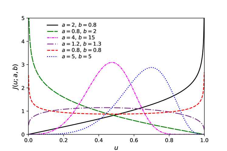
Figure 1: Shapes of the pdf of the Kumaraswamy distribution $J(u;a,b)=abu^{a-1}(1-u^{a})^{b-1},$ for $u\in(0,1)$ and different values of $a$ and $b$.

To demonstrate the advantages of proposed methods over the MTM and MWM approaches, we have included the quantile functions for complete data and various transformations. The sample size for this illustration is $n=50.$ The trimming and winsorizing proportions are 10% (lower) and 20% (upper) for the left panel in Figure 2. The parameters for the $J$ function are indicated in the legend on the right panel in Figure 2.

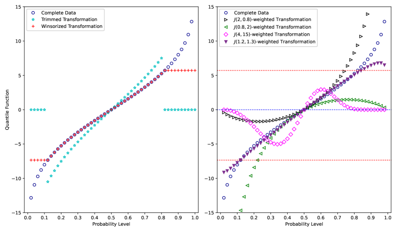
Figure 2: Quantile functions for complete data and various transformations. The sample size is $n=50$. The trimming/winsorizing proportions are 10% (lower) and 20% (upper) for the left panel. The parameters for the $J$ function are indicated in the legend on the right panel.

From Figure 1 and Figure 2 it can be observed that

• When $a$ and $b$ are greater than 1, the density exhibits a bell-shaped behavior. Consequently, if the goal is to assign lower weights to the endpoints and higher weights to the central region, it is advisable to select $a>1$ and $b>1$. For example, see $J(u;a=4,b=15)$ – magenta-colored curve and $J(u;a=5,b=5)$ – blue-colored curve in Figure 1. These weighting mechanisms generate smooth weights, as illustrated in Figure 2 (right panel, $J(4,15)$ labeled curve).

• When $a<1$ and $b\geq 1$, the density is skewed towards $0$, assigning heavier weights to the lower-order statistics and lighter weights to the higher-order statistics. For example, see $J(u;a=0.8,b=2)$ – green-colored curves in Figures 1 and 2 (right panel). In contrast, when $a\geq 1$ and $b<1$, the density is skewed towards $1$, assigning heavier weights to the higher-order statistics and lighter weights to the lower-order statistics. For example, see $J(u;a=2,b=0.8)$ – black-colored curves in Figures 1 and 2 (right panel). This implies that if one intends to assign more weight to lower-order statistics, it is recommended to choose $a<1$ and $b\geq 1$. Conversely, to assign more weight to higher-order statistics, it is advisable to choose $a\geq 1$ and $b<1$.

• Choosing both $a>1$ and $b>1$, but close to 1, slightly mitigates the influence of extreme values by assigning lower weights to tail observations and heavier weights to the main body of the sample data, as illustrated by the $J(1.2,1.3)$-labeled curves in Figures 1 and 2 (right panel).

• Finally, by selecting both $a<1$ and $b<1$, one can assign greater weights to both tails and lighter weights to the middle-order statistics. For example, see $J(u;a=0.8,b=0.8)$ – red-colored curve in Figure 1.

Therefore, by varying the parameters $a$ and $b$, one can tailor the density to emphasize specific regions of the data, such as assigning heavier weights to central values or shifting focus toward one of the tails. This flexibility is particularly advantageous in claim severity modeling, where the underlying distributions often contain outliers, enabling the development of stable and robust predictive models. We will us the Kumaraswamy density to facilitate a novel weighting strategy for robust $L$-estimators, ensuring to achieve the desired level of efficiency and the robustness. Thus, this paper extends the robust $L$-estimation framework to incorporate weights generated by Kumaraswamy densities, addressing limitations of MTM and MWM in three key aspects:

1. Enhanced Flexibility: By leveraging the parameterization of the Kumaraswamy distribution, this approach does not completely disregard the trimmed sample observations, as in MTM, nor does it down-weight extreme values uniformly, as in MWM. Instead, this method smoothly assigns weights across the entire sample order statistics, enabling the allocation of heavier or lighter weights based on the practitioner’s preferences or the specific requirements of the scientific problem or business application.

2. Robustness and Efficiency: The proposed method retains the robustness characteristic of robust $L$-statistics while enhancing efficiency through optimized weighting schemes. This paper offers both theoretical insights and empirical evidence, demonstrating that the proposed robust estimators outperform trimmed and winsorized $L$-estimators as well as MLE, particularly under heavy-tailed and skewed distributions, and when the sample data is contaminated with outliers.

3. Asymptotic Properties: Building on the foundational asymptotic distributional properties of $L$-statistics established by Chernoff et al. (1967), this paper rigorously derives the asymptotic normality of the proposed $L$-estimators. These theoretical advancements provide a robust framework for evaluating the asymptotic relative efficiency (ARE) of the proposed estimators compared to MLE. Through comprehensive theoretical analysis and simulation studies, this work highlights the adaptability of Kumaraswamy-weighted $L$-estimators to various distributional shapes as illustrated in Figure 2. The proposed methodology demonstrates resilience against outliers and achieves significant efficiency improvements over MLE, particularly for datasets containing outliers, emphasizing its practical relevance and effectiveness in estimating robust and stable predictive loss models.

We close this section with the following lemma.

Lemma 1.

Let $X$ be the Kumaraswamy random variable and $g:(0,1)\to\mathbb{R}$ be a non-degenerate continuous function. Define $Y:=g(X)$. Then being a non-degenerate random variable, it immediately follows that $\mathbb{V}ar[Y]>0$.

3 Parametric Severity Models

We now examine the $L$-estimation methodology presented in Section 2 across four parametric examples: the location-scale family, Pareto, lognormal, and Fréchet models. The asymptotic performance of the $L$-estimators is evaluated in terms of asymptotic relative efficiency (ARE) compared to the maximum likelihood estimator (MLE). For a scenario involving $k$ parameters, the ARE is defined as follows (see, e.g., Serfling, 1980, van der Vaart, 1998):

$$ARE(\mathcal{C},MLE)=\left(\dfrac{\det\left(\bm{\Sigma}_{\text{\tiny MLE}}\right)}{\det\left(\bm{\Sigma}_{\text{\tiny$\mathcal{C}$}}\right)}\right)^{1/k},$$ (9)

where $\bm{\Sigma}_{\text{\tiny MLE}}$ and $\bm{\Sigma}_{\text{\tiny$\mathcal{C}$}}$ denote the asymptotic covariance matrices of the MLE and $\mathcal{C}$ estimators, respectively, and $\det$ represents the determinant of a square matrix. The primary rationale for using the MLE as a benchmark lies in its optimal asymptotic performance with respect to variability—granted, of course, that this holds “under certain regularity conditions.” For further details, we refer to Serfling (1980, Section 4.1).

3.1 Location-scale Families

Consider $X_{1},X_{2},\ldots,X_{n}\stackrel{{\scriptstyle iid}}{{\sim}}X$, where $X$ is a location-scale random variable with the CDF

$$F(x) =F_{0}\left(\dfrac{x-\theta}{\sigma}\right),\quad-\infty<x<\infty,$$ (10)

where $-\infty<\theta<\infty$ and $\sigma>0$ are, respectively, the location and scale parameters of $X$, and $F_{0}$ is the standard parameter-free version of $F$, i.e., with $\theta=0$ and $\sigma=1$. The corresponding percentile/quantile function of $X$ is given by

$$F^{-1}(u) =\theta+\sigma F_{0}^{-1}(u).$$ (11)

Since we are estimating two unknown parameters, $\theta$ and $\sigma$, we equate the first two sample $L$-moments with their corresponding population $L$-moments. Further, knowing $-\infty<\theta<\infty$ and $\sigma>0$, we choose

$$h_{1}(x) =x\quad\mbox{and}\quad h_{2}(x)=x^{2}.$$ (12)

From Eq. (2), we note that $H_{j}:=h_{j}\circ F^{-1}$. Then, from Eq. (11) and Eq. (12), we have

$$H_{1}(u)=h_{1}\left(F^{-1}(u)\right)=F^{-1}(u)=\theta+\sigma F_{0}^{-1}(u),$$

$$\implies dH_{1}(u)=\sigma\,dF_{0}^{-1}(u),$$

$$H_{2}(u)=h_{2}\left(F^{-1}(u)\right)=\theta^{2}+2\theta\sigma\,F_{0}^{-1}(u)+\sigma^{2}\left[F_{0}^{-1}(u)\right]^{2},$$

$$\implies dH_{2}(u)=2\theta\sigma\,dF_{0}^{-1}(u)+2\sigma^{2}F_{0}^{-1}(u)\,dF_{0}^{-1}(u).$$

From Eq. (1), the first two sample $L$-moments are given by

$$\begin{cases}\displaystyle\widehat{\mu}_{1}=\dfrac{1}{n}\sum_{i=1}^{n}J\left(\dfrac{i}{n+1}\right)h_{1}(X_{i:n})=\dfrac{1}{n}\sum_{i=1}^{n}J\left(\dfrac{i}{n+1}\right)X_{i:n},\\[15.0pt] \displaystyle\widehat{\mu}_{2}=\dfrac{1}{n}\sum_{i=1}^{n}J\left(\dfrac{i}{n+1}\right)h_{2}(X_{i:n})=\dfrac{1}{n}\sum_{i=1}^{n}J\left(\dfrac{i}{n+1}\right)X_{i:n}^{2}.\end{cases}$$ (13)

The corresponding first two population $L$-moments using Eq. (2) takes the form

$$\begin{cases}\mu_{1}\equiv\mu_{1}\left(\theta,\sigma\right)=\int_{0}^{1}J(u)H_{1}(u)\,du=\int_{0}^{1}J(u)F^{-1}(u)\,du=\theta+\sigma c_{1},\\[10.0pt] \mu_{2}\equiv\mu_{2}\left(\theta,\sigma\right)=\int_{0}^{1}J(u)H_{2}(u)\,du=\int_{0}^{1}J(u)\left[F^{-1}(u)\right]^{2}\,du=\theta^{2}+2\theta\sigma c_{1}+\sigma^{2}c_{2},\end{cases}$$ (14)

where

$$c_{k} \equiv c_{k}\left(F_{0},J\right)=\int_{0}^{1}J(u)\left[F_{0}^{-1}(u)\right]^{k}du,\quad k=1,2.$$ (15)

Since $c_{1}$ and $c_{2}$ do not depend on the parameters to be estimated, equating $\mu_{1}=\widehat{\mu}_{1}$ and $\mu_{2}=\widehat{\mu}_{2}$ yields an explicit system of equations for $\theta$ and $\sigma$ as

$$\left\{\begin{array}[]{lll}\widehat{\theta}_{\mbox{\tiny K}}&=&\widehat{\mu}_{1}-c_{1}\widehat{\sigma}_{\mbox{\tiny K}}=:g_{1}(\widehat{\mu}_{1},\widehat{\mu}_{2}),\\[10.0pt] \widehat{\sigma}_{\mbox{\tiny K}}&=&\sqrt{(\widehat{\mu}_{2}-\widehat{\mu}_{1}^{2})/\eta}=:g_{2}(\widehat{\mu}_{1},\widehat{\mu}_{2}),\quad\text{where}\quad\eta\equiv\eta\left(F_{0},J\right):=c_{2}-c_{1}^{2}.\end{array}\right.$$ (18)

Note 1.

In estimating $\widehat{\sigma}_{\text{\tiny K}}$, it is possible that $\widehat{\mu}_{2}-\widehat{\mu}_{1}^{2}<0$ for certain combinations of an observed sample (small sample size) and the weight-generating function $J$. In such cases, we may need to change the weights-generating function $J$ which will produce $\widehat{\mu}_{2}-\widehat{\mu}_{1}^{2}>0$.

To illustrate this fact, we consider consider a toy sample dataset: $X=(1,2,3,4,5).$ Also consider $a=5=b$. Then it follows that

$$\widehat{\mu}_{1} =\sum_{i=1}^{5}J\left(\dfrac{i}{6}\right)X_{i:5}=4.7398\quad\mbox{and}\quad\widehat{\mu}_{2}=\sum_{i=1}^{5}J\left(\dfrac{i}{6}\right)X_{i:5}^{2}=19.4222,$$

giving us

$$\widehat{\mu}_{2}-\widehat{\mu}_{1}^{2}=-3.0437<0.$$

In this scenario, the estimation formula for $\widehat{\sigma}_{\mbox{\tiny K}}$ as given in Eq. (18) is deemed unsuitable. ∎

From Theorem 1, the entries of the variance-covariance matrix $\Sigma$ evaluated using Eq. (4) are

$$\sigma_{11}^{2} = \int_{0}^{1}\int_{0}^{1}J(v)J(w)K(v,w)\,dH_{1}(v)\,dH_{1}(w)$$

$$= \sigma^{2}\int_{0}^{1}\int_{0}^{1}J(v)J(w)K(v,w)\,dF_{0}^{-1}(v)\,dF_{0}^{-1}(w)$$

$$= \sigma^{2}\Lambda_{1},$$

$$\sigma_{12}^{2} = \int_{0}^{1}\int_{0}^{1}J(v)J(w)K(v,w)\,dH_{1}(v)\,dH_{2}(w)$$

$$= 2\theta\sigma^{2}\int_{0}^{1}\int_{0}^{1}J(v)J(w)K(v,w)\,dF_{0}^{-1}(v)\,dF_{0}^{-1}(w)$$

$$+2\sigma^{3}\int_{0}^{1}\int_{0}^{1}J(v)J(w)K(v,w)\,F_{0}^{-1}(w)\,dF_{0}^{-1}(v)\,dF_{0}^{-1}(w)$$

$$= 2\theta\sigma^{2}\Lambda_{1}+2\sigma^{3}\Lambda_{2},$$

$$\sigma_{22}^{2} = \int_{0}^{1}\int_{0}^{1}J(v)J(w)K(v,w)\,dH_{2}(v)\,dH_{2}(w)$$

$$= 4\theta^{2}\sigma^{2}\int_{0}^{1}\int_{0}^{1}J(v)J(w)K(v,w)\,dF_{0}^{-1}(v)\,dF_{0}^{-1}(w)$$

$$+8\theta\sigma^{3}\int_{0}^{1}\int_{0}^{1}J(v)J(w)K(v,w)\,F_{0}^{-1}(w)\,dF_{0}^{-1}(v)\,dF_{0}^{-1}(w)$$

$$+4\sigma^{4}\int_{0}^{1}\int_{0}^{1}J(v)J(w)K(v,w)\,F_{0}^{-1}(v)\,F_{0}^{-1}(w)\,dF_{0}^{-1}(v)\,dF_{0}^{-1}(w)$$

$$= 4\theta^{2}\sigma^{2}\Lambda_{1}+8\theta\sigma^{3}\Lambda_{2}+4\sigma^{4}\Lambda_{3},$$

where the integral notations

$$\Lambda_{1} \equiv \Lambda_{1}\left(F_{0},J\right)=\int_{0}^{1}\int_{0}^{1}J(v)J(w)K(v,w)\,dF_{0}^{-1}(v)\,dF_{0}^{-1}(w),$$

$$\Lambda_{2} \equiv \Lambda_{2}\left(F_{0},J\right)=\int_{0}^{1}\int_{0}^{1}J(v)J(w)K(v,w)\,F_{0}^{-1}(w)\,dF_{0}^{-1}(v)\,dF_{0}^{-1}(w),$$

$$\Lambda_{3} \equiv \Lambda_{3}\left(F_{0},J\right)=\int_{0}^{1}\int_{0}^{1}J(v)J(w)K(v,w)\,F_{0}^{-1}(v)\,F_{0}^{-1}(w)\,dF_{0}^{-1}(v)\,dF_{0}^{-1}(w),$$

do not depend on the parameters to be estimated.

Corollary 1.

The following inequalities hold:

• $\eta=c_{2}-c_{1}^{2}>0$.

• $\Lambda_{1}\,\Lambda_{3}-\Lambda_{2}^{2}>0.$

Proof.

We use Theorem 3 and Lemma 1 to establish the required inequalities.

• This immediately follows by taking $g(x)=F_{0}^{-1}(x)$ in Lemma 1.

• This follows from Theorem 3 with the following assignments:

  $$f_{1}(x) =\dfrac{J(x)}{f_{0}\left(F_{0}^{-1}(x)\right)}\quad\mbox{and}\quad f_{2}(x)=F_{0}^{-1}(x).\qed$$

Similarly, from Theorem 2, the entries of the matrix $\bm{D}$ are obtained by differentiating the functions $g_{j}$ defined in Eq. (18):

$${\bm{D}} = \left[d_{ij}\right]_{2\times 2}=\left[\left.\frac{\partial g_{i}}{\partial\widehat{\mu}_{j}}\right|_{\widehat{\bm{\mu}}=\bm{\mu}}\right]_{2\times 2}=\dfrac{1}{\sigma\eta}\begin{bmatrix}c_{1}\theta+c_{2}\sigma&-0.5c_{1}\\[5.0pt] -\theta-c_{1}\sigma&0.5\end{bmatrix}.$$ (19)

Therefore, it follows that

$$\left(\widehat{\theta}_{\mbox{\tiny K}},\widehat{\sigma}_{\mbox{\tiny K}}\right) \sim\mathcal{AN}\left(\left(\theta,\sigma\right),\dfrac{1}{n}\bm{S}_{\mbox{\tiny K}}\right),$$ (20)

where

$$\bm{S}_{\mbox{\tiny K}} =\bm{D}\bm{\Sigma}\bm{D}^{\prime}$$

$$=\frac{\sigma^{2}}{\eta^{2}}\begin{bmatrix}\Lambda_{1}c_{2}^{2}-2c_{1}c_{2}\Lambda_{2}+c_{1}^{2}\Lambda_{3}&-\Lambda_{1}c_{1}c_{2}+c_{2}\Lambda_{2}+c_{1}^{2}\Lambda_{2}-c_{1}\Lambda_{3}\\[5.0pt] -\Lambda_{1}c_{1}c_{2}+c_{2}\Lambda_{2}+c_{1}^{2}\Lambda_{2}-c_{1}\Lambda_{3}&\Lambda_{1}c_{1}^{2}-2c_{1}\Lambda_{2}+\Lambda_{3}\end{bmatrix}.$$ (21)

From Eq. (21), it follows that

$$\mbox{det}\left(\bm{S}_{\mbox{\tiny K}}\right) =\dfrac{\sigma^{4}\left(\Lambda_{1}\,\Lambda_{3}-\Lambda_{2}^{2}\right)}{\eta^{2}}.$$ (22)

From Corollary 1, it follows that $\mbox{det}\left(\bm{S}_{\mbox{\tiny K}}\right)>0.$

3.2 Pareto Severity Model

Here we develop the methodology for a single parameter Pareto model. The CDF of the single parameter Pareto random variable $X\sim\mbox{Pareto I}(\alpha,x_{0})$ is given by

$$F(x) =1-\left(\dfrac{x}{x_{0}}\right)^{-\alpha},\quad x>x_{0},$$ (23)

where $\alpha>0$ is the shape parameter and $x_{0}>0$ is assumed to be know. Clearly, from Eq. (23), the corresponding quantile function is

$$F^{-1}(u) =x_{0}(1-u)^{-1/\alpha}.$$ (24)

Since the distribution $F$ contains only one unknown parameter, it is sufficient to use a single $L$-moment for estimation, and we choose $h(x)=\log{(x/x_{0})}$.

With the chosen $h$-function, Eqs. (1) and (2) respectively take the following form

$$\widehat{\mu} = \dfrac{1}{n}\sum_{i=1}^{n}J\left(\dfrac{i}{n+1}\right)\log{(X_{i:n}/x_{0})},$$ (25)

$$\mu = \int_{0}^{1}J(u)H(u)\,du=ab\int_{0}^{1}u^{a-1}\left(1-u^{a}\right)^{b-1}\log{\left(F^{-1}(u)/x_{0}\right)}\,du$$ (26)

$$= -\dfrac{ab}{\alpha}\int_{0}^{1}u^{a-1}\left(1-u^{a}\right)^{b-1}\log{\left(1-u\right)}\,du$$

$$= -\dfrac{I_{1}(a,b)}{\alpha},\quad I_{1}\equiv I_{1}(a,b):=\int_{0}^{1}J(u)\log{\left(1-u\right)}\,du.$$

Note 2.

By using the binomial series expansion for $\left(1-u^{a}\right)^{b-1}$, we can express the population mean $\mu$ from Eq. (26) in terms of hypergeometric function as follows:

$$\mu =\dfrac{b}{\alpha}\sum_{n=0}^{\infty}\dfrac{(-1)^{n}\binom{b-1}{n}}{n+1}\ {}_{2}F_{1}\left(1,a(n+1);a(n+1)+1;1\right).$$ (27)

But for computational purpose, Eq. (26) would be easier by using numerical techniques rather than the form given by Eq. (27). ∎

Now, setting $\mu=\widehat{\mu}$ gives us

$$\widehat{\alpha}_{\mbox{\tiny K}} =-\dfrac{I_{1}(a,b)}{\widehat{\mu}}=:g_{1}\left(\widehat{\mu}\right).$$ (28)

For the asymptotic behavior of $\widehat{\alpha}_{\mbox{\tiny K}}$, the entries of the matrices $\bm{\Sigma}$ and $\bm{D}$, from Theorem 1 and Theorem 2, respectively, for a single dimension are now calculated as:

$$\sigma_{11}^{2} =\int_{0}^{1}\int_{0}^{1}J(v)J(w)K(v,w)\,dH(v)\,dH(w)$$

$$=\dfrac{1}{\alpha^{2}}\int_{0}^{1}\int_{0}^{1}\dfrac{J(v)J(w)K(v,w)}{\overline{v}\,\overline{w}}\,dv\,dw$$

$$=\dfrac{I_{2}(a,b)}{\alpha^{2}}$$

$${\bm{D}} =\left[d_{ij}\right]_{1\times 1}=\left[\left.\frac{\partial g_{1}}{\partial\widehat{\mu}_{1}}\right|_{\widehat{\bm{\mu}}=\bm{\mu}}\right]_{1\times 1}=\dfrac{\alpha^{2}}{I_{1}(a,b)}.$$

Therefore, it follows that

$$\widehat{\alpha}_{\mbox{\tiny K}} \sim\mathcal{AN}\left(\alpha,\dfrac{\alpha^{2}}{n}S_{\mbox{\tiny K}}\right),\quad S_{\mbox{\tiny K}}=\dfrac{I_{2}(a,b)}{I_{1}^{2}(a,b)}.$$ (29)

We note that $\widehat{\alpha}_{\mbox{\tiny MLE}}\sim\mathcal{AN}\left(\alpha,\dfrac{\alpha^{2}}{n}\right).$ Thus, from Eq. (9) and Eq. (29), we have

$$\mbox{ARE}\left(\widehat{\alpha}_{\mbox{\tiny K}},\widehat{\alpha}_{\mbox{\tiny MLE}}\right) =\dfrac{1}{S_{\mbox{\tiny K}}}=\dfrac{I_{1}^{2}(a,b)}{I_{2}(a,b)}.$$ (30)

Table 1: $\mbox{ARE}\left(\widehat{\alpha}_{\mbox{\tiny K}},\widehat{\alpha}_{\mbox{\tiny MLE}}\right)$ for selected values of $a$ and $b$.

$a$	$b$
	0.3	0.5	0.8	1	1.3	2	5	7	15	20
0.3	0.143	0.509	0.973	0.940	0.775	0.459	0.088	0.041	0.006	0.003
0.5	0.140	0.490	0.972	0.975	0.851	0.572	0.170	0.100	0.028	0.016
0.8	0.135	0.464	0.956	0.997	0.920	0.693	0.289	0.201	0.084	0.060
1.0	0.133	0.449	0.941	1.000	0.947	0.750	0.360	0.265	0.129	0.097
1.2	0.130	0.436	0.925	0.998	0.964	0.794	0.422	0.325	0.175	0.138
2.0	0.122	0.392	0.859	0.964	0.982	0.891	0.601	0.509	0.344	0.297
4.0	0.108	0.325	0.728	0.855	0.924	0.928	0.787	0.725	0.596	0.552
5.0	0.103	0.302	0.680	0.808	0.886	0.915	0.820	0.771	0.662	0.623
7.0	0.096	0.268	0.604	0.729	0.818	0.874	0.842	0.812	0.736	0.707
10.0	0.087	0.234	0.524	0.642	0.734	0.809	0.831	0.819	0.778	0.760

We now examine the efficiency of our proposed method of using Kumaraswamy density weights with respect to their MLE estimators using Eq. (9). The numerical values of these AREs, calculated using Eq. (30), are provided in Table 1, with the corresponding interaction plot presented in Figure 3 for various combinations of the parameters $a$ and $b$. From both Table 1 and Figure 3, it is evident that maximum efficiency is achieved when both $a$ and $b$ are close to 1. This weighting mechanism yields lighter tails compared to the observed sample data, effectively controlling the influence of smaller or larger order statistics.

Notably, when $a=1=b$, the $J$-weighted $L$-estimator simplifies to the method of moments (MM). For a single-parameter Pareto distribution, the MM and MLE are identical, resulting in an efficiency of 1.

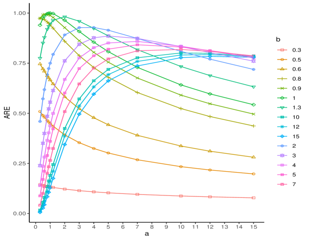
Figure 3: ARE values of the Pareto severity model presented as interactions between the shape parameters $a$ and $b$.

Additionally, the AREs exhibit a threshold-like behavior around $(a=1,b=1)$. Specifically, if a practitioner is willing to tolerate an ARE level of $75\%$ or higher, there are numerous combinations of $a$ and $b$ that provide substantial flexibility in selecting an appropriate weighting mechanism. These combinations facilitate the development of more stable fitted models that remain robust against perturbations in the underlying models. At the same time, they maintain the desired efficiency level and ensure that weights are assigned smoothly—unlike the constant weighting mechanisms employed by MTM and MWM—across the relevant portions of the observed sample data.

3.3 Lognormal Severity Model

Consider $X_{1},X_{2},\ldots,X_{n}\stackrel{{\scriptstyle iid}}{{\sim}}X$, where $X$ has a lognormal distribution function

$$F(x) =\Phi\left(\dfrac{\log{(x-x_{0})}-\theta}{\sigma}\right)\quad x>x_{0},$$ (31)

where $-\infty<\theta<\infty$ and $\sigma>0$ and $\Phi$ is the standard normal cdf. Since $X$ is lognormal, then it is well know that $\log{(X-x_{0})}$ is normal, a member of the location-scale family. So, the results of Section 3.1 are applicable with the two functions:

$$h_{1}(x)=\log{(x-x_{0})}\quad\mbox{and}\quad h_{2}(x)=\left(\log{(x-x_{0})}\right)^{2}.$$

That is, the first two sample $L$-moments corresponding to Eq. (13) are given by

$$\begin{cases}\displaystyle\widehat{\mu}_{1}=\dfrac{1}{n}\sum_{i=1}^{n}J\left(\dfrac{i}{n+1}\right)\log{\left(X_{i:n}-x_{0}\right)},\\[15.0pt] \displaystyle\widehat{\mu}_{2}=\dfrac{1}{n}\sum_{i=1}^{n}J\left(\dfrac{i}{n+1}\right)\left(\log{\left(X_{i:n}-x_{0}\right)}\right)^{2}.\end{cases}$$ (32)

The corresponding first two population $L$-moments are given by Eq. (14) with the developed $H_{1}$ and $H_{2}$ functions. Finally, the estimators $\widehat{\theta}_{\text{\tiny K}}$ and $\widehat{\sigma}_{\text{\tiny K}}$ are solved as in Eq. (18), where the expressions for $\widehat{\mu}_{1}$ and $\widehat{\mu}_{2}$ are found in Eq. (32). From Eq. (20), the asymptotic distribution is given by

$$\left(\widehat{\theta}_{\mbox{\tiny K}},\widehat{\sigma}_{\mbox{\tiny K}}\right) \sim\mathcal{AN}\left(\left(\theta,\sigma\right),\dfrac{1}{n}\bm{S}_{\mbox{\tiny K}}\right),$$ (33)

with $\bm{S}_{\mbox{\tiny K}}$ given by Eq. (21), however, in this case, we use the standard normal distribution $F_{0}(u)=\Phi(u)$ rather than the standardized location-scale distribution employed previously.

From Serfling (2002), we note that the maximum likelihood estimated parameters are given by

$$\left\{\begin{array}[]{lll}\widehat{\theta}_{\mbox{\tiny MLE}}&=&\dfrac{1}{n}\displaystyle\sum_{i=1}^{n}\log{\left(X_{i}-x_{0}\right)},\\[15.0pt] \widehat{\sigma}_{\mbox{\tiny MLE}}&=&\sqrt{\dfrac{1}{n}\displaystyle\sum_{i=1}^{n}\left(\log{(X_{i}-x_{0})}-\widehat{\theta}_{\mbox{\tiny MLE}}\right)^{2}}.\end{array}\right.$$ (36)

Table 2: $\mbox{ARE}\left(\left(\widehat{\theta}_{\mbox{\tiny K}},\widehat{\sigma}_{\mbox{\tiny K}}\right),\left(\widehat{\theta}_{\mbox{\tiny MLE}},\widehat{\sigma}_{\mbox{\tiny MLE}}\right)\right)$ for selected values of $a$ and $b$.

$a$	$b$
	0.3	0.5	0.8	1	1.3	2	5	7	15	20
0.3	0.142	0.264	0.204	0.152	0.103	0.053	0.017	0.014	0.013	0.014
0.5	0.214	0.538	0.582	0.479	0.356	0.203	0.054	0.033	0.012	0.009
0.8	0.176	0.549	0.962	0.950	0.846	0.623	0.262	0.184	0.080	0.058
1.0	0.152	0.479	0.950	1.000	0.955	0.782	0.412	0.314	0.164	0.128
1.2	0.133	0.420	0.892	0.977	0.974	0.853	0.518	0.417	0.247	0.201
2.0	0.092	0.279	0.662	0.782	0.847	0.844	0.672	0.599	0.449	0.401
4.0	0.057	0.155	0.389	0.489	0.565	0.622	0.608	0.584	0.520	0.495
5.0	0.050	0.128	0.323	0.412	0.483	0.544	0.555	0.541	0.499	0.482
7.0	0.040	0.096	0.242	0.314	0.376	0.435	0.467	0.464	0.446	0.437
10.0	0.033	0.071	0.177	0.233	0.283	0.336	0.377	0.380	0.377	0.374

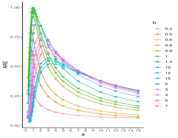
Figure 4: ARE values of the lognormal severity model presented as interactions between the shape parameters $a$ and $b$.

Further, it follows that

$$\left(\widehat{\theta}_{\mbox{\tiny MLE}},\widehat{\sigma}_{\mbox{\tiny MLE}}\right) \sim\mathcal{AN}\left(\left(\theta,\sigma\right),\dfrac{1}{n}\bm{S}_{\mbox{\tiny MLE}}\right),\mbox{ where }\bm{S}_{\mbox{\tiny MLE}}=\sigma^{2}\begin{bmatrix}1&0\\ 0&0.5\end{bmatrix}\mbox{ with }\mbox{det}\left(\bm{S}_{\mbox{\tiny MLE}}\right)=\dfrac{\sigma^{4}}{2}.$$ (37)

Thus, from Eqs. (9), (22), and (37), we have

$$\mbox{ARE}\left(\left(\widehat{\theta}_{\mbox{\tiny K}},\widehat{\sigma}_{\mbox{\tiny K}}\right),\left(\widehat{\theta}_{\mbox{\tiny MLE}},\widehat{\sigma}_{\mbox{\tiny MLE}}\right)\right) =\left(\mbox{det}\left(\bm{S}_{\mbox{\tiny MLE}}\right)/{\mbox{det}\left(\bm{S}_{\mbox{\tiny K}}\right)}\right)^{0.5}=\left(\dfrac{\left(c_{2}-c_{1}^{2}\right)^{2}}{2\left(\Lambda_{1}\Lambda_{3}-\Lambda_{2}^{2}\right)}\right)^{0.5}.$$ (38)

It is important to note that the ARE given by Eq. (38), does not depend on the parameters to be estimated. This is not the case for the payment-per-payment loss variable, as demonstrated by Poudyal (2021) and Poudyal et al. (2024), even for MTM/MWM, where the weights-generating function is much simpler than the one defined in Eq. (7).

The numerical values of these AREs, calculated using Eq. (38), are provided in Table 38, with the corresponding interaction plot presented in Figure 4 for various combinations of the parameters $a$ and $b$. Once again, the maximum efficiency is achieved when both $a$ and $b$ are close to 1. Unlike Figure 3, all ARE values decline sharply for $a>1$, irrespective of the value of $b$. However, for $a>15$, the resulting ARE interaction curves reach a plateau. This behavior occurs because, for larger values of $a$ (regardless of $b$), $J(a,b)$ heavily weights higher-order statistics (right-skewed weighting), making these weighting schemes unsuitable for the lognormal model.

3.4 Fréchet Severity Model

In this subsection we will choose a severity model based on the extreme value distributions. Extreme value distributions are obtained as limiting distributions of greatest (or least) values in random samples of increasing size. Let $X_{1},\cdots,X_{n}$ be iid with distribution function $F$ and let $M_{n}=\max\{X_{1},X_{2},\cdots,X_{n}\}$. Assume that there exit sequence of constants $\{a_{n}>0\}$ and $\{b_{n}\}$ such that $\mathbb{P}\left(a_{n}^{-1}(M_{n}-b_{n})\leq x\right)\rightarrow G(x)$, where $G(x)$ is a non-degenerate cdf. Then according to the Fisher-Tippett-Gnedenko Theorem Fisher and Tippett (1928), the limiting distribution $G(x)$ is the cdf of a Gumbel, a Fréchet or a Weibull distribution. For example, the maximum order statistic from a Pareto distribution converges to a Fréchet distribution as the sample size approaches infinity.

The Fréchet (Fr) distribution (also known as the inverse Weibull distribution) is a special case of the generalized distribution of extreme values. This type II extreme value distribution is used to model maximum values in a dataset, such as flood analysis, maximum rainfall, survival analysis, among others Kotz and Nadarajah (2000). As a member of the location-scale family of distributions, the pdf and cdf are, respectively, given by

$$f(x) = \dfrac{\alpha}{\sigma}\left(\dfrac{x-\theta}{\sigma}\right)^{-(\alpha+1)}\exp\left[-\left(\dfrac{\sigma}{x-\theta}\right)^{\alpha}\right];\quad x>\theta,$$

$$F(x) = \exp\left[-\left(\frac{\sigma}{x-\theta}\right)^{{}^{\alpha}}\right],$$

where $-\infty<\theta<\infty$, $\sigma>0$, and $\alpha>0$ are, respectively, the location, scale, and shape parameters. Since our focus is on estimating financial claim severity models, we set the location parameter $\theta=0$. Thus, we are left to estimate the scale parameter, $\sigma$, and the shape parameter, $\alpha$, of the distribution. The moments and quantile functions are given by

$$\mathbb{E}\left[X^{k}\right] = \sigma^{k}\,\Gamma\left(1-\frac{k}{\alpha}\right);\quad k<\alpha,$$

$$F^{-1}(u) = \sigma\left(-\log(u)\right)^{-1/\alpha}.$$

Like in lognormal model, we take the two functions

$$h_{1}(x) =\log{(x)}\quad\mbox{and}\quad h_{2}(x)=\left(\log{(x)}\right)^{2}.$$ (39)

Thus, with $H_{j}:=h_{j}\circ F^{-1}$, it follows that

$$H_{1}(u)=h_{1}\left(F^{-1}(u)\right)=\log{(\sigma)}-\dfrac{\log{(-\log{(u)})}}{\alpha},$$

$$\implies H_{1}^{{}^{\prime}}(u)=-\dfrac{1}{\alpha u\log{(u)}},$$

$$H_{2}(u)=h_{2}\left(F^{-1}(u)\right)=\left(\log{(\sigma)}\right)^{2}-\dfrac{2\log{(\sigma)}\log{(-\log{(u)})}}{\alpha}+\dfrac{1}{\alpha^{2}}\left(\log{(-\log{(u)})}\right)^{2},$$

$$\implies H_{2}^{{}^{\prime}}(u)=\frac{2\log{(-\log(u))}}{\alpha^{2}u\log(u)}-\frac{2\log(\sigma)}{\alpha u\log(u)}=\frac{2}{\alpha u\log{(u)}}\left(\alpha^{-1}\log{(-\log(u))}-\log{(\sigma)}\right).$$ (41)

Eqs. (1) and (2) respectively take the following form

$$\begin{cases}\widehat{\mu}_{1}=\dfrac{1}{n}\displaystyle\sum_{i=1}^{n}J\left(\dfrac{i}{n+1}\right)\log{(X_{i:n})},\\[15.0pt] \widehat{\mu}_{2}=\dfrac{1}{n}\displaystyle\sum_{i=1}^{n}J\left(\dfrac{i}{n+1}\right)\left(\log{(X_{i:n})}\right)^{2},\end{cases}$$ (42)

$$\begin{cases}\mu_{1}=\int_{0}^{1}J(u)H_{1}(u)\,du=\log{(\sigma)}-\dfrac{1}{\alpha}\kappa_{1},\\[15.0pt] \mu_{2}=\int_{0}^{1}J(u)H_{2}(u)\,du=\left(\log{(\sigma)}\right)^{2}-\dfrac{2\log{(\sigma)}\kappa_{1}}{\alpha}+\dfrac{\kappa_{2}}{\alpha^{2}},\end{cases}$$ (43)

where the two integrals $\kappa_{1}$ and $\kappa_{2}$ are given by

$$\kappa_{1} \equiv\kappa_{1}(J):=\int_{0}^{1}J(u)\log{\left(-\log{(u)}\right)}\,du\mbox{ and }\kappa_{2}\equiv\kappa_{2}(J):=\int_{0}^{1}J(u)\left(\log{\left(-\log{(u)}\right)}\right)^{2}\,du$$ (44)

do not depend on the parameters $\sigma$ and $\alpha$ to be estimated.

Setting $\left(\mu_{1},\mu_{2}\right)=\left(\widehat{\mu}_{1},\widehat{\mu}_{2}\right)$ from Eqs. (42) and (43), and solving for $\sigma$ and $\alpha$, we get the explicit $L$-estimators as

$$\begin{cases}\widehat{\alpha}_{\mbox{\tiny K}}=\sqrt{\dfrac{\tau}{\widehat{\mu}_{2}-\widehat{\mu}_{1}^{2}}}=:g_{1}\left(\widehat{\mu}_{1},\widehat{\mu}_{2}\right),\quad\mbox{where}\quad\tau\equiv\tau(J):=\kappa_{2}-\kappa_{1}^{2},\\[10.0pt] \widehat{\sigma}_{\mbox{\tiny K}}=\exp\left\{\widehat{\mu}_{1}+\dfrac{\kappa_{1}}{\widehat{\alpha}_{\mbox{\tiny K}}}\right\}=:g_{2}\left(\widehat{\mu}_{1},\widehat{\mu}_{2}\right).\end{cases}$$ (45)

Note 3.

Even though the Fréchet distribution is a member of the location-scale family and includes a shape parameter, we do not consider the $h$-functions as defined in Eq. (12), since they do not lead to explicit formulas for the estimated parameters, as shown in Eq. (45), which results from a different choice of $h$-functions from Eq. (39). That is, $F_{0}^{-1}(u)=\left(-\log(u)\right)^{-1/\alpha}$ is not independent of the shape parameter, as $\alpha$ remains present in the expression. ∎

Note 4.

From Corollary 2(i), it follows that the estimated $\widehat{\alpha}_{\mbox{\tiny K}}$ in Eq. (45) is a positive real number (as expected), provided that $\widehat{\mu}_{2}-\widehat{\mu}_{1}^{2}>0,$ which may not hold for certain weights-generating functions $J(\cdot)$, as discussed in Note 1. In such cases, the weights-generating function $J(\cdot)$ must be adjusted to ensure that $\widehat{\mu}_{2}-\widehat{\mu}_{1}^{2}>0.$ ∎

Based on Eqs. (3.4) and (41), the entries for the matrix $\bm{\Sigma}$ from Theorem 1 are given by

$$\sigma_{11}^{2} = \int_{0}^{1}\int_{0}^{1}J(v)J(w)K(v,w)\,dH_{1}(v)\,dH_{1}(w)$$ (46)

$$= \dfrac{1}{\alpha^{2}}\int_{0}^{1}\int_{0}^{1}\dfrac{J(v)J(w)K(v,w)}{vw\log{(v)}\log{(w)}}dv\,dw$$

$$= \dfrac{1}{\alpha^{2}}\Psi_{1}(a,b),$$

$$\sigma_{12}^{2} = \int_{0}^{1}\int_{0}^{1}J(v)J(w)K(v,w)\,dH_{1}(v)\,dH_{2}(w)$$ (47)

$$= \frac{2}{\alpha^{2}}\int_{0}^{1}\int_{0}^{1}\frac{J(v)J(w)K(v,w)}{vw\log{(v)}\log{(w)}}\left(\log{(\sigma)}-\alpha^{-1}\log{(-\log(w))}\right)dv\,dw$$

$$= \frac{2\log{(\sigma)}}{\alpha^{2}}\Psi_{1}(a,b)-\dfrac{2}{\alpha^{3}}\int_{0}^{1}\int_{0}^{1}\frac{J(v)J(w)K(v,w)\log{(-\log(w))}}{vw\log{(v)}\log{(w)}}dv\,dw$$

$$= \frac{2\log{(\sigma)}}{\alpha^{2}}\Psi_{1}(a,b)-\frac{2}{\alpha^{3}}\Psi_{2}(a,b),$$

$$\sigma_{22}^{2} = \int_{0}^{1}\int_{0}^{1}J(v)J(w)K(v,w)\,dH_{2}(v)\,dH_{2}(w)$$ (48)

$$= \dfrac{4}{\alpha^{2}}\int_{0}^{1}\int_{0}^{1}\dfrac{J(v)J(w)K(v,w)}{{vw\log{(v)}\log{(w)}}}\left(\frac{\log{(-\log(v))}}{\alpha}-\log{(\sigma)}\right)\left(\frac{\log{(-\log(w))}}{\alpha}-\log{(\sigma)}\right)dv\,dw$$

$$= \dfrac{4\left(\log{(\sigma)}\right)^{2}}{\alpha^{2}}\int_{0}^{1}\int_{0}^{1}\dfrac{J(v)J(w)K(v,w)}{{vw\log{(v)}\log{(w)}}}dv\,dw$$

$$-\dfrac{4\log{(\sigma)}}{\alpha^{3}}\int_{0}^{1}\int_{0}^{1}\dfrac{J(v)J(w)K(v,w)\log{(-\log(v))}}{{vw\log{(v)}\log{(w)}}}dv\,dw$$

$$-\dfrac{4\log{(\sigma)}}{\alpha^{3}}\int_{0}^{1}\int_{0}^{1}\dfrac{J(v)J(w)K(v,w)\log{(-\log(w))}}{{vw\log{(v)}\log{(w)}}}dv\,dw$$

$$+\dfrac{4}{\alpha^{4}}\int_{0}^{1}\int_{0}^{1}\dfrac{J(v)J(w)K(v,w)\log{(-\log(v))}\log{(-\log(w))}}{{vw\log{(v)}\log{(w)}}}dv\,dw$$

$$= \dfrac{4\left(\log{(\sigma)}\right)^{2}}{\alpha^{2}}\Psi_{1}(a,b)-\dfrac{8\log{(\sigma)}}{\alpha^{3}}\Psi_{2}(a,b)+\dfrac{4}{\alpha^{4}}\Psi_{3},$$

with the obvious double integration notations for $\Psi_{i}\equiv\Psi_{i}(a,b)$ for $i=1,2,3$.

Corollary 2.

For all $a>0$ and $b>0$, the following inequalities hold:

• $\tau=\kappa_{2}-\kappa_{1}^{2}>0.$

• $\Psi_{1}\,\Psi_{2}-\Psi_{2}^{2}>0.$

Proof.

As in Corollary 1, we again use Theorem 3 and Lemma 1 to establish the required inequalities.

• This immediately follows by taking $g(x)=\log{\left(-\log{(x)}\right)}$ in Lemma 1.

• This follows from Theorem 3 with the following assignments:

  $$f_{1}(x) =\dfrac{J(x)}{x\,\log{(x)}}\quad\mbox{and}\quad f_{2}(x)=\log{\left(-\log{(x)}\right)}.\qed$$

The matrix $\bm{D}$ is now calculated as

$${\bm{D}} = \left[d_{ij}\right]_{2\times 2}=\left[\left.\frac{\partial g_{i}}{\partial\widehat{\mu}_{j}}\right|_{\widehat{\bm{\mu}}=\bm{\mu}}\right]_{2\times 2}$$ (49)

$$= \begin{bmatrix}\dfrac{\mu_{1}\sqrt{\tau}}{\left(\mu_{2}-\mu_{1}^{2}\right)^{3/2}}&-\dfrac{\sqrt{\tau}}{2\left(\mu_{2}-\mu_{1}^{2}\right)^{3/2}}\\[20.0pt] \sigma\left(1-\dfrac{\mu_{1}\kappa_{1}}{\sqrt{\tau\left(\mu_{2}-\mu_{1}^{2}\right)}}\right)&\dfrac{\sigma\kappa_{1}}{2\sqrt{\tau\left(\mu_{2}-\mu_{1}^{2}\right)}}\end{bmatrix}$$

$$= \begin{bmatrix}\dfrac{\alpha^{2}\left(\alpha\log{(\sigma)}-\kappa_{1}\right)}{\tau}&-\dfrac{\alpha^{3}}{2\tau}\\[20.0pt] \dfrac{\sigma\left(\kappa_{2}-\alpha\log{(\sigma)}\kappa_{1}\right)}{\tau}&\dfrac{\alpha\sigma\kappa_{1}}{2\tau}\end{bmatrix}.$$

Then, it follows that

$$\left(\widehat{\alpha}_{\mbox{\tiny K}},\widehat{\sigma}_{\mbox{\tiny K}}\right) \sim\mathcal{AN}\left(\left(\theta,\sigma\right),\dfrac{1}{n}\bm{S}_{\mbox{\tiny K}}\right),$$ (50)

where

$$\bm{S}_{\mbox{\tiny K}} =\bm{D}\bm{\Sigma}\bm{D}^{\prime}$$

$$=\dfrac{1}{\tau^{2}}\begin{bmatrix}\alpha^{2}\left(\Psi_{1}\kappa_{1}^{2}-2\Psi_{2}\kappa_{1}+\Psi_{3}\right)&\sigma\left(\Psi_{2}\kappa_{2}-\Psi_{3}\kappa_{1}+\Psi_{2}\kappa_{1}^{2}-\Psi_{1}\kappa_{1}\kappa_{2}\right)\\[5.0pt] \sigma\left(\Psi_{2}\kappa_{2}-\Psi_{3}\kappa_{1}+\Psi_{2}\kappa_{1}^{2}-\Psi_{1}\kappa_{1}\kappa_{2}\right)&\alpha^{-2}\sigma^{2}\left(\Psi_{3}\kappa_{1}^{2}-2\Psi_{2}\kappa_{1}\kappa_{2}+\Psi_{1}\kappa_{2}^{2}\right)\end{bmatrix}.$$ (51)

From Eq. (3.4), it immediately follows that

$$\mbox{det}\left(\bm{S}_{\mbox{\tiny K}}\right) =\dfrac{\sigma^{2}\left(\Psi_{1}\Psi_{3}-\Psi_{2}^{2}\right)}{\tau^{2}}>0,\quad\mbox{from Corollary \ref{cor:IntRelation1}.}$$ (52)

Table 3: $\mbox{ARE}\left(\left(\widehat{\theta}_{\mbox{\tiny K}},\widehat{\sigma}_{\mbox{\tiny K}}\right),\left(\widehat{\theta}_{\mbox{\tiny MLE}},\widehat{\sigma}_{\mbox{\tiny MLE}}\right)\right)$ for selected values of $a$ and $b$.

$a$	$b$
	0.3	0.5	0.8	1	1.3	2	5	7	15	20
0.3	0.041	0.190	0.483	0.472	0.372	0.206	0.073	0.065	0.073	0.083
0.5	0.032	0.163	0.674	0.845	0.824	0.575	0.172	0.108	0.043	0.034
0.8	0.024	0.115	0.536	0.795	0.965	0.953	0.536	0.399	0.191	0.142
1.0	0.021	0.096	0.451	0.691	0.882	0.962	0.681	0.555	0.324	0.260
1.2	0.019	0.083	0.386	0.603	0.794	0.917	0.748	0.643	0.427	0.360
2.0	0.014	0.055	0.244	0.393	0.544	0.696	0.733	0.697	0.586	0.542
4.0	0.009	0.031	0.127	0.207	0.296	0.405	0.508	0.518	0.513	0.505
5.0	0.008	0.026	0.103	0.167	0.241	0.334	0.432	0.447	0.457	0.455
7.0	0.007	0.020	0.074	0.121	0.175	0.246	0.331	0.347	0.368	0.371
10.0	0.005	0.015	0.053	0.085	0.124	0.176	0.244	0.259	0.281	0.287

From Bücher and Segers (2018) we also note that the maximum likelihood estimator of $\sigma$ is given by

$$\widehat{\sigma}_{\mbox{\tiny MLE}} =\left(\dfrac{1}{n}\sum_{i=1}^{n}x_{i}^{-\alpha}\right)^{-1/\alpha_{\mbox{\tiny MLE}}},$$ (53)

where $\alpha_{\mbox{\tiny MLE}}$ is given by the unique zero of the strictly decreasing function

$$\xi(\alpha)=\alpha^{-1}+\sum_{i=1}^{n}x_{i}^{-\alpha}\log{(x_{i})}\left(\sum_{i=1}^{n}x_{i}^{-\alpha}\right)^{-1}-n^{-1}\sum_{i=1}^{n}\log{(x_{i})}.$$

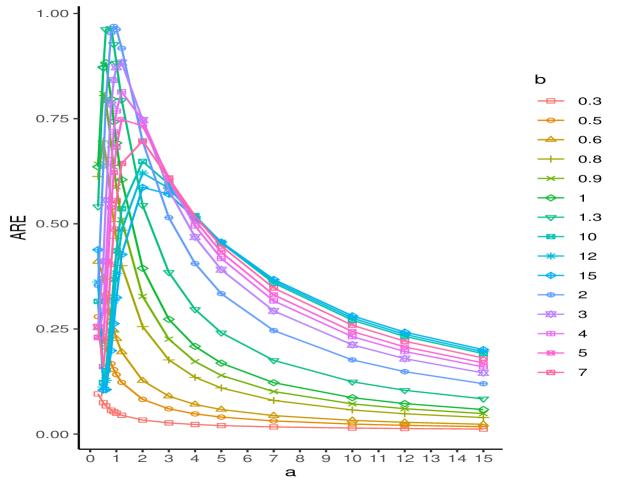
Figure 5: ARE values of the Fréchet severity model presented as interactions between the shape parameters $a$ and $b$.

The asymptotic distribution of the MLE, Bücher and Segers (see, e.g., 2018, Lemma B.3), estimated values is given by

$$\left(\widehat{\alpha}_{\mbox{\tiny MLE}},\widehat{\sigma}_{\mbox{\tiny MLE}}\right) \sim\mathcal{AN}\left(\left(\alpha,\sigma\right),\dfrac{1}{n}\bm{S}_{\mbox{\tiny MLE}}\right),$$ (54)

where

$$\bm{S}_{\mbox{\tiny MLE}} =\dfrac{6}{\pi^{2}}\begin{bmatrix}\alpha^{2}&(\gamma-1)\sigma\\ (\gamma-1)\sigma&(\sigma/\alpha)^{2}\left((\gamma-1)^{2}+\pi^{2}/6\right)\end{bmatrix}\quad\mbox{giving}\quad\mbox{det}\left(\bm{S}_{\mbox{\tiny MLE}}\right)=\dfrac{6\sigma^{2}}{\pi^{2}},$$ (55)

and $\gamma:=-\Gamma^{\prime}(1)=0.57721566490$ is the Euler–Mascheroni constant, Gradshteyn and Ryzhik (2015, p. 914).

Finally, from Eqs. (9), (52), and (55), it follows that

$$\mbox{ARE}\left(\left(\widehat{\theta}_{\mbox{\tiny K}},\widehat{\sigma}_{\mbox{\tiny K}}\right),\left(\widehat{\theta}_{\mbox{\tiny MLE}},\widehat{\sigma}_{\mbox{\tiny MLE}}\right)\right) =\left({\mbox{det}\left(\bm{S}_{\mbox{\tiny MLE}}\right)}/{\mbox{det}\left(\bm{S}_{\mbox{\tiny K}}\right)}\right)^{0.5}=\left(\dfrac{6\pi^{-2}\tau^{2}}{\Psi_{1}\Psi_{3}-\Psi_{2}^{2}}\right)^{0.5},$$ (56)

which, like in Eq. (38), does not depend on the parameters, $\alpha$ and $\sigma$, to be estimated.

The numerical values of these AREs, calculated using Eq. (56), are provided in Table 3, with the corresponding interaction plot presented in Figure 5 for various combinations of the parameters $a$ and $b$. Similar to the Pareto (Table 1) and lognormal (Table 2) cases, the maximum efficiency is achieved when both $a$ and $b$ are close to 1. The interaction curves in Figure 3 and Figure 5 exhibit almost similar patterns: some curves decrease as $a$ increases, while others initially increase and then begin to decrease. In contrast, the interaction curves in Figure 4 all follow the same pattern, first increasing and then decreasing. This behavior may reflect the resemblance of the lognormal density pattern to the normal density, as the logarithmic transformation of lognormal random variables results in a normal distribution. One plausible explanation for the similarity in behavior observed in Figure 3 and Figure 5 is that both Pareto and Fréchet models are characterized by heavy right tails, making them fundamentally distinct from the lognormal distribution, which has a relatively lighter tail.

4 Simulation Study

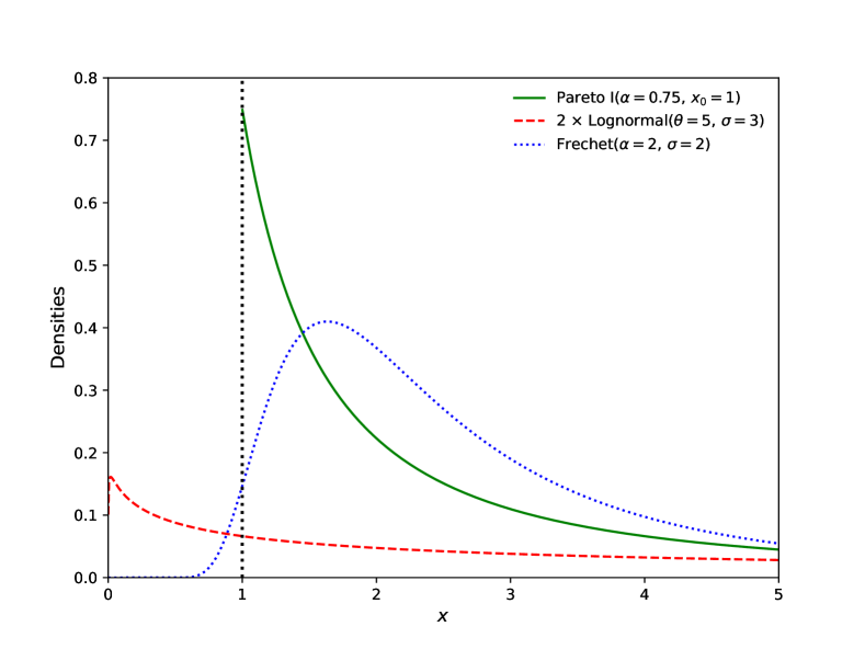
Figure 6: Probability density functions of the three distributions considered in the simulation. For visualization purposes, the pdf of the lognormal distribution is scaled by a factor of 2, as indicated in the legend.

In this section, we extend the theoretical framework presented in Section 3 by conducting simulations to assess key performance metrics of our estimators for Pareto, Lognormal and Fréchet severity models. Probability density functions of the three distributions considered in the simulation study are displayed in Fig. 6. For visualization purposes, the pdf of the lognormal distribution is scaled by a factor of 2, as indicated in the legend.

Specifically, our objectives are to determine the sample size required for estimators to exhibit negligible bias (considering they are asymptotically unbiased), to validate asymptotic normality, and to evaluate finite sample relative efficiencies (REs) as they approach asymptotic relative efficiencies (AREs). For this study, we use the maximum likelihood estimator (MLE) as the baseline for evaluating the relative efficiency of MTM estimators. Therefore, the ARE definition given in Eq. (9) translates to finite sample performance as follows:

$$RE(\mathcal{C},\text{MLE})=\frac{\text{Asymptotic Variance of MLE}}{\text{Small-Sample Variance of $\mathcal{C}$}},$$ (57)

where the numerator corresponds to the asymptotic variance given in Eq. (9), and the denominator represents the small-sample variance of the $L$-estimator, expressed as:

$$\left(\mbox{det}\left\{\left[\mathbb{E}\left[\left(\widehat{\theta}_{i}-\theta_{i}\right)\left(\widehat{\theta}_{j}-\theta_{j}\right)\right]\right]_{i,j=1}^{k}\right\}\right)^{1/2},$$

for a model with $k$ parameters, $\bm{\theta}=\left(\theta_{1},\ldots,\theta_{k}\right)$. The simulation design incorporates the elements as summarized in Table 4.

Table 4: Elements of simulation study.

	Distribution
Element	Pareto I	Lognormal	Fréchet
Parameter(s)	$\alpha=0.75$ and $x_{0}=1$	$\theta=5$ and $\sigma=3$	$\alpha=2$ and $\sigma=2$
Sample Size $(n)$	$100,\,250,\,500,\,750,\,1000$	$100,\,500,\,1000$	$100,\,500,\,1000$
Estimators	MLE and $L$-estimators
$(a,b)$-pairs	$(1,1),\,(.8,.8),\,(.8,2),\,(1.2,1.3),\,(4,15),\,(2,.8),\,\mbox{and}\,(5,5)$

Table 5: Standardized Mean and RE from Pareto I$(\alpha=0.75,x_{0}=1)$. The entries are mean values (with standard errors in parentheses) based on 10,000 samples.

	KS Par		Sample Size
	$a$	$b$	100	250	500	750	1000	$\infty$
Mean = $\widehat{\alpha}/\alpha$	MLE		1.01(.000)	1.00(.000)	1.00(.000)	1.00(.000)	1.00(.000)	1
	1	1	1.01(.000)	1.00(.000)	1.00(.000)	1.00(.000)	1.00(.000)	1
	.8	.8	1.05(.000)	1.00(.000)	1.02(.000)	1.01(.000)	1.01(.000)	1
	.8	2	1.00(.000)	1.03(.000)	1.00(.000)	1.00(.000)	1.00(.000)	1
	1.2	1.3	0.99(.000)	1.00(.000)	1.00(.000)	1.00(.000)	1.00(.000)	1
	4	15	1.00(.010)	1.00(.000)	1.00(.000)	1.00(.000)	1.00(.000)	1
	2	.8	1.07(.000)	1.04(.000)	1.02(.000)	1.02(.000)	1.01(.000)	1
	5	5	0.99(.000)	1.00(.000)	1.00(.000)	1.00(.000)	1.00(.000)	1
RE	MLE		0.94(.060)	0.97(.050)	1.00(.060)	1.00(.040)	1.00(.050)	1
	1	1	0.94(.063)	0.97(.052)	1.00(.061)	1.00(.038)	1.00(.048)	1
	.8	.8	0.70(.048)	0.78(.036)	0.83(.051)	0.84(.033)	0.88(.047)	0.953
	.8	2	0.69(.042)	0.68(.038)	0.69(.033)	0.69(.009)	0.70(.033)	0.693
	1.2	1.3	0.96(.058)	0.95(.054)	0.97(.054)	0.96(.014)	0.98(.048)	0.964
	4	15	0.58(.037)	0.58(.029)	0.59(.030)	0.60(.023)	0.59(.026)	0.596
	2	.8	0.55(.033)	0.64(.029)	0.69(.039)	0.71(.028)	0.75(.039)	0.856
	5	5	0.82(.051)	0.81(.044)	0.82(.039)	0.82(.036)	0.82(.054)	0.820

We have generated $10^{3}$ samples of a specified size $n$ from each chosen distribution $F$ (specifically, the single-parameter Pareto, lognormal, and Fréchet distributions, with their respective densities shown in Figure 6 using Monte Carlo simulations. For each sample, we estimate the parameters of $F$ with MLE and various $L$-estimators and calculate the average mean and RE for these $10^{3}$ estimates. This process is repeated $10$ times, and the $10$ resulting means and REs are averaged again, with their standard deviations also reported. Repeating this procedure allows us to assess the standard errors of the estimated means and REs, providing findings based on a total of $10^{4}$ samples. The reported standardized mean is calculated as the average of $10^{4}$ estimates divided by the true parameter value, with the standard error similarly standardized.

Table 6: Standardized Mean and RE from Lognormal$(\theta=5,\sigma=3))$. The entries are mean values (with standard errors in parentheses) based on 10,000 samples.

	KS Par		$n=100$		$n=500$		$n=1000$		$n\to\infty$
	$a$	$b$	$\widehat{\theta}/\theta$	$\widehat{\sigma}/\sigma$	$\widehat{\theta}/\theta$	$\widehat{\sigma}/\sigma$	$\widehat{\theta}/\theta$	$\widehat{\sigma}/\sigma$	$\widehat{\theta}/\theta$	$\widehat{\sigma}/\sigma$
Mean Values	MLE		1.00(.002)	0.99(.001)	1.00(.001)	1.00(.001)	1.00(.001)	1.00(.000)	1	1
	1	1	1.00(.002)	0.99(.001)	1.00(.001)	1.00(.001)	1.00(.001)	1.00(.000)	1	1
	.8	.8	0.99(.002)	0.97(.001)	1.00(.001)	0.99(.001)	1.00(.001)	0.99(.000)	1	1
	.8	2	1.00(.003)	0.96(.002)	1.00(.001)	0.98(.002)	1.00(.001)	0.99(.001)	1	1
	1.2	1.3	1.01(.002)	1.00(.002)	1.00(.001)	1.00(.001)	1.00(.001)	1.00(.001)	1	1
	4	15	1.00(.003)	0.91(.004)	1.00(.001)	0.98(.002)	1.00(.001)	0.99(.001)	1	1
	2	.8	0.95(.002)	1.01(.003)	0.98(.001)	1.00(.001)	1.00(.001)	1.00(.001)	1	1
	5	5	1.05(.003)	0.88(.004)	1.01(.001)	0.98(.002)	1.00(.001)	0.99(.001)	1	1
Re Values	MLE		1.01(.021)		1.00(.026)		1.00(.029)		1
	1	1	1.01(.021)		1.00(.026)		1.00(.029)		1
	.8	.8	0.95(.021)		0.92(.024)		0.92(.026)		.962
	.8	2	0.69(.019)		0.63(.015)		0.63(.018)		.623
	1.2	1.3	0.95(.020)		0.96(.024)		0.97(.017)		.974
	4	15	0.38(.007)		0.48(.014)		0.51(.017)		.520
	2	.8	0.62(.022)		0.63(.023)		0.64(.022)		.662
	5	5	0.34(.009)		0.49(.010)		0.52(.013)		.555

Table 7: Standardized Mean and RE from Fréchet$(\alpha=2,\sigma=2)$. The entries are mean values (with standard errors in parentheses) based on 10,000 samples.

	KS Par		$n=100$		$n=500$		$n=1000$		$n\to\infty$
	$a$	$b$	$\widehat{\alpha}/\alpha$	$\widehat{\sigma}/\sigma$	$\widehat{\alpha}/\alpha$	$\widehat{\sigma}/\sigma$	$\widehat{\alpha}/\alpha$	$\widehat{\sigma}/\sigma$	$\widehat{\alpha}/\alpha$	$\widehat{\sigma}/\sigma$
Mean Values	MLE		1.01(.002)	1.00(.002)	1.00(.001)	1.00(.001)	1.00(.001)	1.00(.000)	1	1
	1	1	1.02(.002)	1.00(.002)	1.00(.001)	1.00(.001)	1.00(.001)	1.00(.000)	1	1
	.8	.8	1.07(.002)	0.99(.002)	1.03(.002)	1.00(.001)	1.00(.001)	1.00(.000)	1	1
	.8	2	1.01(.002)	1.00(.002)	1.00(.001)	0.98(.001)	1.00(.001)	1.00(.000)	1	1
	1.2	1.3	1.00(.002)	1.01(.002)	1.00(.001)	1.00(.001)	1.00(.001)	1.00(.000)	1	1
	4	15	1.12(.006)	1.02(.002)	1.02(.001)	1.00(.001)	1.01(.001)	1.00(.000)	1	1
	2	.8	1.09(.003)	0.99(.003)	1.04(.003)	1.00(.002)	1.02(.002)	1.00(.001)	1	1
	5	5	1.10(.006)	1.05(.003)	1.02(.002)	1.01(.001)	1.01(.001)	1.00(.001)	1	1
Re Values	MLE		0.93(.041)		0.99(.030)		0.99(.031)		1
	1	1	0.67(.028)		0.68(.020)		0.69(.020)		.691
	.8	.8	0.56(.024)		0.54(.015)		0.54(.015)		.536
	.8	2	0.94(.039)		0.95(.027)		0.94(.025)		.953
	1.2	1.3	0.73(.029)		0.78(.024)		0.78(.021)		.794
	4	15	0.28(.011)		0.45(.011)		0.48(.014)		.513
	2	.8	0.28(.008)		0.26(.007)		0.25(.010)		.244
	5	5	0.24(.007)		0.38(.011)		0.41(.009)		.432

The simulation results are presented in Tables 5, 6, and 7, corresponding to the Pareto I, lognormal, and Fréchet distributions, respectively. The entries of the last column(s) corresponding to $n\to\infty$ in all three tables are included for completeness and are found in Section 3, not from simulations. We see that the MEAN of all Pareto $\alpha$ estimators converges to the parameter $\alpha$ very fast, and the bias practically disappears when $n\geq 500$, except for $J(0.8,0.8)$- and $J(2,0.8)$-weighted $L$-estimators, which are heavily right-weighted and heavy weights assigned at both tails, respectively, as seen in Figure 1. For lognormal and Fréchet models, the convergence of the estimated scale parameter, $\sigma$, is slower than the estimated location parameter, $\theta$. Among all three tables, the maximum relative bias, approximately $-12\%$, is observed for the $J(5,5)$-weighted estimated value of the scale parameter when the sample size is $n=100$.

Similarly, the RE’s converge to their asymptotic counterparts slower in all three tables. Interestingly, for some choices of $a$ and $b$, for example, for $J(0.8,2)$-weighted RE’s for lognormal and for $J(0.8,0.8)$-weighted RE’s for Fréchet models are converging to their corresponding asymptotic counter parts from above.

5 Real Data Analysis

This section assesses the performance of the estimation methods developed in the previous sections by applying them to a real-world dataset. Specifically, we analyze a dataset consisting of 1500 U.S. indemnity losses, which has been extensively studied in the actuarial literature (see, e.g., Frees and Valdez (1998), Poudyal et al. (2024)). Notably, Fung (2024) utilized this dataset to fit Gamma and Inverse-Gaussian models via an intercept-only generalized linear model (GLM) using the score-based weighted likelihood estimation approach, highlighting its suitability for robust modeling. This dataset has been recognized as fitting the lognormal model.

As summarized in Table 8 (top portion), the Kolmogorov-Smirnov (KS) test statistic (see, e.g., Klugman et al., 2019, §15.4.1, p. 360) is computed to be 0.0266. With a significance level of 5%, the corresponding critical value is 0.0351. These results confirm that the lognormal model is a plausible fit for the indemnity loss dataset at the 5% significance level, thereby reinforcing its relevance for this empirical analysis. To further illustrate the benefits of the proposed weighted robust fitting approach, the dataset was slightly modified by replacing its largest observation; 2,173,595, with $10^{7}$ (10 million).

First, we fit the lognormal severity models to the dataset using both MLE and the $J(1.1,1.2)$-weighted $L$-estimators, where the $J(1.1,1.2)$-weighted model assigns slightly lighter weights to both tails of the data compared to the observed sample values, resembling the $J(1.2,1.3)$ curve shown in Figure 2. As presented in Table 8 (top portion), while both MLE and $J(1.1,1.2)$-weighted models produce similar fitted values for $\theta$ and $\sigma$ across both the original and modified datasets, the $J(1.1,1.2)$-weighted model demonstrates greater stability. Specifically, for the original dataset, the $J(1.1,1.2)$-weighted model achieves a $p$-value of $29.02\%$, which is $5.26\%$ higher than the $p$-value of $23.76\%$ obtained from the MLE model.

In contrast, for the modified dataset, the $p$-value of the $J(1.1,1.2)$-weighted model increases relative to the original dataset, while the $p$-value for the MLE model decreases. This indicates the robustness of the $J(1.1,1.2)$-weighted model under data perturbations. Additionally, the KS-test statistic values are consistently lower for the $J(1.1,1.2)$-weighted model compared to the corresponding MLE results, highlighting its superior performance and stability.

Second, purely for illustrative purposes and to enable a clearer visualization, as it is challenging to represent all 1,500 sample observations, a random subsample of size 50 is extracted using seed(123). This subsample is utilized to observe and demonstrate the stability of the proposed $L$-estimation approach. The sampled data are presented below:

1,000	3,436	5,000	7,500	9,000	10,899	14,500	20,000	30,000	95,000
1,500	3,486	5,000	7,525	9,250	11,667	15,000	25,000	30,000	153,874
1,913	4,000	5,010	8,500	9,500	12,100	19,500	25,187	32,000	337,500
2,500	5,000	6,000	8,939	10,000	12,875	20,000	30,000	65,000	412,998
2,500	5,000	6,750	9,000	10,199	14,500	20,000	30,000	74,970	2,173,595

Similar to the approach applied to the original dataset, we modified the sampled dataset to demonstrate the advantages of weighted robust fitting. Specifically, the largest observation, 2,173,595, was replaced with $10^{7}$ (10 million). We then refit the lognormal models to the sampled dataset using MLE and various $J(a,b)$-weighted $L$-estimators, as specified in Table 8 (bottom portion). The resulting fits are visualized in Figure 7—left panel for the sampled dataset and right panel for the modified sampled dataset, respectively. The numerical parameter estimates and goodness-of-fit metrics are presented in Table 8 (bottom portion).

Table 8: MLE and Kumaraswamy weighted estimators of $\theta$ and $\sigma$ with their corresponding one-sample Kolmogorov-Smirnov test statistics.

Estimators	$\widehat{\theta}$	$\widehat{\sigma}$	KS Test			$\widehat{\theta}$	$\widehat{\sigma}$	KS Test
			$h$	$p$-value	$D$			$h$	$p$-value	$D$
$-$	Original Data					Modified Original Data
MLE	9.374	1.638	0	0.2376	0.0266	9.375	1.641	0	0.2303	0.0268
$J(1.1,1.2)$	9.381	1.627	0	0.2902	0.0252	9.382	1.628	0	0.2932	0.0252
$-$	Sampled Data					Modified Sampled Data
MLE	9.536	1.428	0	0.2657	0.1387	9.566	1.547	0	0.1343	0.1609
$J(0.8,2.0)$	9.911	1.970	1	0.0012	0.2671	9.914	1.973	1	0.0012	0.2680
$J(1.1,1.2)$	9.572	0.743	0	0.3622	0.1272	9.595	0.887	0	0.3132	0.1328
$J(2.0,0.8)$	8.386	2.549	1	0.0000	0.3619	8.316	2.768	1	0.0000	0.3749
$J(1.4,14.0)$	9.439	1.151	0	0.8912	0.0788	9.439	1.151	0	0.8912	0.0788

Note: For the KS Test column, $h\in\{0,1\}$ represents the hypothesis test result, where $h=0$ indicates that the assumed model is plausible, and $h=1$ indicates that the model is rejected. $D$ denotes the Kolmogorov-Smirnov test statistic,
and the $p$-value represents the probability of observing a test statistic at least as extreme as $D$ under the null hypothesis.

As shown in Table 8, the $J(1.1,1.2)$- and $J(1.4,14)$-weighted models exhibit significantly higher $p$-values compared to the corresponding MLE-fitted model. Notably, transitioning from the MLE to the $J(1.4,14)$-weighted model results in an increase in the $p$-value from $0.2657$ to $0.8912$, representing a $235.42\%$ rise. Furthermore, when moving from the sampled dataset to the modified sampled dataset, the $p$-value for the MLE-fitted model dropped substantially, nearly halving from $26.57\%$ to $13.43\%$. In contrast, the $p$-values for the $J(1.1,1.2)$- and $J(1.4,14)$-weighted models remained virtually unchanged, further highlighting the robustness and stability of the $J(a,b)$-weighted models, provided the parameters $a$ and $b$ are appropriately selected.

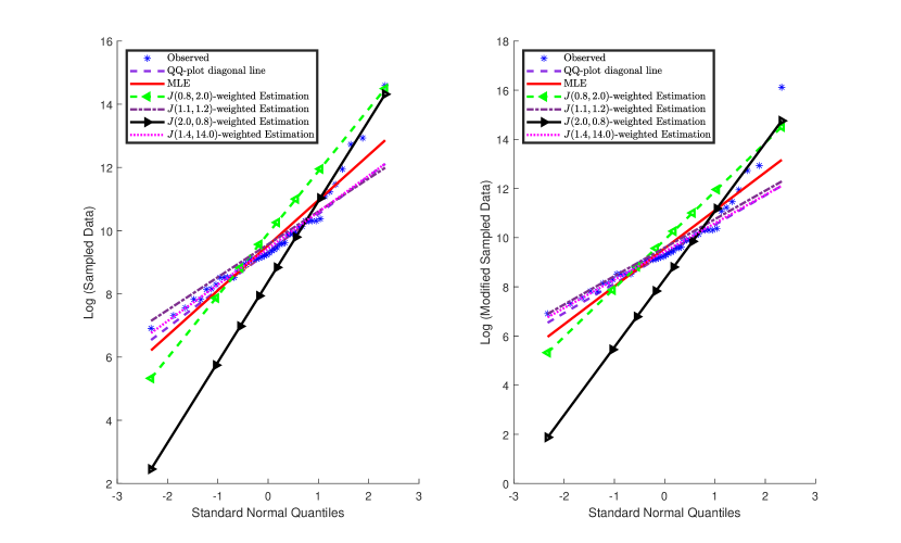
Figure 7: Quantile-quantile plot and lognormal fits for the sampled US Indemnity loss data (left panel) and the modified version of the sampled data (right panel).

Figure 7 offers several insightful observations. Notably, only a few observations (specifically, seven observed stars *) in the right tail deviate from the straight-line pattern, indicating a heavier tail compared to the QQ-plot diagonal line - -. However, the remaining data points closely align with the diagonal line. In the left panel, representing the sampled dataset, the $J(1.1,1.2)$- and $J(1.4,14)$-weighted fits are closely aligned with the QQ-plot diagonal line, providing a more accurate representation of the data points along the diagonal line compared to the MLE.

In contrast, examining the right panel, which corresponds to the modified sampled dataset, the $J(1.1,1.2)$- and $J(1.4,14)$-weighted fits remain robust and unaffected by the data modification, with the data points aligning almost perfectly along the QQ-plot diagonal line. Conversely, the new MLE fit shows significant deviation, particularly in response to the modified largest value of $10^{7}$, highlighting its sensitivity to extreme observations.

The remaining two fits, $J(0.8,2.0)$- and $J(2.0,0.8)$-weighted models, do not perform as well as the MLE fit, as also observed in Figure 4. This is because $J(0.8,2.0)$ assigns disproportionately heavier weights to lower-order statistics (left-skewed weighting), while $J(2.0,0.8)$ heavily weights higher-order statistics (right-skewed weighting), as illustrated in Figures 1 and 2. These weighting schemes are not well-suited for the sampled dataset under consideration.

6 Concluding Remarks

This paper presents a flexible and robust $L$-estimation framework weighted by Kumaraswamy densities, addressing the limitations of the method of trimmed moments (MTM) and the method of winsorized moments (MWM) in modeling claim severity distributions. By incorporating smoothly varying observation-specific weights, the proposed approach effectively balances robustness and efficiency while preserving valuable information from the dataset. Explicit formulations for $L$-estimators were developed for key parametric models, including Pareto, lognormal, and Fréchet distributions, with inferential justification on asymptotic normality and variance-covariance structures. The framework was validated through simulations and a real-world dataset of U.S. indemnity losses, demonstrating superior performance in handling outliers and heavy-tailed distributions for predictive loss severity modeling.

The findings of this study suggest several promising directions for future research. First, while the Kumaraswamy-weighted framework is effective for the models examined, its application to broader classes of claim severity and financial models deserves further exploration, including generalized linear models with similar weighting mechanisms. Second, extending this methodology to multivariate settings could address dependencies often present in actuarial datasets.

Third, insurance losses often exhibit distributional characteristics such as multimodality and outlier contamination. A current trend in the literature involves fitting spliced or mixture loss severity distributions (see, e.g., Blostein and Miljkovic, 2019, Delong et al., 2021, Tomarchio and Punzo, 2020). However, these approaches, typically based on maximum likelihood estimation, may lack stability in cost predictions, particularly under data perturbations or outlier contamination. Investigating the applicability of the weighted $L$-estimation framework for fitting spliced models presents a compelling future direction. Nevertheless, implementing this approach requires the existence of quantile functions, as seen in Eq. (2), and the inferential justification for weighted $L$-estimators in spliced models can be highly challenging, if not infeasible. In such cases, an algorithmic approach, such as simulation-based estimation, could provide an alternative pathway (see, e.g., Efron and Hastie, 2016). Moreover, integrating the framework with machine learning techniques, including ensemble models or neural networks, could offer innovative solutions for predictive modeling in insurance and risk management.

Finally, practical considerations such as computational efficiency and scalability for large datasets remain essential areas for future development. The flexibility and robustness of the proposed framework make it a versatile and promising tool for advancing the precision and stability of actuarial and financial modeling.

References

- Aryal and Zhang (2016) Aryal, G. and Zhang, Q. (2016). Characterizations of Kumaraswamy Laplace distribution with applications. Economic Quality Control, 31(2), 59–70.
- Ash (2000) Ash, R.B. (2000). Probability and Measure Theory. Second edition. Harcourt/Academic Press, Burlington, MA.
- Blostein and Miljkovic (2019) Blostein, M. and Miljkovic, T. (2019). On modeling left-truncated loss data using mixtures of distributions. Insurance: Mathematics & Economics, 85, 35–46.
- Brazauskas et al. (2009) Brazauskas, V., Jones, B.L., and Zitikis, R. (2009). Robust fitting of claim severity distributions and the method of trimmed moments. Journal of Statistical Planning and Inference, 139(6), 2028–2043.
- Bücher and Segers (2018) Bücher, A. and Segers, J. (2018). Maximum likelihood estimation for the Fréchet distribution based on block maxima extracted from a time series. Bernoulli, 24(2), 1427–1462.
- Chernoff et al. (1967) Chernoff, H., Gastwirth, J.L., and Johns, Jr., M. (1967). Asymptotic distribution of linear combinations of functions of order statistics with applications to estimation. Annals of Mathematical Statistics, 38(1), 52–72.
- Cordeiro et al. (2018) Cordeiro, G.M., Machado, E.C., Botter, D.A., and Sandoval, M.C. (2018). The Kumaraswamy normal linear regression model with applications. Communications in Statistics. Simulation and Computation, 47(10), 3062–3082.
- Cordeiro et al. (2010) Cordeiro, G.M., Ortega, E.M.M., and Nadarajah, S. (2010). The Kumaraswamy Weibull distribution with application to failure data. Journal of the Franklin Institute. Engineering and Applied Mathematics, 347(8), 1399–1429.
- Delong et al. (2021) Delong, Ł., Lindholm, M., and Wüthrich, M.V. (2021). Gamma mixture density networks and their application to modelling insurance claim amounts. Insurance: Mathematics & Economics, 101, 240–261.
- Dudley (2002) Dudley, R.M. (2002). Real Analysis and Probability. Cambridge University Press, Cambridge.
- Efron and Hastie (2016) Efron, B. and Hastie, T. (2016). Computer Age Statistical Inference: Algorithms, Evidence, and Data Science. Cambridge University Press, New York.
- Fisher and Tippett (1928) Fisher, R.A. and Tippett, L.H.C. (1928). Limiting forms of the frequency distribution of the largest or smallest member of a sample. Mathematical Proceedings of the Cambridge Philosophical Society, 24(2), 180–190.
- Frees and Valdez (1998) Frees, E.W. and Valdez, E.A. (1998). Understanding relationships using copulas. North American Actuarial Journal, 2(1), 1–25.
- Fung (2022) Fung, T.C. (2022). Maximum weighted likelihood estimator for robust heavy-tail modelling of finite mixture models. Insurance: Mathematics & Economics, 107, 180–198.
- Fung (2024) Fung, T.C. (2024). Robust estimation and diagnostic of generalized linear model for insurance losses: a weighted likelihood approach. Metrika, 00(00), 1–34.
- Gatti and Wüthrich (2024) Gatti, S. and Wüthrich, M.V. (2024). Modeling lower-truncated and right-censored insurance claims with an extension of the MBBEFD class. European Actuarial Journal, 0(0), 1–42.
- Gradshteyn and Ryzhik (2015) Gradshteyn, I.S. and Ryzhik, I.M. (2015). Table of Integrals, Series, and Products. Eighth edition. Elsevier/Academic Press, Amsterdam.
- Hosking (1990) Hosking, J.R.M. (1990). -moments: analysis and estimation of distributions using linear combinations of order statistics. Journal of the Royal Statistical Society. Series B. Methodological, 52(1), 105–124.
- Jones (2009) Jones, M.C. (2009). Kumaraswamy’s distribution: A beta-type distribution with some tractability advantages. Statistical Methodology, 6(1), 70–81.
- Klugman et al. (2019) Klugman, S.A., Panjer, H.H., and Willmot, G.E. (2019). Loss Models: From Data to Decisions. Fifth edition. John Wiley & Sons, Hoboken, NJ.
- Kotz and Nadarajah (2000) Kotz, S. and Nadarajah, S. (2000). Extreme Value Distributions. Imperial College Press, London.
- Kumaraswamy (1980) Kumaraswamy, P. (1980). A generalized probability density function for double-bounded random processe. Journal of Hydrology, 46(1), 79–88.
- Poudyal (2021) Poudyal, C. (2021). Robust estimation of loss models for lognormal insurance payment severity data. ASTIN Bulletin – The Journal of the International Actuarial Association, 51(2), 475–507.
- Poudyal (2024) Poudyal, C. (2024). On the asymptotic normality of trimmed and winsorized L-statistics. Communications in Statistics – Theory and Methods, 0(0), 1–20.
- Poudyal and Brazauskas (2022) Poudyal, C. and Brazauskas, V. (2022). Robust estimation of loss models for truncated and censored severity data. Variance, 15(2), 1–20.
- Poudyal and Brazauskas (2023) Poudyal, C. and Brazauskas, V. (2023). Finite-sample performance of the - and -estimators for the Pareto tail index under data truncation and censoring. J. Stat. Comput. Simul., 93(10), 1601–1621.
- Poudyal et al. (2024) Poudyal, C., Zhao, Q., and Brazauskas, V. (2024). Method of winsorized moments for robust fitting of truncated and censored lognormal distributions. North American Actuarial Journal, 28(1), 236–260.
- Rasmussen and Williams (2006) Rasmussen, C.E. and Williams, C.K.I. (2006). Gaussian Processes for Machine Learning. MIT Press, Cambridge, MA.
- Serfling (1980) Serfling, R. (1980). Approximation Theorems of Mathematical Statistics. John Wiley & Sons, New York.
- Serfling (2002) Serfling, R. (2002). Efficient and robust fitting of lognormal distributions. North American Actuarial Journal, 6(4), 95–109.
- Shreve (2004) Shreve, S.E. (2004). Stochastic Calculus for Finance II: Continuous-time Models. Springer-Verlag, New York.
- Tomarchio and Punzo (2020) Tomarchio, S.D. and Punzo, A. (2020). Dichotomous unimodal compound models: application to the distribution of insurance losses. Journal of Applied Statistics, 47(13-15), 2328–2353.
- Valdora and Yohai (2014) Valdora, M. and Yohai, V.J. (2014). Robust estimators for generalized linear models. Journal of Statistical Planning and Inference, 146, 31–48.
- van der Vaart (1998) van der Vaart, A.W. (1998). Asymptotic Statistics. Cambridge University Press, Cambridge.
- Zhao et al. (2018) Zhao, Q., Brazauskas, V., and Ghorai, J. (2018). Robust and efficient fitting of severity models and the method of Winsorized moments. ASTIN Bulletin – The Journal of the International Actuarial Association, 48(1), 275–309.