Temporal Causal Discovery in Dynamic Bayesian Networks Using Federated Learning

Abstract

Traditionally, learning the structure of a Dynamic Bayesian Network has been centralized, with all data pooled in one location. However, in real-world scenarios, data are often dispersed among multiple parties (e.g., companies, devices) that aim to collaboratively learn a Dynamic Bayesian Network while preserving their data privacy and security. In this study, we introduce a federated learning approach for estimating the structure of a Dynamic Bayesian Network from data distributed horizontally across different parties. We propose a distributed structure learning method that leverages continuous optimization so that only model parameters are exchanged during optimization. Experimental results on synthetic and real datasets reveal that our method outperforms other state-of-the-art techniques, particularly when there are many clients with limited individual sample sizes.

1 Introduction

The learning of Dynamic Bayesian Network (DBN) structures is a crucial technique in causal learning and representation learning. More importantly, it has been applied in various real-world applications, such as modeling gene expression [21], measuring network security [8], studying manufacturing process parameters [47], and recognizing interaction activities [54]. Traditionally, the learning of DBNs has been conducted at a centralized location where all data is aggregated. However, with the rapid advancements in technology and the Internet of Things (IoT) [27] devices, data collection has become significantly more accessible. Consequently, in real-world scenarios, data is typically owned and dispersed among multiple entities, including mobile devices, individuals, companies, and healthcare institutions.

In many cases, these entities, referred to as clients, may lack an adequate number of samples to independently construct a meaningful DBN. They might seek to collaboratively gain comprehensive insights into the DBN structure without disclosing their individual data due to privacy and security concerns. For instance, consider several hospitals aiming to work together to develop a DBN that uncovers the conditional independence relationships among their variables of interest, such as various medical conditions. Sharing patients’ records is clearly prohibited by privacy regulations [2]. Consequently, the sensitive nature of the data renders the centralized aggregation of data from different clients for DBN learning infeasible.

A robust privacy-preserving learning strategy is therefore essential. In recent years, federated learning (FL) [31] has gained significant attention, enabling numerous clients to collaboratively train a machine learning model through a coordinated and privacy-preserving approach. In this framework, each client is not required to share its raw data; instead, they only provide the minimal necessary information, such as model parameters and gradient updates, pertinent to the specific learning task. This approach has been applied across various research domains, including the Internet of Things [20] and recommender systems [7]. Readers may refer to these review papers for more comprehensive insights [23, 51].

Traditionally, score-based learning of DBNs relies on discrete optimization, making it incompatible with common continuous optimization approaches used in federated learning methods. Fortunately, recent work by Zheng et al. [55] and Pamfil et al. [36] have made continuous optimization strategies possible for DBN learning by providing algebraic characterizations of acyclicity. Despite this advancement, directly applying popular federated optimization techniques (FedAvg [31], Ditto [22]) to these continuous formulations remains challenging due to the acyclicity constraint inherent in DBN structure learning.

Contributions.

In this work, we present a federated learning approach for estimating the structure of Dynamic Bayesian Network from observational data (with temporal information) that is horizontally partitioned across different agents. Our contributions are threefold.

• We propose a Federated DBN Learning method 2Dbn based on continuous optimization using the Alternating Direction Method of Multipliers (ADMM). 2Dbn can simultaneously learn contemporaneous and time-lagged causal structure without any implicit assumptions on the underlying graph topology.

• Using extensive simulations and two real-world, high-dimensional datasets, we demonstrate that 2Dbn is scalable and effectively identifies the true underlying DBN graph.

• To our knowledge, this is the first study to explore learning DBN within the FL framework.

Our full code is available on GitHub: https://github.com/PeChen123/2DBN_learning.

Literature Review.

Dynamic Bayesian Network are probabilistic models that extend static Bayesian Networks to represent multi-stage processes by modeling sequences of variables over different stages. Learning DBN involves two key tasks: structure learning (identifying the network topology) and parameter learning (estimating the conditional probabilities). Friedman et al. [12] laid the foundation for this field by developing methods to learn the structure of dynamic probabilistic networks, effectively extending Bayesian Networks to capture temporal dynamics in sequential data. Building on this work, Murphy [32] adapted static Bayesian Network learning techniques for temporal domains, employing methods such as the Expectation-Maximization algorithm for parameter estimation. Advancements in structure learning from time series data were further propelled by Pamfil et al. [36], who developed an extension of Bayesian Network inference using continuous optimization methods. Their approach enabled efficient and scalable learning of DBN structures by formulating the problem as a continuous optimization task with acyclicity constraints tailored for temporal graphs. To address non-linear dependencies in time series data, Tank et al. [48] introduced neural Granger causality methods, which leverage neural networks within the DBN framework to capture complex non-linear interactions. In the field of bioinformatics, Yu et al. [52] enhanced Bayesian Network inference techniques to generate causal networks from observational biological data. Their work demonstrated the practical applicability of DBN in the investigation of intricate biological relationships and regulatory mechanisms. However, traditional DBN learning methods often require centralized data aggregation, which can pose significant privacy risks and scalability challenges, particularly in sensitive domains such as healthcare and genomics. These limitations have spurred interest in privacy-preserving and distributed learning frameworks. Using Federated Learning, DBNs can be trained collaboratively across distributed datasets, enabling secure and scalable model inference while preserving data privacy.

To the best of our knowledge, there is very limited work on federated or privacy-preserving approaches for learning Dynamic Bayesian Networks. However, there are numerous studies based on distributed learning for Bayesian Networks. Gou et al. [16] adopted a two-step procedure that first estimates the BN structures independently using each client’s local dataset and then applies a further conditional independence test. Na and Yang [33] proposed a voting mechanism to select edges that were identified by more than half of the clients. These approaches rely solely on the final graphs that are independently derived from each local dataset, which might result in suboptimal performance due to the limited exchange of information. More importantly, Ng and Zhang [35] proposed a distributed Bayesian learning method based on continuous optimization, using ADMM. Notably, no prior work has tackled distributed learning of DBN.

2 Problem Statement

We consider a scenario with a total of $K$ clients, indexed by $k\in\{1,2,\ldots,K\}$. Each client $k$ possesses its own local dataset consisting of $M$ realizations of a stationary time series. Specifically, for the $k$-th client, we have time series $\{x_{m,t}^{k}\}_{t=0}^{T}$ for $x_{m,t}^{k}\in\mathbb{R}^{d}$, where $m\in\{1,2,\ldots,M\}$ indexes each realization, and $d$ is the number of variables. Due to privacy regulations, these time series cannot be shared directly among clients. For clarity and conciseness, the main text omits the subscript $m$ corresponding to multiple time series, with the complete $m$ notation detailed in the supplementary material §7.1, and consider a generic realization $\{x_{t}^{k}\}_{t=0}^{T}$. In this setting, we assume that the data from all clients follow the same underlying distribution. The extension to non-homogeneous distributions is left for future work (see Sec. 6).

For each client $k$, its dataset (for a single realization) can be written as $\mathcal{D}^{k}=\{x_{t}^{k}\}_{t=p}^{T}$, where $t\in\{p,p+1,\ldots,T\}$ and $p$ denotes the autoregressive order. We model our data using Structural Equation Modeling (SEM) and consider a Vector Autoregressive structure (SVAR) of order $p$:

$$(x_{t}^{k})^{\top}=(x_{t}^{k})^{\top}W+(x_{t-1}^{k})^{\top}A_{1}+\dots+(x_{t-p}^{k})^{\top}A_{p}+(u_{t}^{k})^{\top},$$ (1)

where:

1. $u_{t}^{k}\sim\mathcal{N}(0,I)$ is a vector of centered noise terms, independent across time and variables;

2. $W$ is a weighted adjacency matrix capturing intra-slice dependencies (edges at the same time step);

3. $A_{i}$, for $i\in\{1,\dots,p\}$, are the coefficient matrices capturing inter-slice dependencies (edges across different time steps).

For each client $k$, the effective sample size is $n_{k}=T+1-p$. Given the collection of datasets $X=\bigcup_{k=1}^{K}\mathcal{D}^{k}$ from all clients, the objective is to recover the true $W$ and $A$ in a privacy-preserving manner. We focus on a setup where clients are motivated to collaborate on learning the DBN structure but are only willing to share minimal information, such as model parameters or estimated graphs, about their local datasets. This setup involves horizontal partitioning of the dataset, which means that, while all local datasets share the same set of variables, the sample data differ between clients. The total sample size, $n$, is the sum of the local sample sizes: $n=\sum_{k=1}^{K}n_{k}$.

3 Federated DBN Inference with ADMM

To implement Federated learning to DBN, our method builds on the DYNOTEARS approach introduced by Pamfil et al. [36], which frames the structural learning of linear Dynamical Bayesian Networks as a continuous constrained optimization problem. By incorporating $\ell_{1}$-norm penalties to encourage sparsity, the optimization problem is formulated as follows:

$$\begin{split}\min_{W,A}&\ \ell(W,A)\quad\text{subject to}\quad W\text{ is acyclic},\\ &\ell(W,A)=\frac{1}{2n}\|X_{t}-X_{t}W-X_{(t-p):(t-1)}A\|_{F}^{2}+\lambda_{W}\|W\|_{1}+\lambda_{A}\|A\|_{1}.\end{split}$$ (2)

For the acyclicity constraint, following Zheng et al. [55],

$$h(W)=\mathrm{tr}\left(e^{W\circ W}\right)-d$$

is equal to zero if and only if $W$ is acyclic. Here, $\circ$ represents the Hadamard product (element-wise multiplication) of two matrices. By replacing the acyclicity constraint with the equality constraint $h(W)=0$, the problem can be reformulated as an equality-constrained optimization task.

The ADMM [5] is an optimization algorithm designed to solve convex problems by breaking them into smaller, more manageable subproblems. It is particularly effective for large-scale optimization tasks with complex constraints. By following ADMM framework, we decompose the constrained problem (2) into multiple subproblems and utilize an iterative message-passing approach to converge to the final solution. ADMM proves particularly effective when subproblems have closed-form solutions, which we derive for the first subproblem. To cast problem (2) in an ADMM framework, we reformulate it using local variables $B_{1},\dots,B_{K}\in\mathbb{R}^{d\times d}$ for the intra-slice matrices and $D_{1},\dots,D_{K}\in\mathbb{R}^{d\times d}$ for the inter-slice matrices, along with shared global variables $W\in\mathbb{R}^{d\times d}$ and $A\in\mathbb{R}^{d\times d}$, representing an equivalent formulation:

$$\min_{B_{k},D_{k},W,A}\sum_{k=1}^{K}\ell_{k}(B_{k},D_{k})+\lambda_{W}\|W\|_{1}+\lambda_{A}\|A\|_{1}$$

$$\quad\text{subject to }h(W)=0,$$

$$\quad B_{k}=W,\quad k=1,2,\ldots,K,$$

$$\quad D_{k}=A,\quad k=1,2,\ldots,K.$$

The local variables $B_{1},\dots,B_{K}$ and $D_{1},\dots,D_{K}$ represent the model parameters specific to each client. Notably, this problem resembles the global variable consensus ADMM framework. The constraints $B_{k}=W$ and $D_{k}=A$ are imposed to enforce consistency, ensuring that the local model parameters across clients remain identical.

Since ADMM combines elements of dual decomposition and the augmented Lagrangian method, making it efficient for handling separable objective functions and facilitating parallel computation, we employ the augmented Lagrangian method to transform the constrained problem into a series of unconstrained subproblems. The augmented Lagrangian is given by:

$$\mathcal{L}\left(\{B_{k},D_{k}\}_{k=1}^{K},W,A,\alpha,\{\beta_{k},\gamma_{k}\}_{k=1}^{K};\rho_{1},\rho_{2}\right)=$$

$$\sum_{k=1}^{K}\Bigg{[}\ell_{k}(B_{k},D_{k})+\text{tr}\left(\beta_{k}^{\top}(B_{k}-W)\right)+\frac{\rho_{2}}{2}\|B_{k}-W\|_{F}^{2}$$

$$\quad+\text{tr}\left(\gamma_{k}^{\top}(D_{k}-A)\right)+\frac{\rho_{2}}{2}\|D_{k}-A\|_{F}^{2}\Bigg{]}$$

$$+\lambda_{W}\|W\|_{1}+\lambda_{A}\|A\|_{1}+\alpha h(W)+\frac{\rho_{1}}{2}h(W)^{2},$$

where $\{\beta_{k},\gamma_{k}\}_{k=1}^{K}\in\mathbb{R}^{d\times d}$ and $\alpha\in\mathbb{R}$ are estimations of the Lagrange multipliers; $\rho_{1}$ and $\rho_{2}$ are the penalty coefficients and $\|*\|_{F}$ is Frobenius norm. Then, we have the iterative update rules of ADMM as follows:

Local Updates for $B_{k}$ and $D_{k}$

$$\begin{split}(B_{k}^{(t+1)},D_{k}^{(t+1)})=&\arg\min_{B_{k},D_{k}}\bigg{[}\ell_{k}(B_{k},D_{k})+\text{tr}\left(\beta_{k}^{(t)\top}(B_{k}-W^{(t)})\right)\\ &+\frac{\rho_{2}^{(t)}}{2}\|B_{k}-W^{(t)}\|_{F}^{2}+\text{tr}\left(\gamma_{k}^{(t)\top}(D_{k}-A^{(t)})\right)+\frac{\rho_{2}^{(t)}}{2}\|D_{k}-A^{(t)}\|_{F}^{2}\bigg{]}.\end{split}$$ (3)

Global Updates for $W$ and $A$

$$\begin{split}(W^{(t+1)},A^{(t+1)})=&\arg\min_{W,A}\Bigg{[}\alpha^{(t)}h(W)+\frac{\rho_{1}^{(t)}}{2}h(W)^{2}+\lambda_{W}\|W\|_{1}+\lambda_{A}\|A\|_{1}\\ &+\sum_{k=1}^{K}\left(\text{tr}\left(\beta_{k}^{(t)\top}(B_{k}^{(t+1)}-W)\right)+\frac{\rho_{2}^{(t)}}{2}\|B_{k}^{(t+1)}-W\|_{F}^{2}\right)\\ &+\sum_{k=1}^{K}\left(\text{tr}\left(\gamma_{k}^{(t)\top}(D_{k}^{(t+1)}-A)\right)+\frac{\rho_{2}^{(t)}}{2}\|D_{k}^{(t+1)}-A\|_{F}^{2}\right)\Bigg{]}.\end{split}$$ (4)

Update Dual Variables

$$\begin{split}\beta_{k}^{(t+1)}&=\beta_{k}^{(t)}+\rho_{2}^{(t)}(B_{k}^{(t+1)}-W^{(t+1)}),\\ \gamma_{k}^{(t+1)}&=\gamma_{k}^{(t)}+\rho_{2}^{(t)}(D_{k}^{(t+1)}-A^{(t+1)}),\\ \alpha^{(t+1)}&=\alpha^{(t)}+\rho_{1}^{(t)}h(W^{(t+1)}),\\ \rho_{1}^{(t+1)}&=\phi_{1}\rho_{1}^{(t)},\\ \rho_{2}^{(t+1)}&=\phi_{2}\rho_{2}^{(t)},\end{split}$$ (5)

where $\phi_{1},\phi_{2}\in\mathbb{R}$ are hyperparameters that control how fast the coefficients $\rho_{1},\rho_{2}$ are increased.

As previously mentioned, ADMM is particularly efficient when the optimization subproblems have closed-form solutions. The subproblem in equation (3) is a well-known proximal minimization problem, extensively explored in the field of numerical optimization [9, 37]. For readability, we define the following matrices:

$$S =\frac{1}{n_{k}}X_{t}^{k\top}X_{t}^{k},$$

$$M =\frac{1}{n_{k}}X_{t}^{k\top}X_{(t-p):(t-1)}^{k},$$

$$N =\frac{1}{n_{k}}X_{(t-p):(t-1)}^{k\top}X_{(t-p):(t-1)}^{k},$$

$$P =S+\rho_{2}^{(t)}I,$$

$$Q =N+\rho_{2}^{(t)}I,$$

and vectors:

$$b_{1} =S-\beta_{k}^{(t)}+\rho_{2}^{(t)}W^{(t)},$$

$$b_{2} =M^{\top}-\gamma_{k}^{(t)}+\rho_{2}^{(t)}A^{(t)}.$$

By computing the gradient, we can derive the following closed-form solutions:

• $B_{k}^{(t+1)}$:

  $$\boxed{B_{k}^{(t+1)}=\left(P-MQ^{-1}M^{\top}\right)^{-1}\left(b_{1}-MQ^{-1}b_{2}\right).}$$

• $D_{k}^{(t+1)}$:

  $$\boxed{D_{k}^{(t+1)}=\left(Q-M^{\top}P^{-1}M\right)^{-1}\left(b_{2}-M^{\top}P^{-1}b_{1}\right).}$$

For a comprehensive procedure, we have summarized it in the supplementary material §7.4. The presence of the acyclicity term $h(W)$ prevents us from obtaining a closed-form solution for the problem in equation (4). Instead, the optimization problem can be addressed using first-order methods, such as gradient descent, or second-order methods, like L-BFGS [6]. In this work, we reproduce the approach of Pamfil et al. [36] and employ the L-BFGS method to solve the optimization problem. We have summarized our procedure in Algorithm 1.

Algorithm 1 Distributed DBN Inference with ADMM

0:  Initial parameters $\rho_{1},\rho_{2},\alpha^{(1)},\beta_{1}^{(1)},\ldots,\beta_{K}^{(1)},\gamma_{1}^{(1)},\ldots,\gamma_{K}^{(1)}$; multiplicative factors $\phi_{1},\phi_{2}>1$; initial points $W^{(1)}$ and $A^{(1)}$

1:  for $t=1,2,\ldots$ do

2:     Each client solves problem (3) in parallel

3:     Central server collects $B_{1}^{(t+1)},\ldots,B_{K}^{(t+1)},D_{1}^{(t+1)},\ldots,D_{K}^{(t+1)}$ from all clients

4:     Central server solves problem (4)

5:     Central server sends $W^{(t+1)}$ and $A^{(t+1)}$ to all clients

6:     Central server updates ADMM parameters $\alpha^{(t+1)},\rho_{1}^{(t+1)},\rho_{2}^{(t+1)}$ according to Eq.(5)

7:     Each client updates $\beta_{k}^{(t+1)},\gamma_{k}^{(t+1)}$ according to Eq.(5)

8:  end for

4 Experiments

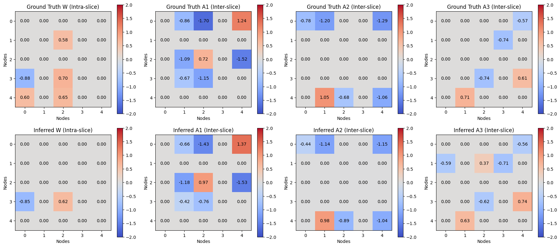
Figure 1: An example result using 2Dbn for Gaussian noise data with $n=500$ samples, $d=5$ variables, an autoregressive order $p=3$, and $K=10$ clients. We set the thresholds $\tau_{w}=\tau_{a}=0.3$. Our algorithm recovers weights close to the ground truth.

In this section, we first study the performance of 2Dbn on simulated data generated by a linear SVAR structure [15]. We then compare it against three linear baseline methods using three evaluation metrics, demonstrating the effectiveness of our proposed method. Figure 1 provides an illustrative example.

Benchmark Methods.

We compare our ADMM-based approach described in Sec. 3, referred to as 2Dbn, with three other methods. The first is a baseline, denoted as Ave, which computes the average of the weighted adjacency matrices estimated by DYNOTEARS [36] from each client’s local dataset, followed by thresholding to determine the edges. The second baseline, referred to as Best, selects the best graph from among those estimated by each client based on the lowest Structural Hamming Distance (SHD) to the ground truth. While this approach is unrealistic in practical scenarios (since it assumes knowledge of the ground truth), it serves as a useful point of reference. For additional context, we also consider DYNOTEARS applied to the combined dataset from all clients, denoted as Alldata. Note that the final graphs produced by Ave may contain cycles, and we do not apply any post-processing steps to remove them, as doing so could reduce performance. Since there is no official source code for DYNOTEARS, we re-implement it using only the numpy and scipy packages in about a hundred lines of code. This simpler, self-contained implementation eases understanding and reusability compared to available versions on GitHub.

Evaluation Metrics.

We use three metrics to evaluate performance: Structural Hamming Distance, True Positive Rate (TPR), and False Discovery Rate (FDR). SHD measures the dissimilarity between the inferred graph and the ground truth, accounting for missing edges, extra edges, and incorrectly oriented edges [49]. Lower SHD indicates closer alignment with the ground truth. TPR (also known as sensitivity or recall) quantifies the proportion of true edges correctly identified, calculated from true positives and false negatives [13]. Higher TPR means the model identifies more true edges. FDR measures the proportion of false positives among all predicted edges, computed as the ratio of false positives to the sum of false positives and true positives [4]. A lower FDR indicates that most detected edges are correct. Together, these metrics provide a comprehensive understanding of the model’s accuracy in graph structure inference.

Data Generation & Settings.

We generate data following the Structural Equation Model described in Eq. (1). This involves four steps: (1). Constructing weighted graphs $G_{W}$ and $G_{A}$; (2). Creating data matrices $X$ and $Y$ aligned with these graphs; (3). Partitioning the data among $K$ clients as $X_{client}$ and $Y_{client}$; (4). Applying all algorithms to $X_{client}$ and $Y_{client}$ (or $X$ and $Y$) and evaluating their performance. For details of steps (1) and (2), see §7.2. We use Gaussian noise with a standard deviation of 1. The intra-slice DAG is an Erdős-Rényi (ER) graph with a mean degree of 4, and the inter-slice DAG is an ER graph with a mean out-degree of 1. Although this results in very sparse graphs at high $d$, they remain connected under our settings [11]. We set the base of the exponential decay of inter-slice weights to $\eta=1.5$.For the hyperparameters $\lambda_{w}$ and $\lambda_{a}$, we generate heatmaps to systematically identify their optimal values. These values are documented in the Supplementary Materials (§7.3). We set $\phi_{1}=1.6$ and $\phi_{2}=1.1$ with initial $\rho_{1}=\rho_{2}=1$, and the initial Lagrange multipliers are zero. For DYNOTEARS (and thus Ave and Best), we follow the authors’ recommended hyperparameters. To avoid confusion, we summarize the data shape used in 2Dbn:

• For 2Dbn, $X$ and $Y$ are of size $K\times n^{\prime}\times d$ and $K\times n^{\prime}\times pd$, respectively, where $K$ is the number of clients, $n^{\prime}$ is the number of samples per client, $d$ is the dimensionality, and $p$ is the autoregressive order.

Experiment Settings. We consider two types of experimental settings. First, we fix the number of clients $K$ and increase the number of variables $d$ while maintaining a consistent total sample size $n$. This allows us to assess how well the methods scale with increasing dimensionality. Second, we fix the total sample size $n\in\{256,512\}$ and vary the number of clients $K$ from 2 to 64. This setting evaluates adaptability and robustness as the data becomes more distributed.

4.1 Varying Number of Variables

In this section, we focus on DBNs with $n=5d$ samples evenly distributed across $K=10$ clients for $d=10,20$, and $n=6d$ for $d\in\{5,15\}$. Note that setting $n=5d$ or $6d$ ensures that each client has an integer number of samples. We generate datasets for each of these cases. Typically, each client has very few samples, making this a challenging scenario.

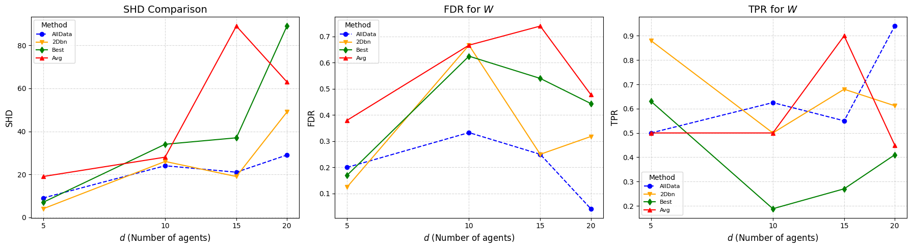
Figure 2: Structure learning results for $W$ in a DBN with Gaussian noise for $d=5,10,15,20$ variables, an autoregressive order $p=1$, and $K=10$ clients.

Figure 2 shows the results for the inferred $W$. The corresponding results for $A$ are provided in §9. Across all tested values of $d$, 2Dbn consistently achieves the lowest SHD compared to Ave and Best, and even outperforms Alldata for $d=5,15$. This advantage may be due to the need for more refined hyperparameter tuning in Alldata. In addition to a lower SHD, 2Dbn achieves a relatively high TPR, close to that of Alldata and higher than that of Best, indicating that 2Dbn accurately identifies most true edges. Moreover, 2Dbn attains a lower FDR than Ave and Best, emphasizing its superior reliability in edge identification under this challenging setup.

4.2 Varying Number of Clients

We now examine scenarios where a fixed total number of samples is distributed among varying numbers of clients. For $d\in\{10,20\}$, we generate $n=512$ samples with $p=1$. These are evenly allocated across $K\in\{2,4,8,16,32,64\}$ clients. For $\lambda_{w}$ and $\lambda_{a}$, we follow the recommendations of [36] for DYNOTEARS, Ave, and Best. For 2Dbn, we select the best regularization parameters from $[0.05,0.5]$ in increments of 0.05 by minimizing SHD.

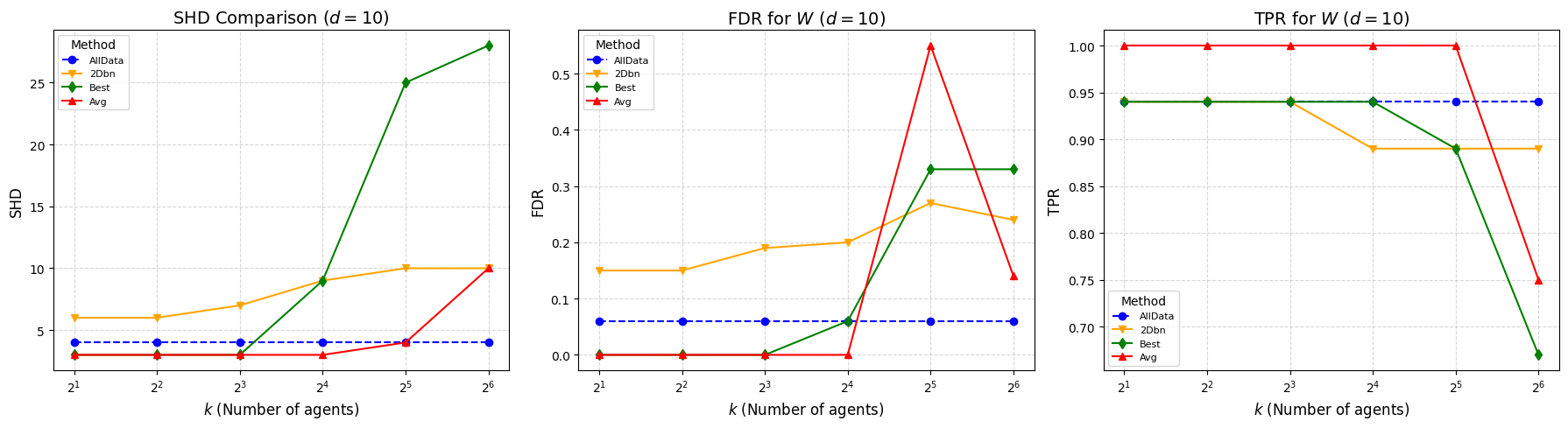
Figure 3: Structure learning for $W$ of a DBN with Gaussian noise for $d=10$ variables, $p=1$, and varying numbers of clients. There are $n=512$ total samples, distributed evenly across $K\in\{2,4,8,16,32,64\}$.

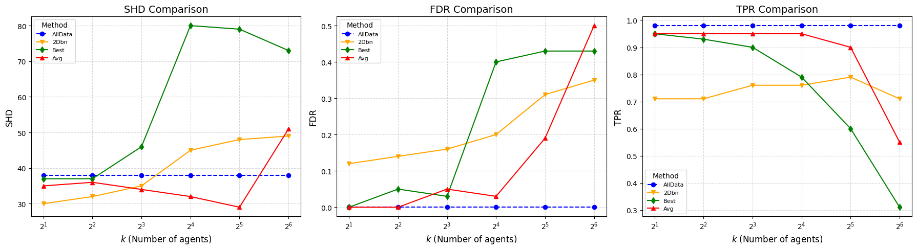
Figure 4: Structure learning for $W$ of a DBN with Gaussian noise for $d=20$ variables, $p=1$, and varying numbers of clients. There are $n=512$ total samples, distributed evenly across $K\in\{2,4,8,16,32,64\}$.

Figures 3 and 4 show the results for $W$ with $d=10$ and $d=20$. The results for $A$ are in §9. As $K$ increases, the TPRs of Ave and Best drop sharply, resulting in high SHDs. Although 2Dbn’s TPR also decreases as $K$ grows, it remains significantly higher than those of the other baselines. For example, with $d=20$ and $K=64$, 2Dbn achieves a TPR of 0.7, while Ave and Best achieve only 0.5 and 0.3, respectively. This highlights the importance of information exchange in the optimization process, enabling 2Dbn to learn a more accurate DBN structure even in highly distributed scenarios.

Next, we consider the case of $n=256$ samples. The corresponding $W$-based results are shown below, and $A$-based results are in §9.

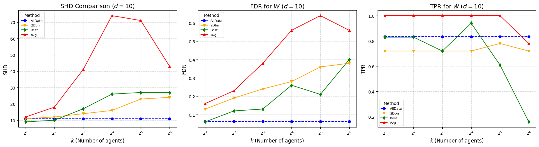
Figure 5: Structure learning for $W$ of a DBN with Gaussian noise for $d=10$ variables, $p=1$, and varying numbers of clients. There are $n=256$ total samples, distributed evenly across $K\in\{2,4,8,16,32,64\}$.

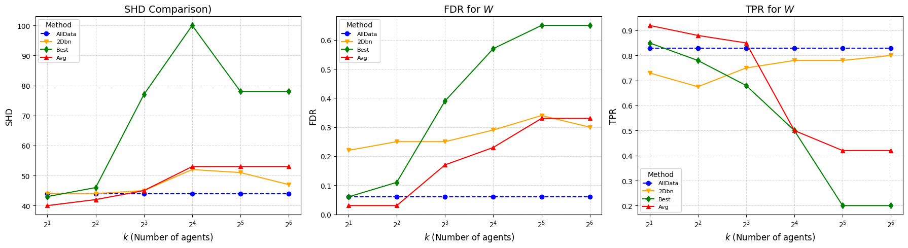
Figure 6: Structure learning for $W$ of a DBN with Gaussian noise for $d=20$ variables, $p=1$, and varying numbers of clients. There are $n=256$ total samples, distributed evenly across $K\in\{2,4,8,16,32,64\}$.

From Figures 5 and 6, 2Dbn consistently attains the lowest SHD compared with Best and Ave. For $d=20$, the TPRs of Ave and Best continue to decline as $K$ increases, whereas 2Dbn’s TPR remains higher for all $K\geq 8$. At extremely high distributions, such as $K=64$ with $d=20$, each client has only 4 samples, leading to non-convergence for Ave and Best. Thus, we compare metrics at $K=32$ for a fair assessment. For $d=10$, while Ave achieves the highest TPR among all methods for all $K$, its FDR is much larger than that of the other methods. This suggests that the thresholding strategy used by Ave may lead to a high number of false positives. Nonetheless, 2Dbn’s TPR for $d=10$ remains close to that of Alldata as $K$ grows.

In some cases, when $K$ or $d$ is small, the other baselines may outperform 2Dbn. For example, with $d=10,n=512$, Ave and Best achieve better SHDs than 2Dbn when $K\leq 16$. This is expected since fewer clients and lower dimensionality provide each client with enough samples for accurate independent structure learning. However, as complexity grows (e.g., $d=20$), 2Dbn outperforms the baselines by maintaining a lower FDR and effectively leveraging distributed information. These findings highlight the importance of both method selection and hyperparameter tuning, as well as potential directions for future research in improving the efficiency of information exchange mechanisms for DBN learning.

5 Applications

5.1 DREAM4

Building on the DREAM4 Challenge [29, 45, 46], our paper focuses on the time-series track of the InSilico_Size100 subchallenge. In this problem, the DREAM4 gene expression data are used to infer gene regulatory networks. The InSilico_Size100 subchallenge dataset contains 5 independent datasets, each consisting of 10 time-series for 100 genes, measured over 21 time steps. We assume that each dataset corresponds to data collected from different hospitals or research centers, thereby motivating our federated approach. More information and data about DREAM4 are available at https://gnw.sourceforge.net/resources/DREAM4%20in%20silico%20challenge.pdf.

Let $X^{g}_{t,r}$ denote the expression level of gene $g$ at time $t\in\{0,1,2,\ldots,20\}$ in replicate $r\in\{0,1,2,\ldots,R\}$. Note that $R$ depends on the dataset used — for instance, if only one dataset is used, then $R=10$. Consequently, $X_{t,r}\in\mathbb{R}^{100}$ and $X_{t}\in\mathbb{R}^{R\times 100}$. In this experiment, we set $p=1$, aligning with the VAR method proposed in the DREAM4 Challenge by Lu et al. [26]. The federated setting of our 2Dbn approach includes $K=5$ clients, each with $R=2$ replicates. Thus, each client contains a time-series dataset for 100 genes over 42 time steps. We found that small regularization parameters, $\lambda_{w}=\lambda_{a}=0.0025$, work well for all DREAM4 datasets. Lu et al. [26] evaluated various methods for learning these networks, including approaches based on Mutual Information(MI), Granger causality, dynamical systems, Decision Trees, Gaussian Processes (GPs), and Dynamic Bayesian Networks. Notably, we did not compare DYNOTEARS in this study, as its source code is not publicly available, and our implemented version did not achieve optimal results. The comparisons were made using AUPR (Area Under the Precision-Recall Curve) and AUROC (Area Under the Receiver Operating Characteristic Curve) across the 5 datasets. From Table. 1, the GP-based method outperforms all others, achieving the highest mean AUPR (0.208) and AUROC (0.728). In terms of AUPR, our 2Dbn approach outperforms the TSNI (ODE-based) method in its non-federated version. Furthermore, the AUPR of 2Dbn is comparable to those of Ebdnet (DBN-based), GCCA (VAR-based), and ARACNE (MI-based) approaches. Importantly, the mean AUROC of 2Dbn surpasses those of GCCA (VAR-based), ARACNE (MI-based), and TSNI (ODE-based) methods, and is close to those of Ebdnet and VBSSMa (DBN-based).

Overall, 2Dbn is comparable to other non-federated benchmarks. However, the GP-based method still achieves superior results in both AUPR and AUROC. One possible reason for this superiority is that the GP-based approach may more effectively capture nonlinear relationships and complex temporal dynamics, which can be challenging in a federated setting where data distributions and conditions vary across sources. Unsurprisingly, the GP-based method outperforms all approaches because Gaussian Processes naturally handle nonlinear dynamics and are more adaptive to varying, complex relationships. In contrast, the 2Dbn model, although suitable for distributed data, might impose stronger parametric assumptions or face computational constraints that limit its ability to capture subtle nonlinear interactions. Thus, we believe GP-based methods could be extended to a distributed approach for structure learning, making them more applicable to real-world problems. We discuss this further in Section 6.

Method	Type	AUPR	AUROC
2Dbn	FED-DBN	0.040	0.600
Ebdnet [41]	DBN	0.043	0.640
VBSSMa [39]	DBN	0.086	0.620
CSId [38]	GP	0.208	0.728
GCCA [39]	VAR	0.050	0.584
TSNI [39]	ODE	0.026	0.566
ARACNE [30]	MI	0.046	0.558

Table 1: Comparison of mean AUPR and mean AUROC scores on the DREAM4 dataset.

5.2 Functional Magnetic Resonance Imaging (FMRI)

In this experiment, we apply the proposed learning methods to estimate connections in the human brain using simulated blood oxygenation level-dependent (BOLD) imaging data [43]. The dataset consists of 28 independent datasets with the number of observed variables $d\in\{5,10,15\}$. Each dataset contains 50 subjects (i.e., 50 ground-truth networks) with 200 time steps. To conduct the experiments, we use simulated time series measurements corresponding to five different human subjects for each $d$ and compute the Average AUROC using the sklearn package.

For the federated setting, we partition the 200 time steps among 5 clients ($K=5$). Detailed information and descriptions of the data are available at https://www.fmrib.ox.ac.uk/datasets/netsim/index.html. In our experiments, we evaluate the proposed method for $d\in\{5,10,15\}$. For $d=5$, we use the 3rd, 6th, 9th, 12th, and 15th subjects from Sim-1.mat. For $d=10$, we use the 2nd, 4th, 6th, 8th, and 10th subjects from Sim-2.mat. Finally, for $d=15$, we use the 1st, 3rd, 5th, 7th, and 9th subjects from Sim-3.mat. Further details of this experiment are provided in the supplementary materials (see §7.5). We compare our method to the economy Statistical Recurrent Units (eSRU) proposed by Khanna and Tan [19] for inferring Granger causality, as well as existing methods based on a Multilayer Perceptron (MLP), a Long Short-Term Memory (LSTM) network [48], and a Convolutional Neural Network (CNN)-based model, the Temporal Causal Discovery Framework (TCDF) [34], on multivariate time series data for $d=15$, as examined by Khanna and Tan [19]. As shown in Tab.2, our proposed 2DBNs achieve an AUROC of 0.74, outperforming the LSTM-based approach and approaching the performance of the CNN-based TCDF method. Even though 2DBNs do not surpass the MLP-based and eSRU-based methods, it is notable that the Federated version of our approach outperforms or closely matches several established non-Federated benchmarks. This outcome is reasonable, as the MLP and eSRU methods rely on deep architectures adept at modeling complex structural dependencies. Notably, our 2DBN method provides a new perspective on this problem by ensuring data security through its Federated approach. This capability is particularly important in scenarios involving sensitive or distributed datasets, as it allows for effective analysis without compromising privacy or data integrity. We have further elaborated on this aspect in Sec.6.

Method	Averaged AUROC
MLP [48]	0.81$\pm$0.04
LSTM [48]	0.70$\pm$0.03
TCDF [34]	0.75$\pm$0.04
eSRU [19]	0.84$\pm$0.03
2DBNs	0.74$\pm$0.04

Table 2: Mean AUROC comparison of different methods for $d=15$.

6 Discussion

We proposed a federated framework for learning DBNs on horizontally partitioned data. Specifically, we designed a distributed DBN learning method using ADMM, where only model parameters are exchanged during optimization. Our experimental results demonstrate that this approach outperforms other state-of-the-art methods, particularly in scenarios with numerous clients, each possessing a small sample size — a common situation in federated learning that motivates client collaboration. Below, we address some limitations of our approach and suggest potential directions for future research.

Assumptions.

We assumed that the structure of the DBN is fixed over time and is identical for all time series in the dataset (i.e., it is the same for all $m\in M$). Relaxing these assumptions could be useful in various ways, such as allowing the structure to change smoothly over time [44]. Another direction for future work is to investigate the behavior of the algorithm on non-stationary or cointegrated time series [28] or in scenarios with confounding variables [17].

Federated Learning.

The proposed ADMM-based approach to federated learning relies on a stateful setup, requiring each participating client to be involved in every round of communication and optimization. This “always-on” requirement can be burdensome in real-world scenarios. For instance, in large-scale deployments, clients such as mobile devices or IoT sensors may experience intermittent connectivity, limited power, or varying levels of availability. Ensuring that all such devices participate consistently and synchronously in every round is often impractical and can result in significant performance bottlenecks. An important future direction is to explore asynchronous techniques, which would enable stateless clients and facilitate cross-device learning. Furthermore, data may be vertically partitioned across clients, meaning that each client owns different variables but collectively aims to perform Bayesian Network Structure Learning (BNSL). Developing a federated approach tailored to this vertical setting represents another promising research direction. Additionally, the ADMM procedure involves sharing model parameters with a central server, raising concerns about potential privacy risks. Research has shown that these parameters can leak sensitive information in certain scenarios, such as with image data [40]. To address this, exploring differential privacy techniques [10] to enhance the protection of shared model parameters is a critical avenue for future work. Moreover, our current work focuses on non-heterogeneous data. However, heterogeneous settings are more applicable to many real-world problems, as clients often differ in computational capabilities, communication bandwidth, and local data distributions. These variations pose significant challenges for model convergence and performance. Several methods have been proposed to address these issues. For example, FedProx [24] incorporates a proximal term to stabilize and unify updates from clients with varying local training conditions, while FedNova [50] normalizes aggregated updates to mitigate the impact of heterogeneous local computational workloads.

Nonlinear Dependencies.

Finally, we emphasize that the linear assumption of our methodology was made purely for simplicity, allowing us to focus on the most salient dynamic and temporal aspects of the problem. It is possible to model more complex nonlinear dependencies using Gaussian Processes [18, 42, 14, 53, 25] or neural networks. Additionally, the least squares loss function can be replaced with logistic loss (or more generally, any exponential family log-likelihood) to model binary data. Further, it would be valuable to consider combinations of continuous and discrete data [3], which are essential for many real-world applications.

7 Supplementary Materials

7.1 Notation of multivariate time-series

After reintroducing the index $m$ for the $M$ realizations, we can stack the data for client $k$. For each client $k$, define $n_{k}=M(T+1-p)$ as the effective sample size. Then, we can write:

$$X_{t}^{k}=X_{t}^{k}W+X_{t-1}^{k}A_{1}+\dots+X_{t-p}^{k}A_{p}+Z^{k},$$

where:

• $X_{t}^{k}$ is a $n_{k}\times d$ matrix whose rows are $(x_{m,t}^{k})^{\top}$ for $m=1,\dots,M$;

• $X_{t-i}^{k}$ are similarly defined time-lagged matrices for $i=1,\dots,p$;

• $Z^{k}$ aggregates the noise terms $(u_{m,t}^{k})^{\top}$.

This formulation allows us to handle multiple realizations per client while maintaining the VAR structure across time and variables. The remaining learning and optmization steps will follow exactly the approach outlined in the main paper.

7.2 Simulation Data Generating:

Intra-slice graph: We use the Erdős-Rényi (ER) model to generate a random, directed acyclic graph (DAG) with a target mean degree $pr$. In the ER model, edges are generated independently using i.i.d. Bernoulli trials with a probability $pr/dr$, where $dr$ is the number of nodes. The resulting graph is first represented as an adjacency matrix and then oriented to ensure acyclicity by imposing a lower triangular structure, producing a valid DAG. Finally, the nodes of the DAG are randomly permuted to remove any trivial ordering, resulting in a randomized and realistic structure suitable for downstream applications.
Inter-slice graph: We still use ER model to generate the weighted matrix. The edges are directed from node $i_{t-1}$ at time $t-1$ to node $j_{t}$ at time $t$. The binary adjacency matrix $A_{\text{bin}}$ is constructed as:

$$A_{i_{t-1},j_{t}}=\begin{cases}1&\text{with probability }pr/dr\quad\text{for edges from node }i_{t-1}\text{ to }j_{t},\\ 0&\text{otherwise}.\end{cases}$$

Assigning Weights: Once the binary adjacency matrix is generated, we assign edge weights from a uniform distribution over the range $[-0.5,-0.3]\cup[0.3,0.5]$ for $W$ and $[-0.5\alpha,-0.3\alpha]\cup[0.3\alpha,0.5\alpha]$ for $A$, where:

$$\alpha=\frac{1}{\eta^{p-1}},$$

and $\eta\geq 1$ is a decay parameter controlling how the influence of edges decreases as time steps get further apart.

7.3 Hyperparameters analysis

In this section, we present the optimal parameter values for each simulation. The following table records the optimal $\lambda_{a}$ and $\lambda_{w}$ values for experiments with varying numbers of variables ($d$). In general, $\lambda_{a}=0.5$ and $\lambda_{w}=0.5$ perform well in all cases. However, when $\lambda_{a},\lambda_{w}>0.5$, the algorithm sometimes outputs zero matrices.

Table 3: Optimal $\lambda_{a}$ and $\lambda_{w}$ values for varying $d$.

	$d=5$	$d=10$	$d=15$	$d=20$
$\lambda_{a}$	0.5	0.5	0.5	0.5
$\lambda_{w}$	0.5	0.5	0.5	0.5

The following tables summarize the optimal $\lambda_{a}$ and $\lambda_{w}$ values for experiments with varying numbers of agents, keeping $n=256$. In general, $\lambda_{a}$ values between 0.4 and 0.5 and $\lambda_{w}$ values between 0 and 0.5 work well. Notably, simulations indicate that the optimal range of $\lambda_{a}$ and $\lambda_{w}$ should be between 0.05 and 0.5, depending on the network topology. Within this range, the error in Structural Hamming Distance (SHD) is typically less than 5 units from the optimal value.

Table 4: Sample Size with 256 and $d=10$

	$k=2$	$k=4$	$k=8$	$k=16$	$k=32$	$k=64$
$\lambda_{a}$	0.05	0.5	0.5	0.4	0.35	0.4
$\lambda_{w}$	0.3	0.5	0.45	0.5	0.25	0.3

Table 5: Sample Size with 256 and $d=20$

	$k=2$	$k=4$	$k=8$	$k=16$	$k=32$	$k=64$
$\lambda_{a}$	0.3	0.2	0.5	0.5	0.5	0.05
$\lambda_{w}$	0.4	0.5	0.5	0.5	0.5	0.25

7.4 Closed form for $B_{k}$ and $D_{k}$

Minimize with respect to $B_{k}$ and $D_{k}$:

$$J(B_{k},D_{k})= \,\ell_{k}(B_{k},D_{k})+\operatorname{Tr}\left(\beta_{k}^{t}(B_{k}-W^{(t)})^{\top}\right)+\frac{\rho_{2}^{t}}{2}\left\|B_{k}-W^{(t)}\right\|_{F}^{2}$$

$$+\operatorname{Tr}\left(\gamma_{k}^{t}(D_{k}-A^{(t)})^{\top}\right)+\frac{\rho_{2}^{t}}{2}\left\|D_{k}-A^{(t)}\right\|_{F}^{2}$$

where:

$$\ell_{k}(B_{k},D_{k})=\frac{1}{2n}\left\|X_{t}-X_{t}B_{k}-X_{(t-p):(t-1)}D_{k}\right\|_{F}^{2}.$$

Due to gradients and optimality conditions, we can set the gradients of $J(B_{k},D_{k})$ with respect to $B_{k}$ and $D_{k}$ to zero. Thus we can have:

Gradient with respect to $B_{k}$:

$$\nabla_{B_{k}}J=-\frac{1}{n}X_{t}^{\top}\left(X_{t}-X_{t}B_{k}-X_{(t-p):(t-1)}D_{k}\right)+\beta_{k}^{t}+\rho_{2}^{t}(B_{k}-W^{(t)})=0.$$

Simplify:

$$(-S+SB_{k}+MD_{k})+\beta_{k}^{t}+\rho_{2}^{t}(B_{k}-W^{(t)})=0$$

$$\implies(S+\rho_{2}^{t}I)B_{k}+MD_{k}=S-\beta_{k}^{t}+\rho_{2}^{t}W^{(t)}$$

$$\implies PB_{k}+MD_{k}=b_{1}.$$

Gradient with respect to $D_{k}$:

$$\nabla_{D_{k}}J=-\frac{1}{n}X_{(t-p):(t-1)}^{\top}\left(X_{t}-X_{t}B_{k}-X_{(t-p):(t-1)}D_{k}\right)+\gamma_{k}^{t}+\rho_{2}^{t}(D_{k}-A^{(t)})=0.$$

Simplify:

$$(-M^{\top}+M^{\top}B_{k}+ND_{k})+\gamma_{k}^{t}+\rho_{2}^{t}(D_{k}-A^{(t)})=0$$

$$\implies M^{\top}B_{k}+(N+\rho_{2}^{t}I)D_{k}=M^{\top}-\gamma_{k}^{t}+\rho_{2}^{t}A^{(t)}$$

$$\implies M^{\top}B_{k}+QD_{k}=b_{2}.$$

7.5 Application in FMRI

In this section, we present the recorded AUROC values for our 2Dbn method, as shown in Table.7.5.

AUROC	1	3	5	7	9
$d=15$	0.68	0.75	0.71	0.77	0.77
$d=10$	0.69	0.77	0.71	0.69	0.83
$d=5$	0.70	0.75	0.76	0.78	0.70

Our model outputs two matrices, $W$ and $A$, which represent strong connections and weak connections, respectively. To produce the final weight matrix, we combine these two matrices using an element-wise sum. We found that $\lambda_{W}=0.05$ and $\lambda_{A}=0.01$ work well across all datasets by several round experiment.

7.6 Application in Dream4

We have attached our AUPR and AUROC for each dataset at Tab.7.6. Similar to the fMRI data, our model outputs two matrices, $W$ and $A$. However, these are interpreted as representing fast-acting and slow-acting influences, respectively. To produce the final weight matrix, we combine these two matrices using an element-wise sum. Based on the hyperparameter analysis by Pamfil et al. [36], we found that $\lambda_{W}=0.0025$ and $\lambda_{A}=0.0025$ work well across all datasets.

Dataset	AUPR	AUROC
1	0.054	0.64
2	0.032	0.58
3	0.041	0.60
4	0.034	0.58
5	0.035	0.62
Mean ± Std	0.040 ± 0.008	0.60 ± 0.022

7.7 Result for $A$

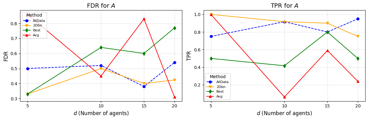
Figure 7: Structure learning results for $A$ in a DBN with Gaussian noise for $d=5,10,15,20$ variables, an autoregressive order $p=1$, and $K=10$ clients.

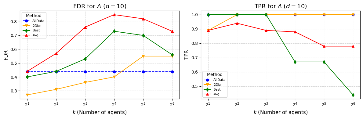
Figure 8: Structure learning for $A$ of DBN with Gaussian noise for $d=10$ variables, $p=1$ Autoregressive order and varying number of clients. There are $n=256$ samples in total, distributed evenly across $K\in\{2,4,8,16,32,64\}$ clients

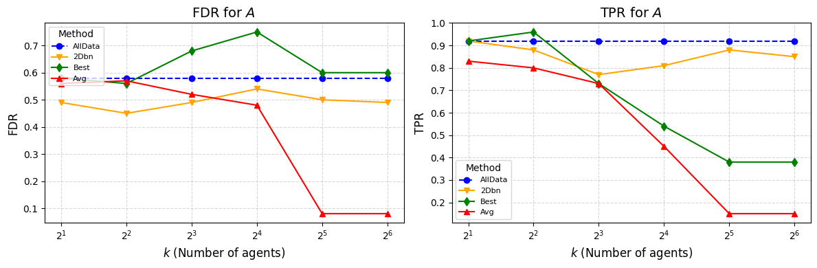
Figure 9: Structure learning for $A$ of DBN with Gaussian noise for $d=20$ variables, $p=1$ Autoregressive order and varying number of clients. There are $n=256$ samples in total, distributed evenly across $K\in\{2,4,8,16,32,64\}$ clients

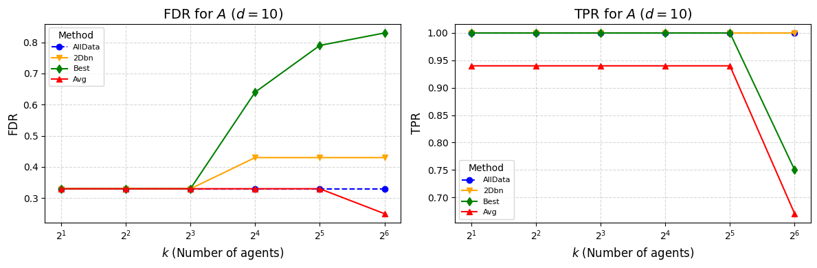
Figure 10: Structure learning for $A$ of DBN with Gaussian noise for $d=10$ variables, $p=1$ Autoregressive order and varying number of clients. There are $n=512$ samples in total, distributed evenly across $K\in\{2,4,8,16,32,64\}$ clients

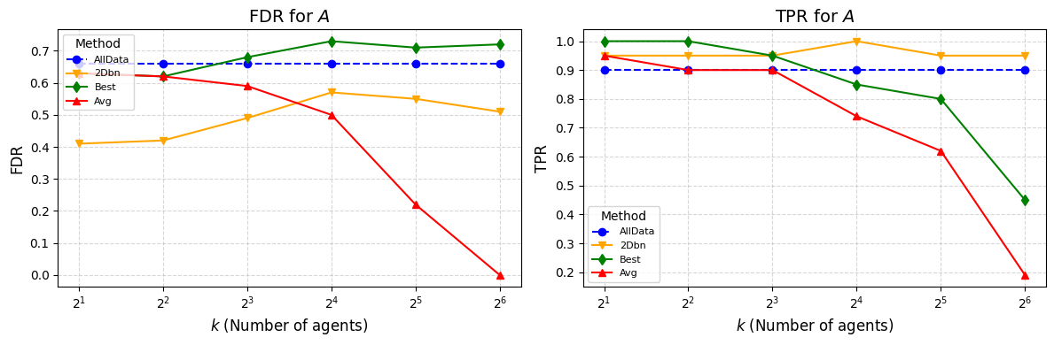
Figure 11: Structure learning for $A$ of DBN with Gaussian noise for $d=20$ variables, $p=1$ Autoregressive order and varying number of clients. There are $n=512$ samples in total, distributed evenly across $K\in\{2,4,8,16,32,64\}$ clients

References

- [1]
- hip [2003] 2003. HIPAA Privacy Rule: Summary of the Privacy Rule. Code of Federal Regulations, 45 CFR Parts 160 and 164. Available at: https://www.hhs.gov/hipaa/for-professionals/privacy/laws-regulations/index.html.
- Andrews et al. [2019] Bryan Andrews, Joseph Ramsey, and Gregory F. Cooper. 2019. Learning High-dimensional Directed Acyclic Graphs with Mixed Data-types. In Proceedings of Machine Learning Research (Proceedings of Machine Learning Research, Vol. 104). PMLR, 4–21. https://proceedings.mlr.press/v104/andrews19a.html
- Benjamini and Hochberg [1995] Yoav Benjamini and Yosef Hochberg. 1995. Controlling the false discovery rate: a practical and powerful approach to multiple testing. Journal of the Royal Statistical Society: Series B (Methodological) 57, 1 (1995), 289–300.
- Boyd et al. [2011] Stephen Boyd, Neal Parikh, Eric Chu, Borja Peleato, and Jonathan Eckstein. 2011. Distributed Optimization and Statistical Learning via the Alternating Direction Method of Multipliers. Foundations and Trends® in Machine Learning 3, 1 (2011), 1–122.
- Byrd et al. [2003] R. H. Byrd, P. Lu, J. Nocedal, and C. Zhu. 2003. A Limited Memory Algorithm for Bound Constrained Optimization. SIAM Journal on Scientific Computing 16 (2003), 1190–1208. https://doi.org/10.1137/0916069
- Chai et al. [2020] D. Chai, L. Wang, K. Chen, and Q. Yang. 2020. Secure Federated Matrix Factorization. IEEE Intelligent Systems 35, 1 (August 2020), 30–38.
- Chockalingam et al. [2017] Sabarathinam Chockalingam, Wolter Pieters, André Teixeira, and P.H.A.J.M. Gelder. 2017. Bayesian Network Models in Cyber Security: A Systematic Review. 105–122. https://doi.org/10.1007/978-3-319-70290-2_7
- Combettes and Pesquet [2011] P. L. Combettes and J.-C. Pesquet. 2011. Proximal Splitting Methods in Signal Processing. In Fixed-Point Algorithms for Inverse Problems in Science and Engineering, H. H. Bauschke, R. S. Burachik, P. L. Combettes, V. Elser, D. R. Luke, and H. Wolkowicz (Eds.). Springer New York, 185–212. https://doi.org/10.1007/978-1-4419-9569-8_10
- Dwork and Roth [2014] Cynthia Dwork and Aaron Roth. 2014. The Algorithmic Foundations of Differential Privacy. Found. Trends Theor. Comput. Sci. 9, 3–4 (Aug. 2014), 211–407. https://doi.org/10.1561/0400000042
- Erdős and Rényi [1960] Paul Erdős and Alfréd Rényi. 1960. On the Evolution of Random Graphs. Publications of the Mathematical Institute of the Hungarian Academy of Sciences 5 (1960), 17–61.
- Friedman et al. [1998] Nir Friedman, Kevin Murphy, and Stuart Russell. 1998. Learning the structure of dynamic probabilistic networks. In Proceedings of the Fourteenth Conference on Uncertainty in Artificial Intelligence (Madison, Wisconsin) (UAI’98). Morgan Kaufmann Publishers Inc., San Francisco, CA, USA, 139–147.
- Glymour et al. [2019] Clark Glymour, Kun Zhang, and Peter Spirtes. 2019. Review of causal discovery methods based on graphical models. Frontiers in Genetics 10 (2019), 524.
- Gnanasambandam et al. [2024] Raghav Gnanasambandam, Bo Shen, Andrew Chung Chee Law, Chaoran Dou, and Zhenyu Kong. 2024. Deep Gaussian process for enhanced Bayesian optimization and its application in additive manufacturing. IISE Transactions (2024), 1–14.
- Gong et al. [2023] Chang Gong, Di Yao, Chuzhe Zhang, Wenbin Li, and Jingping Bi. 2023. Causal Discovery from Temporal Data: An Overview and New Perspectives. Journal of Artificial Intelligence Research 75 (2023), 231–268.
- Gou et al. [2007] Kui Xiang Gou, Gong Xiu Jun, and Zheng Zhao. 2007. Learning Bayesian Network Structure from Distributed Homogeneous Data. In Eighth ACIS International Conference on Software Engineering, Artificial Intelligence, Networking, and Parallel/Distributed Computing (SNPD 2007), Vol. 3. 250–254. https://doi.org/10.1109/SNPD.2007.472
- Huang et al. [2015] Biwei Huang, Kun Zhang, and Bernhard Schölkopf. 2015. Identification of Time-Dependent Causal Model: a gaussian process treatment. In Proceedings of the 24th International Conference on Artificial Intelligence (Buenos Aires, Argentina) (IJCAI’15). AAAI Press, 3561–3568.
- Jin et al. [2019] Xiaoning Jin, Jun Ni, et al. 2019. Physics-based Gaussian process for the health monitoring for a rolling bearing. Acta astronautica 154 (2019), 133–139.
- Khanna and Tan [2019] Saurabh Khanna and Vincent Yan Fu Tan. 2019. Economy Statistical Recurrent Units For Inferring Nonlinear Granger Causality. ArXiv abs/1911.09879 (2019). https://api.semanticscholar.org/CorpusID:208248131
- Kontar et al. [2021] Raed Kontar, Naichen Shi, Xubo Yue, Seokhyun Chung, Eunshin Byon, Mosharaf Chowdhury, Jionghua Jin, Wissam Kontar, Neda Masoud, Maher Nouiehed, Chinedum E. Okwudire, Garvesh Raskutti, Romesh Saigal, Karandeep Singh, and Zhi-Sheng Ye. 2021. The Internet of Federated Things (IoFT). IEEE Access 9 (2021), 156071–156113. https://doi.org/10.1109/ACCESS.2021.3127448
- Lemoine et al. [2021] Guillaume G. Lemoine, Marie-Pier Scott-Boyer, Baptiste Ambroise, et al. 2021. GWENA: gene co-expression networks analysis and extended modules characterization in a single Bioconductor package. BMC Bioinformatics 22 (2021), 267. https://doi.org/10.1186/s12859-021-04179-4
- Li et al. [2021] Tian Li, Shengyuan Hu, Ahmad Beirami, and Virginia Smith. 2021. Ditto: Fair and Robust Federated Learning Through Personalization. In Proceedings of the 38th International Conference on Machine Learning (Proceedings of Machine Learning Research, Vol. 139), Marina Meila and Tong Zhang (Eds.). PMLR, 6357–6368. https://proceedings.mlr.press/v139/li21h.html
- Li et al. [2020a] Tian Li, Ananda K. Sahu, Ameet Talwalkar, and Virginia Smith. 2020a. Federated Learning: Challenges, Methods, and Future Directions. IEEE Signal Processing Magazine 37, 3 (May 2020), 50–60. https://doi.org/10.1109/MSP.2020.2978741
- Li et al. [2020b] Tian Li, Anit Kumar Sahu, Ameet Talwalkar, and Virginia Smith. 2020b. Federated optimization in heterogeneous networks. In Machine Learning and Systems (MLSys).
- Liu and Liu [2024] Xiao Liu and Xinchao Liu. 2024. A Statistical Machine Learning Approach for Adapting Reduced-Order Models using Projected Gaussian Process. arXiv preprint arXiv:2410.14090 (2024).
- Lu et al. [2021] Jing Lu, Bianca Dumitrascu, Ian C. McDowell, Byung-Jun Jo, Andres Barrera, Lichen K. Hong, and et al. 2021. Causal network inference from gene transcriptional time-series response to glucocorticoids. PLoS Computational Biology 17, 1 (2021), e1008223. https://doi.org/10.1371/journal.pcbi.1008223
- Madakam et al. [2015] Somayya Madakam, R Ramaswamy, and Siddharth Tripathi. 2015. Internet of Things (IoT): A Literature Review. Journal of Computer and Communications 3 (04 2015), 164–173. https://doi.org/10.4236/jcc.2015.35021
- Malinsky and Spirtes [2019] Daniel Malinsky and Peter Spirtes. 2019. Learning the Structure of a Nonstationary Vector Autoregression. In Proceedings of the Twenty-Second International Conference on Artificial Intelligence and Statistics (Proceedings of Machine Learning Research, Vol. 89), Kamalika Chaudhuri and Masashi Sugiyama (Eds.). PMLR, 2986–2994. https://proceedings.mlr.press/v89/malinsky19a.html
- Marbach et al. [2009] D. Marbach, T. Schaffter, C. Mattiussi, and D. Floreano. 2009. Generating Realistic In Silico Gene Networks for Performance Assessment of Reverse Engineering Methods. Journal of Computational Biology 16, 2 (2009), 229–239. https://infoscience.epfl.ch/record/128148
- Margolin et al. [2006] Alexander A. Margolin, Ilya Nemenman, Karen Basso, Chris Wiggins, Gustavo Stolovitzky, Riccardo Dalla Favera, and Andrea Califano. 2006. ARACNE: an algorithm for the reconstruction of gene regulatory networks in a mammalian cellular context. BMC Bioinformatics 7 (2006), S7.
- McMahan et al. [2016] H. B. McMahan, Eider Moore, Daniel Ramage, Seth Hampson, and Blaise Agüera y Arcas. 2016. Communication-Efficient Learning of Deep Networks from Decentralized Data. In International Conference on Artificial Intelligence and Statistics. https://api.semanticscholar.org/CorpusID:14955348
- Murphy [2002] Kevin P. Murphy. 2002. Dynamic Bayesian Networks: Representation, Inference and Learning. Ph.D. Thesis. University of California, Berkeley.
- Na and Yang [2010] Yong-chan Na and Jihoon Yang. 2010. Distributed Bayesian network structure learning. In Proceedings of the 2010 IEEE International Symposium on Industrial Electronics (ISIE). IEEE, 1607–1611. https://doi.org/10.1109/ISIE.2010.5636500
- Nauta et al. [2019] Meike Nauta, Doina Bucur, and Christin Seifert. 2019. Causal Discovery with Attention-Based Convolutional Neural Networks. Machine Learning and Knowledge Extraction 1, 1 (2019), 312–340. https://www.mdpi.com/2504-4990/1/1/19
- Ng and Zhang [2022] Ignavier Ng and Kun Zhang. 2022. Towards Federated Bayesian Network Structure Learning with Continuous Optimization. In Proceedings of the 25th International Conference on Artificial Intelligence and Statistics (AISTATS), Vol. 151. PMLR, Valencia, Spain.
- Pamfil et al. [2020] Razvan Pamfil, Stefan Bauer, Bernhard Schölkopf, and Joachim M. Buhmann. 2020. DYNOTEARS: Structure Learning from Time-Series Data. In Proceedings of the 23rd International Conference on Artificial Intelligence and Statistics (AISTATS). PMLR. http://proceedings.mlr.press/v108/pamfil20a.html
- Parikh and Boyd [2014] N. Parikh and S. Boyd. 2014. Proximal Algorithms. Foundations and Trends in Optimization 1, 3 (January 2014), 127–239. https://doi.org/10.1561/2400000003
- Penfold et al. [2015] Christopher A. Penfold, Ahamed Shifaz, Philip E. Brown, Alexander Nicholson, and David L. Wild. 2015. CSI: a nonparametric Bayesian approach to network inference from multiple perturbed time series gene expression data. Statistical Applications in Genetics and Molecular Biology 14, 3 (Jun 2015), 307–310. https://doi.org/10.1515/sagmb-2014-0082
- Penfold and Wild [2011] Christopher A. Penfold and David L. Wild. 2011. How to infer gene networks from expression profiles, revisited. Interface Focus 1 (2011), 857–870.
- Phong et al. [2018] Le Trieu Phong, Yoshinori Aono, Takuya Hayashi, Lihua Wang, and Shiho Moriai. 2018. Privacy-Preserving Deep Learning via Additively Homomorphic Encryption. Trans. Info. For. Sec. 13, 5 (May 2018), 1333–1345.
- Rau et al. [2010] Andrea Rau, Florence Jaffrézic, Jean-Louis Foulley, and Rebecca W. Doerge. 2010. An empirical Bayesian method for estimating biological networks from temporal microarray data. Statistical Applications in Genetics and Molecular Biology 9 (2010), Article 9. https://doi.org/10.2202/1544-6115.1513 Epub 2010 Jan 15.
- Shen et al. [2023] Bo Shen, Raghav Gnanasambandam, Rongxuan Wang, and Zhenyu James Kong. 2023. Multi-task Gaussian process upper confidence bound for hyperparameter tuning and its application for simulation studies of additive manufacturing. IISE Transactions 55, 5 (2023), 496–508.
- Smith et al. [2011] Stephen M Smith, Karla L Miller, Gholamreza Salimi-Khorshidi, Mathew Webster, Christian F Beckmann, Thomas E Nichols, Joseph D Ramsey, and Mark W Woolrich. 2011. Network modelling methods for FMRI. NeuroImage 54, 2 (2011), 875–891. https://doi.org/10.1016/j.neuroimage.2010.08.063
- Song et al. [2009] Le Song, Mladen Kolar, and Eric P. Xing. 2009. Time-varying dynamic Bayesian networks. In Proceedings of the 22nd International Conference on Neural Information Processing Systems (Vancouver, British Columbia, Canada) (NIPS’09). Curran Associates Inc., Red Hook, NY, USA, 1732–1740.
- Stolovitzky et al. [2007] Gustavo Stolovitzky, Don Monroe, and Andrea Califano. 2007. Dialogue on Reverse-Engineering Assessment and Methods: The DREAM of High-Throughput Pathway Inference. Annals of the New York Academy of Sciences 1115 (2007), 11–22.
- Stolovitzky et al. [2009] Gustavo Stolovitzky, Robert J Prill, and Andrea Califano. 2009. Lessons from the DREAM2 Challenges. Annals of the New York Academy of Sciences 1158 (2009), 159–195.
- Sun et al. [2020] Yanning Sun, Wei Qin, and Zilong Zhuang. 2020. Quality consistency analysis for complex assembly process based on Bayesian networks. Procedia Manufacturing 51 (2020), 577–583. https://doi.org/10.1016/j.promfg.2020.10.081 30th International Conference on Flexible Automation and Intelligent Manufacturing (FAIM2021).
- Tank et al. [2022] A. Tank, I. Covert, N. Foti, A. Shojaie, and E. B. Fox. 2022. Neural Granger Causality. IEEE Transactions on Pattern Analysis and Machine Intelligence 44, 8 (2022), 4267–4279. https://doi.org/10.1109/TPAMI.2021.3065601
- Tsamardinos et al. [2006] Ioannis Tsamardinos, Laura E Brown, and Constantin F Aliferis. 2006. The max-min hill-climbing Bayesian network structure learning algorithm. Machine learning 65, 1 (2006), 31–78.
- Wang et al. [2020] Jianyu Wang, Zachary Charles, Brendan Childers, Yu-Xiang Sun, Suhas Sreehari, Sebastian U Stich, Mikhail Dmitriev, Ameet Talwalkar, and Michael I Jordan. 2020. Federated learning with normalized averaging. In Neural Information Processing Systems (NeurIPS).
- Yang et al. [2019] Qiang Yang, Yang Liu, Tian Chen, and Yongxin Tong. 2019. Federated Machine Learning: Concept and Applications. ACM Transactions on Intelligent Systems and Technology (TIST) 10, 2 (January 2019), 1–19. https://doi.org/10.1145/3308558
- Yu et al. [2004] Jing Yu, V. Anne Smith, Paul P. Wang, Alexander J. Hartemink, and Erich D. Jarvis. 2004. Advances to Bayesian Network Inference for Generating Causal Networks from Observational Biological Data. Bioinformatics 20, 18 (2004), 3594–3603. https://doi.org/10.1093/bioinformatics/bth448
- Yue and Kontar [2024] Xubo Yue and Raed Kontar. 2024. Federated Gaussian Process: Convergence, Automatic Personalization and Multi-fidelity Modeling. IEEE Transactions on Pattern Analysis and Machine Intelligence (2024).
- Zeng et al. [2016] Zhiya Zeng, Xia Jiang, and Richard Neapolitan. 2016. Discovering causal interactions using Bayesian network scoring and information gain. BMC Bioinformatics 17 (2016), 221. https://doi.org/10.1186/s12859-016-1084-8
- Zheng et al. [2018] Xun Zheng, Bryon Aragam, Pradeep K. Ravikumar, and Eric P. Xing. 2018. DAGs with NO TEARS: Continuous optimization for structure learning. In Advances in Neural Information Processing Systems 31. Curran Associates, Inc., 9472–9483.