Universal Inceptive GNNs by Eliminating the Smoothness-generalization Dilemma

Abstract.

Graph Neural Networks (GNNs) have demonstrated remarkable success in various domains, such as transaction and social networks. However, their application is often hindered by the varying homophily levels across different orders of neighboring nodes, necessitating separate model designs for homophilic and heterophilic graphs. In this paper, we aim to develop a unified framework capable of handling neighborhoods of various orders and homophily levels. Through theoretical exploration, we identify a previously overlooked architectural aspect in multi-hop learning: the cascade dependency, which leads to a smoothness-generalization dilemma. This dilemma significantly affects the learning process, especially in the context of high-order neighborhoods and heterophilic graphs. To resolve this issue, we propose an Inceptive Graph Neural Network (IGNN), a universal message-passing framework that replaces the cascade dependency with an inceptive architecture. IGNN provides independent representations for each hop, allowing personalized generalization capabilities, and captures neighborhood-wise relationships to select appropriate receptive fields. Extensive experiments show that our IGNN outperforms 23 baseline methods, demonstrating superior performance on both homophilic and heterophilic graphs, while also scaling efficiently to large graphs.

1. Introduction

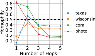
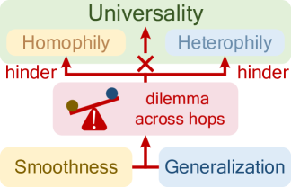
Figure 1. (a) Mixture of homophily and heterophily across multi-hop neighborhoods in real-world graphs. (b) Smoothness-generalization dilemma is the key factor hindering universality of homophily and heterophily.

Graph Neural Networks (GNNs) (Scarselli et al., 2008; Kipf and Welling, 2016; Velickovic et al., 2017; Hamilton et al., 2017; Gilmer et al., 2017) have attracted substantial attention in recent years, achieving notable success across various domains, such as transaction networks (Liu et al., 2021) and social networks (Fan et al., 2019). Most GNN models update a node’s representation by recursively aggregating information from its neighborhoods, typically within a $k$-hop subgraph, where $k$ is the number of GNN layers. Depending on the graph type, GNN methods are broadly classified into two categories: homophilic GNNs (homoGNNs) (Kipf and Welling, 2016; Velickovic et al., 2017; Hamilton et al., 2017; Gasteiger et al., 2018) and heterophilic GNNs (heteGNNs) (Zhu et al., 2020; Chien et al., 2020; Luan et al., 2022; Song et al., 2023). HomoGNNs operate under the homophily assumption, which posits that adjacent nodes tend to share similar labels (homophily). In contrast, heteGNNs are designed for heterophilic graphs, where connected nodes are more likely to have differing labels.

In practical graph applications, industry professionals typically rely on domain expertise to estimate the homophily ratio of graph data based on direct neighbors and then select state-of-the-art GNN methods accordingly. While straightforward, this approach can be restrictive, as the homophily ratio can vary significantly across different orders of neighboring nodes, as illustrated in Figure 1. For instance, in the Cora dataset, which is generally considered homophilic based on direct neighbors, homophily decreases sharply with increasing neighborhood order. Conversely, in the Texas dataset, typically classified as heterophilic, second-order neighbors exhibit high homophily. This variation complicates the application of models that rely solely on first-order neighbor information when aggregating data from different orders. This raises an important question: Can we develop a unified framework capable of simultaneously handling neighborhoods across varying orders and homophily ratios, thereby enabling universal processing of both homophilic and heterophilic graphs?

To answer this question, we first theoretically explore the message-passing process across multi-hop neighborhoods. Our analysis reveals a critical yet previously overlooked architectural aspect: the cascade dependency in multi-hop learning, where each hop’s representation is learned based on the preceding ones. We theoretically demonstrate that this cascade dependency leads to a smoothness-generalization dilemma across hops, as illustrated in Figure 1. In this context, smoothness refers to the ability of GNNs to bring closer node representations within specific neighborhoods, while the generalization indicates the model’s capability to adapt to varying neighborhood distribution shifts. In homophilic graphs, the dilemma has minimal effect on low-order neighborhoods as smoothing within homophilic neighborhoods coincides with strong generalization (Yang et al., 2022). However, it significantly hampers the learning of high-order neighborhoods due to the inevitable oversmoothing which is proved theoretically related to the dilemma. For heterophilic graphs, however, the negative effects are more pronounced across both low- and high-order neighborhoods. Effective generalization is consistently required to handle their more complex neighborhood class distributions, which are susceptible to distribution shifts caused by noise or sparsity, yet it is constrained by the imposed smoothness. This theoretical insight suggests that resolving the smoothness-generalization dilemma could benefit both homophilic and heterophilic settings without requiring separate treatment during learning, thereby breaking the paradox and improving the universality of GNNs.

To address this dilemma, we propose a universal message-passing framework called Inceptive Graph Neural Network (IGNN), which replaces the cascade dependency in multi-hop learning with an inceptive architecture that simultaneously learns from multiple receptive hops. We adopt the term inceptive (Szegedy et al., 2015) to denote a kind of architecture capturing information from multiple receptive fields concurrently. Our framework is built on three key principles: separative neighborhood transformation, inceptive neighborhoods aggregation and neighborhood relationship learning. First, IGNN learns independent representations for each hop through the separate transformations and inceptive architecture, decoupling the cascade dependency across hops. This enables personalized generalization capabilities for different hops, depending on their respective homophily ratios and smoothing levels. Second, IGNN enhances the independent representations by capturing neighborhood-wise relationships, allowing for the selection of the appropriate range of receptive fields. Moreover, the inceptive architecture is shown to facilitate the learning of a polynomial graph filter, benefiting universal settings by enabling the learning of arbitrary-pass filters.

In summary, the contributions of our work are as follows:

1. We provide a holistic theoretical understanding of the universality of GNNs: the newly discovered smoothness-generalization dilemma is a key factor hindering it, offering insights for theoretically supported universal designs.

2. We propose a simple yet universal framework, namely inceptive graph neural network (IGNN), designed to resolve this dilemma, benefiting both homophilic and heterophilic settings without the need for tailored designs for each.

3. Extensive experiments demonstrate that our IGNN outperforms 23 baseline methods. IGNN not only exhibits superior performance on both homophilic and heterophilic graphs, but also scales efficiently to large graphs.

2. Related Works

Homophilic Graph Neural Networks. Graph Neural Networks (GNNs) have demonstrated remarkable abilities in managing graph-structured data, particularly under the assumption of homophily. Traditional GNNs can be broadly categorized into two categories. Spectral GNNs, such as the Graph Convolutional Network (GCN) (Kipf and Welling, 2016), leverage various graph filters to derive node representations. In contrast, spatial GNNs aggregate information from neighboring nodes and combine it with the ego node to update representations, employing methods such as attention mechanisms (Velickovic et al., 2017) and sampling strategies (Hamilton et al., 2017). Unified frameworks (Ma et al., 2021; Zhu et al., 2021) have been proposed to integrate and elucidate these diverse message-passing approaches. Recent advancements have introduced multi-hop techniques to address the limitations of traditional GNNs in capturing long-range dependencies, with examples including skip connections (Hamilton et al., 2017), residual connections (Chen et al., 2020), and jumping knowledge mechanisms (Xu et al., 2018b). However, these methods primarily target homophilic graphs and are less effective when dealing with heterophilic graphs.

Heterophilic Graph Neural Networks. Addressing the challenges posed by heterophilic graphs, several innovative approaches have been proposed for graph neural networks. These include: (1) Neighborhood Extension: Techniques such as high-order neighborhood concatenation (Zhu et al., 2020), new neighborhood discovery (Pei et al., 2020), neighborhood refinement (Yan et al., 2022), and global information capture (Li et al., 2022). (2) Neighborhood Discrimination: Methods including ordered neighborhood encoding (Song et al., 2023), ego-neighbor separation (Zhu et al., 2020), and hetero-/homo-phily neighborhood separation (Pan and Kang, 2023). (3) Fine-Grained Information Utilization: Strategies such as multi-filter signal usage (Luan et al., 2022), intermediate layer combination (Zhu et al., 2020), and refined gating or attention mechanisms (Du et al., 2022). These methods generally retain the practice of message passing (Zheng et al., 2024), which involves aggregating multi-hop neighborhood information.

However, these methods often treat homophily and heterophily separately, leading to a paradox: effectively separating and handling them would require prior knowledge of node classes, which undermines the learning and prediction process. A holistic theoretical understanding is needed to address the factors hindering universality, guiding the development of an architecture that can seamlessly adapt to both homophily and heterophily without requiring different treatments during training.

3. Notations and Preliminaries

3.1. Notations

Given an undirected attribute graph $\mathcal{G}(\mathcal{V},\mathbf{X},\mathcal{E},\mathbf{A})$, the node set $\mathcal{V}=\{v_{1},v_{2},\cdots,v_{N}\}$ comprises $N$ nodes attributed with the feature matrix $\mathbf{X}=[\mathbf{x}_{0},\mathbf{x}_{1},\cdots,\mathbf{x}_{N}]^{\top}\in\mathbb{R}^{N\times D}$, while the edge set $\mathcal{E}$ is represented by the adjacency matrix $\mathbf{A}\in\mathbb{R}^{N\times N}$. $\mathbf{A}_{ij}=1$ if $(v_{i},v_{j})\in\mathcal{E}$, otherwise $\mathbf{A}_{ij}=0$. The degree matrix is denoted as $\mathbf{D}=\text{diag}(d_{1},d_{2},\cdots,d_{N})\in\mathbb{R}^{N\times N}$, with $d_{i}=\sum^{N}_{j}a_{ij}$ representing the degree of node $v_{i}$. Therefore, the re-normalization of the adjacency matrix $\widehat{\mathbf{A}}=\widehat{\mathbf{D}}^{-\frac{1}{2}}(\mathbf{\mathbf{A}}+\mathbf{I}_{N})\widehat{\mathbf{D}}^{-\frac{1}{2}}$, where $\mathbf{I}_{N}$ is the identity matrix. The symmetrically normalized graph Laplacian matrix is $\widehat{\mathbf{L}}=\mathbf{I}_{N}-\widehat{\mathbf{A}}$. Denote $\mathbf{C}=[\mathbf{c}_{1},\mathbf{c}_{2},\cdots,\mathbf{c}_{N}]\in\mathbb{R}^{N\times C}$ as the semantic labels of the nodes in one-hot format, and $C$ is the number of labels. As for the relationships between semantic labels and graph structures, edge homophily (Zhu et al., 2020) is computed as: $h_{e}=(1/|\mathcal{E}|)\sum_{(v_{i},v_{j})\in\mathcal{E}}\mathbb{I}(c_{i}=c_{j})$.

3.2. Preliminaries

3.2.1. Smoothness of GNNs

Oono and Suzuki (2019) describe the smoothness characteristic of GNNs with information loss from $\mathbf{X}$ in its research on asymptotic behaviors of GNNs from a dynamical systems perspective. They take into consideration all the non-linearity, convolution filters and linear transformation layers of the most typical message passing method GCN, and demonstrate that when it extends with more layers, the representation (i.e., $\mathbf{H}^{(k)}_{G}=\sigma(\widehat{\mathbf{A}}\mathbf{H}^{(k-1)}\mathbf{W}^{(k)})$, see Section 4.1 for detail) exponentially approaches information-less states, which they describe as a subspace $\mathcal{M}$ in Definition 3.1 that is invariant under the dynamics.

Definition 3.1 (subspace).

Let $\mathcal{M}:=\left\{\mathbf{E}\mathbf{B}\mid\mathbf{B}\in\mathbb{R}^{M\times D}\right\}$ be an $M$-dimensional subspace in $\mathbb{R}^{N\times D}$, where $\mathbf{E}\in\mathbb{R}^{N\times M}$ is orthogonal, i.e. $\mathbf{E}^{\mathrm{T}}\mathbf{E}=\mathbf{I}_{M}$, and $M\leq N$.

Following the notations in (Oono and Suzuki, 2019), we denote the maximum singular value of $\mathbf{W}^{(l)}$ by $s_{l}$ and set $s:=\sup_{l\in\mathbb{N}_{+}}s_{l}$. Denote the distance that induced as the Frobenius norm from $\mathbf{X}$ to $\mathcal{M}$ by $d_{\mathcal{M}}(\mathbf{X}):=\inf_{\mathbf{Y}\in\mathcal{M}}\|\mathbf{X}-\mathbf{Y}\|_{\mathrm{F}}=\mathcal{D}$. The following Corollary 3.2 can be interpreted as the information loss as layer $l$ goes.

Corollary 3.2 (Oono and Suzuki (2019)).

Let $\lambda_{1}\leq\cdots\leq\lambda_{N}$ be the eigenvalues of $\widehat{A}$, sorted in ascending order. Suppose the multiplicity of the largest eigenvalue $\lambda_{N}$ is $M(\leq N)$, i.e., $\lambda_{N-M}<\lambda_{N-M+1}=\cdots=\lambda_{N}$ and the second largest eigenvalue is defined as $\lambda:=\max_{n=1}^{N-M}\left|\lambda_{n}\right|<\left|\lambda_{N}\right|=1.$ Let $\mathbf{E}$ to be the eigenspace associated with $\lambda_{N-M+1},\cdots,\lambda_{N}$. Then we have $\lambda<\lambda_{N}=1$, and

(1) $$d_{\mathcal{M}}\left(\mathbf{H}^{(l)}\right)\leq s_{l}\lambda d_{\mathcal{M}}\left(\mathbf{H}^{(l-1)}\right),$$

where $\mathcal{M}:=\left\{\mathbf{E}\mathbf{B}\mid\mathbf{B}\in\mathbb{R}^{M\times D}\right\}$. Besides, if $s_{l}\lambda<1$, the output of the $l$-th layer of GCN on $\mathcal{G}$ exponentially approaches $\mathcal{M}$.

A smaller distance from the representations to the subspace $\mathcal{M}$ (i.e., $d_{\mathcal{M}}(\mathbf{H}^{(l)})$) indicates greater smoothness with larger information loss (Oono and Suzuki, 2019). This is because the subspace $\mathcal{M}$ denotes the convergence state of minimal information retained from the original node features $\mathbf{X}$ with the only information of the connected components and node degrees of $\widehat{\mathbf{A}}$. This means, as for any $\mathbf{Y}\in\mathcal{M}$, if two nodes $v_{i},v_{j}\in\mathcal{V}$ are in the same connected component and their degrees are identical, then the corresponding column vectors of $\mathbf{Y}$ are identical, meaning unable to distinguish them using $\mathbf{Y}$.

3.2.2. Generalization of GNNs

As discussed in existing works (Szegedy, 2013; Virmaux and Scaman, 2018; Khromov and Singh, 2024), a model’s generalization capability can be governed by the Lipschitz constant of the neural network as in Definition 3.3.

Definition 3.3 (Lipschitz constant).

A function $f:\mathbb{R}^{n}\rightarrow\mathbb{R}^{m}$ is called Lipschitz continuous if there exists a constant $L$ such that

(2) $$\forall x,y\in\mathbb{R}^{n},\|f(x)-f(y)\|_{2}\leq L\|x-y\|_{2},$$

where the smallest $L$ for which the previous inequality is true is called the Lipschitz constant of $f$ and will be denoted $\hat{L}$.

A smaller $L(f)$ means the GNN has better generalization capability (Tang and Liu, 2023). Please note that, this paper does not discuss the generalization ability on graph domain adaption (Liu et al., 2024). Instead, we discuss the generalization ability concerning inherent structural disparity (Mao et al., 2024) and data distribution shifts from the training set to the test set (Tang and Liu, 2023).

4. Methodology

4.1. Revisiting Message Passing

Generally, most graph neural networks (GNNs) capture multi-order neighborhood information by recursively stacking message-passing (MP) layers. This process is typically divided into two stages: the aggregation stage and the combination stage (Xu et al., 2018a):

(3) $$\mathbf{h}^{(0)}_{v}=\mathbf{x}_{v},$$

(4) $$\mathbf{m}^{(k)}_{v}=\text{AGG}^{(k)}(\{\mathbf{h}^{(k-1)}_{u}\mid u\in\mathcal{N}(v)\}),$$

(5) $$\mathbf{h}^{(k)}_{v}=\text{COM}^{(k)}(h_{v}^{(k)},m_{v}^{(k)}),$$

where $\mathbf{h}_{v}^{(k)}$ is the hidden representation and $\mathbf{m}^{(k)}_{v}$ is the message for node $v$ in the $k$-th layer. Here, $\mathcal{N}(v)$ denotes the set of neighbors adjacent to node $v$, while $\text{AGG}(\cdot)$ and $\text{COM}(\cdot)$ represent the aggregation and combination function, respectively. Denoting $\mathbf{H}^{(k)}=[\mathbf{h}_{0}^{(k)},\mathbf{h}_{1}^{(k)},\cdots,\mathbf{h}_{N}^{(k)}]^{\top}\in\mathbb{R}^{N\times F}$, the most widely used GCN implementation can be written as $\mathbf{H}^{(k)}_{G}=\sigma(\widehat{\mathbf{A}}\mathbf{H}^{(k-1)}\mathbf{W}^{(k)})$, where $\sigma(\cdot)$ is the activation function.

4.1.1. Smoothness-Generalization Dilemma

Obtaining information from a $k$-hop neighborhood typically requires $k$ layers of MP. Despite its computational efficiency (Kipf and Welling, 2016), it introduces an unexpected limitation. The following Theorem 4.1 reveals a dilemma between the smoothness and generalization ability. Please refer to Appendix  A.1 for the proof.

Theorem 4.1.

Given a graph $\mathcal{G}(\mathbf{X},\mathbf{A})$, let the representation obtained via $k$ rounds of GCN message passing on symmetrically normalized $\widehat{\mathbf{A}}$ be denoted as $\mathbf{H}^{(k)}_{G}=\sigma(\widehat{\mathbf{A}}\mathbf{H}^{(k-1)}\mathbf{W}^{(k)})$, and the Lipschitz constant of this $k$-layer graph neural network be denoted as $\hat{L}_{G}$. Given the distance from $\mathbf{X}$ to the subspace $\mathcal{M}$ as $d_{\mathcal{M}}(\mathbf{X})=\mathcal{D}$, then the distance from $\mathbf{H}^{(k)}_{G}$ to $\mathcal{M}$ satisfies:

(6) $$d_{\mathcal{M}}(\mathbf{H}_{G}^{(k)})\leq\hat{L}_{G}\lambda^{k}\mathcal{D},$$

where $\hat{L}_{G}=\|\prod_{i=0}^{k}\mathbf{W}^{(i)}\|_{2}$, and $\lambda<1$ is the second largest eigenvalue of $\widehat{\mathbf{A}}$.

Corollary 4.2.

$\forall\hat{L}_{G},\epsilon>0,\exists k^{*}=\lceil{(\log\frac{\epsilon}{\hat{L}_{G}\mathcal{D}})/\log\lambda}\rceil$, such that $d_{\mathcal{M}}(\mathbf{H}_{G}^{(k^{*})})<\epsilon$, where $\lceil{\cdot}\rceil$ is the ceil of the input.

Remark. As $\mathcal{D}$ is constant with respect to $\mathbf{X}$, we observe that the distance is upper-bounded by three factors: the second largest eigenvalue $\lambda$ of $\widehat{{\mathbf{A}}}$, the Lipschitz constant $\hat{L}_{G}$ corresponding to the norm of the product of all weight matrices $\mathbf{W}^{(i)}$, and the layer depth $k$. Based on this, several conclusions can be drawn.

First, there exists a dilemma between the smoothness and generalization ability of the network, which leads to a performance drop as layer depth increases. From Section 3.2.1, we know that a smaller distance to $\mathcal{M}$ indicates greater smoothness with information loss. The state of extremely small distance with indistinguishable representations is referred to as oversmoothing. Since $\lim_{k\rightarrow\infty}\lambda^{k}=0$, $\hat{L}_{G}$ has to rise when $k$ increases to prevent $d_{\mathcal{M}}(\mathbf{H}_{G}^{(k)})$ from converging into $0$. This is evidenced by the upper bound of the Lipschitz constant continuing to increase as training progresses (Khromov and Singh, 2024) However, a large $\hat{L}_{G}$ implies reduced generalization, leading to a significant performance gap between training and test accuracy (Tang and Liu, 2023). Consequently, either oversmoothing or poor generalization will occur at large $k$.

Second, oversmoothing is inevitable in high-order neighborhoods within the GCN message-passing framework. From Corollary 4.2, we see that for any given $\hat{L}_{G}$, there exists a $k$ such that the distance from the representations to the subspace $\mathcal{M}$ is smaller than any arbitrarily small $\epsilon$. Thus, oversmoothing becomes unavoidable for sufficiently large $k$, as $\hat{L}_{G}$ computing from the learning parameter weight matrices can not be infinitely large.

Note that several works (Oono and Suzuki, 2019; Rong et al., 2019; Chen et al., 2020) have analyzed the inevitability of oversmoothing in GNNs. However, they primarily focus on oversmoothing itself and fail to connect it with generalization. Our work is the first to elucidate the dilemma between smoothness and generalization by proposing a tighter upper bound for $d_{\mathcal{M}}(\mathbf{H}_{G}^{(k)})$ that bridges these concepts.

4.1.2. Dilemma Hinders Universality of GNNs

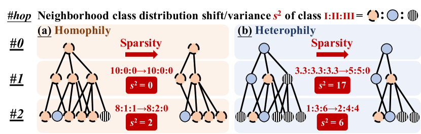
Figure 2. Neighborhood class distribution (NCD) shifts caused by the same sparsity. (a) Homophilic graphs calls for more smoothness, as small variance ($s^{2}$) indicates less distribution shift. (b) Heterophilic graphs require stronger model generalization capability to mitigate the larger shifts they experience due to their more complex NCDs.

This dilemma has significant negative implications for the universality of GNNs, as analyzed through both homophilic and heterophilic settings below.

In homophilic settings, the dilemma primarily affects high-order neighborhoods through inevitable oversmoothing, whereas low-order neighborhoods are less impacted. This can be intuitively understood by recognizing that in low-order homophilic neighborhoods, smoothing and generalization are aligned, as message passing pulls together the representations of nodes with the same label, which is beneficial. However, in high-order neighborhoods with lower homophily, smoothing begins to conflict with generalization, as bringing nodes from different classes closer together is detrimental. This is evidenced by a recent work, PMLP (Yang et al., 2022), which is equivalent to an MLP during training but exhibits significantly better generalization after adding an untrained message-passing layer during testing on homophilic graphs, rivaling its GNN counterpart in most cases. Nevertheless, when applied to sufficiently large-order neighborhoods, PMLP also experiences the same performance degradation as other GNNs due to inevitable oversmoothing (Yang et al., 2022).

In heterophilic settings, the dilemma exhibits its negative effects across both low-order and high-order neighborhoods. This can be explained from two perspectives. First, the complex neighborhood class distribution (NCD) (Ma et al., 2022) in heterophilic graphs makes it easy for noise or even inherent sparsity to result in mismatched or incomplete NCDs for nodes of the same class, which requires strong generalization ability to mitigate. A toy example in Figure 2 demonstrates that heterophilic graphs suffer from larger neighborhood class distribution shifts caused by the same graph sparsity compared to homophilic graphs, as evidenced by larger distribution variances even in first-order neighborhoods. This makes heterophilic graphs more prone to neighborhood inconsistencies across all neighborhoods, thus requiring stronger generalization. Second, there is a greater structural inconsistency between the training and test sets in heterophilic graphs compared to homophilic ones, as heterophilic graphs exhibit a mixture of homophilic and heterophilic patterns (Mao et al., 2024), which requires good generalization to align performance between training and testing. Mao et al. (2024) investigates how the structural disparity resulting from the mixture of homophily and heterophily contributes to performance gaps in GNNs, emphasizing that generalization is critical for heterophilic GNNs. In all, the aforementioned two characteristics of heterophily both demand strong generalization ability, while the inevitable smoothing effects of message passing ask for a large Lipschitz constant to prevent excessive information loss, which, in turn, leads to unexpectedly poor generalization.

In summary, the core insight is that this dilemma hinders GNN performance in both homophilic and heterophilic settings, ultimately contributing to the absence of universality.

4.2. Proposed Inceptive Message Passing Framework

To address the aforementioned dilemma, we propose a new message-passing architecture called Inceptive Message-Passing Graph Neural Networks (IGNN). Rather than introducing new modules into the original message-passing framework, this architecture transforms its cascade-dependent structure into an inceptive one. Our experiments in Section 5 demonstrate that IGNN, even with the simplest vanilla GCN aggregation, outperforms all baselines across both homophilic and heterophilic datasets, confirming that the dilemma is indeed the fundamental issue limiting the universality of GNNs.

4.2.1. Inceptive GNNs (IGNN)

Our proposed framework highlights three simple yet effective principles to form an inceptive GNN: (1) Separative Neighborhood Transformation; (2)Inceptive Neighborhood Aggregation; and (3) Relative Neighborhood Learning.

Separative Neighborhood Transformation (SN)

The key is to avoid sharing or coupling transformation layers across neighborhoods:

(7) $$\mathbf{h}^{(k)}_{v}=f^{(k)}(\mathbf{x}_{v})=\mathbf{x}_{v}\mathbf{W}^{(k)},$$

where $f^{(k)}(\cdot)$ represents the transformation for the $k$-th neighborhood. The absence of SN implies all $k$-hop neighborhood transformations either share the same parameters $\mathbf{W}_{\theta}$ or are cascade-coupled in a multiplicative manner, such as $\prod_{i}^{k}\mathbf{W}^{i}$, as shown in Table 1. This design aims to capture the unique characteristics of each neighborhood and decouple their learning processes, enabling personalized generalization with distinct Lipschitz constants for different neighborhoods. This is crucial, as various hops exhibit different levels of homophily (Ai et al., 2024).

Table 1. Comparison of inceptive GNNs variants. The following notations are used only to illustrate the relevant forms and do not necessarily conform to the actual expressions. $\gamma_{k}$ denotes learnable coefficients, and $K$ is the network depth. $\textit{s}(\cdot)$ refers to the softmax function, while $g(\cdot)$ represents the ordered gating attention function. $\mathbf{W}_{a}$ is the weight matrix for the attention, and $\mathbf{W}_{I}/\mathbf{W}_{L}/\mathbf{W}_{H}/\mathbf{W}_{\text{mix}}$ denote weight matrices of full-/low-/high-pass/mixed signals, respectively.

Model	Subtype	$\mathbf{W}$ of $k$-th hop	weight of $k$-th hop
APPNP	Residual	$\mathbf{W}_{\theta}$	$\alpha(1-\alpha)^{k},$ $(1-\alpha)^{K},\alpha\in(0,1]$
JKNet	Concatenative	$\prod_{i=0}^{k}\mathbf{W}^{(i)}$	—
IncepGCN	Concatenative	$\prod_{i=0}^{k}\mathbf{W}^{(i)}$	—
SIGN	Concatenative	$\mathbf{W}^{(k)}$	—
MixHop	Concatenative	$\mathbf{W}^{(k)}$	—
DAGNN	Attentive	$\mathbf{W}_{\theta}$	$\sigma(\widehat{\mathbf{A}}^{k}\mathbf{X}\mathbf{W}_{\theta}\mathbf{W}_{a})$
GCNII	Residual	$\prod_{i=K-k+1}^{K}\mathbf{W}^{(i)}$	implicit $\gamma_{k}$
GPRGNN	Attentive	$\mathbf{W}_{\theta}$	explicit $\gamma_{k}$
ACMGCN	Attentive	$\left(\prod_{i=0}^{k}\mathbf{W}_{L/H}^{(i)}\cdot\right.$ $\left.\prod_{i=K-k+1}^{K}\mathbf{W}_{I}^{(i)}\right)$	$\textit{s}\left(([\mathbf{H}_{I/L/H}^{(k)}\mathbf{W}_{I/L/H}^{(k)}]/T)\right.$ $\left.\mathbf{W}_{\text{mix}}^{(k)}\right)$
OrderedGNN	Attentive	$\mathbf{W}_{\theta}$	$g(\mathbf{m}_{v}^{(k)},\mathbf{h}_{v}^{(k-1)})$
IGNN	Concatenative	$\mathbf{W}^{(k)}$	implicit $\gamma_{k}$

Inceptive Neighborhood Aggregation (IN)

This core design simultaneously embeds different receptive fields, such as various hops or customized relational neighborhoods:

(8) $$\mathbf{m}^{(k)}_{v}=\text{{AGG}}^{(k)}\left(\{\mathbf{h}_{u}^{(k)}\mid u\in\mathcal{N}^{(k)}_{v}\}\right),$$

where $\text{{AGG}}(\cdot)$ represents the neighborhood aggregation function for each neighborhood, or in other words, the receptive field. The simplest approach involves partitioning the $k$-th order rooted tree of neighborhoods into $k$ distinct neighborhoods $\mathcal{N}_{v}^{(k)}=\mathcal{N}_{v}(\mathbf{A}^{k})$ with $\mathcal{N}^{(0)}_{v}=\{v\}$. Additionally, neighborhoods identified through techniques such as structure learning can be incorporated into this framework as customized relational neighborhoods. The inceptive nature of the architecture prevents higher-order neighborhood representations from being computed based on lower-order ones, i.e., $\mathbf{m}^{(k)}_{v}=\psi(\mathbf{h}^{(k-1)}_{v})$ as in Equation (4). This avoids cascading the learning of different hops, which could propagate errors across all hops if one becomes corrupted. Moreover, it prevents the product-type amplification of the Lipschitz constant, as described in 4.1, which would otherwise limit the network’s generalization ability.

Neighborhood Relationship Learning (NR)

Up to this stage, all $\mathbf{m}_{v}^{(k)}$ are learned separately. Therefore a neighborhood-wise relationship learning module is added to learn the correlations among neighborhoods, including their commonalities or differences:

(9) $$\mathbf{h}_{v}=\text{\text{{REL}}}\left(\{\mathbf{m}_{v}^{(k)}\mid 0\leq k\leq K\}\right),$$

where $\text{{REL}}(\cdot)$ is the relationship learning function of multiple neighborhoods. The relationships among different neighborhoods represent a new characteristic in our framework compared to original framework while the ego feature is included as $\mathbf{m}^{(0)}$.

Various relationships can be learned through diverse techniques, such as concatenation with learnable transformation (Hamilton et al., 2017), deep set embedding with mean/max/sum pooling (Zaheer et al., 2017), and attention like ordered gating mechanism (Song et al., 2023), etc., can be applied. Based on the mechanism selected, IGNN can be divided into three variants: concatenative, residual and attentive IGNN-s. These methods are typically considered different, but we will show their consistency as variants of inceptive GNNs below.

4.2.2. Variants of IGNNs

Here, we demonstrate that several seemingly unrelated network structure designs in GNNs surprisingly create an inceptive variant, with a brief comparison in Table 1. From the success of these various architectures in their own fields, we can indirectly realize the importance of introducing inceptive architectures to the universality of GNNs.

Residual IGNN

Residual connection (He et al., 2016) is a widely used technique to train deep neural networks. Kipf and Welling (2016) first leverage it in vanilla GCN as: $\mathbf{H}^{(k)}=\sigma(\widehat{\mathbf{A}}\mathbf{H}^{(k-1)}\mathbf{W}^{(k)})+\mathbf{H}^{(k-1)}$. It is easy to observe that the expansion expression of the $\mathbf{H}^{(k)}$ will cover all $\widehat{\mathbf{A}}^{i},1<i<k$, which is an inceptive variant with an IN design. Besides, some methods (Gasteiger et al., 2018; Chen et al., 2020) adopt an initial residual connection, constructing connections to the initial representation $\mathbf{H}^{(0)}$: $\mathbf{H}^{(k)}=\sigma(\widehat{\mathbf{A}}\mathbf{H}^{(k-1)}\mathbf{W}^{(k)})+\mathbf{H}^{(0)}$, where $\mathbf{H}^{(0)}=\sigma(\mathbf{X}\mathbf{W}^{(0)})$. Leaving out all non-linearity for simplicity, we can derive the expression for $\mathbf{H}^{(k)}$ in terms of $\mathbf{X}$ as: $\mathbf{H}^{(k)}=\sum_{i=0}^{k}\widehat{\mathbf{A}}^{k-i}\mathbf{X}\mathbf{W}^{(0)}(\prod_{j=i+1}^{k}\mathbf{W}^{(j)})$, where $\prod_{i=k+1}^{k}\mathbf{W}^{(j)}=\mathbf{I}$. This formulation is also an inceptive variant of IN design. However, these two variants still involve a large number of cascade-coupled weight matrix multiplications for either low- or high-order neighborhoods, which may suffer from the aforementioned dilemma.

Attentive IGNN

Different from the above variant, attentive IGNN-s leverage the attention mechanism to realize node-wise personalized neighborhood relationship learning, defined as:

(10) $$\mathbf{h}_{v}^{(k)}=\alpha_{0}^{(k)}\mathbf{m}_{v}^{(k)}+\alpha_{1}^{(k)}\mathbf{h}_{v}^{(k-1)},$$

where $\alpha_{i}^{(k)}=g_{i}(\mathbf{m}_{v}^{(k)},\mathbf{h}_{v}^{(k-1)})$, $i\in\{1,2\}$. $g(\cdot)$ is the mechanism function. Several methods such as DAGNN (Liu et al., 2020), GPRGNN (Chien et al., 2020), ACMGCN (Luan et al., 2022) and OrderedGNN (Song et al., 2023) all incorporate this attentive architecture through different attention mechanism design to realize the IN and NR design. However, as can be seen from Table 1, these methods either share the same $\mathbf{W}_{\theta}$ across all neighborhoods or cascade couple the weight matrices of different hops, which is unable to allow distinct Lipschitz constant for their sub-networks to adapt to their different extent of smoothness.

Concatenative IGNN

This variant is defined as a concatenation of multi-neighborhood messages with a learnable transformation:

(11) $$\mathbf{h}_{v}=\sigma\left((||_{i=0}^{k}\sigma(\mathbf{m}_{v}^{(k)}))\mathbf{W}\right),$$

where $||$ is the concatenation operator. Although simple, its power is surprisingly strong, as it can achieve various relationships with learnable parameters, such as mean or sum neighborhood pooling, and even more complex relationships found in existing methods, like the general layer-wise neighborhood mixing of MixHop (Abu-El-Haija et al., 2019), personalized PageRank (PPR) of APPNP (Gasteiger et al., 2018), and Generalized PageRank (GPR) weights of GPRGNN (Chien et al., 2020)  (see Proof A.3). It is worth noting that, the exact simple architecture has been widely adopted by many previous works targeting various problems other than heterophily, such as MixHop (Abu-El-Haija et al., 2019) for layer-wise neighborhood mixing, SIGN (Frasca et al., 2020) for scalability improvement, and IncepGCN (Rong et al., 2019) for over-smoothing. However, surprisingly, no one has discovered their consistent effectiveness in heterophilic/universality graph learning.

4.2.3. Putting All Together: Simplest IGNN

Taking vanilla GCN aggregation as AGG($\cdot$) and concatenation with learnable transformation as REL($\cdot$), the simplest variant of IGNN is defined as:

(12) $$\mathbf{h}_{v}^{(k)}=\mathbf{x}_{v}\mathbf{W}^{(k)},$$

(13) $$\mathbf{m}_{v}^{(k)}=\sum_{u}\sigma(\widehat{\mathbf{A}}_{v,u}^{k}\mathbf{h}_{u}^{(k)}),$$

(14) $$\mathbf{h}_{v,k}=\sigma\left((||_{i=0}^{k}\sigma(\mathbf{m}_{v}^{(k)}))\mathbf{W}\right),$$

where $\widehat{\mathbf{A}}^{0}=\mathbf{I}$. Its matrix format is $\mathbf{H}_{IG,k}=\sigma((||_{i=0}^{k}\sigma(\widehat{\mathbf{A}}^{i}\mathbf{X}\mathbf{W}^{(i)}))\mathbf{W}),$ where $\mathbf{W}^{(i)}\in\mathbb{R}^{D\times F}$, and $\mathbf{W}\in\mathbb{R}^{kF\times F^{\prime}}$. Unless otherwise stated, all IGNN below refers to this simplest implementation.

4.3. How Can IGNN Benefit Universality

Here, we theoretically demonstrate the universality of IGNN.

4.3.1. Eliminating the Smoothness-Generalization Dilemma across Hops.

As theoretically analyzed in Section 4.1.2, the inherent dilemma in original message-passing framework will hinder the universality of GNNs in different ways for homophilic and heterophilic settings. The following Theorem 4.3 shows that IGNN can release the dilemma and thus benefit both settings for improving universality.

Theorem 4.3.

Given a graph $\mathcal{G}(\mathbf{X},\mathbf{A})$, let the representation of IGNN be denoted as $\mathbf{H}_{IG,k}=\sigma((||_{i=0}^{k}\sigma(\widehat{\mathbf{A}}^{i}\mathbf{X}\mathbf{W}^{(i)}))\mathbf{W})$, and the Lipschitz constant of it be denoted as $\hat{L}_{IG}$. Given the distance from $\mathbf{X}$ to the subspace $\mathcal{M}$ as $d_{\mathcal{M}}(\mathbf{X})=\mathcal{D}$ and $\mathbf{W}=\left[\begin{smallmatrix}\mathbf{W}_{0}\\ \cdots\\ \mathbf{W}_{k}\end{smallmatrix}\right]$, then the distance from $\mathbf{H}_{IG,k}$ to $\mathcal{M}$ satisfies:

(15) $$d_{\mathcal{M}}(\mathbf{H}_{IG,k})\leq\left\|\sum_{i=0}^{k}\lambda^{i}\mathbf{W}^{(i)}\mathbf{W}_{i}\right\|_{2}\mathcal{D},$$

where $\lambda<1$ is the second largest eigenvalue of $\widehat{\mathbf{A}}$, and $\hat{L}_{IG}=\|\sum_{i=0}^{k}\mathbf{W}^{(i)}\mathbf{W}_{i}\|_{2}$.

Remark. Theorem 4.3 demonstrates the effective elimination of the dilemma from two perspectives. From the global perspective, the overall Lipschitz constant of the entire network is effectively shrunk to avoid an extreme decrease in the generalization of the network. It is a cascade multiplication $\hat{L}_{G}=\|\prod_{i=0}^{k}\mathbf{W}^{(i)}\|_{2}$ in the message passing framework, which will grow exponentially as the layer depth increases since each high-order neighborhoods suffering from oversmoothing all demand large $\hat{L}_{G}$, and the cascade multiplication will lead to excessive growth in magnitude. While the Lipschitz constant is a summation of individual multiplication of various two terms in IGNN, whose increase in magnitude will be much smaller than that of cascade multiplication. From the local perspective, a more flexible personalized trade-off between smoothness and Generalization is enabled for each neighborhood. Since IGNN gives each neighborhood isolated transformation layers, making it possible to learn individual sub-network Lipschitz constant for their distinct magnitude of $\lambda^{k}$ and homophily level (Ai et al., 2024). High-order neighborhoods with extremely small $\lambda^{k}$ demand a large Lipschitz constant to mitigate information loss, while low-order or homophilic ones with relatively large $\lambda^{k}$ can enjoy sufficient small Lipschitz constant to guarantee the generalization of robustness of their representations.

4.3.2. Adaptive Graph Filters

Many existing works has highlighted the significance of high-frequency signals for heterophilic graph learning (Luan et al., 2022; Bo et al., 2021). Different from their practice of designing hand-crafted high-pass and low-pass filters, IGNN has the ability to adaptively learn arbitrary-pass graph filters. Despite the simple architecture, IGNN has expressive power beyond the polynomial graph filters (Defferrard et al., 2016) as in Theorem 4.4. See proof in Appendix A.2.

Theorem 4.4.

One layer of a $K$-hop concatenative IGNN, i.e., $\mathbf{H}=\sigma((||_{i=0}^{K}\sigma(\widehat{\mathbf{A}}^{i}\mathbf{X}\mathbf{W}^{(i)}))\mathbf{W})$), can express a $K$ order polynimial graph filter ($\sum_{i=0}^{K}\theta_{i}\widehat{\mathbf{L}}^{i}$) with arbitrary coefficients $\theta_{i}$.

Remark. Theorem 4.4 shows that IGNN can achieve a $K$-order polynomial graph filter, which can be viewed as a simplified case of it. Since polynomial graph filters have been proven able to approximate any graph filter (Shuman et al., 2013), this suggests that IGNN can learn arbitrary graph filters without the need for manually designing low-pass or high-pass filters. Apart from the capability of polynomial graph filters, several existing polynomial graph filter-like methods can also be achieved through simplified cases of IGNN, which can be seen in the following propositions. For proofs see Appendix A.3.

Proposition 4.5.

The Personalized PageRank of APPNP and Generalized PageRank of GPRGNN can all be achieved with simplified cases of IGNN.

Proposition 4.6.

SIGN, APPNP, MixHop, and GPRGNN are not as expressive as IGNN, as they can be viewed as simplified cases of it.

5. Experiments

In this section, we aim to answer the following research questions through extensive experiments on multiple real-world datasets:

• RQ1: How does the proposed IGNN method perform compared to the state-of-the-art methods?

• RQ2: What are the contributions of the three principles?

• RQ3: How is the dilemma resolved crossing different neighborhood orders?

Table 2. Baselines. Homo. and Hetero. mean homophilic and heterophilic. Non., and Incep. are non-inceptive and inceptive.

Type	Subtype	Model
Graph-agnostic		MLP
Homo. GNNs	Non.	GCN (Kipf and Welling, 2016), SGC (Wu et al., 2019), GAT (Velickovic et al., 2017), GraphSAGE (Hamilton et al., 2017)
	Incep.	APPNP (Gasteiger et al., 2018), SIGN (Frasca et al., 2020), IncepGCN (Rong et al., 2019), JKNet (Xu et al., 2018b), MixHop (Abu-El-Haija et al., 2019), DAGNN (Liu et al., 2020), GCNII (Chen et al., 2020)
Hetero. GNNs	Non.	H2GCN (Zhu et al., 2020), GBKGNN (Du et al., 2022), GGCN (Yan et al., 2022), GloGNN (Li et al., 2022), HOGGCN (Wang et al., 2022),
	Incep.	GPRGNN (Chien et al., 2020), ACMGCN (Luan et al., 2022), OrderedGNN (Song et al., 2023)
Graph Transformer		NodeFormer (Wu et al., 2022) DIFFormer (Wu et al., 2023a) SGFormer (Wu et al., 2023b)

Table 3. Overall performance of node classification on ten datasets. The best results are in bold, and the second-best results are underlined. A.R denotes the average of all baseline ranks computed across all datasets. OOM means out of memory.

Dataset	Actor	Blog	Flickr	Roman-E	Squirrel-f	Chame-f	Amazon-R	Pubmed	Photo	Wikics	A.R.
$h_{e}$	0.2163	0.4011	0.2386	0.0469	0.2072	0.2361	0.3804	0.8024	0.8272	0.6543
#Nodes	7,600	5,196	7,575	22,662	2,223	890	24,492	19,717	7,650	11,701
#Edges	33,544	171,743	239,738	32,927	46,998	8,854	93,050	44,338	238,162	431,206
#Feats	931	8,189	12,047	300	2,089	2,325	300	500	745	300
#Classes	5	6	9	18	5	5	5	3	8	10
MLP	34.69±0.71	93.08±0.63	89.41±0.73	62.12±1.79	34.00±2.44	35.00±3.29	42.25±0.73	87.68±0.51	86.73±2.20	73.51±1.18	20.6
SGC	29.46±0.96	72.85±1.15	59.02±1.48	42.90±0.50	39.75±1.85	42.42±3.28	41.32±0.80	87.14±0.57	92.38±0.49	77.63±0.88	18.9
GCN	30.82±1.41	77.28±1.43	69.06±1.70	36.23±0.57	37.06±1.42	41.46±3.42	44.96±0.40	87.70±0.58	94.88±2.08	78.59±1.07	18.2
GAT	30.94±0.95	85.36±1.37	57.87±2.22	62.31±0.93	38.22±1.41	40.69±3.20	47.41±0.80	87.64±0.54	94.72±0.52	76.92±0.81	18.2
GraphSAGE	34.52±0.64	95.73±0.53	91.74±0.58	66.39±2.16	34.83±2.24	41.24±1.65	46.71±2.83	88.71±0.65	94.52±1.27	80.85±1.00	15.4
APPNP	35.09±0.79	96.13±0.58	91.21±0.52	71.76±0.34	34.18±1.68	41.12±3.25	47.72±0.54	87.97±0.62	95.05±0.43	83.04±0.94	14.2
JKNet-GCN	30.49±1.71	84.25±0.71	71.72±1.47	69.61±0.42	40.11±2.54	43.31±3.12	48.15±0.93	87.41±0.38	94.39±0.40	83.80±0.65	14.9
IncepGCN	35.69±0.75	96.67±0.48	90.42±0.71	80.97±0.49	38.27±1.36	43.31±2.18	52.72±0.80	89.32±0.47	95.66±0.40	85.22±0.48	7.0
SIGN	36.76±1.00	96.06±0.68	91.81±0.58	81.56±0.57	42.13±1.99	44.66±3.46	52.47±0.95	90.29±0.50	95.53±0.43	85.59±0.79	4.4
MixHop	36.82±0.98	96.05±0.48	89.78±0.63	79.39±0.40	41.35±1.04	44.61±3.16	47.91±0.53	89.40±0.37	94.91±0.45	83.15±0.96	9.3
DAGNN	35.04±1.03	96.73±0.61	92.18±0.73	73.94±0.45	35.62±1.48	40.96±2.91	50.44±0.52	89.76±0.55	95.70±0.40	85.07±0.73	8.7
GCNII	35.69±1.08	96.25±0.61	91.36±0.68	80.55±0.82	37.96±2.49	42.13±2.04	47.65±0.48	90.00±0.46	95.54±0.34	85.15±0.56	8.3
H2GCN	32.74±1.23	96.32±0.62	91.33±0.59	68.70±1.66	33.89±1.01	38.09±2.63	36.65±0.73	89.50±0.43	91.56±1.49	74.76±3.39	17.4
GBKGNN	35.74±4.46	OOM	OOM	66.10±4.61	34.58±1.63	41.52±2.36	41.00±1.62	88.66±0.43	93.39±2.00	81.85±1.83	18.3
GGCN	35.72±1.48	96.09±0.55	90.17±0.76	OOM	35.62±1.52	38.54±3.99	OOM	89.19±0.43	95.32±0.27	83.67±0.75	15.4
GloGNN	35.82±1.27	92.53±0.80	88.18±0.85	70.87±0.89	35.39±1.70	40.28±2.91	49.01±0.74	88.14±0.25	92.15±0.33	84.20±0.55	15.3
HOGGCN	36.05±1.06	95.79±0.59	90.40±0.64	OOM	35.10±1.81	38.43±3.66	OOM	OOM	94.48±0.50	83.57±0.63	17.6
GPRGNN	35.79±1.04	96.26±0.62	91.52±0.56	72.36±0.38	36.92±1.24	41.63±2.86	46.07±0.78	89.45±0.61	95.51±0.39	83.16±1.23	10.9
ACMGCN	35.68±1.17	96.01±0.53	68.63±1.87	72.58±0.35	37.60±1.70	43.03±3.08	50.51±0.66	89.95±0.50	92.35±0.39	84.13±0.66	12.1
OrderedGNN	36.95±0.85	96.39±0.69	91.13±0.59	82.65±0.91	36.27±1.95	42.13±3.04	51.58±0.99	90.01±0.40	95.87±0.24	85.60±0.77	5.6
NodeFormer	36.10±1.09	94.28±0.67	89.05±0.99	70.24±1.58	38.38±1.81	38.93±3.68	42.67±0.77	88.36±0.43	93.81±0.75	80.98±0.84	15.3
DIFFormer	36.13±1.19	96.50±0.71	90.86±0.58	79.36±0.54	41.12±1.09	41.69±2.96	49.33±0.97	88.90±0.47	95.67±0.29	84.27±0.75	7.9
SGFormer	37.36±1.11	96.98±0.59	91.62±0.55	75.71±0.44	42.22±2.45	44.44±3.01	51.60±0.62	89.75±0.44	95.84±0.41	84.72±0.72	4.3
IGNN	38.71±1.00	97.13±0.21	93.23±0.61	86.07±0.60	43.89±1.79	47.13±5.18	53.01±0.77	90.29±0.41	95.75±0.38	86.09±0.48	1.2

Table 4. Overall performance of node classification on large datasets. The best results are in bold.

Dataset	ogbn-arxiv	pokec	ogbn-products
$h_{e}$	0.66	0.44	0.81
#Nodes	169,343	1,632,803	2,440,029
#Edges	1,166,243	30,622,564	123,718,280
#Feats	100	65	100
#Classes	40	2	47
MLP	55.50±0.23	63.27±0.12	61.06±0.12
GCN	71.74±0.29	74.45±0.27	75.45±0.16
GAT	71.74±0.29	72.77±3.18	79.45±0.28
SGC	70.74±0.29	73.77±3.18	74.78±0.17
SIGN	70.28±0.25	77.98±0.14	77.60±0.13
GPRGNN	71.40±0.32	78.62±0.15	78.23±0.25
NodeFormer	67.72±0.52	70.12±0.42	71.23±1.40
DIFFormer	69.85±0.34	72.89±0.56	74.16±0.32
SGFormer	72.62±0.18	73.24±0.54	76.24±0.45
IGNN	73.25±0.27	81.35±0.34	80.34±0.45

Table 5. Ablation of Three Principles. A.R. denotes denotes the average of all variants ranks computed across all dataset.

	GCN AGG($\cdot$)+			Equivalent	actor	blogcatalog	flickr	Roman-E	squirrel	chameleon	amazon-R	pubmed	photo	wikics	A.R.
	SN	IN	NR	Variant
1				GCN	30.82±1.41	77.28±1.43	69.06±1.70	36.23±0.57	37.06±1.42	41.46±3.42	44.96±0.40	87.70±0.58	94.88±2.08	78.59±1.07	5.7
2		✓			36.32±1.03	96.89±0.29	91.81±0.76	79.77±0.95	42.52±2.52	44.10±4.24	51.72±0.69	89.63±0.54	95.74±0.41	85.67±0.70	2.8
3			✓	JKNet+GCN	30.49±1.71	84.25±0.71	71.72±1.47	69.61±0.42	40.11±2.54	43.31±3.12	48.15±0.93	87.41±0.38	94.39±0.40	83.80±0.65	5.2
4	✓	✓		SIGN	36.76±1.00	96.06±0.68	91.81±0.58	81.51±0.38	42.13±1.99	44.66±3.46	52.47±0.95	90.29±0.50	95.53±0.43	85.59±0.79	2.8
5		✓	✓		36.63±1.17	96.54±0.48	90.75±0.84	83.86±0.59	42.16±1.93	42.87±4.66	51.58±0.82	89.22±0.45	95.54±0.42	85.04±0.83	3.5
6	✓	✓	✓	IGNN	38.71±1.00	97.13±0.21	93.23±0.61	86.07±0.60	43.89±1.79	47.13±5.18	53.01±0.77	90.30±0.41	95.79±0.43	86.09±0.48	1.0

5.1. Datasets, Baselines and Experiment Settings

Datasets. Following recent works (Luan et al., 2024), we select 13 representative datasets of various sizes up to millions of nodes, excluding those too small or too class-imbalanced (Zheng et al., 2024), as follows: (i) Heterophily: Roman-empire, BlogCatalog, Flickr, Actor (a.k.a., Film), Squirrel-filtered, Chameleon-filtered, Amazon-ratings, Pokec; (ii) Homophily: PubMed, Photo, wikics, ogbn-arxiv, ogbn-products. The Statistics of the datasets can be found in Table 3 and 4.

Baselines. We selected 23 representative baseline models, as shown in Table 2. These models are categorized into four main types: Graph-agnostic base models, Homophilic GNNs, Heterophilic GNNs and Graph transformers. The GNNs are further divided into two subtypes: None-inceptive GNNs, and Inceptive GNNs.

Experimental Settings. To ensure consistency with existing methods, we randomly construct 10 splits for each dataset, with proportions of 48% for training, 32% for validation, and 20% for testing. We report the mean performance and standard deviation of classification accuracy across these 10 splits. For the large-size datasets (ogbn-arxiv, pokec and ogbn-products), we use the public splits. We set the dimensionality of node representations to 512 or their attribute dimensionality if it is smaller and use a learning rate of 0.001 with a weight decay of 0.00005. The network is optimized using the Adam optimizer (Kingma Diederik and Adam, 2014). The neighborhood range varies from [1,2,4,8,10,16,32,64] hops. The best hyperparameters are selected for each dataset after exploration. Our code is available at https://anonymous.4open.science/r/IGNN-B0BA.

5.2. Performance Analysis (RQ1)

From Table 3 and 4, it is evident that IGNN consistently outperforms existing baseline methods. Several key observations can be made:

A subset of homophilic GNNs, which happen to be one of the inceptive variants, outperforms most recent heterophilic GNNs, highlighting the strength of inceptive architectures in addressing the dilemma hindering universality. Specifically, the average ranks (A.R) of inceptive homophilic GNNs exceed those of all non-inceptive heterophilic GNNs, and in many cases, surpass those of inceptive heterophilic GNNs. These homophilic GNNs have been largely overlooked in previous studies focused on heterophily or universality, as their original designs did not incorporate specialized mechanisms for these properties—only DAGNN and GCNII have specific features to mitigate oversmoothing. Surprisingly, the mere incorporation of an inceptive variant is sufficient to achieve superior performance, even without modifications to the message-passing process tailored for heterophily. This finding strongly suggests that the key factor limiting traditional message-passing frameworks in achieving universality or handling heterophily is the trade-off dilemma between smoothness and generalization & robustness, rather than the specifics of how information is transmitted between neighbors.

Heterophilic GNNs with inceptive architectures demonstrate better performance compared to other heterophilic models, while graph transformers also show strong results across most baselines, regardless of whether the inceptive architecture is incorporated, indicating their ability to handle universality. On the one hand, inceptive heterophilic GNNs are all attentive variants, each employing different attention mechanisms. Interestingly, although they are all the same attentive variant, these models exhibit significant differences in performance, indicating that the design of the attention mechanism plays a critical role in the architecture’s effectiveness. On the other hand, graph transformers excel likely because they move beyond the traditional message-passing paradigm, utilizing both global and local attention mechanisms to learn pairwise propagation weights. This is beneficial for two reasons: (i) they adopt a structure-learning approach that is agnostic to homophily or heterophily, and (ii) their attention modules, being independent of the message-passing process, inherently enjoy strong generalization and robustness, rendering them unaffected by the dilemma.

IGNN outperforms all baselines with or without inceptive architectures, while the performance of inceptive GNNs also varies, suggesting that the effectiveness of these models is significantly influenced by whether all three principles are integrated and how they are implemented. In particular, concatenative variants (e.g., IGNN, SIGN, and IncepGCN) generally outperform residual and attentive variants, with the ordered gating mechanism of OrderedGNN standing out as evidence that order information is crucial for capturing neighborhood-wise relationships and learning their interactions. However, two concatenative variants—JKNet and MixHop—show lower performance due to their unique designs: original JKNet does not include ego features without propagation, and MixHop requires stacking layers on top of inceptive architectures, partially reintroducing the dilemma. Furthermore, most inceptive GNNs fail to incorporate all three principles proposed in IGNN, thereby not fully resolving the dilemma, which degrades their performance. A detailed comparison of inceptive GNNs and their adherence to the three principles can be found in Table 6 in Appendix B.1

5.3. Ablation Studies of SN, IN and NR (RQ2)

Table 5 presents the ablation of the three principles, with all variants utilizing the GCN aggregation It is important to note that SN cannot be applied without NR, so the ablations do not include any combinations of SN without NR. Several key conclusions can be drawn: First, applying All Principles yields the Best Performance. The best performance is achieved when all principles are applied, as IGNN obtains the highest average rank (Rank 1) (line 6 vs. others). Second, JKNet-GCN shows a significant performance gap depending on IN (line 3 vs. line 5), where the difference lies in whether ego feature transformation is included. This indicates that incorporating ego representation into the final representation enhances generalization, as the absence of propagation in this step helps avoid the dilemma. Third, SN and NR demonstrate excellent synergy, yielding significantly improved results when used together. Although IN is incorporated in lines 4–6, adding either SN or NR alone (lines 4, 5) does not lead to the best improvement compared to incorporating both, as seen in IGNN (line 6).

5.4. Performance of Different Neighborhood Orders (RQ3)

Figure 3 illustrates the performance of various methods across different neighborhood orders in both homophilic and heterophilic graphs. In the homophilic context (photo), most methods addressing the oversmoothing issue, such as GCNII and GPRGNN, effectively mitigate the problem, with several inceptive methods, including IGNN and OrderedGNN, demonstrating competitive performance. Conversely, in the heterophilic scenario (squirrel), most methods consistently struggle with high-order neighborhoods, as evidenced by a trend of initial improvement followed by a decline in performance. In contrast, IGNN exhibits a notable increase in performance that stabilizes thereafter, highlighting the effectiveness of the inceptive design in breaking cross-hop dependencies. This design enables each hop to independently assess its own generalization capability, thereby enhancing overall performance in varying structures.

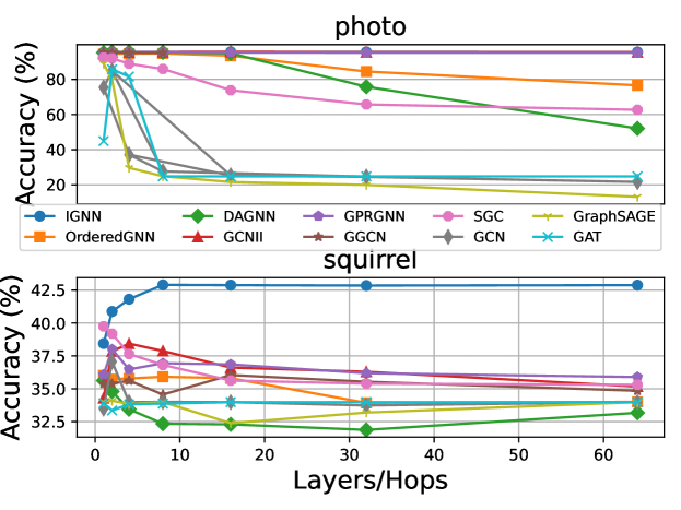
Figure 3. Performance of Different Neighborhood Range

6. Conclusion

In this paper, we propose a universal message-passing framework called Inceptive Graph Neural Network (IGNN). Through theoretical analysis, we reveal the limitations imposed by cascade dependency in multi-hop learning, which leads to a smoothness-generalization dilemma that hinders learning in both homophilic and heterophilic contexts. Our framework eliminates this dilemma by leveraging three key principles: separative neighborhood transformation, inceptive neighborhood aggregation, and neighborhood relationship learning. These principles enable the model to learn independent representations across multiple receptive hops. This approach enhances the ability of GNNs to adapt to varying levels of homophily across multiple hops, with personalized generalization capabilities for each hop, making IGNN a versatile solution.

Appendix A Appendix of Proofs

A.1. Proofs of Theorems 4.1 and Corollary 4.2

proof of Theorem 4.1.

To prove Theorem 4.1, we need to borrow the following notations and Lemmas from (Oono and Suzuki, 2019). For $N,D,F\in\mathbb{N}_{+}$, $\widehat{\mathbf{A}}\in\mathbb{R}^{N\times N}$ is a symmetric matrix and $\mathbf{W}^{(k)}\in\mathbb{R}^{D\times F}$ for $k\in\mathbb{N}_{+}$. For $M\leq N$, let $\mathbf{U}$ be a $M$-dimensional subspace of $\mathbb{R}^{N}$. We assume $\mathbf{U}$ and $\widehat{\mathbf{A}}$ satisfy the following properties that generalize the situation where $\mathbf{U}$ is the eigenspace associated with the smallest eigenvalue of the graph Laplacian $\widehat{\mathbf{L}}=\mathbf{I}_{N}-\widehat{\mathbf{A}}$ (that is, zero). We endow $\mathbb{R}^{N}$ with the ordinal inner product and denote the orthogonal complement of $\mathbf{U}$ by $\mathbf{U}^{\perp}:=\left\{\mathbf{u}\in\mathbb{R}^{N}\mid\langle\mathbf{u},\mathbf{v}\rangle=0,\forall\mathbf{v}\in\mathbf{U}\right\}$. We can regard $\widehat{\mathbf{A}}$ as a linear mapping $\left.\widehat{\mathbf{A}}\right|_{\mathbf{U}^{\perp}}:\mathbf{U}^{\perp}\rightarrow\mathbf{U}^{\perp}$. Choose the orthonormal basis $\left(e_{m}\right)_{m=M+1,\ldots,N}$ of $U^{\perp}$ consisting of the eigenvalue of $\left.\widehat{\mathbf{A}}\right|_{U^{\perp}}$. Let $\lambda_{m}$ be the eigenvalue of $\widehat{\mathbf{A}}$ to which $e_{m}$ is associated $(m=M+1,\ldots,N)$. Note that since the operator norm of $\left.\widehat{\mathbf{A}}\right|_{\mathbf{U}^{\perp}}$ is $\lambda$, we have $\left|\lambda_{m}\right|\leq\lambda$ for all $m=M+1,\ldots,N$. Since $\left(e_{m}\right)_{m\in[N]}$ forms the orthonormal basis of $\mathbb{R}^{N}$, we can uniquely write $\mathbf{X}\in\mathbb{R}^{N\times D}$ as $\mathbf{X}=\sum_{m=1}^{N}e_{m}\otimes\boldsymbol{\omega}_{m}$ for some $\boldsymbol{\omega}_{m}\in\mathbb{R}^{D}$ with $\otimes$ denoting the Kronecker product. Then, we have

(16) $$d_{\mathcal{M}}^{2}(\mathbf{X})=\sum_{m=M+1}^{N}\left\|\boldsymbol{\omega}_{m}\right\|_{2}^{2},$$

where $\|\cdot\|_{2}$ is the 2-norm. On the other hand, we have

(17) $$\begin{split}\widehat{\mathbf{A}}\mathbf{X}\mathbf{W}^{(k)}=&\sum_{m=1}^{N}(\widehat{\mathbf{A}}e_{m})\otimes({\mathbf{W}^{(k)}}^{\top}\boldsymbol{\omega}_{m})\\ =&\sum_{m=1}^{M}(\widehat{\mathbf{A}}e_{m})\otimes({\mathbf{W}^{(k)}}^{\top}\boldsymbol{\omega}_{m})+\sum_{m=M+1}^{N}(\widehat{\mathbf{A}}e_{m})\otimes({\mathbf{W}^{(k)}}^{\top}\boldsymbol{\omega}_{m})\\ =&\sum_{m=1}^{M}(\widehat{\mathbf{A}}e_{m})\otimes({\mathbf{W}^{(k)}}^{\top}\boldsymbol{\omega}_{m})+\sum_{m=M+1}^{N}e_{m}\otimes(\lambda_{m}{\mathbf{W}^{(k)}}^{\top}\boldsymbol{\omega}_{m}).\end{split}$$

Since $\mathbf{U}$ is invariant under $\widehat{\mathbf{A}}$ (Oono and Suzuki, 2019), for any $m\in[M]$, we can write $\widehat{\mathbf{A}}e_{m}$ as a linear combination of $e_{n}(n\in[M])$. Therefore, we have

(18) $$d_{\mathcal{M}}^{2}\left(\widehat{\mathbf{A}}\mathbf{X}\mathbf{W}^{(k)}\right)=\sum_{m=M+1}^{N}\left\|\lambda_{m}{\mathbf{W}^{(k)}}^{\top}\boldsymbol{\omega}_{m}\right\|^{2}_{2}.$$

Lemma A.1 (Oono and Suzuki (2019)).

For any $\mathbf{X}\in\mathbb{R}^{N\times D}$, we have $d_{\mathcal{M}}(\sigma(\mathbf{X}))\leq d_{\mathcal{M}}(\mathbf{X})$.

Based on Lemma A.1, we have

(19) $$\begin{split}d_{\mathcal{M}}^{2}\left(\mathbf{H}_{\widehat{\mathbf{A}}}^{(k)}\right)=&d_{\mathcal{M}}^{2}\left(\sigma(\widehat{\mathbf{A}}\mathbf{H}_{\widehat{\mathbf{A}}}^{(k-1)}\mathbf{W}^{(k)})\right)\\ \leqslant&d_{\mathcal{M}}^{2}\left(\widehat{\mathbf{A}}\sigma\left(\widehat{\mathbf{A}}\mathbf{H}_{\widehat{\mathbf{A}}}^{(k-2)}\mathbf{W}^{(k-1)}\right)\mathbf{W}^{(k)}\right)\\ \leqslant&d_{\mathcal{M}}^{2}\left(\widehat{\mathbf{A}}^{2}\mathbf{H}_{\widehat{\mathbf{A}}}^{(k-2)}\mathbf{W}^{(k-1)}\mathbf{W}^{(k)}\right)\\ \leqslant&d_{\mathcal{M}}^{2}\left(\widehat{\mathbf{A}}^{k}\mathbf{X}\mathbf{W}^{(1)}\mathbf{W}^{(2)}\ldots\mathbf{W}^{(k)}\right)\\ =&\sum_{m=M+1}^{N}\left\|\lambda_{m}^{k}\left(\mathbf{W}^{(1)}\ldots\mathbf{W}^{(k)}\right)^{\top}\boldsymbol{\omega}_{m}\right\|^{2}_{2}.\\ \end{split}$$

Lemma A.2 (Juvina et al. ([n. d.])).

For any $k$-layer GCN with 1-Lipschitz activation functions (e.g. ReLU, Leaky ReLU, SoftPlus, Tanh or Sigmoid), defined as $\mathbf{H}^{(k)}=\sigma(\widehat{\mathbf{A}}\mathbf{H}^{(k-1)}\mathbf{W}^{(k)})$, the Lipschitz constant becomes

(20) $$\hat{L}_{G}=\left\|\prod_{i=1}^{k}\mathbf{W}^{(i)}\right\|_{2}.$$

We recall the the Lipschitz constant $\hat{L}_{G}$ of GCN (Juvina et al., [n. d.]) as in Lemma A.2, and substitute (20) into (19), we have:

(21) $$\begin{split}d_{\mathcal{M}}^{2}\left(\mathbf{H}_{\widehat{\mathbf{A}}}^{(k)}\right)\leqslant&\sum_{m=M+1}^{N}\left\|\lambda_{m}^{k}\left(\mathbf{W}^{(1)}\ldots\mathbf{W}^{(k)}\right)^{\top}\boldsymbol{\omega}_{m}\right\|^{2}_{2}\\ \leqslant&\sum_{m=M+1}^{N}\lambda_{m}^{2k}\|\boldsymbol{\omega}_{m}\|_{2}^{2}\left\|\prod_{i=1}^{k}\mathbf{W}^{(i)}\right\|_{2}^{2}\\ =&\hat{L}_{G}^{2}\sum_{m=M+1}^{N}\lambda_{m}^{2k}\|\boldsymbol{\omega}_{m}\|_{2}^{2}\\ \leqslant&\hat{L}_{G}^{2}\lambda^{2k}\sum_{m=M+1}^{N}\|\boldsymbol{\omega}_{m}\|_{2}^{2}\quad\quad=\hat{L}_{G}^{2}\lambda^{2k}d_{\mathcal{M}}^{2}(\mathbf{X}).\end{split}$$

∎

proof of Corollary 4.2.

In order to have $d_{\mathcal{M}}(\mathbf{H}_{\widehat{\mathbf{A}}}^{(k)})\leq\hat{L}_{G}\lambda^{k}\mathcal{D}<\epsilon$, since $\hat{L}_{G}>=0$, $\mathcal{D}>=0$ and $\lambda<1$, we have

(22) $$\begin{split}d_{\mathcal{M}}(\mathbf{H}_{\widehat{\mathbf{A}}}^{(k)})\leq\hat{L}_{G}\lambda^{k}\mathcal{D}<\epsilon\Rightarrow\lambda^{k}&<\frac{\epsilon}{\hat{L}_{G}\mathcal{D}},\\ \Rightarrow k\log\lambda&<\log\frac{\epsilon}{\hat{L}_{G}\mathcal{D}},\\ \Rightarrow k&>\frac{\log\frac{\epsilon}{\hat{L}_{G}\mathcal{D}}}{\log\lambda}.\end{split}$$

Therefore, there exists $k^{*}=\lceil{\frac{\log\frac{\epsilon}{\hat{L}_{G}\mathcal{D}}}{\log\lambda}}\rceil$, such that $d_{\mathcal{M}}(\mathbf{H}_{\widehat{\mathbf{A}}}^{(k^{*})})\leq\hat{L}_{G}\lambda^{(}k^{*})\mathcal{D}<\epsilon$, where $\lceil{\cdot}\rceil$ is the ceil of the input. ∎

Proof of Theorem 4.3.

(23) $$d_{\mathcal{M}}^{2}(\mathbf{H}_{IG,k}) =d_{\mathcal{M}}^{2}\left(\sigma\left((\|_{i=0}^{k}\sigma(\widehat{\mathbf{A}}^{i}\mathbf{X}\mathbf{W}^{(i)}))\mathbf{W}\right)\right)$$

$$=d_{\mathcal{M}}^{2}\left(\sigma\left(\sum_{i=0}^{k}\sigma(\widehat{\mathbf{A}}^{i}\mathbf{X}\mathbf{W}^{(i)})\mathbf{W}_{i}\right)\right)$$

$$\leqslant d_{\mathcal{M}}^{2}\left(\sum_{i=0}^{k}\widehat{\mathbf{A}}^{i}\mathbf{X}\mathbf{W}^{(i)}\mathbf{W}_{i}\right),\mathbf{W}=\left[\begin{smallmatrix}\mathbf{W}_{0}\\ \cdots\\ \mathbf{W}_{i}\\ \cdots\\ \mathbf{W}_{k}\end{smallmatrix}\right].$$

Given $\mathbf{U}$ invariant under $\widehat{\mathbf{A}}$, $\mathbf{U}$ is also invariant under $\widehat{\mathbf{A}}^{i}$. Similar to the derivation of Equation (18), we have

(24) $$d_{\mathcal{M}}^{2}(\mathbf{H}_{IG,k}) \leqslant d_{\mathcal{M}}^{2}\left(\sum_{i=0}^{k}\widehat{\mathbf{A}}^{i}\mathbf{X}\mathbf{W}^{(i)}\mathbf{W}_{i}\right)$$

$$=\sum_{m=M+1}^{N}\left\|\sum_{i=0}^{k}\lambda_{m}^{i}(\mathbf{W}^{(i)}\mathbf{W}_{i})^{\top}\boldsymbol{\omega}_{m}\right\|_{2}^{2}$$

$$\leqslant\sum_{m=M+1}^{N}\left\|\sum_{i=0}^{k}\lambda^{i}(\mathbf{W}^{(i)}\mathbf{W}_{i})^{\top}\boldsymbol{\omega}_{m}\right\|_{2}^{2}$$

$$\leqslant\sum_{m=M+1}^{N}\|\boldsymbol{\omega}_{m}\|_{2}^{2}\left\|\sum_{i=0}^{k}\lambda^{i}\mathbf{W}^{(i)}\mathbf{W}_{i}\right\|_{2}^{2}$$

$$=\left\|\sum_{i=0}^{k}\lambda^{i}\mathbf{W}^{(i)}\mathbf{W}_{i}\right\|_{2}^{2}\sum_{m=M+1}^{N}\|\boldsymbol{\omega}_{m}\|_{2}^{2}$$

$$=\left\|\sum_{i=0}^{k}\lambda^{i}\mathbf{W}^{(i)}\mathbf{W}_{i}\right\|_{2}^{2}d_{\mathcal{M}}^{2}(\mathbf{X})$$

$$=\left\|\sum_{i=0}^{k}\lambda^{i}\mathbf{W}^{(i)}\mathbf{W}_{i}\right\|_{2}^{2}\mathcal{D}^{2}.$$

Recall the Theorem 3.1 in Khromov and Singh (2024) as following Theorem A.3. Similar to Equation (23), we can obtain $\mathbf{H}_{IG,k}=\sigma(\sum_{i=0}^{k}\sigma(\widehat{\mathbf{A}}^{i}\mathbf{X}\mathbf{W}^{(i)})\mathbf{W}_{i})$. Since $\lambda_{K}=1$ for $\widehat{\mathbf{A}}^{i}$, applying Theorem A.3 to IGNN, we have

(25) $$\hat{L}_{IG}=\varphi\left(1\right)=\|\sum_{i=0}^{k}\mathbf{W}^{(i)}\mathbf{W}_{i}\|.$$

Theorem A.3 (Juvina et al. ([n. d.])).

Consider a generic graph convolutional neural network like $\mathbf{H}^{(k)}=\sigma(\mathbf{H}^{(k-1)}\mathbf{W}_{0}^{(k)}+\mathbf{M}\mathbf{H}^{(k-1)}\mathbf{W}_{1}^{(k)})$ with $\mathbf{M}$ symmetric (corresponding to an undirected graph) with non-negative elements. Let $\lambda_{K}\geq 0$ be its maximum eigenvalue. Assume that, for every $i\in\{1,\ldots,k\}$, matrices $\mathbf{W}_{0}^{(i)}$ and $\mathbf{W}_{1}^{(i)}$ have non-negative elements, $\mathbf{W}_{0}^{(i)}\geq 0$ and $\mathbf{W}_{1}^{(i)}\geq 0$. Let

(26) $$(\forall\mu\in\mathbb{R})\quad\varphi(\mu)=\left\|\left(\mathbf{W}_{0}^{(k)}+\mu\mathbf{W}_{1}^{(k)}\right)\cdots\left(\mathbf{W}_{0}^{(1)}+\mu\mathbf{W}_{1}^{(1)}\right)\right\|_{\mathrm{s}}.$$

Then, a Lipschitz constant of the network is given by

(27) $$\hat{L}=\varphi\left(\lambda_{K}\right).$$

∎

A.2. Proof of Theorem 4.4

Proof of Theorem 4.4.

A polynomial graph filter (Defferrard et al., 2016) on $\widehat{\mathbf{A}}$ is defined as:

(28) $$\begin{split}\mathbf{H}_{p}&=\left(\sum_{k=0}^{K}\theta_{k}\widehat{\mathbf{L}}^{k}\right)\mathbf{X}=\left(\sum_{k=0}^{K}\theta_{k}(\mathbf{I}_{N}-\widehat{\mathbf{A}})^{k}\right)\mathbf{X}.\end{split}$$

Expanding the expression $(\mathbf{I}_{N}-\widehat{\mathbf{A}})^{k}$ using the binomial theorem and changing the order of summation, we have:

(29) $$\begin{split}\mathbf{H}_{p}&=\left(\sum_{k=0}^{K}\theta_{k}\left(\sum_{i=0}^{k}(-1)^{i}{k\choose i}\widehat{\mathbf{A}}^{i}\right)\right)\mathbf{X}=\left(\sum_{i=0}^{K}\left(\sum_{k=i}^{K}\theta_{k}(-1)^{i}{k\choose i}\widehat{\mathbf{A}}^{i}\right)\right)\mathbf{X}.\end{split}$$

Meanwhile, IGNN in (LABEL:eq:_hop-wise_relation_matrix) can be written as:

(30) $$\mathbf{H}=\sigma\left((\underset{k=0}{\overset{K}{||}}\sigma(\widehat{\mathbf{A}}^{k}\mathbf{X}\mathbf{W}^{(k)}))\mathbf{W}\right)=\sigma\left(\sum_{k=0}^{K}\sigma(\widehat{\mathbf{A}}^{k}\mathbf{X}\mathbf{W}^{(k)})\mathbf{W}_{k}\right),$$

where $\mathbf{W}=\left[\begin{smallmatrix}\mathbf{W}_{0}\\ \cdots\\ \mathbf{W}_{k}\\ \cdots\\ \mathbf{W}_{K}\end{smallmatrix}\right]$. Simplifying (30) by leaving out all the non-linear layers and setting $\mathbf{W}^{(k)}=\mathbf{I}$, $\mathbf{W}_{k}=(\sum_{i=k}^{K}\theta_{i}(-1)^{k}{i\choose k})\mathbf{I}$, we have:

(31) $$\mathbf{H}=\sum_{k=0}^{K}(\widehat{\mathbf{A}}^{k}\mathbf{X}\mathbf{I})(\sum_{i=k}^{K}\theta_{i}(-1)^{k}{i\choose k})\mathbf{I}=\sum_{k=0}^{K}\sum_{i=k}^{K}\theta_{i}(-1)^{k}{i\choose k}\widehat{\mathbf{A}}^{k}\mathbf{X}.$$

Swap the notation of $i$ and $k$, we get $\mathbf{H}=\sum_{i=0}^{K}\sum_{k=i}^{K}\theta_{k}(-1)^{i}{k\choose i}\widehat{\mathbf{A}}^{i}\mathbf{X}$, which is the same as the polynomial graph filter in (28).

∎

Table 6. Comparison of Inceptive GNNs in incorporating three principles.

Methods	APPNP	JKNet-GCN	IncepGCN	SIGN	MIXHOP	DAGNN	GCNII	GPRGCNN	ACMGCN	OrderedGNN	IGNN
SN			✓	✓	✓						✓
IN	✓	✓	✓	✓	✓	✓	✓	✓	✓	✓	✓
NR		✓				✓		✓	✓	✓	✓

A.3. Proofs of Propositions 4.5 and 4.6

Proof 1: SIGN as a simplified case of IGNN.

The architecture of SIGN can be trivially obtained by omitting the NR function and replacing it with a non-learnable concatenation as

(32) $$\mathbf{H}=\underset{k=0}{\overset{K}{||}}\sigma(\widehat{\mathbf{A}}^{k}\mathbf{X}\mathbf{W}^{(k)}).$$

∎

Proof 2: APPNP as a simplified case of IGNN.

The architecture of APPNP (Gasteiger et al., 2018) is defined as follows:

(33) $$\begin{split}\mathbf{H}^{(0)}_{\text{APPNP}}=f_{\theta}(\mathbf{X})=\mathbf{X}\mathbf{W}_{\theta},\mathbf{H}^{(k)}_{\text{APPNP}}=(1-\alpha)\widehat{\mathbf{A}}\mathbf{H}^{(k-1)}_{\text{APPNP}}+\alpha\mathbf{H}^{(0)}_{\text{APPNP}},\end{split}$$

where $\alpha\in(0,1]$ represents the teleport (or restart) probability. Consequently, $\mathbf{H}^{(k)}_{\text{APPNP}}$ can be expressed in terms of $\mathbf{H}^{(0)}_{\text{APPNP}}$ as:

(34) $$\mathbf{H}^{(k)}_{\text{APPNP}}=(1-\alpha)^{k}\widehat{\mathbf{A}}^{k}\mathbf{H}^{(0)}_{\text{APPNP}}+\sum_{i=0}^{k-1}\alpha(1-\alpha)^{i}\widehat{\mathbf{A}}^{i}\mathbf{H}^{(0)}_{\text{APPNP}}.$$

According to (30), by omitting all non-linearity and setting $\mathbf{W}^{(k)}=\mathbf{W}_{\theta}$, $\mathbf{W}_{K}=(1-\alpha)^{K}\mathbf{I}$, and $\mathbf{W}_{k}=\alpha(1-\alpha)^{k}\mathbf{I}$ for $k\in[0,K-1]$, we obtain a simplified case of IGNN as:

(35) $$\begin{split}\mathbf{H}&=\widehat{\mathbf{A}}^{K}\mathbf{X}\mathbf{W}_{\theta}(1-\alpha)^{K}\mathbf{I}+\sum_{k=0}^{K-1}\widehat{\mathbf{A}}^{k}\mathbf{X}\mathbf{W}_{\theta}\alpha(1-\alpha)^{k}\mathbf{I}\\ &=(1-\alpha)^{K}\widehat{\mathbf{A}}^{K}\mathbf{X}\mathbf{W}_{\theta}+\sum_{k=0}^{K-1}\alpha(1-\alpha)^{k}\widehat{\mathbf{A}}^{k}\mathbf{X}\mathbf{W}_{\theta}\\ &=\mathbf{H}^{(K)}_{\text{APPNP}}.\end{split}$$

∎

Proof 3: MixHop as a simplified case of IGNN.

Here, we illustrate that hop-wise neighborhood relationships can achieve the general layer-wise neighborhood mixing of MixHop Abu-El-Haija et al. (2019) by specializing the weight matrix as $\mathbf{W}=\left[\begin{smallmatrix}\mathbf{W}_{0}\\ \cdots\\ \mathbf{W}_{k}\\ \cdots\\ \mathbf{W}_{K}\end{smallmatrix}\right]\in\mathbb{R}^{KF\times F^{\prime}}$:

(36) $$\begin{split}\mathbf{H}&=\sigma\left((\underset{k=0}{\overset{K}{||}}\sigma(\widehat{\mathbf{A}}^{k}\mathbf{X}\mathbf{W}^{(k)}))\mathbf{W}\right)=\sigma\left(\sum_{k=0}^{K}\sigma(\widehat{\mathbf{A}}^{k}\mathbf{X}\mathbf{W}^{(k)})\mathbf{W}_{k}\right),\end{split}$$

where $\ \mathbf{W}^{(k)}\in\mathbb{R}^{D\times F}$, $\mathbf{W}_{k}\in\mathbb{R}^{F\times F^{\prime}}$. Setting $F^{\prime}=F=D$, $\mathbf{W}^{(k)}=\mathbf{I}_{F}$ and $\mathbf{W}_{k}=\alpha_{k}\mathbf{I}_{F}$ results in:

(37) $$\begin{split}\mathbf{h}_{v}&=\sigma\left(\sum_{k=0}^{K}\sigma(\widehat{\mathbf{A}}^{k}\mathbf{X}\mathbf{W}^{(k)})(\alpha_{k}\mathbf{I}_{F})\right)=\sigma\left(\sum_{k=0}^{K}\alpha_{k}\sigma(\widehat{\mathbf{A}}^{k}\mathbf{X}\mathbf{W}^{(k)})\right)\\ &=\sigma\left(\sum_{k=0}^{K}\alpha_{k}\sigma(\widehat{\mathbf{A}}^{k}\mathbf{X})\right),\end{split}$$

which represents a general layer-wise neighborhood mixing relationship demonstrated by Definition 2 of  Abu-El-Haija et al. (2019) to exceed the representational capacity of vanilla GCNs within the traditional message-passing framework. We achieve this advantage through simple neighborhood concatenation and non-linear feature transformation, eliminating the need to stack multiple layers of message passing as done in Abu-El-Haija et al. (2019), thus calling it Hop-wise Neighborhood Relation rather than layer-wise. ∎

Proof 4: GPRGNN as a simplified case of IGNN.

Based on (36), by sharing the parameters of all $\mathbf{W}^{(k)}$ as $\mathbf{W}^{(k)}=\mathbf{W}_{\theta}$, setting $\mathbf{W}_{k}=\gamma_{k}\mathbf{I}$ and leaving out all the non-linear layers of $\text{{REL}}(\cdot)$, we have:

(38) $$\mathbf{H}=\sum_{k=0}^{K}(\widehat{\mathbf{A}}^{k}\mathbf{X}\mathbf{W}^{(k)})\mathbf{W}_{k}=\sum_{k=0}^{K}(\widehat{\mathbf{A}}^{k}\mathbf{X}\mathbf{W}_{\theta})\gamma_{k}\mathbf{I}=\sum_{k=0}^{K}\gamma_{k}(\widehat{\mathbf{A}}^{k}\mathbf{X}\mathbf{W}_{\theta}),$$

which is the exact architecture of GPRGNN (Chien et al., 2020). ∎

Proof 5: mean/sum pooling as a simplified case of IGNN.

Based on (36), by setting $\mathbf{W}_{k}=\frac{1}{K}\mathbf{I}$, we obtain $\mathbf{H}=\sigma\left(\sum_{k=0}^{K}\frac{1}{K}\sigma(\widehat{\mathbf{A}}^{k}\mathbf{X}\mathbf{W}^{(k)})\right)$, which corresponds to mean pooling. Alternatively, by setting $\mathbf{W}_{k}=\mathbf{I}$, we have $\mathbf{H}=\sigma\left(\sum_{k=0}^{K}\sigma(\widehat{\mathbf{A}}^{k}\mathbf{X}\mathbf{W}^{(k)})\right)$, which corresponds to sum pooling. ∎

Appendix B Appendix of Additional Results

B.1. Comparision of Inceptive GNNs

Table 6 shows the comparison of inceptive GNNs in incorporating three principles. Except for IGNN, the other methods lack at least one principle. The best porformance of IGNN shows that the combination of all three principles can best eliminate the dilemma.

References

- (1)
- Abu-El-Haija et al. (2019) Sami Abu-El-Haija, Bryan Perozzi, Amol Kapoor, Nazanin Alipourfard, Kristina Lerman, Hrayr Harutyunyan, Greg Ver Steeg, and Aram Galstyan. 2019. Mixhop: Higher-order graph convolutional architectures via sparsified neighborhood mixing. In international conference on machine learning. PMLR, 21–29.
- Ai et al. (2024) Guoguo Ai, Hui Yan, Huan Wang, and Xin Li. 2024. A2GCN: Graph Convolutional Networks with Adaptive Frequency and Arbitrary Order. Pattern Recognition 156 (2024), 110764.
- Bo et al. (2021) Deyu Bo, Xiao Wang, Chuan Shi, and Huawei Shen. 2021. Beyond low-frequency information in graph convolutional networks. In Proceedings of the AAAI conference on artificial intelligence, Vol. 35. 3950–3957.
- Chen et al. (2020) Ming Chen, Zhewei Wei, Zengfeng Huang, Bolin Ding, and Yaliang Li. 2020. Simple and deep graph convolutional networks. In International conference on machine learning. PMLR, 1725–1735.
- Chien et al. (2020) Eli Chien, Jianhao Peng, Pan Li, and Olgica Milenkovic. 2020. Adaptive universal generalized pagerank graph neural network. arXiv preprint arXiv:2006.07988 (2020).
- Defferrard et al. (2016) Michaël Defferrard, Xavier Bresson, and Pierre Vandergheynst. 2016. Convolutional neural networks on graphs with fast localized spectral filtering. Advances in neural information processing systems 29 (2016).
- Du et al. (2022) Lun Du, Xiaozhou Shi, Qiang Fu, Xiaojun Ma, Hengyu Liu, Shi Han, and Dongmei Zhang. 2022. Gbk-gnn: Gated bi-kernel graph neural networks for modeling both homophily and heterophily. In Proceedings of the ACM Web Conference 2022. 1550–1558.
- Fan et al. (2019) Wenqi Fan, Yao Ma, Qing Li, Yuan He, Eric Zhao, Jiliang Tang, and Dawei Yin. 2019. Graph neural networks for social recommendation. In The world wide web conference. 417–426.
- Frasca et al. (2020) Fabrizio Frasca, Emanuele Rossi, Davide Eynard, Ben Chamberlain, Michael Bronstein, and Federico Monti. 2020. Sign: Scalable inception graph neural networks. arXiv preprint arXiv:2004.11198 (2020).
- Gasteiger et al. (2018) Johannes Gasteiger, Aleksandar Bojchevski, and Stephan Günnemann. 2018. Predict then propagate: Graph neural networks meet personalized pagerank. arXiv preprint arXiv:1810.05997 (2018).
- Gilmer et al. (2017) Justin Gilmer, Samuel S Schoenholz, Patrick F Riley, Oriol Vinyals, and George E Dahl. 2017. Neural message passing for quantum chemistry. In International conference on machine learning. PMLR, 1263–1272.
- Hamilton et al. (2017) Will Hamilton, Zhitao Ying, and Jure Leskovec. 2017. Inductive representation learning on large graphs. Advances in neural information processing systems 30 (2017).
- He et al. (2016) Kaiming He, Xiangyu Zhang, Shaoqing Ren, and Jian Sun. 2016. Deep residual learning for image recognition. In Proceedings of the IEEE conference on computer vision and pattern recognition. 770–778.
- Juvina et al. ([n. d.]) Simona Ioana Juvina, Ana Antonia Neacșu, Jérôme Rony, Jean-Christophe Pesquet, Corneliu Burileanu, and Ismail Ben Ayed. [n. d.]. Training Graph Neural Networks Subject to a Tight Lipschitz Constraint. Transactions on Machine Learning Research ([n. d.]).
- Khromov and Singh (2024) Grigory Khromov and Sidak Pal Singh. 2024. Some Fundamental Aspects about Lipschitz Continuity of Neural Networks. In The Twelfth International Conference on Learning Representations.
- Kingma Diederik and Adam (2014) P Kingma Diederik and Jimmy Ba Adam. 2014. A method for stochastic optimization. arXiv preprint arXiv:1412.6980 (2014).
- Kipf and Welling (2016) Thomas N Kipf and Max Welling. 2016. Semi-supervised classification with graph convolutional networks. arXiv preprint arXiv:1609.02907 (2016).
- Li et al. (2022) Xiang Li, Renyu Zhu, Yao Cheng, Caihua Shan, Siqiang Luo, Dongsheng Li, and Weining Qian. 2022. Finding global homophily in graph neural networks when meeting heterophily. In International Conference on Machine Learning. PMLR, 13242–13256.
- Liu et al. (2021) GuanJun Liu, Jing Tang, Yue Tian, and Jiacun Wang. 2021. Graph neural network for credit card fraud detection. In 2021 International Conference on Cyber-Physical Social Intelligence (ICCSI). IEEE, 1–6.
- Liu et al. (2024) Meihan Liu, Zeyu Fang, Zhen Zhang, Ming Gu, Sheng Zhou, Xin Wang, and Jiajun Bu. 2024. Rethinking propagation for unsupervised graph domain adaptation. In Proceedings of the AAAI Conference on Artificial Intelligence, Vol. 38. 13963–13971.
- Liu et al. (2020) Meng Liu, Hongyang Gao, and Shuiwang Ji. 2020. Towards deeper graph neural networks. In Proceedings of the 26th ACM SIGKDD international conference on knowledge discovery & data mining. 338–348.
- Luan et al. (2024) Sitao Luan, Chenqing Hua, Qincheng Lu, Liheng Ma, Lirong Wu, Xinyu Wang, Minkai Xu, Xiao-Wen Chang, Doina Precup, Rex Ying, et al. 2024. The Heterophilic Graph Learning Handbook: Benchmarks, Models, Theoretical Analysis, Applications and Challenges. arXiv preprint arXiv:2407.09618 (2024).
- Luan et al. (2022) Sitao Luan, Chenqing Hua, Qincheng Lu, Jiaqi Zhu, Mingde Zhao, Shuyuan Zhang, Xiao-Wen Chang, and Doina Precup. 2022. Revisiting heterophily for graph neural networks. Advances in neural information processing systems 35 (2022), 1362–1375.
- Ma et al. (2022) Yao Ma, Xiaorui Liu, Neil Shah, and Jiliang Tang. 2022. IS HOMOPHILY A NECESSITY FOR GRAPH NEURAL NETWORKS?. In 10th International Conference on Learning Representations, ICLR 2022.
- Ma et al. (2021) Yao Ma, Xiaorui Liu, Tong Zhao, Yozen Liu, Jiliang Tang, and Neil Shah. 2021. A unified view on graph neural networks as graph signal denoising. In Proceedings of the 30th ACM International Conference on Information & Knowledge Management. 1202–1211.
- Mao et al. (2024) Haitao Mao, Zhikai Chen, Wei Jin, Haoyu Han, Yao Ma, Tong Zhao, Neil Shah, and Jiliang Tang. 2024. Demystifying structural disparity in graph neural networks: Can one size fit all? Advances in neural information processing systems 36 (2024).
- Oono and Suzuki (2019) Kenta Oono and Taiji Suzuki. 2019. On asymptotic behaviors of graph cnns from dynamical systems perspective. arXiv preprint arXiv:1905.10947 (2019).
- Pan and Kang (2023) Erlin Pan and Zhao Kang. 2023. Beyond homophily: Reconstructing structure for graph-agnostic clustering. In International Conference on Machine Learning. PMLR, 26868–26877.
- Pei et al. (2020) Hongbin Pei, Bingzhe Wei, Kevin Chen-Chuan Chang, Yu Lei, and Bo Yang. 2020. Geom-gcn: Geometric graph convolutional networks. arXiv preprint arXiv:2002.05287 (2020).
- Rong et al. (2019) Yu Rong, Wenbing Huang, Tingyang Xu, and Junzhou Huang. 2019. Dropedge: Towards deep graph convolutional networks on node classification. arXiv preprint arXiv:1907.10903 (2019).
- Scarselli et al. (2008) Franco Scarselli, Marco Gori, Ah Chung Tsoi, Markus Hagenbuchner, and Gabriele Monfardini. 2008. The graph neural network model. IEEE transactions on neural networks 20, 1 (2008), 61–80.
- Shuman et al. (2013) David I Shuman, Sunil K Narang, Pascal Frossard, Antonio Ortega, and Pierre Vandergheynst. 2013. The emerging field of signal processing on graphs: Extending high-dimensional data analysis to networks and other irregular domains. IEEE signal processing magazine 30, 3 (2013), 83–98.
- Song et al. (2023) Yunchong Song, Chenghu Zhou, Xinbing Wang, and Zhouhan Lin. 2023. Ordered GNN: Ordering Message Passing to Deal with Heterophily and Over-smoothing. In The Eleventh International Conference on Learning Representations. https://openreview.net/forum?id=wKPmPBHSnT6
- Szegedy (2013) C Szegedy. 2013. Intriguing properties of neural networks. arXiv preprint arXiv:1312.6199 (2013).
- Szegedy et al. (2015) Christian Szegedy, Wei Liu, Yangqing Jia, Pierre Sermanet, Scott Reed, Dragomir Anguelov, Dumitru Erhan, Vincent Vanhoucke, and Andrew Rabinovich. 2015. Going deeper with convolutions. In Proceedings of the IEEE conference on computer vision and pattern recognition. 1–9.
- Tang and Liu (2023) Huayi Tang and Yong Liu. 2023. Towards understanding generalization of graph neural networks. In International Conference on Machine Learning. PMLR, 33674–33719.
- Velickovic et al. (2017) Petar Velickovic, Guillem Cucurull, Arantxa Casanova, Adriana Romero, Pietro Lio, Yoshua Bengio, et al. 2017. Graph attention networks. stat 1050, 20 (2017), 10–48550.
- Virmaux and Scaman (2018) Aladin Virmaux and Kevin Scaman. 2018. Lipschitz regularity of deep neural networks: analysis and efficient estimation. Advances in Neural Information Processing Systems 31 (2018).
- Wang et al. (2022) Tao Wang, Di Jin, Rui Wang, Dongxiao He, and Yuxiao Huang. 2022. Powerful graph convolutional networks with adaptive propagation mechanism for homophily and heterophily. In Proceedings of the AAAI conference on artificial intelligence, Vol. 36. 4210–4218.
- Wu et al. (2019) Felix Wu, Amauri Souza, Tianyi Zhang, Christopher Fifty, Tao Yu, and Kilian Weinberger. 2019. Simplifying graph convolutional networks. In International conference on machine learning. PMLR, 6861–6871.
- Wu et al. (2023a) Qitian Wu, Chenxiao Yang, Wentao Zhao, Yixuan He, David Wipf, and Junchi Yan. 2023a. DIFFormer: Scalable (Graph) Transformers Induced by Energy Constrained Diffusion. In International Conference on Learning Representations (ICLR).
- Wu et al. (2022) Qitian Wu, Wentao Zhao, Zenan Li, David Wipf, and Junchi Yan. 2022. NodeFormer: A Scalable Graph Structure Learning Transformer for Node Classification. In Advances in Neural Information Processing Systems (NeurIPS).
- Wu et al. (2023b) Qitian Wu, Wentao Zhao, Chenxiao Yang, Hengrui Zhang, Fan Nie, Haitian Jiang, Yatao Bian, and Junchi Yan. 2023b. SGFormer: Simplifying and Empowering Transformers for Large-Graph Representations. In Advances in Neural Information Processing Systems (NeurIPS).
- Xu et al. (2018a) Keyulu Xu, Weihua Hu, Jure Leskovec, and Stefanie Jegelka. 2018a. How powerful are graph neural networks? arXiv preprint arXiv:1810.00826 (2018).
- Xu et al. (2018b) Keyulu Xu, Chengtao Li, Yonglong Tian, Tomohiro Sonobe, Ken-ichi Kawarabayashi, and Stefanie Jegelka. 2018b. Representation learning on graphs with jumping knowledge networks. In International conference on machine learning. PMLR, 5453–5462.
- Yan et al. (2022) Yujun Yan, Milad Hashemi, Kevin Swersky, Yaoqing Yang, and Danai Koutra. 2022. Two sides of the same coin: Heterophily and oversmoothing in graph convolutional neural networks. In 2022 IEEE International Conference on Data Mining (ICDM). IEEE, 1287–1292.
- Yang et al. (2022) Chenxiao Yang, Qitian Wu, Jiahua Wang, and Junchi Yan. 2022. Graph neural networks are inherently good generalizers: Insights by bridging gnns and mlps. arXiv preprint arXiv:2212.09034 (2022).
- Zaheer et al. (2017) Manzil Zaheer, Satwik Kottur, Siamak Ravanbakhsh, Barnabas Poczos, Russ R Salakhutdinov, and Alexander J Smola. 2017. Deep sets. Advances in neural information processing systems 30 (2017).
- Zheng et al. (2024) Zhuonan Zheng, Yuanchen Bei, Sheng Zhou, Yao Ma, Ming Gu, Hongjia Xu, Chengyu Lai, Jiawei Chen, and Jiajun Bu. 2024. Revisiting the Message Passing in Heterophilous Graph Neural Networks. arXiv preprint arXiv:2405.17768 (2024).
- Zhu et al. (2020) Jiong Zhu, Yujun Yan, Lingxiao Zhao, Mark Heimann, Leman Akoglu, and Danai Koutra. 2020. Beyond homophily in graph neural networks: Current limitations and effective designs. Advances in neural information processing systems 33 (2020), 7793–7804.
- Zhu et al. (2021) Meiqi Zhu, Xiao Wang, Chuan Shi, Houye Ji, and Peng Cui. 2021. Interpreting and unifying graph neural networks with an optimization framework. In Proceedings of the Web Conference 2021. 1215–1226.