Universality of extreme events in turbulent flows
Abstract
The universality of small scales, a cornerstone of turbulence, has been nominally confirmed for low-order mean-field statistics, such as the energy spectrum. However, small scales exhibit strong intermittency, exemplified by formation of extreme events which deviate anomalously from a mean-field description. Here, we investigate the universality of small scales by analyzing extreme events of velocity gradients in different turbulent flows, viz. direct numerical simulations (DNS) of homogeneous isotropic turbulence, inhomogeneous channel flow, and laboratory measurements in a von Karman mixing tank. We demonstrate that the scaling exponents of velocity gradient moments, as function of Reynolds number (), are universal, in agreement with previous studies at lower , and further show that even proportionality constants are universal when considering one moment order as a function of another. Additionally, by comparing various unconditional and conditional statistics across different flows, we demonstrate that the structure of the velocity gradient tensor is also universal. Overall, our findings provide compelling evidence that even extreme events are universal, with profound implications for turbulence theory and modeling.
In turbulent flows, energy is injected at large scales, and cascades across a wide range of intermediate scales down to very small scales, where it is dissipated into heat. The dynamics at large-scales depend on the geometry and specifics of the flow considered, rendering them inherently anisotropic and non-universal. However, as energy cascades to smaller scales, the influence of large-scales diminishes, leading to small scales becoming increasingly isotropic and universal. This notion underpins the foundational principle of small-scale universality, first proposed by Kolmogorov (1941) [1]—henceforth K41—which is a cornerstone of turbulence theory and modeling. It asserts that when the scale separation is sufficiently large (or equivalently the flow Reynolds number is large), the statistical properties of the small scales exhibit universal behavior, consistent across different turbulent flows. K41 further hypothesizes that the small scales are solely characterized by the fluid viscosity and the mean dissipation rate , which captures the net transfer of energy across the scales.
The most compelling support for small-scale universality comes from the well-known scaling of the energy spectrum in the inertial range (where viscosity can be neglected) and other similar results [2, 3]. In addition, studies have also investigated validity of local isotropy in the inertial range and also for velocity gradients [4, 5, 3, 6]. However, while K41 has been generally successful in describing low-order statistics, it is well-known that energy transfers in turbulence are highly intermittent, with fluctuations of dissipation rate, and velocity gradients in general, exhibiting large deviations from the mean [7, 8, 9, 10]. This phenomenon of intermittency, invalidates K41’s mean-field description [11, 12], and raises a natural question about the universality of extreme events, which is the motivation for this Letter.
Despite its obvious importance, the universality of extreme events has received limited attention. This gap arises primarily from challenges associated with measuring the full velocity gradient tensor in experiments [13]. Similarly, direct numerical simulations (DNS) were historically limited to lower due to their high computational cost [14]; with the constraints being even more severe for resolving extreme events [15, 16, 17, 10]. Nevertheless, DNS studies at low by [18, 19] have provided some support for universality by demonstrating identical scaling exponents of moments of dissipation-rate as function of . However, this only addresses part of the question and does not fully capture the structural complexity of velocity gradient tensor, which encompasses various non-trivial correlations between strain-rate and vorticity [20, 21, 22].
In this Letter, we address the universality of extreme events of velocity gradients, by examining turbulence in three distinct flows: DNS of homogeneous isotropic turbulence (HIT), DNS of plane channel flow, and laboratory experiments in a von Kármán mixing tank. These flows are all governed by the incompressible Navier-Stokes equations, differing only in large-scale geometry and forcing mechanisms. The DNS data utilized are at substantially higher than earlier studies, with the HIT runs corresponding to unprecedented small-scale resolution [23, 24]. Concurrently, the experimental data provides knowledge of the full velocity gradient tensor [25], providing structural information on extreme events which was not available previously.
By analyzing various statistics and the structure of the gradient tensor: (), we provide strong evidence in support of universality of extreme events. First, by considering velocity gradients moments, we show that their scaling exponents in are same in different flows, which substantially extends the results of [18] to higher and broader range of flow configurations. We then further show that even the proportionality constants can be matched across different flows, by considering one moment-order as a function of another, akin to extended self-similarity [26]. Beyond statistical moments, we also show that structural properties of extreme events, as captured by various conditional statistics, are quantitatively same across different flows, including their -dependence.
Data:
We only briefly describe the data used here since the three flows considered have been well studied on their own (though some additional details are also given in the Appendix A). We utilize the Taylor-scale Reynolds number for each flow, with being the rms of velocity fluctuations, and the Taylor length scale, where is the rms of longitudinal (diagonal) components of . Note that [11]. For HIT, the DNS data corresponds to several recent works [21, 23, 27, 28, 29, 30, 31], with the Taylor scale Reynolds number going from to , on grids of up to points. For channel flow, we utilize the Johns Hopkins turbulent database [32], with the skin-friction Reynolds numbers and . The experimental data corresponds to that of [25], with . While HIT is necessarily isotropic, it should be noted that plane channel flow is strongly anisotropic near the wall. In fact, it is known that the presence of a mean-shear persistently violates local isotropy [33, 34]. Consequently, for channel flow, statistics are obtained only in the outer region, in a slab around the centerline, where the mean shear is very weak; this is also consistent with the approach of [18]. The measurement volume in the von Kármán flow is always at the center, where large-scale mean-gradient, if any, are very small [25].
Results:
Before considering extreme events, it is worth highlighting the universal aspects of velocity gradients for the mean field itself. To that end, we consider the strain tensor , and the vorticity vector , (where is the Levi-Civita symbol). The strain tensor can further be decomposed into an orthonormal basis, identified by three eigenvectors and corresponding eigenvalues , such that ; Incompressibility imposes , implying and . A well known universal aspect of turbulence is that is positive on average, which is connected to energy cascade process [35], and vorticity preferentially aligns with [20, 21].
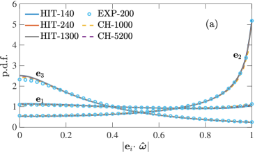
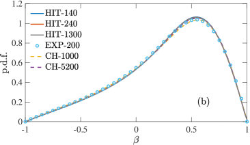
Figure 1a shows the probability density functions (PDFs) of the alignment cosines between vorticity and the strain eigenvectors: , where , for all the available data. It can be observed that the superposition between curves is nearly perfect. While ref. [21] already demonstrated -independence of these PDFs for HIT, our results here further demonstrate universality of these PDFs across different flows (at all ). A similar conclusion is drawn from Fig. 1b, which shows the PDF of , which provides a relative measure of with respect to the overall strain magnitude, with the constraint .
K41 hypothesizes that all small-scale statistics, including those of velocity gradients, are universal once rescaled by Kolmogorov length and time scales, respectively
| (1) |
We focus on the non-dimensional moments of longitudinal (diagonal) components of , i.e.,
| (2) |
for and repeated not implying summation. While K41 postulates that are constants, independent of , intermittency and extreme events lead to the following dependence:
| (3) |
Since local isotropy gives [11], it readily follows that and . but for , , and additionally, the constants are known to be flow-dependent [11, 12, 18].
To assess universality, we have extracted (up to ) from different flows. They are tabulated in Table 1 in the Appendix B, together with some other details; we reiterate the most important observations here. It is observed that local isotropy is valid for even moments of , i.e., are essentially independent of ; however, some persistent anisotropy is observed for the third moment or the skewness (and also higher order odd moments, which are not shown). As discussed in Appendix B, we instead consider an alternative skewness based on magnitude of vortex stretching, which is equal to when local isotropy holds [4, 21], but otherwise provides an average measure of skewnesses in three directions.
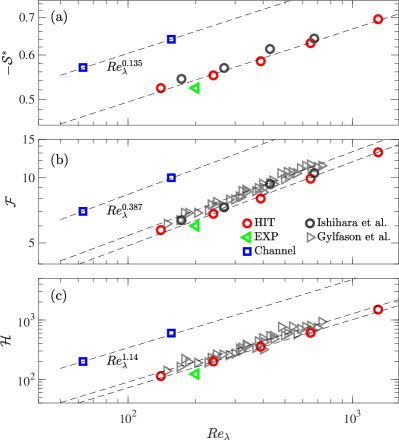
Figure 2a-c respectively show the scaling of skewness , flatness , and hyper-flatness as a function of . Remarkably, we observe that the scaling exponents are the same for all flows. While there is only one data point for newest experiments (EXP), we have also included previous experimental data from hot-wire measurements in grid turbulence [36], and also earlier HIT DNS at lower [9]. Since only one component is available from hot-wire measurements [36], we only consider even moments for this data 111as discussed in Appendix B, the third moments are not strictly isotropic and hence using the skewness of just could be misleading. On the other hand, only up to fourth moments are available from [9]. For all cases, the exponents , , are in excellent agreement with each other, with earlier HIT studies [36, 9, 38, 39], and also with predictions from intermittency theories [40, 11, 16, 38]. This confirms the universality of the scaling exponents in Eq. (3), with flow-dependent prefactors ; in agreement with the observations of [18], who considered scaling of dissipation moments in HIT, channel flow, and Rayleigh-Benard convection, albeit at lower than here 222see their Fig.4, where the data points are shifted to identify the same scaling exponents, but flow-dependent prefactors.
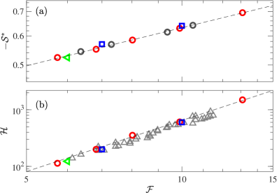
The above observation naturally leads to the question about the role of Reynolds number when comparing different flows. The ambiguity essentially arises from the fact that all Reynolds number definitions use , which is the large-scale velocity and hence, flow dependent. To resolve this ambiguity, we propose to use a small-scale quantity to characterize the turbulence intensity as opposed to Reynolds number, for instance, the skewness or flatness, which are both known to monotonically increase with . Figure 3a shows the plot of skewness vs. flatness, and Fig. 3b shows hyper-flatness vs. flatness, all taken from Fig. 2, which is in the spirit of extended self-similarity (ESS) [26]. Remarkably, we observe that data from all different flows collapses on a single curve (for both plots), which can be solely described by our HIT data.
The above result constitutes a substantially stronger evidence for universality than previously suggested [18]. Essentially, using Eq. (3), the result in Fig. 3a can be generally described
| (4) |
where the prefactors are also universal along with the exponents. Note, the choice of using as the dependent variable is somewhat arbitrary, and in principle, one can use any other moment. It is also worth mentioning here that recent Lagrangian results, see e.g. [38, 42], also similarly provide support for universality, but a more careful study is necessary, which we defer to future work.
The results in Fig. 3 suggests that the behavior of velocity gradients in HIT can be quantitatively extended to other flows (albeit in regions of no mean shear). However, one has to be mindful about matching the appropriate Reynolds numbers. Instead of simply matching the large-scale or Taylor-scale Reynolds, one has to match small-scale quantities such as skewness or flatness of velocity gradients. Based on this, we can readily see that the channel flow runs at and correspond to HIT runs at approximately and , respectively, substantially larger than the directly defined; whereas the from von Karman flow is slightly larger than in HIT. (Likewise, some minor shifting is required for grid turbulence data [36] and HIT data from [9]). With these considerations, we next investigate the structure and geometry of velocity gradient tensor, providing even stronger support for universality.
To gain deeper insight into extreme gradients, we separately analyze regions of intense vorticity and strain [21, 24, 29], by conditioning flow properties on:
| (5) |
where is the enstrophy and . In homogeneous flows, ; thus the extremeness of an event can be quantified by deviation of (or ) from unity. This has allowed us to analyze the structure of extreme events in HIT [10, 21, 24, 29, 31]. In the following, we compare key findings obtained from HIT with those from other flows.
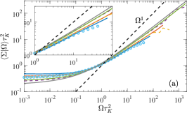
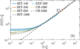
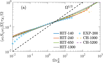
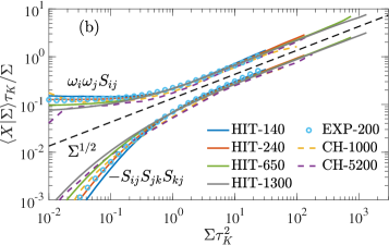
The first comparison is performed for the conditional expectations: and , which quantity the relative magnitudes of strain and vorticity in regions of intense vorticity and strain, respectively. In previous works, we showed that for HIT, (for ), where and grows slowly with ; additionally, the exponent can further be related to scaling of extreme events and smallest scales of turbulence [10, 24]. Figure 4a shows for all flows. We remarkably observe that the two curves for channel flow, at and , are essentially identical to HIT curves for and , respectively – in perfect agreement with earlier inferences from Fig. 3. This reiterates that extreme events are universal and depend only the turbulence intensity. The result for experiments is also in good agreement with HIT data, though there are some systematic deviations for the most extreme events, likely attributable to uncertainties associated with measuring them. On the other hand, it is known for HIT that [29, 24]. Figure 4b shows for all flows, and it can be seen that all curves collapse with a universal scaling.
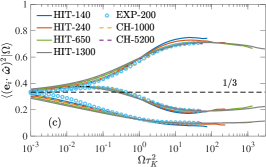
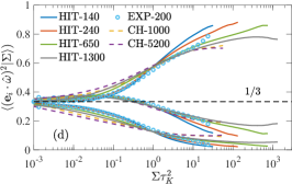
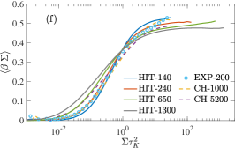
We next assess the universality of the structure of gradient tensor, by considering (as in Fig. 1) vorticity-strain alignments and the quantity . Figure 4c-d shows the second moments of alignment cosines, conditioned on and respectively. The second moment has the useful property: , allowing systematic characterization as a function of conditioning variable and also -dependence [21, 29]. Consistent with earlier results from HIT [21, 29], Fig. 4c-d, revealing excellent agreement between all flows, demonstrates that vorticity aligns even strongly with for extreme events. Additionally, all alignments are effectively -independent in regions of intense vorticity, and exhibit a weak -dependence in regions of intense strain.
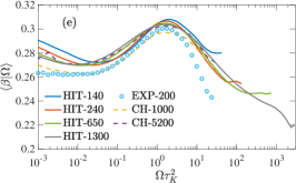
Figure 4e-f shows the expectations of , conditioned on and respectively. Once again, we obtain remarkable agreement between all flows, in support of universality 333There are some minor deviations for the experimental data, which can be attributed to difficulties in resolving large in experiments. The results effectively -independent in regions of intense vorticity, and exhibit a weak -dependence in regions of intense strain. Moreover, is nearly constant in regions of intense strain, and also larger than its value in regions of intense vorticity, where it slowly decreases (with ) – this behavior is readily explained by predominance of sheet-like structures for intense strain, and tube-like structures for intense vorticity [44, 23, 21]. Additional results on conditional vortex stretching and strain self-amplification are shown in Appendix C and also strongly support universality.
Discussion:
The K41 phenomenology posits universality of small scales, quantitatively characterized by the mean dissipation-rate. However, it well known that dissipation-rate and velocity gradients in general exhibit extreme fluctuations that invalidate K41’s mean-field description. We investigated the universality of extreme events by comparing their statistical properties across different turbulent flows, viz. isotropic turbulence, plane channel flow, and experiments in a von Karman mixing tank, also including some previous data from DNS [9] and grid-turbulence experiments [36]. Our first result is that the scaling exponents of velocity gradient moments, as a function of Reynolds number, are universal across different flows, extending the findings of [18] to higher Reynolds numbers. Using an approach in the spirit of extended self-similarity [26], we further demonstrate that even the proportionality constants are universal, provided the gradient moments are appropriately matched across flows, which occurs at different Reynolds numbers in different flows.
Thereafter, we present a detailed comparison of the structure of the velocity gradient tensor in different flows, by considering various statistics conditioned on extreme vorticity and strain. Once again, the results from isotropic turbulence are in near perfect quantitative agreement with those in other flows, once the Reynolds numbers are matched using prior results from gradient moments. Overall, our results reinforce small-scale universality for mean and extreme events alike. While K41’s mean-field description needs to replaced by intermittency models, our works show that results from isotropic turbulence can accurately characterize extreme events in other flows, extending well beyond the scope of scaling exponents alone. It also suggests that velocity gradients would serve as a more effective modeling target for capturing small-scale dynamics; such an approach could be particularly advantageous when leveraging machine learning techniques [45, 46], since they rely on directly learning from DNS data which are restricted to lower Reynolds.
Finally, it is worth noting that the observed universality in different flows is obtained far from boundaries and in regions of weak to no mean-shear (i.e., large-scale gradient). Given the evidence from other flows [47, 33, 6] and also scalar turbulence [48, 49, 50, 51], it appears that the presence of a large-scale mean-gradient persistently disrupt local isotropy and universality, even at high Reynolds numbers [33]. More effort is necessary to understand this effect in detail, and additionally develop intermittency theories capable of incorporating the effects of large-scale mean-gradients.
Acknowledgements.
Acknowledgments:
We gratefully acknowledge the Gauss Centre for Supercomputing e.V. (www.gauss-center.eu) for providing computing time on the supercomputers JUQUEEN and JUWELS at Jülich Supercomputing Centre (JSC), where the simulations reported in this paper were performed. We are very grateful to Eberhard Bodenschatz and Gerhard Nolte for making the experimental data available for processing, and also thank Armann Gylfason and Zellman Warhaft for sharing previous results, used in Figs.2-3.
References
- Kolmogorov [1941] A. N. Kolmogorov, Local structure of turbulence in an incompressible fluid for very large Reynolds numbers, Dokl. Akad. Nauk. SSSR 30, 299 (1941).
- Grant et al. [1962] H. L. Grant, R. W. Stewart, and A. Moilliet, Turbulence spectra from a tidal channel, J. Fluid Mech. 12, 241–268 (1962).
- Saddhoughi and Veeravalli [1994] S. Saddhoughi and S. V. Veeravalli, Local isotropy in turbulent boundary layers at high reynolds number, J. Fluid Mech. 268, 333–372 (1994).
- Kerr [1985] R. M. Kerr, Higher-order derivative correlations and the alignment of small-scale structures in isotropic numerical turbulence, J. Fluid Mech. 153, 31 (1985).
- van Atta [1991] C. van Atta, Local isotropy of the smallest scales of turbulent scalar and velocity fields, Proc. R. Soc. London A 434 (1991).
- Biferale and Procaccia [2005] L. Biferale and I. Procaccia, Anisotropy in turbulent flows and in turbulent transport, Phys. Reports 414 (2005).
- Meneveau and Sreenivasan [1991] C. Meneveau and K. R. Sreenivasan, The multifractal nature of turbulent energy dissipation, J. Fluid Mech. 224, 429– (1991).
- Jiménez et al. [1993] J. Jiménez, A. A. Wray, P. G. Saffman, and R. S. Rogallo, The structure of intense vorticity in isotropic turbulence, J. Fluid Mech. 255 (1993).
- Ishihara et al. [2007] T. Ishihara, Y. Kaneda, M. Yokokawa, K. Itakura, and A. Uno, Small-scale statistics in high resolution of numerically isotropic turbulence, J. Fluid Mech. 592, 335 (2007).
- Buaria et al. [2019] D. Buaria, A. Pumir, E. Bodenschatz, and P. K. Yeung, Extreme velocity gradients in turbulent flows, New J. Phys. 21, 043004 (2019).
- Frisch [1995] U. Frisch, Turbulence: the legacy of Kolmogorov (Cambridge University Press, Cambridge, 1995).
- Sreenivasan and Antonia [1997] K. R. Sreenivasan and R. A. Antonia, The phenomenology of small-scale turbulence, Annu. Rev. Fluid Mech. 29, 435 (1997).
- Wallace [2009] J. M. Wallace, Twenty years of experimental and direct numerical simulation access to the velocity gradient tensor: What have we learned about turbulence?, Phys. Fluids 21, 021301 (2009).
- Moin and Mahesh [1998] P. Moin and K. Mahesh, Direct numerical simulation: a tool in turbulence research, Annu. Rev. Fluid Mech. 30, 539 (1998).
- Paladin and Vulpiani [1987] G. Paladin and A. Vulpiani, Degrees of freedom of turbulence, Phys. Rev. A 35, 1971 (1987).
- Yakhot and Sreenivasan [2005] V. Yakhot and K. R. Sreenivasan, Anomalous scaling of structure functions and dynamic constraints on turbulence simulation, J. Stat. Phys. 121, 823 (2005).
- Yeung et al. [2018] P. K. Yeung, K. R. Sreenivasan, and S. B. Pope, Effects of finite spatial and temporal resolution in direct numerical simulations of incompressible isotropic turbulence, Phys. Rev. Fluids , in press (2018).
- Schumacher et al. [2014] J. Schumacher, J. D. Scheel, D. Krasnov, D. A. Donzis, V. Yakhot, and K. S. Sreenivasan, Small-scale universality in fluid turbulence, Proc. Natl. Acad. Sci. 111, 10961 (2014).
- Hamlington et al. [2012] P. E. Hamlington, D. Krasnov, T. Boeck, and J. Schumacher, Local dissipation scales and energy dissipation-rate moments in channel flow, J. Fluid Mech. 701 (2012).
- Ashurst et al. [1987] W. T. Ashurst, A. R. Kerstein, R. M. Kerr, and C. H. Gibson, Alignment of vorticity and scalar gradient with strain rate in simulated Navier-Stokes turbulence, Phys. Fluids 30, 2343 (1987).
- Buaria et al. [2020a] D. Buaria, E. Bodenschatz, and A. Pumir, Vortex stretching and enstrophy production in high Reynolds number turbulence, Phys. Rev. Fluids 5, 104602 (2020a).
- Tsinober [2009] A. Tsinober, An Informal Conceptual Introduction to Turbulence (Springer, Berlin, 2009).
- Buaria et al. [2020b] D. Buaria, A. Pumir, and E. Bodenschatz, Self-attenuation of extreme events in Navier-Stokes turbulence, Nat. Commun. 11, 5852 (2020b).
- Buaria and Pumir [2022] D. Buaria and A. Pumir, Vorticity-strain rate dynamics and the smallest scales of turbulence, Phys. Rev. Lett. 128, 094501 (2022).
- Knutsen et al. [2020] A. N. Knutsen, P. Baj, J. M. Lawson, E. Bodenschatz, J. R. Dawson, and N. A. Worth, The inter-scale energy budget in a von kármán mixing flow, Journal of Fluid Mechanics 895, A11 (2020).
- Benzi et al. [1993] R. Benzi, S. Ciliberto, R. Tripiccione, C. Baudet, F. Massaioli, and S. Succi, Extended self-similarity in turbulent flows, Phys. Rev. E 48, R29 (1993).
- Buaria and Sreenivasan [2020] D. Buaria and K. R. Sreenivasan, Dissipation range of the energy spectrum in high Reynolds number turbulence, Phys. Rev. Fluids 5, 092601(R) (2020).
- Buaria and Pumir [2021] D. Buaria and A. Pumir, Nonlocal amplification of intense vorticity in turbulent flows, Phys. Rev. Research 3, 042020 (2021).
- Buaria et al. [2022] D. Buaria, A. Pumir, and E. Bodenschatz, Generation of intense dissipation in high Reynolds number turbulence, Philos. Trans. R. Soc. A 380, 20210088 (2022).
- Buaria and Sreenivasan [2022a] D. Buaria and K. R. Sreenivasan, Intermittency of turbulent velocity and scalar fields using three-dimensional local averaging, Phys. Rev. Fluids 7, L072601 (2022a).
- Buaria and Pumir [2023] D. Buaria and A. Pumir, Role of pressure in the dynamics of intense velocity gradients in turbulent flows, J. Fluid Mech. 973, A23 (2023).
- Graham et al. [2016] J. Graham, K. Kanov, X. I. A. Yang, M. Lee, N. Malaya, C. C. Lalescu, R. Burns, G. Eyink, A. Szalay, R. D. Moser, and C. Meneveau., A web services accessible database of turbulent channel flow and its use for testing a new integral wall model for les, Journal of Turbulence 17, 181 (2016).
- Shen and Warhaft [2000] X. Shen and Z. Warhaft, The anisotropy of the small scale structure in high reynolds number turbulent shear flow, Phys. Fluids 12 (2000).
- Pumir et al. [2016] A. Pumir, H. Xu, and E. D. Siggia, Small-scale anisotropy in turbulent boundary layers, J. Fluid Mech. 804, 5 (2016).
- Betchov [1956] R. Betchov, An inequality concerning the production of vorticity in isotropic turbulence, J. Fluid Mech. 1, 497 (1956).
- Gylfason et al. [2004] A. Gylfason, S. Ayyalasomayajula, and Z. Warhaft, Intermittency, pressure and acceleration statistics from hot-wire measurements in wind-tunnel turbulence, J. Fluid Mech. 501, 213 (2004).
- Note [1] As discussed in Appendix B, the third moments are not strictly isotropic and hence using the skewness of just could be misleading.
- Buaria and Sreenivasan [2022b] D. Buaria and K. R. Sreenivasan, Scaling of acceleration statistics in high Reynolds number turbulence, Phys. Rev. Lett. 128, 234502 (2022b).
- Buaria and Sreenivasan [2023a] D. Buaria and K. R. Sreenivasan, Lagrangian acceleration and its Eulerian decompositions in fully developed turbulence, Phys. Rev. Fluids 8, L032601 (2023a).
- Kolmogorov [1962] A. N. Kolmogorov, A refinement of previous hypotheses concerning the local structure of turbulence in a viscous incompressible fluid at high Reynolds number, J. Fluid Mech. 13, 82 (1962).
- Note [2] See their Fig.4, where the data points are shifted to identify the same scaling exponents, but flow-dependent prefactors.
- Buaria and Sreenivasan [2023b] D. Buaria and K. R. Sreenivasan, Saturation and multifractality of Lagrangian and Eulerian scaling exponents in three-dimensional turbulence, Phys. Rev. Lett. 131, 204001 (2023b).
- Note [3] There are some minor deviations for the experimental data, which can be attributed to difficulties in resolving large in experiments.
- Moisy and Jiménez [2004] F. Moisy and J. Jiménez, Geometry and clustering of intense structures in isotropic turbulence, J. Fluid Mech. 513, 111 (2004).
- Tian et al. [2021] Y. Tian, D. Livescu, and M. Chertkov, Physics-informed machine learning of the Lagrangian dynamics of velocity gradient tensor, Phys. Rev. Fluids 6, 094607 (2021).
- Buaria and Sreenivasan [2023c] D. Buaria and K. R. Sreenivasan, Forecasting small-scale dynamics of fluid turbulence using deep neural networks, Proc. Natl. Acad. Sci. 120, e2305765120 (2023c).
- Pumir and Shraiman [1995] A. Pumir and B. Shraiman, Persistent small scale anisotropy in homogeneous shear flows, Phys. Rev. Lett. 75, 3114 (1995).
- Sreenivasan [1991] K. Sreenivasan, On local isotropy of passive scalars in turbulent shear flows, Proc. Roy. Soc. London. A 434 (1991).
- Pumir [1994] A. Pumir, Small-scale properties of scalar and velocity differences in three-dimensional turbulence, Phys. Fluids 6, 3974 (1994).
- Warhaft [2000] Z. Warhaft, Passive scalars in turbulent flows, Ann. Rev. Fluid Mech. 32 (2000).
- Buaria et al. [2021] D. Buaria, M. P. Clay, K. R. Sreenivasan, and P. K. Yeung, Small-scale isotropy and ramp-cliff structures in scalar turbulence, Phys. Rev. Lett. 126, 034504 (2021).
- Rogallo [1981] R. S. Rogallo, Numerical experiments in homogeneous turbulence, NASA Technical Memo (1981).
- Eswaran and Pope [1988] V. Eswaran and S. B. Pope, An examination of forcing in direct numerical simulations of turbulence, Comput. Fluids 16, 257 (1988).
- Buaria et al. [2024] D. Buaria, J. M. Lawson, and M. Wilczek, Twisting vortex lines regularize navier-stokes turbulence, Science Advances 10 (2024).
- Pope [2000] S. B. Pope, Turbulent Flows (Cambridge University Press, 2000).
Appendix A – Methods
DNS data:
The DNS data were obtained by solving the incompressible Navier-Stokes equations:
| (6) |
where is the divergence-free velocity , is the kinematic pressure, and is a large-scale forcing term, which depends on the flow considered.
The first flow considered is the canonical setup of forced isotropic turbulence with periodic boundary conditions, which allows us to use efficient and highly accurate Fourier pseudo-spectral methods [52]; The largest scales are forced isotropically to maintain a statistically stationary state [53]. The domain size is , discretized into grid points, with uniform grid-spacing in each direction. The Taylor-scale Reynolds number goes from to – as listed in Table 1, and special attention is given to resolve the small scales and extreme events [10], with . Additional details about the database can be found in several recent studies [21, 23, 27, 28, 29, 30, 31], which have also adequately established convergence with respect to resolution and statistical sampling.
The second flow considered is plane channel flow between two parallel plates (wall normal coordinate being ), forced by a constant mean pressure gradient. This data is obtained from the Johns Hopkins turbulence database [32], and corresponds to skin-friction Reynolds numbers and . Note, , where is the skin friction velocity and is the half-width of channel. For both cases, the domain size is , however, the grid spacing is not the same in each direction. Table 1 lists the grid spacing in each coordinate direction, at the center of the channel. It is worth noting that the resolution in the streamwise direction is for , and for . Earlier results from HIT [10] suggest that given the turbulence intensity of these flows, the resolution is not fully sufficient to capture the extreme events of velocity gradients (the component in this case). As discussed in Appendix B, this also appears to be the reason why the high order moments of are somewhat unpredicted.
Experimental data:
The experimental data were obtained at the center of a von Karman mixer, where the fluid is set to motion by two counter rotating impellers rotating at , with the axis of rotation assumed to be in the direction. The Taylor-scale Reynolds number is about . The apparatus and the data acquisition method are also described in [25, 54]. We note that the scanning Particle Image Velocimetry (PIV) technique allows us to obtain the full velocity field (and hence also the gradient field) in an observation volume of size , with , over a measurement grid-spacing of . Thus, each snapshot corresponds to about samples; about such snapshots of the flow where analyzed to obtain the desired statistics.
Appendix B – Local isotropy of velocity gradients
Small-scale isotropy or local isotropy is a prerequisite for universality [1, 11]. For the velocity gradient tensor, it can assessed rigorously by considering various moments of all nine components [55], but to keep things straightforward, we will focus on longitudinal (diagonal) components, (no summation implied) for . For local isotropy to be satisfied, one expects the moments to be identical for . This is indeed the case for HIT, and thus, we report only a single value in Table 1 for all HIT runs. However, for channel flow and experiments, we report three numbers for , to assess the validity of local isotropy.
As mentioned in the the main text, for , local isotropy dictates and thus . We observe in Table 1 that this is indeed the case, with some minor deviations for non-HIT runs, especially in experiments. For the skewness, given by , we observe more noticeable departures from isotropy for both channel flow and experiments, suggesting some effect of anisotropic large-scale forcing. Note that the skewness is different in -direction for both channel flow and experiments, consistent with direction of large-scale anisotropy. For channel flow, this effect seems to be diminishing with increasing , suggesting local isotropy would be strictly recovered at higher Reynolds number. The departure is more noticeable for experiments, likely because of presence of a weak mean-strain at the center of the tank [25].
Since the skewnesses for longitudinal components are not equal, we define , which measures vortex stretching and serves as an effective skewness; the rationale being that for local isotropy [21]. Alternatively, one can also use the quantity , which measures self-amplification of strain-rate [22]. In homogeneous turbulence, [35], and although not shown, this relation is near-perfectly satisfied for all the flows considered here.
| case | HIT-140 | HIT-240 | HIT-390 | HIT-650 | HIT-1300 | CH-1000 | CH-5200 | EXP-200 |
| - | - | - | - | - | 1000 | 5200 | - | |
| 140 | 240 | 390 | 650 | 1300 | 63 | 156 | 200 | |
| 0.5 | 0.5 | 0.5 | 0.5 | 0.5 | 2.2, 1.1, 1.1 | 1.5, 1.2, 0.8 | 0.8 | |
| 1.0 | 1.0 | 1.0 | 1.0 | 1.0 | 0.96, 1.03, 1.00 | 0.99, 1.01, 1.00 | 1.10, 0.90, 1.10 | |
| 0.524 | 0.552 | 0.585 | 0.630 | 0.695 | 0.439, 0.699, 0.468 | 0.579, 0.724, 0.589 | 0.750, 0.100, 0.775 | |
| 0.524 | 0.56 | 0.585 | 0.630 | 0.695 | 0.57 | 0.64 | 0.524 | |
| 5.74 | 6.82 | 8.02 | 9.90 | 13.1 | 6.44, 7.35, 6.80 | 9.70, 10.3, 10.0 | 6.2, 6.3, 6.2 | |
| 113 | 200 | 354 | 609 | 1495 | 134, 207, 161 | 472, 601, 626 | 122, 130, 118 |
Finally, we consider flatness
and hyper-flatness of the
gradients. Same as for , we observe that local
isotropy is reasonably satisfied for channel flow and experiments.
However, for channel flow, the hyper-flatness for is
noticeably lower. We believe this can be attributed
to lack of small-scale resolution in the -direction.
It can be seen from the table, that
for channel flow does not resolve adequately resolve
the Kolmogorov length scale [10].
For this reason, when considering the fourth moments,
we average over all three directions,
but for sixth moments for
channel flow, we simply take the average
over and directions for a reliable measure.
Given the restrictions on resolution and statistics
for non-HIT flows,
we refrain from considering moments higher than
in this work.
Appendix C – Universality of vortex stretching and strain self-amplification
To further add to the results presented in Fig. 4, we consider here the conditional expectations of the vortex stretching, , and strain self-amplification, , which appear in the transport equations for and [22, 21, 29]. Figure 5a shows for all flows, whereas Fig. 5b shows both terms conditioned on . Note that only vortex stretching is shown in Fig. 5a, since strain self-amplification does not contribute to vorticity amplification (but vortex stretching does play role in strain amplification).
A detailed discussion of the results in Fig. 5a-b and their implications, can be found in previous works [21, 29]; but it is worth noting that the qualitative behavior of the curves in Fig. 5a-b is quite similar to those in Fig. 4a-b, respectively. Essentially, the quantity grows as for extreme events, where as expected from a simple scaling relation between strain and vorticity. Moreover, the exponent weakly increases with Reynolds, slowly approaching the limiting value of . On the other hand, the quantities and both grow as for extreme events, with nearly no dependence on Reynolds number.
However, the key new observation is the agreement of results from different turbulent flows. Similar to previous result in Fig. 4a, we observe in Fig. 5b that the results for HIT at and are essentially identical to those from channel flow at and , respectively. In conclusion, the results in Fig. 5a-b once again strongly reinforce the universality of extreme events across different flows.