Importance Sampling With Stochastic Particle Flow and Diffusion Optimization
Abstract
\Acpfl is an effective method for overcoming particle degeneracy, the main limitation of particle filtering. In particle flow (PFL), particles are migrated towards regions of high likelihood based on the solution of a partial differential equation. Recently proposed stochastic PFL introduces a diffusion term in the ordinary differential equation (ODE) that describes particle motion. This diffusion term reduces the stiffness of the ODE and makes it possible to perform PFL with a lower number of numerical integration steps compared to traditional deterministic PFL. In this work, we introduce a general approach to perform importance sampling (IS) based on stochastic PFL. Our method makes it possible to evaluate a “flow-induced” proposal probability density function (PDF) after the parameters of a Gaussian mixture model (GMM) have been migrated by stochastic PFL. Compared to conventional stochastic PFL, the resulting processing step is asymptotically optimal. Within our method, it is possible to optimize the diffusion matrix that describes the diffusion term of the ODE to improve the accuracy-computational complexity tradeoff. Our simulation results in a highly nonlinear 3-D source localization scenario showcase a reduced stiffness of the ODE and an improved estimating accuracy compared to state-of-the-art deterministic and stochastic PFL.
I Introduction
The particle filter is probably the most widely used method for nonlinear sequential Bayesian estimation [1]. It can provide an asymptotically optimal approximation of posterior PDFs with complex shapes. The key operation performed in the update step of the particle filter is IS. Here, particles are first sampled from an arbitrary proposal PDF and then weighted based on the likelihood function. The particle filter is known to suffer from particle degeneracy in higher dimensional problems [2], i.e., due to the curse of dimensionality, too few particles have a significant weight after the update step.
To overcome particle degeneracy, PFL [3, 4] migrates particles sampled from a predicted/prior PDF to regions of high likelihood. By using a homotopy function, that describes the transition of the predicted/prior PDF to the posterior PDF, in the Fokker-Planck equation, one can either derive an ODE or stochastic differential equation (SDE) to describe the motion of particles. The resulting deterministic or stochastic PFLs have a zero or non-zero diffusion term, respectively. In particular, the exact Daum and Huang (EDH) flow [5] and the Gromov’s flow [6] are popular deterministic and stochastic flows with closed-form solutions. Stochastic flows tend to require a lower number of PFL steps due to improved transient dynamics, i.e., a reduced stiffness of the underlying ODE, and thus lead to a reduced overall computational complexity. As proposed and demonstrated recently [7], in stochastic PFL it is possible to optimize the diffusion term to further reduce stiffness and thus computational complexity. Although it has been demonstrated that PFL can overcome particle degeneracy in a variety of nonlinear and high-dimensional problems [3, 4, 5, 6], it has no asymptotical optimality guarantee [8].
The particle flow particle filter (PFPF)[8] embeds PFL into IS by introducing a flow-induced proposal PDF. The evaluation of this proposal at the migrated particles requires an invertible mapping from the predicted/prior PDF at particles before the flow and the PDF represented by the particles after the flow. Invertible deterministic PFL was recently combined with a GMM and used within a belief propagation framework for the 3-D tracking of an unknown number of sources in the presence of data association uncertainty [9, 10]. This approach has recently been used in the context of marine mammal research [11]. However, this invertible mapping is limited to deterministic flows like the EDH [12]. For stochastic PFL, in [12] particles are drawn at each flow step from a different proposal PDF, which leads to a computationally expensive weights computation for IS. The work in [13, 14] utilizes auxiliary variables and their filtering for IS with embedded PFL. In particular, [14] extended this framework to the stochastic Gromov’s flow. Although the method in [14] is computationally less expensive than [12], it has twice computational complexity of PFL due to an additional auxiliary variable for each particle. Furthermore, it relies on heuristic and suboptimal covariance matrix selections [14] and does not consider the most recent stochastic flows with optimized diffusion terms.
In this work, we introduce an approach that combines IS with general stochastic flows that include optimizable diffusion terms. The resulting IS framework is combined with a GMM and used within a belief propagation framework for the detection and localization of an unknown number of sources in 3-D. The main contributions of our work are summarized as follows.
-
•
We develop efficient IS where the parameters of a GMM are migrated by stochastic PFLs that rely on an SDE with an optimizable diffusion term.
-
•
We evaluate our method in a challenging 3-D multi-source localization problem and demonstrate significant improvements compared to state-of-the-art methods.
This paper advances over the preliminary account of our method provided in the conference publication [15] by (i) extending the approach to general stochastic flows that include optimizable diffusion terms and (ii) introducing additional and more extensive numerical results.
II Stochastic PFL
Consider a random state to be estimated, , in a Bayesian setting. PFL [3, 4] establishes a continuous mapping w.r.t. to pseudo-time , to migrate particles sampled from the the prior PDF such that they represent the posterior PDF .
Let be the prior PDF and be the likelihood function, where is observed and thus fixed. Following Bayes’ rule, a log-homotopy function [3, 4] can be introduced as . By using this log-homotopy function in the Fokker-Plank equation and modeling the dynamics of the particles by an SDE, i.e.,
| (1) |
stochastic PFLs can be derived [6]. (Note that modeling using an ODE, i.e., , leads to deterministic flows.)
In (1), is the drift vector, is the diffusion matrix, and is zero-mean Gaussian noise with covariance matrix . Since the drift is both time and state-dependent, directly integrating from 0 to 1 analytically is infeasible. Thus, the Euler-Maruyama method [16] is commonly used for numerical integration. Here, particle migration is performed by evaluating at discrete values of , i.e., . First, particles are drawn from . Next, each particle is migrated sequentially across the discrete pseudo time steps , i.e.,
| (2) |
where . In this way, particles representing the posterior PDF are finally obtained.
Recent results demonstrate that, based on an appropriate choice of the diffusion term , stochastic PFL can provide a strongly reduced number of integration steps and computational complexity compared deterministic PFL [7]. A popular stochastic flow is Gromov’s flow [6], given by the drift
| (3) |
and the diffusion matrix
| (4) |
Here, we used the short notation and .
For a linear measurement model with zero-mean additive Gaussian noise and covariance matrix , we have , , and . We can now rewrite drift (3) and diffusion (4) of Gromov’s flow as
For a nonlinear measurement model , one can linearize the measurement function at to obtain a linearized model. The Gromov’s flow applied to linearized measurement models has been demonstrated to outperform deterministic flows [14, 15, 17]. However, as other deterministic and stochastic PFLs, due to approximations made for numerical integration, the Gromov’s flow is not asymptotically optimal, i.e., the PDF represented by the particles after the flow is only an approximation of .
An alternative approach for asymptotically optimal estimation is to use PFL methods for IS within a particle filtering framework. Due to the lack of an invertible mapping in stochastic PFL, evaluating the PDF after the flow, as required for proposal evaluation [8], is typically infeasible.
III IS With Stochastic PFL
In this work, we propose to use PFL based on a linearized measurement model to develop a “flow-induced” GMM as proposal PDF. For example, let us first transform the drift of the Gromov flow to an affine function, i.e, , with
Next, consider a single Gaussian with mean and covariance matrix as predicted/prior PDF. Based on the affine form introduced above, we can migrate the mean and covariance of this Gaussian predicted/prior PDF based on PFL, i.e.,
| (5) | ||||
| (6) |
for and by setting and . This principle can be extended to GMMs in a straightforward way. The resulting “flow-induced” GMM can be used as a proposal PDF, leading to an IS method that makes it possible to perform efficient nonlinear estimation in an asymptotically optimal manner.
For an accurate numerical implementation of the PFL, the step sizes, , need to be adapted to the stiffness of the flow. A flow with reduced stiffness can be implemented with larger step sizes, i.e., fewer steps, and thus yields reduced computational complexity. Next, we investigate how to develop stochastic PFLs with reduced stiffness. Recently, it has been shown that a solution to (1) can be obtained by choosing arbitrarily and computing according to [7]
| (7) |
where is a deterministic flow, i.e. a solution of the ODE . Based on this result, one can choose a deterministic PFL and then design a diffusion matrix to get a stochastic PFL with reduced stiffness.
Consider the Gromov’s flow with stochastic drift and diffusion as in (3) and (4). Based on (7), the corresponding deterministic drift can be obtained as
| (8) |
By using an arbitrary diffusion matrix and by substituting in (7) by in (8), a new stochastic drift can be developed as
| (9) |
By considering a linearized measurement model, which results in , we can transform (9) to an affine function, i.e.,
| (10) |
Based on (5) and (6), this affine function can again be used to migrate the means and covariances of a GMM representing a predicted/prior PDF based on PFL.
The eigenvalues of the diffusion matrixes represent a tradeoff between the transient dynamics of the PFL and numerical evaluation accuracy. The freedom to choose makes it possible to optimize this tradeoff [7]. In particular, the transient dynamics of the PFL are measured by the condition number of the nonsingular matrix in (III), i.e., the ratio of the largest singular value to the smallest singular value of nonsingular . A small condition number close to one usually implies a reduced stiffness of the SDE [16]. Consider the following function form of in (III), i.e., where is a constant. We can get for . However, we cannot make too large, since it defines an upper bound of the numerical integration error using the Euler-Maruyama method [7].
To balance the stiffness reduction and the error of numerical evaluation of the SDE, we adapt the objective function [7]
| (11) |
where is a hyperparameter. The optimal solution obtained by minimizing (11) is , with
| (12) |
where and are the max and min of all eigenvalues of the Jacobian matrix of in (8), i.e., . For a detailed proof, see [7]. Recently, a simplified version of this solution has been introduced in [18]. This solution can offer higher computational efficiency in certain applications.
IV Numerical Experiments and Results
We evaluate our flow-induced proposal PDF in a 3-D source localization scenario where a volumetric array of receivers provides time-difference of arrival (TDOA) measurements [19]. This scenario is complicated by (i) the highly nonlinear TDOA measurement model, (ii) measurement-origin uncertainty, and (iii) an unknown number of sources to be localized [9, 10]. To address (ii) and (iii), we make use of the belief propagation (BP)-based message passing framework introduced in [20, 21]. To address (i), we use our flow-induced Gaussian mixture proposal PDF for weight computation in the belief update step and Monte Carlo integration in the message computation step. For more details on how PFL-based proposal PDF can be used within BP-based message passing framework, see [9, 10].
IV-A Source Localization Scenario and Implementation Aspects
In this work, we consider the localization of an unknown number of static sources in a 3-D region of interest (ROI). There are receivers. Pairs of receivers provide TDOA measurements, e.g., obtain by cross-correlation. In particular, the -th TDOA measurements provided by the receiver with index and the receiver with index , is modelled as
| (13) |
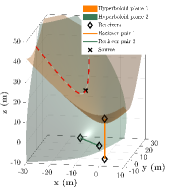
Here, and are the 3-D positions of the receivers, is the propagation speed in the considered medium, and is the additive white noise with variance . The noise is statistically independent across and across all receiver pairs . The dependence of a measurement on the source-location is described by the likelihood function that can be directly obtained from (13). Note that, due to the nonlinear TDOA measurement model, this likelihood function has the shape of a hyperboloid (cf. Fig. 1). For unambiguouse source localization, the measurements of multiple receiver pairs have to be used. Our scenario is further complicated by (ii) and (iii) discussed above.
Each receiver pair is considered one of sensors indexed by . The receivers of sensor are indexed and the number of measurements at sensor is . We consider a topology with receivers and sensors is shown in Fig. 1-b.
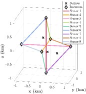
Furthermore, we set and . The clutter measurements at sensor follow a uniform PDF on . The mean number of clutter measurements is and the probability of source detection, , is set to . The ROI is defined as .
Following [20, 10], TDOA measurements are processed sequentially across sensors. More precisely, let be the multimodal posterior PDF after sensor update . This PDF is represented by Gaussian mixture components. For each component and each TDOA measurement, , of sensor , we perform PFL and update each kernel mean and covariance matrix based on (5) and (6). The resulting Gaussian components will be used for IS and Monte Carlo integration within BP-based message passing [20]. The result is an approximate posterior PDFs represented by Gaussian mixture components. For more details about BP message passing with PFL, see [10, 15].
As a reference methods for the proposed IS with optimized stochastic PFL (“PFL-OS”), we consider bootstrap IS (“BS”), which directly uses the posterior PDF from previous sensor as proposal PDF. We also use methods with “flow-induced” proposal PDFs using the deterministic EDH PFL (“PFL-D”) [10]) and the stochastic Gromov’s PFL (“PFL-S”) [15]). Since every method yields different stiffness, for numerical integration, every method requires a different resolution of the pseudo-time. This resolution is defined as the inverse of the time-interval . In addition, for every method, a higher resolution is typically needed at the first few steps of the numerical integration. We use an exponentially increasing ratio of the time-interval, i.e., , where is a fixed ratio for . Then, we control the interval by two parameters, the initial difference and the increasing ratio . Note that a larger and result in fewer discrete steps and thus to a reduced runtime. For each method, we choose and to obtain a good runtime-accuracy tradeoff .
IV-B Results
Table I shows the mean OSPA error [22] (with a cutoff threshold at 30) and runtime per run for the different methods and different parameters settings. OSPA and runtime are averaged over 100 Monte Carlo runs. We also list the number of Gaussian components, , as well as the number of samples per component, .
| ID | Method | OSPA | Runtime(s) | ||
|---|---|---|---|---|---|
| 1 | BS | ||||
| 2 | BS | ||||
| 3 | PFL-D | ||||
| 4 | PFL-S | ||||
| 5 | PFL-OS | ||||
| 6 | PFL-OS |
BS suffers from particle degeneracy and thus yields the highest OSPA. In addition, the large number of particles results in the largest memory requirements. In contrast, PFL-based methods required much fewer particles. It can be seen that, for the same value, PFL-S has a smaller OSPA error compared to PFL-D while its runtime is three times larger. PFL-OS relies on a diffusion matrix that has been minimized based on (11) by setting . Notably, PFL-OS yields the lowest OSPA error and, at the same time, has a low runtime.
To better understand the influence of on the estimation error for different step sizes, we compare the proposed methods for different values of and different resolutions of pseudo time. Results are shown in Table II. PFL-D and PFL-S results are also listed. When the step size is small, PFL can lead to accurate results despite the stiffness of the underlying ODEs and SDEs. In this case, traditional methods such as EDH and Gromov’s flow also perform well. However, the small step size comes at the cost of a strongly increased runtime. As the step size increases, only PFL-OS with carefully chosen parameter (cf. (11)) results in a good estimation accuracy. Importantly, our results indicate that PFL-OS has a significantly improved complexity accuracy tradeoff compared to PFL-D and PFL-S. Further numerical analysis is provided in [23]. Here, the tradeoff between the condition number of the Jacobian matrix and the norm of the diffusion matrix is analyzed numerically for different values of .
| PFL-D | 6.29 | 30 | 30 |
|---|---|---|---|
| PFL-S | 8.70 | 24.51 | 28.4 |
| PFL-OS () | 4.79 | 30 | 30 |
| PFL-OS () | 10.28 | 6.33 | 6.70 |
| PFL-OS () | 10.32 | 9.36 | 12.85 |
V Conclusion
In this paper, we introduced a general approach to perform IS based on stochastic PFL. Stochastic PFL introduces a diffusion term in the ODE that describes particle motion. A carefully determined diffusion term reduces the stiffness of the ODE and makes it possible to perform PFL with a lower number of numerical integration steps compared to traditional deterministic PFL. Our method makes it possible to evaluate a “flow-induced” proposal PDF after the parameters of a GMM have been migrated by stochastic PFL. Compared to conventional stochastic PFL, the resulting updating step is asymptotically optimal. Within our method, it is possible to optimize the diffusion matrix that describes the diffusion term of the ODE to improve the accuracy-computational complexity tradeoff. The presented numerical results in a highly nonlinear 3-D source localization scenario showcased a reduced stiffness of the ODE and an improved estimating accuracy compared to state-of-the-art deterministic and stochastic PFL. Further research includes flow-induced IS for different types of measurement models [24], application of flow-induced IS to real-world problems [25, 26], and efficient information-seeking control methods based on PFL [27, 28, 29].
References
- [1] M. S. Arulampalam, S. Maskell, N. Gordon, and T. Clapp, “A tutorial on particle filters for online nonlinear/non-Gaussian Bayesian tracking,” IEEE Trans. Signal Process., vol. 50, no. 2, pp. 174–188, Feb. 2002.
- [2] P. Bickel, B. Li, and T. Bengtsson, “Sharp failure rates for the bootstrap particle filter in high dimensions,” in Pushing the Limits of Contemporary Statistics: Contributions in Honor of Jayanta K. Ghosh, vol. 3. Beachwood, OH, USA: Inst. Math. Statist., 2008, pp. 318–329.
- [3] F. Daum and J. Huang, “Nonlinear filters with log-homotopy,” in Proc. SPIE-07, Aug. 2007, pp. 423–437.
- [4] ——, “Nonlinear filters with particle flow induced by log-homotopy,” in Proc. SPIE-09, May 2009, pp. 76–87.
- [5] F. Daum, J. Huang, and A. Noushin, “Exact particle flow for nonlinear filters,” in Proc. SPIE-10, Apr. 2010, pp. 92–110.
- [6] ——, “New theory and numerical results for Gromov’s method for stochastic particle flow filters,” in Proc. FUSION-18, 2018, pp. 108–115.
- [7] L. Dai and F. Daum, “On the design of stochastic particle flow filters,” IEEE Trans. Aerosp. Electron. Syst., vol. 59, no. 3, pp. 2439–2450, 2023.
- [8] Y. Li and M. Coates, “Particle filtering with invertible particle flow,” IEEE Trans. Signal Process., vol. 65, no. 15, pp. 4102–4116, Aug. 2017.
- [9] W. Zhang and F. Meyer, “Graph-based multiobject tracking with embedded particle flow,” in Proc. IEEE RadarConf-21, Atlanta, GA, USA, May 2021.
- [10] ——, “Multisensor multiobject tracking with improved sampling efficiency,” IEEE Trans. Signal Process., vol. 72, pp. 2036–2053, 2024.
- [11] J. Jang, F. Meyer, E. R. Snyder, S. M. Wiggins, S. Baumann-Pickering, and J. A. Hildebrand, “Bayesian detection and tracking of odontocetes in 3-D from their echolocation clicks,” J. Acoust. Soc. Am., vol. 153, no. 5, p. 2690–2705, May 2023.
- [12] P. Bunch and S. Godsill, “Approximations of the optimal importance density using Gaussian particle flow importance sampling,” J. Amer. Statist. Assoc., vol. 111, no. 514, pp. 748–762, Aug. 2016.
- [13] Y. Li, L. Zhao, and M. Coates, “Particle flow auxiliary particle filter,” in Proc. IEEE CAMSAP-15, Cancun, Mexico, Dec. 2015, pp. 157–160.
- [14] S. Pal and M. Coates, “Particle flow particle filter using Gromov’s method,” in Proc. IEEE CAMSAP-19, Guadeloupe, France, Dec. 2019, pp. 634–638.
- [15] W. Zhang, M. J. Khojasteh, and F. Meyer, “Particle flows for source localization in 3-D using TDOA measurements,” in Proc. FUSION-24, Venice, Italy, 2024.
- [16] P. E. Kloeden and E. Platen, Numerical Solution of Stochastic Differential Equations. Berlin, Germany: Springer, 1992.
- [17] D. F. Crouse, “Particle flow filters: Biases and bias avoidance,” in Proc. FUSION-22, Ottawa, Canada, 2019, pp. 1–8.
- [18] F. Daum, L. Dai, J. Huang, and A. Noushin, “Bullet proofing bayesian particle flow against stiffness,” in Signal Processing, Sensor/Information Fusion, and Target Recognition XXXIII, vol. 13057. SPIE, 2024, pp. 62–71.
- [19] F. Gustafsson and F. Gunnarsson, “Positioning using time-difference of arrival measurements,” in Proc. IEEE ICASSP-03, vol. 6, Hong Kong, China, Apr. 2003, pp. 553–556.
- [20] F. Meyer, T. Kropfreiter, J. L. Williams, R. A. Lau, F. Hlawatsch, P. Braca, and M. Z. Win, “Message passing algorithms for scalable multitarget tracking,” Proc. IEEE, vol. 106, no. 2, pp. 221–259, Feb. 2018.
- [21] F. Meyer, P. Braca, P. Willett, and F. Hlawatsch, “A scalable algorithm for tracking an unknown number of targets using multiple sensors,” IEEE Trans. Signal Process., vol. 65, no. 13, pp. 3478–3493, Jul. 2017.
- [22] D. Schuhmacher, B.-T. Vo, and B.-N. Vo, “A consistent metric for performance evaluation of multi-object filters,” IEEE Trans. Signal Process., vol. 56, no. 8, pp. 3447–3457, 2008.
- [23] W. Zhang, M. J. Khojasteh, N. A. Atanasov, and F. Meyer, “Importance sampling with stochastic particle flow and diffusion optimization: Supporting results,” 2024, https://fmeyer.ucsd.edu/SPL-2024-SR.pdf.
- [24] F. Meyer and J. L. Williams, “Scalable detection and tracking of geometric extended objects,” IEEE Trans. Signal Process., vol. 69, pp. 6283–6298, Oct. 2021.
- [25] M. Liang and F. Meyer, “Neural enhanced belief propagation for multiobject tracking,” IEEE Trans. Signal Process., vol. 72, pp. 15–30, 2024.
- [26] L. Watkins, P. Stinco, A. Tesei, and F. Meyer, “A probabilistic focalization approach for single receiver underwater localization,” in Proc. FUSION-24, Venice, Italy, 2024.
- [27] W. Zhang, B. Teague, and F. Meyer, “Active planning for cooperative localization: A Fisher information approach,” in Proc. Asilomar-22, Pacific Grove, CA, USA, 2022, pp. 795–800.
- [28] J. A. Placed, J. Strader, H. Carrillo, N. Atanasov, V. Indelman, L. Carlone, and J. A. Castellanos, “A survey on active simultaneous localization and mapping: State of the art and new frontiers,” IEEE Trans. Robot., vol. 39, no. 3, pp. 1686–1705, 2023.
- [29] A. Asgharivaskasi and N. Atanasov, “Semantic OcTree mapping and shannon mutual information computation for robot exploration,” IEEE Trans. Robot., vol. 39, no. 3, pp. 1910–1928, 2023.