Private Synthetic Data Generation in Small Memory

Abstract

Protecting sensitive information on data streams is a pivotal challenge for modern systems. Current approaches to providing privacy in data streams can be broadly categorized into two strategies. The first strategy involves transforming the stream into a private sequence of values, enabling the subsequent use of non-private methods of analysis. While effective, this approach incurs high memory costs, often proportional to the size of the database. Alternatively, a compact data structure can be used to provide a private summary of the stream. However, these data structures are limited to predefined queries, restricting their flexibility.

To overcome these limitations, we propose a novel lightweight synthetic data generator, $\mathtt{PrivHP}$, that provides differential privacy guarantees in a resource-efficient manner. Our approach generates private synthetic data that preserves the underlying distribution of the original stream, allowing for flexible downstream analyses without incurring additional privacy costs. $\mathtt{PrivHP}$ leverages a hierarchical decomposition of the input domain, selectively pruning low-frequency subdomains while preserving high-frequency subdomains, which are identified and managed in a privacy-preserving fashion. To ensure memory efficiency in a streaming context, we employ private sketches to estimate subdomain frequencies without accessing the entire dataset. Utilizing this combination of hierarchical pruning and frequency approximation, $\mathtt{PrivHP}$ is the first solution for synthetic data generation that balances privacy, memory efficiency, and utility.

$\mathtt{PrivHP}$ is parameterized by a privacy budget $\varepsilon$, a pruning parameter $k$ and the sketch width $w$. It can process a dataset of size $n$ in $\mathcal{O}((w+k)\log(\varepsilon n))$ space, $\mathcal{O}(\log(\varepsilon n))$ update time and outputs a private synthetic data generator in $\mathcal{O}(k\log k\log(\varepsilon n))$ time. All prior methods require $\Omega(n)$ space and (if adapted to a stream) $\Omega(n)$ construction time. We evaluate the utility of our approach by measuring the expected 1-Wasserstein distance between the sampler and the empirical distribution of the input. Compared to state-of-the-art methods, we demonstrate that the additional cost in utility is inversely proportional to $k$ and $w$. This is the first meaningful trade-off between performance and utility for private synthetic data generation.

Keywords Differential Privacy  $\cdot$ Synthetic Data  $\cdot$ Data Streaming

1 Introduction

A data stream solution addresses the problem of analyzing large volumes of data with limited resources. Numerous techniques have been developed to enable real-time analytics with minimal memory usage and high throughput [1, 2, 3]. However, if the stream contains sensitive information, privacy concerns become paramount [4, 5]. In such cases, a data stream solution must optimize resource efficiency while balancing utility and strong privacy protection.

The concept of differential privacy has emerged as the prevailing standard for ensuring privacy in the analysis of data streams. It guarantees that an observer analyzing the outputs of a differentially private algorithm is fundamentally limited, in an information-theoretic sense, in their ability to infer the presence or absence of any individual data point in the stream. Methods for supporting differentially private queries on data streams can be broadly categorized into two strategies. The first strategy transforms the data stream into a differentially private sequence of values or statistics, which can subsequently be processed and queried by non-private data structures [6, 7, 8, 5]. However, these approaches can incur high memory costs, limiting their applicability in many streaming contexts. The second approach involves constructing specialized data structures, with small memory allocations, that provide differentially private answers to specific, predefined queries [9, 10, 11]. Although this approach is memory efficient, it restricts the range of queries to those selected in advance, reducing flexibility.

To address these limitations, we propose a lightweight synthetic data generator, $\mathtt{PrivHP}$ (Private Hot Partition), that provides differential privacy and operates with high throughput and in small memory. Our generator produces private synthetic data that approximates the distribution of the original data stream. This synthetic data can be used for any downstream task without additional privacy costs. Therefore, $\mathtt{PrivHP}$ protects sensitive information and supports a broad range of queries in resource-constrained environments.

1.1 Problem and Solution

Mathematically, the problem of generating synthetic data can be defined as follows. Let $(\Omega,\rho)$ be a metric space and consider a stream $\mathcal{X}=(X_{1},\ldots,X_{n})\in\Omega^{n}$. Our goal is to construct a space and time-efficient randomized algorithm that outputs synthetic data $\mathcal{Y}=(Y_{1},\ldots,Y_{m})\in\Omega^{m}$, such that the two empirical measures

$$\mu_{\mathcal{X}}=\frac{1}{n}{\sum_{i=1}^{n}}\delta_{X_{i}}\quad\text{and}\quad\mu_{\mathcal{Y}}=\frac{1}{m}{\sum_{i=1}^{m}}\delta_{Y_{i}}$$

are close together. Moreover, the output $\mathcal{Y}$ should satisfy differential privacy.

Our approach adapts recent advancements in private synthetic data generation (in a non-streaming setting) that utilizes a hierarchical decomposition to partition the sample space [12, 13]. At a high level, these methods work in the following way:

1. Hierarchically split the sample space into subdomains;

2. For each subdomain, count how often items from the dataset appear within it;

3. To ensure privacy, add a carefully chosen amount of random noise to each frequency count;

4. Use these noisy counts to construct a probability distribution so that items from each subdomain can be sampled with a probability proportional to their noisy frequency.

The accuracy of this approach depends on the granularity of the partition. Creating more subdomains of smaller diameter can improve the approximation of the real distribution, but requires more memory. Therefore, the challenge of constructing a high-fidelity partition on a stream is this balance between granularity and memory.

To meet this challenge, $\mathtt{PrivHP}$ adopts a novel method for hierarchical decomposition that prunes less significant subdomains while prioritizing subdomains with a high frequency of items. In addition, we use sketching techniques to approximate frequencies at deeper levels in the hierarchy, allowing for effective pruning without requiring access to the entire dataset. Similar to He et al. [12], to maintain privacy, we perturb the frequency counts of nodes in the (pruned) hierarchy.

1.2 Main Result

We measure the utility of a synthetic data generator $\mathcal{T}$ by $\mathbb{E}[W_{1}(\mu_{\mathcal{X}},\mathcal{T})]$, where $W_{1}(\mu_{\mathcal{X}},\mathcal{T})$ is the 1-Wasserstein metric, and $\mathbb{E}$ is taken over the randomness of the algorithm generating $\mathcal{T}$. Our results explore trade-offs between utility and performance. We are interested in quantifying the cost, in utility, of supporting synthetic data generation under resource constraints. To this end, $\mathtt{PrivHP}$ is instantiated with a pruning parameter $k$ and a sketch parameter $w$. Both allow for increased accuracy at the expense of more memory. This is formalized in the following result on the hypercube $\Omega=[0,1]^{d}$.

Theorem 1.

When $\Omega=[0,1]^{d}$ equipped with the $l^{\infty}$ metric, for sketch parameter $w$ and pruning parameter $k$, $\mathtt{PrivHP}$ can process a stream $\mathcal{X}$ of size $n$ in $\mathcal{O}((w+k)\log(\varepsilon n))$ memory and $\mathcal{O}(\log(\varepsilon n))$ update time. $\mathtt{PrivHP}$ can subsequently output a $\varepsilon$-differentially private synthetic data generator $\mathcal{T}_{\mathtt{PrivHP}}$, in $\mathcal{O}(k\log k\log\varepsilon n)$ time, such that

$$\mathbb{E}[W_{1}(\mu_{\mathcal{X}},\mathcal{T}_{\mathtt{PrivHP}})]=\begin{cases}\mathcal{O}\left(\frac{\log^{2}(k)}{\varepsilon n}+k^{-1}(w^{-1}+f(\mathcal{X},k))\right)&\text{if }d=1\\ \mathcal{O}\left(\frac{k^{(1-\frac{1}{d})}}{\varepsilon n}+{k^{-\frac{1}{d}}}(w^{-1}+f(\mathcal{X},k))\right)&\text{if }d\geq 2\end{cases},$$

where $f$ is a function that depends only on the input dataset and the pruning parameter $k$. Moreover,

$$f(\mathcal{X},k) =\begin{cases}\mathcal{O}(1)&\text{if }\mathcal{X}\sim\mathtt{Uniform}([0,1]^{d})\\ \mathcal{O}(1-B)&\text{if }\mathcal{X}\sim\mathtt{MultiFractal}(B,[0,1]^{d})\end{cases}$$

The function $f$ is used to capture the influence of the input distribution on utility. The $\mathtt{MultiFractal}$ distribution is used to model skew in the input stream. Our result demonstrates that the utility of our generator improves when there is more skew (that is, when $B$ increases) in the stream.

For comparison, the state-of-the-art for $d=1$ achieves a utility bound of $\mathcal{O}(\log^{2}(\varepsilon n)(\varepsilon n)^{-1})$ in a memory cost that is $\mathcal{O}(\varepsilon n)$ [12]. Therefore, the second term in our bound, $k^{-1}(w^{-1}+f(\mathcal{X},k))$, quantifies the cost introduced by moving to a smaller memory solution. Either increasing the size of the sketches $w$, supporting more accurate frequency estimates, or increasing the pruning parameter $k$, supporting a larger partition of the sample space, enables improved utility at the cost of more memory. A full comparison with prior work is provided in Table 1.

Our contributions can be summarized as follows. We introduce the first data structure that supports private synthetic data generation with provable utility bounds in resource-constrained environments. This advancement establishes meaningful trade-offs between utility and resource usage, enabling a balanced configuration tailored to diverse application settings. This extends the domain for private synthetic data generation to low-memory, high-throughput data streams. In this context, high fidelity synthetic data sets, with formal privacy guarantees, can be generated and applied to a variety of downstream data analysis tasks.

1.3 Organization of the Paper

As background, Section 2 covers related work and Section 3 establishes the relevant preliminaries. Section 4 presents material relevant to sketching and contains a proof that is used in subsequent analysis. Section 5 introduces our method for compact hierarchical decompositions on the stream. Section 6 covers synthetic data generation using hierarchical partitions and supplies the main results. Section 7 discusses our approach for measuring utility using the 1-Wasserstein distance. Section 8 contains the proof of a more general version of Theorem 1. Lastly, Section 9 extends the previous section to the hypercube and contains the proof of Theorem 1.

2 Related Work

2.1 Non-Streaming Private Synthetic Data Generation

The problem of generating private synthetic data from static datasets, especially in relation to differential privacy, has been explored in depth. The challenge of this problem was demonstrated by Ullman and Vadhan, who showed that, given assumptions on one-way functions, generating private synthetic data for all two-dimensional marginals is NP-hard on the Boolean cube [14]. Research has since focused on guaranteeing privacy for specific query sets [15, 16, 17, 18, 19, 20].

Method	Accuracy		Memory
	$\Omega=[0,1]$	$\Omega=[0,1]^{d},d\geq 2$
$\mathtt{Smooth}$ [21]	$\mathcal{O}\left(\varepsilon^{-1}n^{-K/(2d+K)}\right)$		$\mathcal{O}(dn)$
$\mathtt{SRRW}$ [22]	$\mathcal{O}\left(\left({\log^{\frac{3}{2}}(\varepsilon n)}{(\varepsilon n)^{-1}}\right)^{1/d}\right)$		$\mathcal{O}(dn)$
$\mathtt{PMM}$ [12]	$\mathcal{O}\left({\log^{2}(\varepsilon n)}{(\varepsilon n)^{-1}}\right)$	$\mathcal{O}\left((\varepsilon n)^{-1/d}\right)$	$\mathcal{O}(\varepsilon n)$
$\mathtt{PrivHP}$	$\mathcal{O}\left(\frac{\log^{2}(k)}{\varepsilon n}+k^{-1}(w^{-1}+f(\mathcal{X},k))\right)$	$\mathcal{O}\left(\frac{k^{(1-\frac{1}{d})}}{\varepsilon n}+k^{-\frac{1}{d}}(w^{-1}+f(\mathcal{X},k))\right)$	$\mathcal{O}((w+k)\log\varepsilon n)$

Table 1: Performance of $\mathtt{PrivHP}$ vs prior work. Results are presented for input domains $\Omega=[0,1]$ and $\Omega=[0,1]^{d}$ ($d\geq 2$). Accuracy is measured by the expected 1-Wasserstein distance. The utility guarantee for $\mathtt{Smooth}$ is restricted to smooth queries with bounded partial derivatives of order $K$. The function $f(\mathcal{X},k)$ is a constant when the input follows a $\mathtt{Uniform}$ distribution and is equal to $\mathcal{O}(1-B)$ when the input follows a $\mathtt{MultiFractal}$ distribution with skew parameter $B$.

The utility for private synthetic data is measured by the expected 1-Wasserstein distance. Wang et al. [21] addressed private synthetic data generation on the hypercube $[0,1]^{d}$. They introduced a method ($\mathtt{Smooth}$) for generating synthetic data that comes with a utility guarantee for smooth queries with bounded partial derivatives of order $K$, achieving accuracy $\mathcal{O}(\varepsilon^{-1}n^{-K/(2d+K)})$. More recently, Boedihardjo et al. [22] proved an accuracy lower bound of $\mathcal{O}(n^{-1/d})$. They also introduced an approach ($\mathtt{SRRW}$) based on super-regular random walks with near-optimal utility of $\mathcal{O}(\log^{3/2}(\varepsilon n)(\varepsilon n)^{-1/d})$. Subsequently, He et al. [12] proposed an approach $\mathtt{PMM}$, based on hierarchical decomposition, that achieves optimal accuracy (up to constant factors) for $d\geq 2$. These methods provide a combination of privacy and provable utility. However, they do not consider resource constraints. In contrast, our approach provides meaningful trade-offs between utility and resources. A summary of accuracy vs. memory for prior work is presented in Table 1.

2.2 Privacy on Data Streams

A common strategy for supporting privacy on streams is to transform the stream into a differentially private sequence of values [6, 8, 5]. While this enables query flexibility, current methods require storing the full stream in memory. This limits its application in resource-constrained environments. In the traditional data steam model, where memory is sublinear in the size of the database, the current approach for protecting streams is to construct specialized data structures, with small memory allocations, that provide differentially private answers to specific, predefined queries [9, 10, 11]. However, these methods lack query flexibility.

$L_{p}$-sampling methods are central to data streaming algorithms, and can support a wide range of queries with low memory usage [23, 24, 25, 26, 3]. These techniques come with formal accuracy guarantees and can be made private with the use of private linear sketches [11]. In addition, a private $L_{p}$-sampler could be used to generate synthetic data by partitioning the sample space $\Omega$ into small disjoint portions $\Omega_{1},\Omega_{2},\ldots,\Omega_{n}$ and sampling these portions according to their relative frequencies. If the sampler returns some subdomain $\Omega_{i}$, we can then return any element $x\in\Omega_{i}$. However, each sampler can only return 1 item for its utility guarantee to hold. Therefore, the size of the sample needs to be known in advance. In contrast, $\mathtt{PrivHP}$ can generate an unlimited amount of synthetic data at a fixed memory allocation.

2.3 Private Hierarchical Decomposition

Many methods for hierarchical decomposition have been adapted to the context of differential privacy [27, 7, 28, 29]. Static solutions, such as $\mathtt{PrivTree}$ [29], require full access to the dataset and are not suitable for streaming. The dynamic decomposition introduced by $\mathtt{PrivStream}$ [7] adapts $\mathtt{PrivTree}$ to the stream. However, $\mathtt{PrivStream}$ is supported by a fixed and potentially large hierarchical partition of the input domain that must be stored locally with exact counts [7, 5]. Therefore, it incurs large memory costs and is not suited to resource-constrained settings. We overcome this limitation by adopting pruning and sketching techniques to summarize deeper levels of the hierarchy. In addition, $\mathtt{PrivStream}$ does not provide any utility guarantees.

Biswas et al. introduced a streaming solution for hierarchical heavy hitters [9] that, similar to our approach, supports a private hierarchical decomposition on the stream. Thus, their technique could be used for private synthetic data generation. Our approach has two differences. We adopt a different pruning criteria, which enables better worst-case performance, and a different sketching technique, which supports more accurate frequency estimation. In Appendix D, we elaborate on why our approach achieves a better utility guarantee for synthetic data generation.

3 Preliminaries

3.1 Privacy

Differential privacy ensures that the inclusion or exclusion of any individual in a dataset has a minimal and bounded impact on the output of a mechanism. Two streams $\mathcal{X}$ and $\mathcal{X}^{\prime}$ are neighboring, denoted $\mathcal{X}\sim\mathcal{X}^{\prime}$, if they differ in one element. Formally, $\mathcal{X}\sim\mathcal{X}^{\prime}$ if $\mathcal{X}^{\prime}=\mathcal{X}$. $x_{i}\neq x_{i}^{\prime}$. The following definition of differential privacy is from Dwork and Roth [30].

Definition 1 (Differential Privacy).

A randomized mechanism $\mathcal{M}$ satisfies $\varepsilon$-differential privacy if and only if for all pairs of neighboring streams $\mathcal{X}\sim\mathcal{X}^{\prime}\in\Omega^{*}$ and all measurable sets of outputs $Z\subseteq\mathtt{support}(\mathcal{M})$ it holds that

$$\textup{{Pr}}[\mathcal{M}(\mathcal{X})\in Z]\leq e^{\varepsilon}\textup{{Pr}}[\mathcal{M}(\mathcal{X}^{\prime})\in Z]$$

The Laplace mechanism is a fundamental technique for ensuring differential privacy by adding noise calibrated to a function’s sensitivity. Let $\triangle_{p}(f)=\max_{\mathcal{X}\sim\mathcal{X}^{\prime}}\lVert f(\mathcal{X})-f(\mathcal{X}^{\prime})\rVert_{p}$ denote the $p$-sensitivity of the function $f$.

Lemma 1 (Laplace Mechanism).

Let $f$ be a function with $L_{1}$-sensitivity $\triangle_{1}(f)$. The mechanism

$$\mathcal{M}(\mathcal{X})=f(\mathcal{X})+\mathtt{Laplace}\left(\frac{\triangle_{1}(f)}{\varepsilon}\right),$$

satisfies $\varepsilon$-differential privacy, where $\mathtt{Laplace}$ is a Laplace distribution with mean 0 and scale parameter $\frac{\triangle_{1}(f)}{\varepsilon}$.

Differential privacy is preserved under certain operations on private mechanisms, particularly post-processing and composition, which make it a robust privacy model. A significant property of differential privacy is that it is invariant under post-processing. This means that applying any deterministic or randomized function to the output of an $\varepsilon$-differentially private mechanism does not decrease its privacy guarantee.

Lemma 2 (Post-Processing).

If $\mathcal{M}$ is an $\varepsilon$-differentially private mechanism and $g$ is any randomized mapping, then $g\circ\mathcal{M}$ is also $\varepsilon$-differentially private.

Differential privacy is also preserved under composition. When multiple differentially private mechanisms are applied to the same data, the total privacy loss accumulates. The composition property quantifies this cumulative privacy loss, providing bounds for combining mechanisms.

Lemma 3 (Basic Composition).

If $\mathcal{M}_{1}$ and $\mathcal{M}_{2}$ are $\varepsilon_{1}$- and $\varepsilon_{2}$-differentially private mechanisms, respectively, then the mechanism defined by their joint application, $(\mathcal{M}_{1},\mathcal{M}_{2})$, is $(\varepsilon_{1}+\varepsilon_{2})$-differentially private.

3.2 Utility

The utility of the output is measured by the expectation of the 1-Wasserstein distance between two measures:

$$\mathcal{W}_{1}(\mu_{\mathcal{X}},\mu_{\mathcal{Y}})=\sup_{\textsf{Lip}(f)\leq 1}\left(\int fd\mu_{\mathcal{X}}-\int fd\mu_{\mathcal{Y}}\right),$$ (1)

where the supremum is taken over all 1-Lipschitz functions on $\Omega$. Since many machine learning algorithms are Lipschitz [31, 32], Equation 1 provides a uniform accuracy guarantee for a wide range of machine learning tasks performed on synthetic datasets whose empirical measure is close to $\mu_{\mathcal{X}}$ in the 1-Wasserstein distance.

3.3 Multi-fractal distribution

We examine the utility of our technique under different input distributions, demonstrating that utility improves if skew is present in the data stream. We consider the multi-fractal distribution as a model for skew. Previously, multifractals have been used to model the address space in IP traffic [33, 34]. A multifractal distribution with parameter $B$ on a sample space $\Omega$ is constructed by iteratively splitting $\Omega$ into subsets $\Omega_{0},\Omega_{1},\dots$ with probabilities governed by $B\in[1/2,1]$. Initially, $\Omega$ splits into $\Omega_{0}$ and $\Omega_{1}$ with probabilities

$$\textup{{Pr}}(\Omega_{0})=B\quad\text{and}\quad\textup{{Pr}}(\Omega_{1})=1-B.$$

This process recurses within each subset, creating a hierarchical, self-similar distribution where the parameter $B$ controls the concentration of probability in specific regions.

4 Sketching

Our generator relies on a partition of the sample space. Prior works, such as $\mathtt{PrivTree}$ and $\mathtt{PMM}$, construct partitions using exact frequency counts, which require access to the full dataset. For compact partitions, we instead use approximate frequency counts that are private and support private Top-$k$ selection. We adopt private sketches [35, 11] to meet these needs.

A sketch performs a random linear transformation $A$ to embed a vector $X\in\mathbb{R}^{n}$ into a smaller domain $AX\in\mathbb{R}^{j\times w}$. When the embedding dimension $j\times w$ is small, memory is reduced at the cost of increased error. A private sketch adds noise to the transformation to make the distribution of the sketch indistinguishable on neighboring inputs. Common examples are the Private Count Sketch and Private Count-Min Sketch [35, 11]. They share a similar structure but differ in their update and query procedures. We first overview non-private variants of sketches and then demonstrate how to apply differential privacy.

The Count-Min Sketch [36] is a $j\times w$ matrix of counters, $C(X)\in\mathbb{R}^{j\times w}$, determined by random hash functions $h_{1},\ldots,h_{j}:[n]\rightarrow[w]$, where each $h_{i}$ maps entries $x\in X$ into a bucket $h_{i}(x)$ within row $i$. For $(i,k)\in[j]\times[w]$, each bucket is defined as:

$$C(X)_{i,k}=\sum_{x\in X}x\cdot\mathbbm{1}(h_{i}(x)=k),$$

where $\mathbbm{1}(\xi)$ indicates event $\xi$. Thus, each entry $x$ is added to buckets $(i,h_{i}(x))$ for all $i\in[j]$, creating $j$ hash tables of size $w$. The update procedure is visualized in Figure 1. The estimator $\hat{x}=\min\{C[i][h_{i}(x)]\mid i\in[j]\}$ combines row estimates by taking the minimum value, filtering out collisions with high-frequency items.

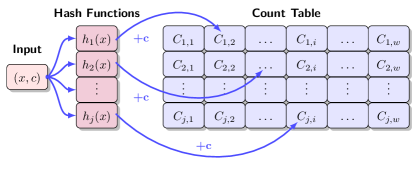
Figure 1: The update procedure for a Count-Min Sketch. It follows that $h_{j}(x)=i$.

Along with the counters $C$ and the hash functions $\{h_{i}\}$, the Count Sketch [37] has the additional collection of hash functions:

• Sign functions: $s_{1},\ldots,s_{j}:[n]\to\{-1,1\}$, which assign a random sign to each element.

For an input $X=\{x_{1},\ldots,x_{n}\}$, the update rule for Count Sketch is:

$$C(X)_{i,h_{i}(x)}\mathrel{+}=s_{i}(x),$$

for all $i\in[j]$, where $s_{i}(x)$ ensures that updates from different elements may cancel each other out. To estimate the frequency of an element $x$, Count Sketch uses the following rule:

$$\hat{f}_{x}=\text{median}\{C(X)_{i,h_{i}(x)}\cdot s_{i}(x)\mid i\in[j]\}.$$

The use of the median reduces the impact of collisions from other elements, leading to more accurate estimates.

To assess the utility of $\mathtt{PrivHP}$, we require a bound on the error in a sketch. For item $\theta$, let $c_{\theta}$ denote its exact count and $e_{\theta}$ denote the error its frequency approximation on the sketch. The expected error for the Count-Min Sketch is bound by the following result.

Lemma 4.

For all $\theta\in\Theta$, and Count-min Sketch with width $w$,

$$\mathbb{E}[e_{\theta}]\leq(n-c_{\theta})/w$$

Proof.

Each hash table in the Count-min Sketch provides a frequency estimate for each node. Let $e_{\theta}^{i}$ denote the error in the estimate of $\theta$ from the $i^{\text{th}}$ hash table. $e_{\theta}^{i}$ contains the sum of the counts of items that hash to the same entry in the $i^{\text{th}}$ hash table. Therefore,

$$e_{\theta}^{i}=\sum_{\theta^{\prime}\in\Theta\setminus\theta}\mathrm{1}[h_{i}(\theta)=h_{i}(\theta^{\prime})]\cdot c_{\theta^{\prime}}$$

Count-min Sketch selects the estimate from the hash table with the minimum error. Therefore, with the use of universal hashing [38],

$$\mathbb{E}[e_{\theta}] =\mathbb{E}[\min_{i\in[j]}e_{\theta}^{i}]$$

$$=\mathbb{E}\left[\min_{i\in[j]}\sum_{\theta^{\prime}\in\Theta\setminus\theta}\mathrm{1}[h_{i}(\theta)=h_{i}(\theta^{\prime})]\cdot c_{\theta^{\prime}}\right]$$

$$\leq\sum_{\theta^{\prime}\in\Theta\setminus\theta}\mathbb{E}[\mathrm{1}[h_{1}(\theta)=h_{1}(\theta^{\prime})]]\cdot c_{\theta^{\prime}}$$

$$=\sum_{\theta^{\prime}\in\Theta\setminus\theta}\textsf{Pr}[h_{1}(\theta)=h_{1}(\theta^{\prime})]\cdot c_{\theta^{\prime}}$$

$$\leq\sum_{\theta^{\prime}\in\Theta\setminus\theta}\frac{1}{w}\cdot c_{\theta^{\prime}}$$

$$=\frac{1}{w}\cdot(n-c_{\theta}).$$

∎

4.1 Private Release of Sketches

For private release, sketches must have similar distributions on neighboring vectors. In oblivious approaches, we sample a random vector $v\in\mathbb{R}^{j\times w}$ independent of the data and release $C(X)+v$. The sampling distribution depends on the sensitivity of the sketch. Since sketches are linear, for neighboring inputs $X\sim X^{\prime}$, we have

$$C(X)-C(X^{\prime})=C(X-X^{\prime}).$$

As neighboring inputs have sensitivity $\triangle_{1}(X-X^{\prime})=1$, a sketch $C$ has sensitivity proportional to its number of rows. Therefore, $\triangle_{1}(C)=j$ and $C(X)+v$ achieves $\varepsilon$-differential privacy for $v\sim\mathtt{Laplace}^{j\times w}(j\varepsilon^{-1})$ by Lemma 1. Pseudocode for private sketches is presented in Algorithm 1.

1 define initializeSketch$(w,j,\mathcal{D})$

2    for $i\in[j]$ do

3       Randomly select hash functions $h_{i}:\Omega\rightarrow[w]$

4       For Count Sketch randomly select hash functions $g_{i}:\Omega\rightarrow\{-1,1\}$

5      

6   Create a $j\times w$ matrix of counters $C$ initialised to $0$

7    Select random vector $v\in\mathbbm{R}^{j\times w}$ according to distribution $\mathcal{D}$

8    $C\leftarrow C+v$

9    return $C,\{h_{i}\}$ and (for Count Sketch) $\{g_{i}\}$

1 define update$(x,c)$

2    for  $i\in[j]$ do

3        $C[i][h_{i}(x)]\leftarrow\begin{cases}C[i][h_{i}(x)]+g_{i}(x)\cdot c&\text{for }\textbf{Count Sketch}\\ C[i][h_{i}(x)]+c&\text{for }\textbf{Count Min Sketch}\end{cases}$

4      

5   return

6   

1 define query$(x)$

2    return $\begin{cases}\text{median}\{g_{i}(x)\cdot C[i][h_{i}(x)]\mid i\in[j]\}&\text{for }\textbf{Count Sketch}\\ \min\{C[i][h_{i}(x)]\mid i\in[j]\}&\text{for }\textbf{Count Min Sketch}\end{cases}$

3   

Algorithm 1 Private Sketch (initialization, update, query)

5 Private, Compact Hierarchical Decomposition

A hierarchical decomposition recursively splits a sample space into smaller subdomains. Each point of splitting refers to a level in the hierarchy. Formally, for a binary partition of sample space $\Omega$, the first level of the hierarchy contains disjoint subsets $\Omega_{0},\Omega_{1}\subset\Omega$, such that $\Omega_{0}\cup\Omega_{1}=\Omega$. Thus, a hierarchical decomposition $\mathcal{T}$ of depth $r$ is a family of subsets $\Omega_{\theta}$ indexed by $\theta\in\mathcal{T}\subseteq\{0,1\}^{\leq r}$, where

$$\{0,1\}^{\leq r}:=\{0,1\}^{0}\cup\{0,1\}^{1}\cup\cdots\cup\{0,1\}^{r}.$$

By convention the cube $\{0,1\}^{0}=\varnothing$. For $\Omega_{\theta}$ with $\theta\in\{0,1\}^{l}$, we call $l$ the level of $\Omega_{\theta}$. The leaves of the decomposition $\mathcal{T}$ form a partition of the sample space. To generate synthetic data, any decomposition $\mathcal{T}$ can be used to form a sampling distribution. A synthetic point can be constructed by (1) selecting a subdomain $\Omega_{\theta}\subseteq\Omega$ with probability proportional to its cardinality and (2) conditioned on this selection, choosing a point $y\in\Omega_{\theta}$ uniformly at random.

Our lightweight generator is based on a pruned hierarchical decomposition. The quality of the generator depends on the granularity of the subsets in the partition. That is, allowing more subsets of smaller area leads to a sampling distribution closer to the empirical distribution of the input. Thus, due to the memory cost of storing a more fine-grained partition, we observe a trade-off between utility and space. To balance this trade-off, we aim to construct a hierarchical decomposition that provides finer granularity for “hot” parts of the sample space, where hot indicates a concentration of points. The high-level strategy is to branch the decomposition at hot nodes in the hierarchy. In order to bound the memory allocation, we introduce a pruning parameter $k$, which denotes the number of branches at each level of the hierarchy. Increasing $k$ allows for more branches and, thus, finer granularity at the cost of more memory.

In addition, as the space occupied by the generator is sublinear in the size of the database, we cannot rely on exact frequency counts to compute cardinalities for every possible node in the decomposition. Therefore, we employ private sketches (Algorithm 1) at deeper, and more populated, levels in the hierarchy to support approximate cardinality counting. For example, at level $l$, a single private sketch can be used to count the number of points in each subdomain $\Omega_{\theta}$, for $\theta\in\{0,1\}^{l}$. Once the private sketches process the data, they are then used to inform and grow the decomposition. That is, nodes in the hierarchy are considered hot if their noisy approximate counts are large. As the sketches are private, which means they are indistinguishable on neighboring inputs, the resulting decomposition is also private by the principle of post processing.

To describe this process in more detail, we break it down into three components: initialization; parsing the data; and growing the partition. Note that our Algorithm operates in the 1-pass streaming model. We provide information on how to adapt it to the continuous release streaming model in Appendix A.

Input: Database $\mathcal{X}$ of items from $\Omega$, pruning parameter $k$ and privacy parameters $\{\sigma_{l}\}$. Each $x\in\Omega$ has decomposition $x_{0}x_{1}\ldots x_{r}$

1 define $\mathtt{PrivHP}(\mathcal{X},(k,r),(w,j),\{\mathcal{D}_{l}\})$

2    $L_{k}\leftarrow\lfloor\log k\rfloor$

    // Initialize Data Structures

3    Initialize complete binary partition tree $\mathcal{T}$ with depth $L_{k}$

4    for $l\in\{0,\ldots,L_{k}\}$ do

5       for $v\in\{v\in\mathcal{T}\mid{\mathtt{level}}(v)=l\}$ do

6          $g\leftarrow$ random value drawn from $\mathcal{D}_{l}$

7          $v.\mathtt{count}\leftarrow g$

8         

9   for $l\in\{L_{k}+1,\ldots,r\}$ do

       $\mathtt{sketch}_{l}\leftarrow$ initialize private sketch with dimension $(w,j)$ and noise $\mathcal{D}_{l}$

        // Algorithm 1

10      

   // Parse Dataset

11    for $x\in\mathcal{X}$  do

12       for $l\in\{0,\ldots,r\}$ do

13          $\theta\leftarrow x_{0}\ldots x_{l}$

14          if $l\leq L_{k}$ then

15             Increment the counter in $v_{\theta}\in\mathcal{T}$

16            

17         else

18             $\mathtt{sketch}_{l}.\mathtt{update}(\theta)$

19            

   $\mathcal{T}_{\mathtt{PrivHP}}\leftarrow\mathtt{GrowPartition}(\mathcal{T},\{\mathtt{sketch}_{l}\},k)$

     // Algorithm 3

20    return $\mathcal{T}_{\mathtt{PrivHP}}$

21   

Algorithm 2 1-pass $\mathtt{PrivHP}$ algorithm.

5.1 Initialization

The pseudocode for initializing the component data structures is available in Algorithm 2 (Lines 2-2). The decomposition of the domain $\Omega$ is encoded in a binary tree $\mathcal{T}$, where each node in the tree $v_{\theta}\in\mathcal{T}$ represents the subset $\Omega_{\theta}$. The memory-utility trade-off for $\mathtt{PrivHP}$ is parameterized by $k$, the number of branches at each level of the decomposition. For $L_{k}=\lfloor\log k\rfloor$, the decomposition contains all subsets $\Omega_{\theta}$, for $\theta\in\{0,1\}^{\leq L_{k}}$, at levels with less than $k$ nodes. Therefore, the algorithm begins by initializing $\mathcal{T}$ as a complete binary tree of depth $L_{k}$ (Line 2).

For a decomposition of depth $r$, the sampling distribution of the generator is based on the cardinalities of each subset $\Omega_{\theta}$ for $\theta\in\{0,1\}^{\leq r}$. We store noisy exact counts for subdomains $\Omega_{\theta}$ $\{0,1\}^{\leq L_{k}}$ included in $\mathcal{T}$ and noisy approximate counts for subdomains in $\{0,1\}^{\leq r}\setminus\{0,1\}^{\leq L_{k}}$. The exact counters are stored in their corresponding nodes in $\mathcal{T}$. To ensure privacy, each counter at level $l\leq L_{k}$ is initialized with some random noise from a distribution $\mathcal{D}_{l}$ provided as input (Line 7). For each level $l>L_{k}$, the approximate counts for subsets $\Omega_{\theta}$, with $\theta\in\{0,1\}^{l}$, are stored in a private sketch ($\texttt{sketch}_{l}$) of dimension $w\times j$ and initialized with random noise from the distribution $\mathcal{D}_{l}$ (Line 2). Then, for each level $l>L_{k}$, a private sketch is initialized to store approximate counts. These sketches will be used to grow the decomposition (Line 2) according to hot subsets of the sample space once the stream has been processed.

5.2 Parsing the Data

After initialization, we read the database in a single pass, one item at a time, while updating the internal data structures $\mathcal{T}$ and $\{\mathtt{sketch}_{l}\}_{l>L_{k}}$. Each item $x\in\mathcal{X}\subseteq\Omega$ decomposes, according to the hierarchy, into a string $x_{0}x_{1}\ldots x_{r}$. Each prefix of the string names a subset in the hierarchy that contains $x$. For example, at each level $l$, it holds that $x\in\Omega_{x_{0}\ldots x_{l}}$. For each $x\in\mathcal{X}$, the procedure iterates through the levels in the hierarchy. At each level $l$, the decomposition $\theta=x_{0}\ldots x_{l}$ is observed. If $l\leq L_{k}$, then the counter in node $v_{\theta}\in\mathcal{T}$ is updated. Otherwise, $\mathtt{sketch}_{l}$ is updated with the subset index $\theta$. At the end of the stream $\mathcal{T}$ contains the noisy exact counts for subsets $\Omega_{\theta}$ with $\theta\in\{0,1\}^{\leq L_{k}}$ and the summaries $\{\mathtt{sketch}_{l}\}$ contain the noisy approximate counts for subsets at levels $l>L_{k}$. At this point, these approximate counts are used to grow $\mathcal{T}$ beyond level $L_{k}$.

Input: Partition Tree $\mathcal{T}$ and the collection of level-wise sketches $\{\mathtt{sketch}_{l}\}$

1 define $\mathtt{GrowPartition}(\mathcal{T},\{\mathtt{sketch}_{l}\},k)$

2    Apply consistency to each non-leaf node $v_{\theta}\in\mathcal{T}$ in depth-first order using Algorithm 4

3    $V\leftarrow\{\theta\mid v_{\theta}\in\mathcal{T},\mathtt{level}(v_{\theta})=L_{k}\}$

4    for $l\in\{L_{k}+1,\ldots,r-1\}$ do

5       for ${\theta}\in V$ do

6          for $\theta^{*}\in\{\theta 0,\theta 1\}$ do

7             $\hat{f}_{\theta^{*}}\leftarrow\mathtt{sketch}_{l}.\mathtt{query}(\theta^{*})$

8             add $v_{\theta^{*}}$ to $\mathcal{T}$ with $v_{\theta^{*}}.\mathtt{count}=\hat{f}_{\theta^{*}}$

9            

         Apply consistency to $v_{\theta}$

           // Algorithm 4

10         

11      $V\leftarrow$ the IDs of the Top-$k$ values in $\{v.\mathtt{count}\mid\mathtt{level}(v)=l+1\}$

12      

13   return $\mathcal{T}$

14   

Algorithm 3 Growing the $\mathtt{PrivHP}$ based on approximate counts at each level in the hierarchy.

5.3 Growing the Partition

Pseudocode for this step is available in Algorithm 3, and an illustration of the process is provided in Figure 2. Before growing the partition, a consistency step is preformed. Consistency has two objectives. First, it requires that the count of a parent node equals the sum of the counts of its child nodes. Second, it requires that all counts are non-negative. After processing the data, $\mathcal{T}$ is not consistent due to the noise added for privacy. A concrete method for consistency is presented in Section 5.4. The outcome of the consistency step is presented in Figure 2(b). A similar consistency step is common in private histograms [39], where it is observed it can increase utility at the same privacy budget.

After the consistency step has been executed, the partition is expanded one level at a time. The pseudocode is provided in Algorithm 3. It begins by selecting the current leaf nodes $V$ of $\mathcal{T}$ at level $L_{k}$ (Line 2). These are considered “hot” nodes. Then, for each hot node $v_{\theta}\in V$, it adds the two child nodes ($v_{\theta 0}$ and $v_{\theta 1}$) to $\mathcal{T}$ as the decomposition of the node into two disjoint subsets (Figure 2(c)). In addition, the nodes $v_{\theta 0}$ and $v_{\theta 1}$ are initialized with the noisy frequency estimates retrieved from $\mathtt{sketch}_{L_{k}+1}$. These estimates are then adjusted according to the consistency step (Figure 2(d)).

After all the hot nodes have been expanded, the next iteration of hot nodes needs to be selected. This is achieved by selecting the nodes with the Top-$k$ frequency estimates (Line 10). With a new set of hot nodes, this process repeats itself and stops at depth $r-1$ (Figure 2(e)). In summary, at each level in the iteration, the current hot nodes are branched into smaller subdomains at the next level in the hierarchy. Then, the new subdomains with high frequency become hot at the subsequent iteration.

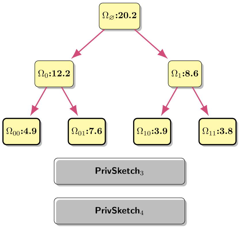
(a) After processing the stream

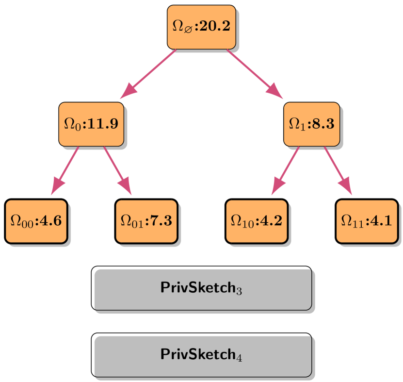
(b) After consistency is applied to the tree

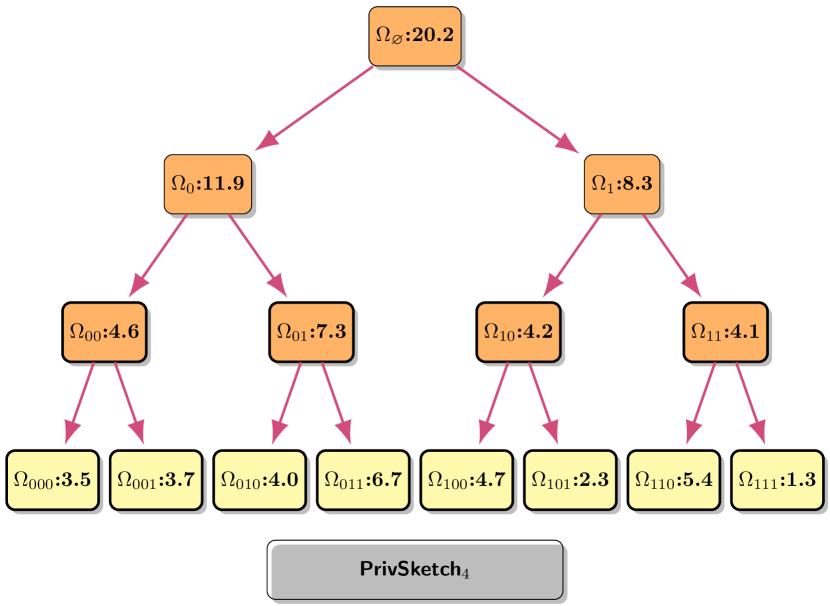
(c) Adding nodes from $\mathtt{sketch}_{3}$

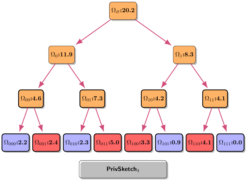
(d) After consistency is applied to level 3

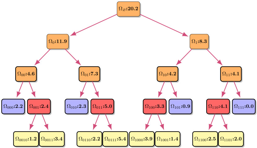
(e) Pruning based on top-$4$ selection

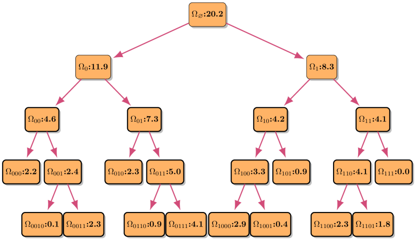
(f) After consistency is applied to level 4

Figure 2: Illustration of Algorithm 3 with $k=4$ and $r=4$. Figure 2(a) represents its input and Figure 2(f) represents its output.

5.4 Consistency

Consistency ensures that (1) all counts are non-negative and (2) that the counts of two subregions add to the count of their parent region. The consistency step in Algorithm 3 is fairly general and adheres to the following rule. In the case of a deficit, when the sum of the two subregional counts is smaller than the count of the parent region, both subregional counts should be increased. Conversely, in the case of a surplus, both subregional counts should be decreased. Apart from this requirement, we are free to distribute the deficit or surplus between the subregional counts.

Our main result (Theorem 3) relies on a concrete instance of consistency. The method we adopt is formalized in Algorithm 4. The main idea is to evenly redistribute the error generated from sibling subregions. To formalize this idea, let $v_{\theta}$ denote the parent. First, we calculate the difference between the subregional counts and their parent region (Line 4):

$$\Lambda=v_{\theta 0}.\mathtt{count}+v_{\theta 1}.\mathtt{count}-v_{\theta}.\mathtt{count}.$$

This difference is then evenly redistributed across the subregions (Line 4):

$$v_{\theta 0}.\mathtt{count}\leftarrow v_{\theta 0}.\mathtt{count}-\Lambda/2\quad\text{and}\quad v_{\theta 1}.\mathtt{count}\leftarrow v_{\theta 1}.\mathtt{count}-\Lambda/2.$$ (2)

We also add two correction steps for whenever this approach might violate consistency. The first correction makes sure that both subregional counts are non-negative prior to applying consistency (Line 4). The second involves applying a different redistribution method in the event that (2) violates consistency (Lines 4 & 4). In this instance, the count of the violating node is set to $0$ and its sibling node inherits the full count from its parent. Both correction steps reduce the amount of error in the subregion counts.

Input: Node $v_{\theta}\in\mathcal{T}$

1 define ${\mathtt{EnforceConsistency}}(v_{\theta})$

2    for $\theta^{*}\in\{\theta 0,\theta 1\}$ do

3       if $v_{\theta^{*}}.\mathtt{count}<0$  then

          // Error Correction Type 1

4          $v_{\theta^{*}}.\mathtt{count}\leftarrow 0$

5         

6   $\mathtt{sum}\leftarrow v_{\theta 0}.\mathtt{count}+v_{\theta 1}.\mathtt{count}$

7    $\Lambda\leftarrow\mathtt{sum}-v_{\theta}.\mathtt{count}$

8    if $v_{\theta 0}.\mathtt{count}-\Lambda/2<0$  then

       // Error Correction Type 2

9       $v_{\theta 0}.\mathtt{count}\leftarrow 0$

10       $v_{\theta 1}.\mathtt{count}\leftarrow v_{\theta}.\mathtt{count}$

11      

12   else if $v_{\theta 1}.\mathtt{count}-\Lambda/2<0$  then

       // Error Correction Type 2

13       $v_{\theta 1}.\mathtt{count}\leftarrow 0$

14       $v_{\theta 0}.\mathtt{count}\leftarrow v_{\theta}.\mathtt{count}$

15      

16   else

17       for $\theta^{*}\in\{\theta 0,\theta 1\}$ do

18          $v_{\theta^{*}}.\mathtt{count}\leftarrow v_{\theta^{*}}.\mathtt{count}-\Lambda/2$

19         

20   return

21   

Algorithm 4 Enforcing consistency between nodes in $\mathcal{T}$.

6 Private Synthetic Data

An item can be sampled from the decomposition tree $\mathcal{T}$ by selecting a number $u$ uniformly in the range $[0,v_{\varnothing}.\mathtt{count}]$, where $v_{\varnothing}$ is the root node of $\mathcal{T}$. Then, a root-to-leaf traversal of the tree is performed. At each node $v_{\theta}$ on the path, we retrieve the count from the left child $c\leftarrow v_{\theta 0}.\mathtt{count}$. We branch left if $c\geq u$; otherwise, we branch right. When branching right, $u$ is updated with $u\leftarrow u-v_{\theta}.\mathtt{count}$. The final leaf node represents a subset of the sample space and we can return any item uniformly at random from this subset.

Note that this sampling algorithm can take any binary decomposition of $\Omega$ as input. This makes any tree $\mathcal{T}$ synonymous with a sampling distribution. Therefore, throughout the rest of the paper we often refer to $\mathcal{T}$ as a probability distribution. Following prior work [12, 13], the utility of a decomposition can be measured by the expectation of the 1-Wasserstein distance between the empirical distribution and the distribution of the sampler. For the remainder of this section, we provide bounds on the utility of the generator $\mathcal{T}_{\mathtt{PrivHP}}$ output by Algorithm 2.

6.1 Privacy

Algorithm 3 is completely deterministic. Therefore, if the inputs to Algorithm 3 are differentially private, then the resulting partition is differentially private by the post-processing property (Lemma 2). The random perturbations introduced at initialization depend on the sequence of distributions $\{\mathcal{D}_{l}\}$. They should provide sufficient noise such that the output distributions of $\mathcal{T}$ and $\{\mathtt{sketch}_{l}\}$ on neighboring datasets are indistinguishable. The are many choices for $\{\mathcal{D}_{l}\}$ that impact both privacy and utility. Here is one example.

Theorem 2.

If the input distributions have the following form:

$$\mathcal{D}_{l} =\begin{cases}{\mathtt{Laplace}}(\sigma_{l}^{-1})&\text{for }l\leq L_{k}\\ {\mathtt{Laplace}}^{w\times j}(j\sigma_{l}^{-1})&\text{Otherwise }\end{cases}\;$$ (3)

Then, the decomposition $\mathcal{T}_{\mathtt{PrivHP}}$ output by Algorithm 2 is $\varepsilon$-differentially private for $\sum_{l=0}^{r}\sigma_{l}=\varepsilon$.

Proof.

On neighboring datasets $X=X^{\prime}\cup\{x\}$, we are required to minimize the effect of the additional element $x$ on the output distribution of the process. During data processing, the sensitive element $x$ impacts both the initial partition tree $\mathcal{T}$ and the sketches $\{\mathtt{sketch}_{l}\}$. We consider both cases separately. With $\mathcal{T}$ we store (noisy) exact counts. The sensitive element $x$ traverses a single root to leaf path, updating each node on the path, when it is processed. The counts are incremented by 1 and the path has length $L_{k}$. Therefore, the sensitivity of the initial partition tree is $L_{k}$. With noise $\mathtt{Laplace}(\sigma_{l}^{-1})$ applied to each count on the path, the initial partition tree is $\sum_{l=0}^{L_{k}}\sigma_{l}$-differentially private by Lemmas 1 &  3. As previously noted, a sketch has sensitivity $j$. Therefore, $\mathtt{Laplace}^{w\times j}(j\sigma_{l}^{-1})$ noise provides $\sigma_{l}$-differential privacy for the sketch at level $l$. Basic composition (Lemma 3) and the observation that there are $(r-L_{k})$ sketches completes the proof. ∎

6.2 Utility and Performance

Before stating our main result, we introduce some notation. Let $\gamma_{r}=\max_{\theta\in\{0,1\}^{r}}\mathtt{diam}(\Omega_{\theta})$ and

$$\Gamma_{l}=\sum_{\theta\in\{0,1\}^{l}}\mathtt{diam}(\Omega_{\theta}).$$

To help evaluate the utility of pruning, we require, for each level $l>L_{k}$, notation to capture how many points are not propagated to deeper levels (or subdomains) in the hierarchy. Let $\mathcal{C}_{l}$ denote the candidate nodes at level $l$. These nodes are output by the hot nodes at level $l-1$. We now rank the nodes in $\mathcal{C}_{l}$. Let $\theta_{l}^{(i)}\in\mathcal{C}_{l}$ denote the index for the candidate node ranked $i^{\text{th}}$ at level $l$. Therefore, $|\Omega_{\theta_{l}^{(i)}}|\geq|\Omega_{\theta_{l}^{(j)}}|$ if and only if $i\geq j$. Now, let

$$\mathtt{sum}_{l}^{i,j}=\sum_{x=i}^{j}|\Omega_{\theta_{(x)}}|$$ (4)

denote the sum of the counts from the $i^{\text{th}}$ to the $j^{\text{th}}$ candidate. Therefore, $\mathtt{sum}_{l}^{k,2k-1}$ represents the sum of the bottom-$k$ exact node counts in the candidates at level $l$.

Algorithm 2 is general and doesn’t prescribe the type of private sketch or the input distributions of the perturbations. To support an upper bound on utility, we use a private count-min sketch as the sketching primitive in Algorithm 2 and follow the input distribution of Lemma 2.

Theorem 3.

On input $\mathcal{X}$, with sketch dimensions $(w,j=1)$ and partition dimensions of depth $r$ and width $k$, for $\varepsilon=\sum_{l=0}^{r}\sigma_{l}$, Algorithm 2 produces a partition $\mathcal{T}_{\mathtt{PrivHP}}$ that is $\varepsilon$-differentially private and has the following distance from the empirical distribution $\mu_{\mathcal{X}}$ in the expected 1-Wasserstein metric:

$$\mathbb{E}[W_{1}(\mu_{\mathcal{X}},\mathcal{T}_{\mathtt{PrivHP}})] =\Delta_{\mathtt{noise}}+\Delta_{\mathtt{approx}}+\Delta_{\mathtt{resolution}},$$ (5)

where

$$\Delta_{\mathtt{noise}}=\mathcal{O}\left(\frac{1}{n}\left(\sum_{l=0}^{L_{k}}\frac{\Gamma_{l-1}}{\sigma_{l}}+\sum_{l=L_{k}+1}^{r}\frac{k\gamma_{l-1}}{\sigma_{l}}\right)\right),\quad\Delta_{\mathtt{approx}}=\mathcal{O}\left(\sum_{l=L_{k}+1}^{r}\left(\frac{1}{w}+\frac{{\mathtt{sum}}_{l}^{k,2k-1}}{n}\right)\gamma_{l-1}\right),\quad\Delta_{\mathtt{resolution}}=\mathcal{O}\left(\gamma_{r}\right)$$

Moreover, Algorithm 2 requires $\mathcal{O}((w+k)\log(\varepsilon n))$ memory, $\mathcal{O}(\log(\varepsilon n))$ update time per item and constructs the partition in $\mathcal{O}(k\log k\log\varepsilon n)$ time.

The proof of this result is the content of Section 8. The components allow us to make sense of the bound. The $\Delta_{\mathtt{noise}}$ term represents the distance incurred, between $\mu_{\mathcal{X}}$ and $\mathcal{T}_{\mathtt{PrivHP}}$, due to noise added for privacy. This noise affects both the counts and the pruning procedure. The $\Delta_{\mathtt{approx}}$ term represents the reduction in utility due to approximation. The $w^{-1}$ term is the error added due to sketching, and the sequence of $\{\mathtt{sum}_{l}^{k,2k-1}\}$ represents the error added due to pruning and reducing the number of nodes in the partition. The $\{\mathtt{sum}_{l}^{k,2k-1}\}$ terms are dependent on the underlying distribution of the input $\mathcal{X}$. It, therefore, captures the efficacy of $\mathtt{PrivHP}$ under different input distributions. Lastly, the $\Delta_{\mathtt{resolution}}$ term represents the cost of the resolution. Increasing the partition depth increases the resolution and, thus, reduces this cost.

Theorem 3 holds for generic input domain $\Omega$. In Section 9, we demonstrate the application of Theorem 1 to the hypercube $\Omega=[0,1]^{d}$. This example allows for comparison with prior work [22, 12] and also captures the asymptotics in a more concise way.

The privacy and accuracy guarantees of Theorems 2 and 3 hold for any choice of $\{\sigma_{l}\}$. By optimizing the $\{\sigma_{l}\}$, we can achieve the best utility for a given level of privacy $\varepsilon=\sum_{l=0}^{r}\sigma_{l}$.

Lemma 5.

With the optimal choice of privacy parameters (Equation (23)), on input $\mathcal{X}$ and partition dimensions of depth $r$ and width $k$, the loss in utility due to noise perturbations ($\Delta_{\mathtt{noise}}$ in (5)) is:

$$\Delta_{\mathtt{noise}}=\mathcal{O}\left(\frac{1}{\varepsilon n}\left(\sum_{l=0}^{L_{k}}\sqrt{\Gamma_{l-1}}+\sum_{l=L_{k}+1}^{r}\sqrt{k\gamma_{l-1}}\right)^{2}\right)$$

The proof is provided in Appendix B.

7 Measuring Utility

Before proving Theorem 3, we need a method to quantify the distance between $\mu_{\mathcal{X}}$ and $\mathcal{T}_{\mathtt{PrivHP}}$. In the empirical distribution, each point $x\in\mathcal{X}$ carries a unit of probability mass. When a point is abstracted into a set within a partition representing a generator, its probability mass is evenly distributed across the set. This reflects the process where, conditioned on a set being selected by the generator, a synthetic point is uniformly sampled from the set. The total distance this probability mass moves during abstraction is bounded by the diameter of the subdomain. Similarly, modifications to node counts in the decomposition tree result in shifts of probability mass within the generator. Bounding the utility of the generator, therefore, involves constraining the distance these probability masses move as $\mu_{\mathcal{X}}$ transforms into $\mathcal{T}_{\mathtt{PrivHP}}$.

To formalize these bounds, we introduce new terminology. This terminology will help account for errors arising from both noise perturbations and frequency approximations. Additionally, it will facilitate quantifying how the consistency step balances these errors across nodes. The consistency step redistributes the count of a parent node between its child nodes. Any incorrect redistribution of this count increases the distance between the empirical distribution and the synthetic data generator.

We refer to such redistribution errors as misses. The cost of a miss depends on both its magnitude and the size of the subdomain where it occurs. Thus, bounding the utility loss due to noise and approximation involves both quantifying each miss and determining where it occurs.

7.1 Quantifying a Miss

A miss represents the transfer of probability mass from one subdomain to its sibling subdomain, altering the probability distribution encoded by the underlying decomposition. To arrive at a formal evaluation of a miss, we begin by introducing some notation. Let $c_{\theta}=|\Omega_{\theta}|$ denote the exact count at node $v_{\theta}$, let $\lambda_{\theta}$ denote the noise added to $v_{\theta}.\mathtt{count}$ from privacy perturbations, and let $e_{\theta}$ denote the approximation error added to $v_{\theta}.\textsf{count}$ due to hashing collisions in the sketch. Lastly, we define $\mathtt{miss}(v_{\theta})$ as the size of a miss incurred at node $v_{\theta}$.

To help quantify $\mathtt{miss}(v_{\theta})$, we take an accounting approach, where noisy approximate counts are disaggregated into various components using the notation introduced above. This allows us to identify which part of the adjusted consistent counts constitutes a missed allocation. As we do not want to double count a miss, $\mathtt{miss}(v_{\theta})$ does not include misses that occur at ancestor nodes and are, subsequently, inherited in the count at $v_{\theta}$. Therefore, the size of $\mathtt{miss}(v_{\theta})$ is solely influenced by the errors in its two child nodes.

The size of a miss is an outcome of the method employed for consistency. The method we adopt (Algorithm 4) has the following form.

$$\Lambda=v_{\theta 0}.\mathtt{count}+v_{\theta 1}.\mathtt{count} -v_{\theta}.\mathtt{count}.$$ (6)

$$v_{\theta 0}.\mathtt{count}\leftarrow v_{\theta 0}.\mathtt{count}-\Lambda/2\quad \text{and}\quad v_{\theta 1}.\mathtt{count}\leftarrow v_{\theta 1}.\mathtt{count}-\Lambda/2.$$ (7)

Note that Algorithm 4 also contains two correction steps for when (7) might violate consistency. We will address these correction steps, and how they affect a $\mathtt{miss}$, at a later point.

For clarity, let $\mathtt{count}^{\text{before}}$ refer to a count before consistency is applied and $\mathtt{count}^{\text{after}}$ refer to a count after it is made consistent. When consistency is applied at $v_{\theta}$, consistency has already been applied to the parent of $v_{\theta}$. Therefore, the following equality already holds:

$$v_{\theta}.\mathtt{count}^{\text{after}}=c_{\theta}+\mathtt{err}_{\theta},$$ (8)

where $\mathtt{err}_{\theta}$ accumulates misses inherited at $v_{\theta}$ from its ancestors. Before consistency, the count in a child node $v_{\theta 0}$ has the following form:

$$v_{\theta 0}.\mathtt{count}^{\text{before}} =c_{\theta 0}+\lambda_{\theta 0}+e_{\theta 0}.$$

Note that $e_{\theta 0}=0$ if $\mathtt{level}(v_{\theta 0})\leq L_{k}$, as no sketches are used. To enforce consistency between child nodes, an adjustment variable (See (6)) is calculated:

$$\Lambda =v_{\theta 0}.\mathtt{count}^{\text{before}}+v_{\theta 1}.\mathtt{count}^{\text{before}}-v_{\theta}.\mathtt{count}^{\text{after}}$$

$$=c_{\theta 0}+\lambda_{\theta 0}+e_{\theta 0}+c_{\theta 1}+\lambda_{\theta 1}+e_{\theta 1}-c_{\theta}-\mathtt{err}_{\theta}$$

$$=\lambda_{\theta 0}+e_{\theta 0}+\lambda_{\theta 1}+e_{\theta 1}-\mathtt{err}_{\theta}$$

Focusing on the left child $v_{\theta 0}$, the size of a $\mathtt{miss}$ can be inferred by calculating $v_{\theta 0}.\mathtt{count}^{\text{after}}$ (See (7)).

$$v_{\theta 0}.\mathtt{count}^{\text{after}} =v_{\theta 0}.\mathtt{count}^{\text{before}}-\Lambda/2$$

$$=c_{\theta 0}+\lambda_{\theta 0}+e_{\theta 0}-(\lambda_{\theta 0}+e_{\theta 0}+\lambda_{\theta 1}+e_{\theta 1}-\mathtt{err}_{\theta})/2$$

$$=c_{\theta 0}+(\lambda_{\theta 0}-\lambda_{\theta 1}+e_{\theta 0}-e_{\theta 1})/2+\mathtt{err}_{\theta}/2$$ (9)

As $\mathtt{err}_{\theta}$ refers to points already counted as misses (which we do not wish to count twice), it follows that

$$\mathtt{miss}(v_{\theta}) =|(\lambda_{\theta 0}-\lambda_{\theta 1}+e_{\theta 0}-e_{\theta 1})/2|.$$ (10)

Therefore, a miss occurs when there is a difference in the errors in two sibling nodes. During consistency, this difference is evenly split between the subdomains. To illustrate the intuition behind this definition, we provide a detailed instance in the following Example.

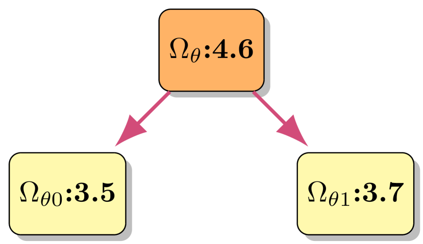
(a) Before consistency

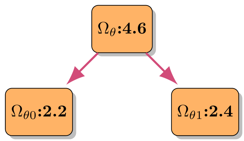
(b) After consistency

Figure 3: Subtree used for Example 7.1

With (10) in place, we can now pursue a bound for $\mathrm{E}[\mathtt{miss}(v_{\theta})]$.

Lemma 6.

With consistency applied according to Algorithm 4, on sketch parameters $w,j\in\mathbb{Z}^{+}$ and the input distribution from Equation 3, then for all internal nodes $v_{\theta}\in\mathcal{T}_{\mathtt{PrivHP}}$:

$$\mathbb{E}[|{\mathtt{miss}}(v_{\theta})|]\leq\begin{cases}2\sqrt{2}\sigma_{l+1}^{-1}&\mathtt{level}(v_{\theta})<L_{k}\\ 2\sqrt{2}\sigma_{l+1}^{-1}\cdot j+{|c_{\theta 0}-c_{\theta 1}|}{/w}&\textup{\text{Otherwise}}\end{cases}$$

Proof.

We will continue our accounting approach, disaggregating the consistent counts in child nodes into exact counts, missed counts and errors higher in the hierarchy. Depending on whether error correction is used during consistency, we have three cases to consider:

1. No error correction is used;

2. $\mathtt{Correction1}$ is used (Algorithm 4 Line 4);

3. $\mathtt{Correction2}$ is used (Algorithm 4 Lines 4 & 4).

$\mathtt{Correction1}$ and $\mathtt{Correction2}$ have the effect of reducing the amount of error in the node counts. Therefore, they cannot increase the number of misses in a node. We prove this notion formally and consider each case separately.

Case (1)

When no error correction is used, $\mathtt{miss}(v_{\theta})$ is defined in (10). Taking expectation, we get

$$\mathbb{E}[\mathtt{miss}(v_{\theta})] =\mathbb{E}[|(\lambda_{\theta 0}-\lambda_{\theta 1}+e_{\theta 0}-e_{\theta 1})/2|]$$

$$\leq\frac{1}{2}(\mathbb{E}[|\lambda_{\theta 0}-\lambda_{\theta 1}|]+\mathbb{E}[|e_{\theta 0}-e_{\theta 1}|])$$

$$\leq\mathbb{E}[\max\{|\lambda_{\theta 0}|,|\lambda_{\theta 1}|\}]+\frac{1}{2w}|c_{\theta 0}-c_{\theta 1}|$$ (11)

The third inequality follows from Lemma 4. As the $\lambda_{\theta 0}$ and $\lambda_{\theta 1}$ are independent Laplace variables with noise defined in (3), the following inequality completes the upper bound for case 1.

$$\mathbb{E}[\max\{|\lambda_{\theta 0}|,|\lambda_{\theta 1}|\}]\leq\begin{cases}2\sqrt{2}\sigma_{l}^{-1}&l\leq L_{k}\\ 2\sqrt{2}\sigma_{l}^{-1}\cdot j&\text{Otherwise}\end{cases}$$

Case (2)

We focus on a correction made to $v_{\theta 0}$. A parallel argument can be made for $v_{\theta 1}$. In $\mathtt{Correction1}$, $v_{\theta 0}.\mathtt{count}^{\text{before}}$ is set to $0$ if it is negative. As $c_{\theta 0},e_{\theta 0}\geq 0$, this can only happen if $\lambda_{\theta 0}<0$. Therefore, under our accounting approach, the correction $v_{\theta 0}.\mathtt{count}^{\text{before}}\leftarrow 0$ is made possible if $\lambda_{\theta 0}$ is changed to some value $|\lambda_{\theta 0}^{\prime}|\leq|\lambda_{\theta 0}|$. Inserting this value into Inequality (11) has the effect of reducing the bound on the number of misses.

Case (3)

As above, we focus on a correction made to $v_{\theta 0}$. A parallel argument can be made for $v_{\theta 1}$. $\mathtt{Correction2}$ is triggered on node $v_{\theta 0}$, when

$$v_{\theta 0}.\mathtt{count}^{\text{before}}-\Lambda/2<0.$$

By (9), this implies that

$$c_{\theta 0}+(\lambda_{\theta 0}-\lambda_{\theta 1})/2+(e_{\theta 0}-e_{\theta 1})/2+\mathtt{err}_{\theta}/2<0.$$ (12)

Therefore, consistency is violated when any combination of $(\lambda_{\theta 0}-\lambda_{\theta 1})$, $(e_{\theta 0}-e_{\theta 1})$ and $\mathtt{err}_{\theta}$ are non-positive and sufficiently large. The error correction step entails setting

$$v_{\theta 0}.\mathtt{count}^{\text{after}}\leftarrow 0,$$

thus, reducing the amount of error in $v_{\theta 0}.\mathtt{count}^{\text{after}}$. Following our accounting approach, this can be achieved through rescaling $\Lambda/2$ by introducing new error terms $\lambda_{\theta 0}^{\prime}$ or $e_{\theta 0}^{\prime}$, with

$$|\lambda_{\theta 0}^{\prime}-\lambda_{\theta 1}| \leq|\lambda_{\theta 0}-\lambda_{\theta 1}|$$

$$|e_{\theta 0}^{\prime}-e_{\theta 1}| \leq|e_{\theta 0}-e_{\theta 1}|,$$

such that (12) no longer holds. By inserting these values into (10), this has the effect of reducing the number of misses. Therefore, (11) holds in all three cases. ∎ This bound on the expected size of each miss is integral to the proof of the utility bound in Theorem 3.

8 Proof of Theorem 3

We break down the proof into a series of steps that are equivalent to Algorithm 2. $\mathcal{T}_{\mathtt{PrivHP}}$ can be constructed from ${\mathcal{X}}$ using the following steps:

1. Construct a partition tree $\mathcal{T}_{\mathcal{X}}$ that summarizes $\mathcal{X}$ using exact counts and a complete binary hierarchical partition of depth $r$. An example of $\mathcal{T}_{\mathcal{X}}$ is provided in Figure 4(a).

2. Conduct exact pruning on $\mathcal{T}_{\mathcal{X}}$, by keeping the nodes with the top-$k$ counts at each level, to produce $\mathcal{T}_{\mathtt{top}k}$. An example of $\mathcal{T}_{\mathtt{top}k}$ is provided in Figure 4(b).

3. Constructing $\mathcal{T}_{\mathtt{prune}}$ by adjusting $\mathcal{T}_{\mathtt{top}k}$ so that its structure matches $\mathcal{T}_{\mathtt{PrivHP}}$. $\mathcal{T}_{\mathtt{prune}}$ captures the effect of approximate pruning. Note that $\mathcal{T}_{\mathtt{prune}}$ still has exact counts. An example of $\mathcal{T}_{\mathtt{prune}}$ is provided in Figure 4(c).

4. Add the privacy noise and approximation errors to the exact counts in $\mathcal{T}_{\mathtt{prune}}$ and apply the consistency step to produce $\mathcal{T}_{\mathtt{PrivHP}}$. An example of $\mathcal{T}_{\mathtt{PrivHP}}$ is provided in Figure 4(d).

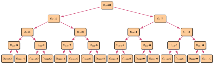
(a) Example of $\mathcal{T}_{\mathcal{X}}$. The distance between $\mu_{\mathcal{X}}$ and $\mathcal{T}_{\mathcal{X}}$ is bound in Lemma 7.

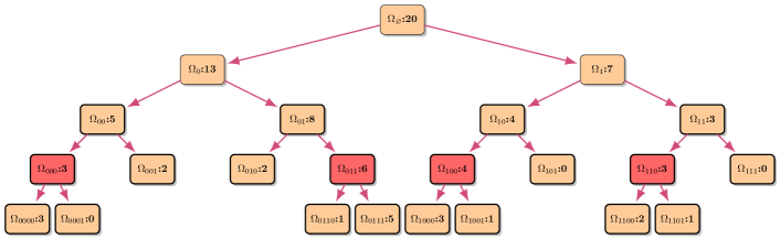
(b) Example of $\mathcal{T}_{\mathtt{top}k}$. The distance between $\mathcal{T}_{\mathcal{X}}$ and $\mathcal{T}_{\mathtt{top}k}$ is bound in Lemma 8.

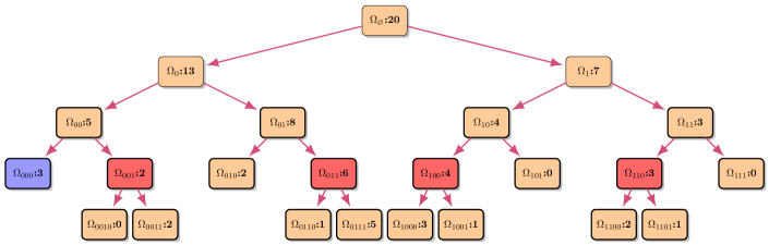
(c) Example of $\mathcal{T}_{\mathtt{prune}}$. The distance between $\mathcal{T}_{\mathtt{top}k}$ and $\mathcal{T}_{\mathtt{prune}}$ is bound in Lemma 9.

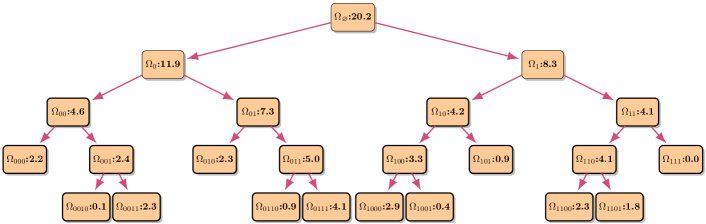
(d) Example of $\mathcal{T}_{\mathtt{PrivHP}}$. The distance between $\mathcal{T}_{\mathtt{prune}}$ and $\mathcal{T}_{\mathtt{PrivHP}}$ is bound in Lemma 10.

Figure 4: Illustration of the proof pipeline for Theorem 3.

Figure 4, illustrates the sequence of trees produced by this process. Note that these steps are equivalent to Algorithm 2. However, they are not the same and are only introduced for analytic purposes. By the triangle inequality, it follows that, to bound $\mathbb{E}[W_{1}(\mu_{\mathcal{X}},\mathcal{T}_{\mathtt{PrivHP}})]$, it suffices to bound the distance between each pair of trees in the sequence. We now bound the cost of each step separately, beginning with Step (1).

Lemma 7.

$W_{1}(\mu_{\mathcal{X}},\mathcal{T}_{\mathcal{X}}))\leq\gamma_{r}$

Proof.

A synthetic set generated from $\mathcal{T}_{\mathcal{X}}$ can be constructed by moving each point $x\in\mathcal{X}$ to a random point in the leaf node $v_{\theta}\in\mathcal{T}_{\mathcal{X}}$, where $x\in\Omega_{\theta}$. As each point moves a distance of at most $\gamma_{r}$, it follows that

$$W_{1}(\mu_{\mathcal{X}},\mathcal{T}_{\mathcal{X}})) \leq\frac{n\cdot\gamma_{r}}{n}.$$

∎

At Step (2), exact pruning has the effect of merging leaf nodes into larger subdomains. This reduces the granularity of the partition and, thus, its utility. The exact pruning step allows us to quantify the impact of the underlying data distribution on the utility of the data sampler. For example, distributions that are highly skewed will maintain a majority of the counts in the Top-$k$ nodes. Therefore, pruning will have a smaller impact on the utility of the sampler under high skew. The loss in utility is bounded by the following result (recall $\mathtt{sum}_{l}^{k,2k-1}$ defined in (4)).

Lemma 8.

$\mathbb{E}W_{1}(\mathcal{T}_{\mathcal{X}},\mathcal{T}_{\mathtt{top}k})\leq\frac{1}{n}\sum_{l=L_{k}+1}^{r-1}\gamma_{l}\mathtt{sum}_{l}^{k,2k-1}$

Proof.

The procedure to construct $\mathcal{T}_{\mathtt{top}k}$ iterates from level $L_{k}+1$ to the bottom of the tree, selecting to keep the branches with the Top-$k$ counts. Recall that $\mathcal{C}_{l}$ denotes the set of candidates at level $l$ and $\theta_{l}^{(i)}\in\mathcal{C}_{l}$ names the candidate with the $i^{\text{th}}$ largest exact cardinality. If a node $v_{\theta}$ is pruned, then each point $x\in\Omega_{\theta}\cap\mathcal{X}$ is abstracted into subdomain $\Omega_{\theta}$. This is equivalent to redistributing the probability mass of each point in $x\in\Omega_{\theta}\cap\mathcal{X}$ by moving it a distance of at most $\mathtt{diam}(\Omega_{\theta})$. As there are $2k$ candidates at each level of pruning, it follows that

$$W_{1}(\mathcal{T}_{\mathcal{X}},\mathcal{T}_{\mathtt{top}k}) \leq\frac{1}{n}\sum_{l=L_{k}+1}^{r-1}\sum_{x=k}^{2k-1}|\Omega_{\theta_{(x)}}|\cdot\mathtt{diam}(\Omega_{\theta_{(x)}})$$

$$\leq\frac{1}{n}\sum_{l=L_{k}+1}^{r-1}\gamma_{l}\sum_{x=k}^{2k-1}|\Omega_{\theta_{(x)}}|$$

$$=\frac{1}{n}\sum_{l=L_{k}+1}^{r-1}\gamma_{l}\mathtt{sum}_{l}^{k,2k-1}.$$

∎

With approximate pruning, each miss propagates down the tree and affects future pruning decisions. The main challenge in the proof of the bound for Step (3) involves demonstrating that the influence of each miss decays as it propagates down the tree. The following result bounds the utility loss at Step (3).

Lemma 9.

$\mathbb{E}W_{1}(\mathcal{T}_{\mathtt{top}k},\mathcal{T}_{\mathtt{prune}})\lesssim\frac{4}{n}\left(\sum_{l=1}^{L_{k}}2\sqrt{2}\sigma_{l}^{-1}\Gamma_{l-1}+\sum_{l=L_{k}+1}^{r}(2\sqrt{2}j\sigma_{l}^{-1}k+n/w)\gamma_{l-1}\right)$

Proof.

At Step (3), we adjust the tree structure to reflect the impact of noisy approximate pruning (Figure 4(c)). Nodes can “jump” into the top-$k$ due to the effect of misses. We refer to the size of a jump as the difference in exact counts between the jumping node and the true top-$k$ node it displaces. A jump of size $c$ occurs, for some $\theta_{1},\theta_{2}\in\{0,1\}^{l}$, with $l>L_{k}$, under the following conditions:

• $v_{\theta_{1}}.\mathtt{count}>v_{\theta_{2}}.\mathtt{count}$;

• $|\Omega_{\theta_{1}}|+c=|\Omega_{\theta_{2}}|$ for integer constant $c>0$;

• and, when $v_{\theta_{2}}$ is in the exact top-$k$ and $v_{\theta_{1}}$ is not in the exact top-$k$.

The cost of each jump is at most $c\cdot\gamma_{l}$, representing $c$ additional points that are abstracted into a subdomain at level $l$. Therefore, the distance between the sampling distributions defined by $\mathcal{T}_{\mathtt{top}k}$ and $\mathcal{T}_{\mathtt{prune}}$ is determined by the size of the jumps that occur due to approximate pruning. Further, the size of a jump at a given level is determined by misses that are inherited from ancestor nodes.

A miss can propagate through hot nodes and influence multiple levels of pruning. To demonstrate this phenomenon formally, let $\mathtt{cost}_{l}(v_{\theta})$ denote the cost incurred by $\mathtt{miss}(v_{\theta})$ during pruning at level $l$. We first consider $v_{\theta}$ with $\mathtt{level}(v_{\theta})=l_{\theta}\geq L_{k}$. The error $\mathtt{miss}(v_{\theta})$ is passed to both candidate subdomains $v_{\theta 0}$ and $v_{\theta 1}$. One subdomain will receive $\mathtt{miss}(v_{\theta})$ as an addition, allowing it to jump upwards, and the other subdomain will receive $\mathtt{miss}(v_{\theta})$ as a subtraction, allowing it to jump downwards. Therefore, the cost incurred by $\mathtt{miss}(v_{\theta})$ at level $l_{\theta}+1$ is

$$\mathtt{cost}_{l_{\theta}+1}(v_{\theta}) \leq\mathtt{miss}(v_{\theta})\cdot\gamma_{l_{\theta}+1}+\mathtt{miss}(v_{\theta})\cdot\gamma_{l_{\theta}+1}=2\mathtt{miss}(v_{\theta})\cdot\gamma_{l_{\theta}+1}.$$

If these subdomains are hot, then, due to consistency, $\mathtt{miss}(v_{\theta})$ is evenly redistributed during the branching process. Thus, all of $v_{\theta 00},v_{\theta 01},v_{\theta 10},v_{\theta 10}$ contain (as either an addition or subtraction) $\mathtt{miss}(v_{\theta})/2$ in their counts. If either subdomain is cold, then its portion of $\mathtt{miss}(v_{\theta})$ ceases to participate in pruning. Assuming the worst-case, where both subdomains are hot,

$$\mathtt{cost}_{l_{\theta}+2}(v_{\theta}) \leq 4\cdot\frac{\mathtt{miss}(v_{\theta})}{2}\gamma_{l_{\theta}+2}=2\mathtt{miss}(v_{\theta})\cdot\gamma_{l_{\theta}+2}\approx\mathtt{miss}(v_{\theta})\cdot\gamma_{l_{\theta}+1},$$

as $2\gamma_{l}\approx\gamma_{l-1}$. Repeating this process, assuming, in the worst-case, that all subdomains are hot and continue to propagate $\mathtt{miss}(v_{\theta})$, it follows that

$$\mathtt{cost}_{l_{\theta}+x}(v_{\theta}) \leq\max\{2^{x},k\}\cdot\frac{\mathtt{miss}(v_{\theta})}{2^{x-1}}\gamma_{l_{\theta}+x}\leq 2\mathtt{miss}(v_{\theta})\cdot\gamma_{l_{\theta}+x}\approx 2\mathtt{miss}(v_{\theta})\cdot\frac{\gamma_{l_{\theta}+1}}{2^{x-1}},$$

Accumulating these costs, we get

$$\sum_{x<(r-l_{\theta}-1)}\mathtt{cost}_{l_{\theta}+x}(v_{\theta}) \lesssim 4\mathtt{miss}(v_{\theta})\cdot\gamma_{l_{\theta}+1}.$$

This applies to nodes $v_{\theta}$ at levels $l_{\theta}\geq L_{k}$. The same analysis extends to nodes $v_{\theta}$ at levels $l_{\theta}<L_{k}$, except that the first level of pruning $\mathtt{miss}(v_{\theta})$ participates in is $L_{k}+1$ (not $l_{\theta}+1$). Adding everything together, we arrive at the following bound for the distance between $\mathcal{T}_{\mathtt{top}k}$ and $\mathcal{T}_{\mathtt{prune}}$.

$$W_{1}(\mathcal{T}_{\mathtt{top}k},\mathcal{T}_{\mathtt{prune}})) \lesssim\sum_{l=0}^{L_{k}-1}\sum_{\theta:\mathtt{level}(\theta)=l}4\mathtt{miss}(v_{\theta})\cdot\gamma_{L_{k}+1}+\sum_{l=L_{k}}^{r-1}\sum_{v_{\theta}\in\mathcal{H}_{l}}4\mathtt{miss}(v_{\theta})\cdot\gamma_{l+1}$$

$$\leq\sum_{l=0}^{L_{k}-1}\sum_{\theta:\mathtt{level}(\theta)=l}4\mathtt{miss}(v_{\theta})\cdot\mathtt{diam}(\Omega_{\theta})+\sum_{l=L_{k}}^{r-1}\sum_{v_{\theta}\in\mathcal{H}_{l}}4\mathtt{miss}(v_{\theta})\cdot\gamma_{l+1}$$

Taking expectations, and using Lemma 6, we arrive at the following.

$$\mathbb{E}[W_{1}(\mathcal{T}_{\mathtt{top}k},\mathcal{T}_{\mathtt{prune}})] \lesssim\frac{4}{n}\left(\sum_{l=0}^{L_{k}-1}\sum_{\theta:\mathtt{level}(\theta)=l}\mathbb{E}[\mathtt{miss}(v_{\theta})]\cdot\mathtt{diam}(\Omega_{\theta})+\sum_{l=L_{k}}^{r-1}\sum_{v_{\theta}\in\mathcal{H}_{l}}\mathbb{E}[\mathtt{miss}(v_{\theta})]\cdot\gamma_{l+1}\right)$$

$$\leq\frac{4}{n}\left(\sum_{l=0}^{L_{k}-1}2\sqrt{2}\sigma_{l+1}^{-1}\sum_{\theta:\mathtt{level}(\theta)=l}\mathtt{diam}(\Omega_{\theta})+\sum_{l=L_{k}}^{r-1}\gamma_{l}\sum_{v_{\theta}\in\mathcal{H}_{l}}2\sqrt{2}\sigma_{l+1}^{-1}j+|c_{\theta 0}-c_{\theta 1}|/w\right)$$

$$\leq\frac{4}{n}\left(\sum_{l=0}^{L_{k}-1}2\sqrt{2}\sigma_{l+1}^{-1}\Gamma_{l}+\sum_{l=L_{k}}^{r-1}\gamma_{l}\sum_{v_{\theta}\in\mathcal{H}_{l}}2\sqrt{2}\sigma_{l+1}^{-1}j+c_{\theta}/w\right)$$

$$=\frac{4}{n}\left(\sum_{l=0}^{L_{k}-1}2\sqrt{2}\sigma_{l+1}^{-1}\Gamma_{l}+\sum_{l=L_{k}}^{r-1}\gamma_{l}\left(\left(2\sqrt{2}\sigma_{l+1}^{-1}j\sum_{v_{\theta}\in\mathcal{H}_{l}}\right)+\frac{\sum_{v_{\theta}\in\mathcal{H}_{l}}c_{\theta}}{w}\right)\right)$$

$$\leq\frac{4}{n}\left(\sum_{l=1}^{L_{k}}\frac{2\sqrt{2}\Gamma_{l-1}}{\sigma_{l}}+\sum_{l=L_{k}+1}^{r}\left(\frac{2\sqrt{2}jk}{\sigma_{l}}+\frac{n}{w}\right)\gamma_{l-1}\right)$$ (13)

∎

Step (3) quantifies how the consistency step affects pruning decisions. $\mathcal{T}_{\mathtt{prune}}$ has the same structure as $\mathcal{T}_{\mathtt{PrivHP}}$, but not the same counts. Step (4) introduces these (noisy and approximate) counts and, therefore, accounts for the utility loss incurred due to errors in the sampling probabilities.

Lemma 10.

$\mathbb{E}W_{1}(\mathcal{T}_{\mathtt{prune}},\mathcal{T}_{\mathtt{PrivHP}})\leq\frac{1}{n}\left(\sum_{l=0}^{L_{k}}2\sqrt{2}\sigma_{l}^{-1}\Gamma_{l-1}+\sum_{l=L_{k}+1}^{r}(2\sqrt{2}j\sigma_{l}^{-1}k+n/w)\gamma_{l-1}\right)$

Due to its similarity to the proof of Theorem 10 in He et al. [12], the proof is placed in Appendix C. With a bound on the cost of each step in the proof pipeline, we can proceed with the proof of Theorem 3.

Proof of Theorem 3.

By the triangle inequality, the following holds

$$\mathbb{E}[W_{1}(\mu_{\mathcal{X}},\mathcal{T}_{\mathtt{PrivHP}})] \leq\mathbb{E}[W_{1}(\mu_{\mathcal{X}},\mathcal{T}_{\mathcal{X}})]+\mathbb{E}[W_{1}(\mathcal{T}_{\mathcal{X}},\mathcal{T}_{\mathtt{top}k})]+\mathbb{E}[W_{1}(\mathcal{T}_{\mathtt{top}k},\mathcal{T}_{\mathtt{prune}})]+\mathbb{E}[W_{1}(\mathcal{T}_{\mathtt{prune}},\mathcal{T}_{\mathtt{PrivHP}})]$$

By Lemmas 7, 8, 9, and 10, this evaluates as

$$\mathbb{E}[W_{1}(\mu_{\mathcal{X}},\mathcal{T}_{\mathtt{PrivHP}})] \lesssim\frac{1}{n}\left(\sum_{l=0}^{L_{k}}10\sqrt{2}\sigma_{l}\Gamma_{l-1}+\sum_{l=L_{k}+1}^{r}(10\sqrt{2}\sigma_{l}jk+5n/w)\gamma_{l-1}+\sum_{l=L_{k}+1}^{r-1}\gamma_{l}\mathtt{sum}_{l}^{k,2k-1}\right)+\gamma_{r}.$$

$$\lesssim\frac{10\sqrt{2}}{n}\left(\sum_{l=0}^{L_{k}}\frac{\Gamma_{l-1}}{\sigma_{l}}+\sum_{l=L_{k}+1}^{r}\frac{k\gamma_{l-1}}{\sigma_{l}}\right)+\sum_{l=L_{k}+1}^{r}\left(\frac{5}{w}+\frac{\mathtt{sum}_{l}^{k,2k-1}}{n}\right)\gamma_{l-1}+\gamma_{r}$$

For the memory bound, we need to account for both the tree and the sketches. The tree has $r$ levels, each with at most $k$ nodes. Therefore, the tree occupies $\mathcal{O}(kr)$ words of memory. There are $r-\log k=\mathcal{O}(\log\varepsilon n)$ sketches. Each sketch occupies $w\cdot j=\mathcal{O}(w)$ words of memory, for $j=\mathcal{O}(1)$. Therefore, $\mathtt{PrivHP}$, comprising the partition tree and the sketches, occupies $\mathcal{O}((w+k)\log\varepsilon n)$ words of memory. At each update, $x\in\mathcal{X}$ performs a root to leaf traversal, updating the counter for each node. Both exact and approximate counters are updated in constant time. Therefore the cost of an update is $\mathcal{O}(r)=\mathcal{O}(\log(\varepsilon n)$.

The partition tree is built one level at a time. Each level has $k$ nodes. The noisy frequency estimates for each node can each be retrieved in $\mathcal{O}(1)$ time. Once the estimates are retrieved, they need to be sorted so that the bottom-$k$ can be pruned. Sorting takes $\mathcal{O}(k\log k)$ time. There are $\mathcal{O}(r-L_{k})=\mathcal{O}(\log\varepsilon n)$ levels that are grown on the partition tree. Therefore, it takes $\mathcal{O}(k\log k\log\varepsilon n)$ time to grow the partition tree. Further, consistency requires $\mathcal{O}(1)$ time per node. There are at most $\mathcal{O}(kr)=\mathcal{O}(k\log\varepsilon n)$ nodes. Therefore, the time required to perform consistency is negligible. ∎

9 Synthetic Data on the Hypercube

Theorem 3 applies for any input domain $\Omega$. To make the result more tangible and to demonstrate its applicability, following prior work [22, 12], we apply it (in conjunction with Lemma 5) to the hypercube $\Omega=[0,1]^{d}$. This leads to the following result.

Corollary 1.

When $\Omega=[0,1]^{d}$ equipped with the $l^{\infty}$ metric, for sketch parameter $w$ and pruning parameter $k$, $\mathtt{PrivHP}$ can process a stream $\mathcal{X}$ of size $n$ in $\mathcal{O}((w+k)\log(\varepsilon n))$ memory and $\mathcal{O}(\log(\varepsilon n))$ update time. $\mathtt{PrivHP}$ can subsequently output a $\varepsilon$-differentially private synthetic data generator $\mathcal{T}_{\mathtt{PrivHP}}$, in $\mathcal{O}(k\log k\log\varepsilon n)$ time, such that

$$\mathbb{E}[W_{1}(\mu_{\mathcal{X}},\mathcal{T}_{\mathtt{PrivHP}})]=\begin{cases}\mathcal{O}\left(\frac{\log^{2}(k)}{\varepsilon n}+k^{-1}(w^{-1}+f(\mathcal{X},k))\right)&ifd=1\\ \mathcal{O}\left(\frac{k^{(1-\frac{1}{d})}}{\varepsilon n}+{k^{-\frac{1}{d}}}(w^{-1}+f(\mathcal{X},k))\right)&ifd\geq 2\end{cases},$$

where $f$ is a function that depends only on the input dataset and $k$. Moreover,

$$f(\mathcal{X},k) =\begin{cases}\mathcal{O}(1)&if\mathcal{X}\sim\mathtt{Uniform}([0,1]^{d})\\ \mathcal{O}(1-B)&if\mathcal{X}\sim\mathtt{MultiFractal}(B,[0,1]^{d})\end{cases}$$

We can employ this theorem to evaluate utility bounds under specific values of $k$ and $w$. For example, in streaming settings, it is standard to utilize a data structure that has memory polylogarithmic in the size of the stream. Therefore, setting $k,w\in\mathtt{poly}\log(n)$, we observe a polylogarithmic memory allocation that is inversely proportional to utility. In addition, Corollary 1 demonstrates that the utility of our generator improves when there is more skew (that is, when $B$ increases) in the stream.

For comparison, for $d=1$, $\mathtt{PMM}$ achieves a utility bound of $\mathcal{O}(\log^{2}(\varepsilon n)(\varepsilon n)^{-1})$ in a memory cost that is $\mathcal{O}(\varepsilon n)$ (Table 1). Our method is identical to $\mathtt{PMM}$ for $k=n$. Therefore, the second term in our bound, $k^{-1}(w^{-1}+f(\mathcal{X},k))$, quantifies the cost introduced by moving to a smaller memory solution. Either increasing the size of the sketches $w$, supporting more accurate frequency estimates, or increasing the pruning parameter $k$, supporting a larger partition of the sample space, enables improved utility at the cost of more memory.

Before presenting the proof of Corollary 1, we require additional results to account for the input distributions ($\mathcal{X}\sim\mathtt{Uniform}$ and $\mathcal{X}\sim\mathtt{MultiFractal}$) and the input domain ($\Omega=[0,1]^{d}$). These are provided in the following subsection.

9.1 Supporting Lemmas

The influence of the input distribution on utility is expressed by the $\mathtt{sum}_{l}^{k,2k-1}$ term in Theorem 3. The following result evaluates this term when the input is distributed according to the $\mathtt{Uniform}$ and $\mathtt{MultiFractal}$ distributions. An overview of the $\mathtt{MultiFractal}$ distribution is provided in Section 3.3.

Lemma 11.

With pruning parameter $k$, on input $\mathcal{X}$, the following holds $\forall l>L_{k}$

$$\mathbb{E}[\mathtt{sum}_{l}^{k,2k-1}] \leq\begin{cases}\frac{1}{2^{l-L_{k}}}\cdot n&\mathcal{X}\sim\mathtt{Uniform}(\Omega)\\ (1-B)B^{l-(L_{k}+1)}\cdot n&\mathcal{X}\sim\mathtt{MultiFractal}(B,\Omega)\end{cases}$$

Proof.

Starting with $\mathcal{X}\sim\mathtt{Uniform}(\Omega)$, at each level $l>L_{k}$, we prune half of the remaining branches. As items are distributed uniformly across the subsets in expectation, at the first level of pruning $\mathbb{E}[\mathtt{sum}^{k,2k-1}_{L_{k}+1}]=n/2$. At the subsequent level $n/2$ items remain and half of the branches are pruned. Therefore,

$$\mathbb{E}[\mathtt{sum}^{k,2k-1}_{L_{k}+2}] =n/2-1/2\cdot n/2=n/4.$$

Repeating in this way for $l>L_{k}+2$, we get

$$\mathbb{E}[\mathtt{sum}^{k,2k-1}_{l}]=\frac{1}{2^{l-L_{k}}}\cdot n.$$

For $\mathcal{X}\sim\mathtt{MultiFractal}(B,\Omega)$, the input data exhibits skew modeled by the parameter $B$: at a given node $v_{\theta}$, in expectation, a $B$ portion of the data belongs to the left subdomain, and a $1-B$ portion of the data belongs to the right subdomain. Let $\mathcal{C}_{l}$ denote the set of hot nodes at level $l\geq L_{k}$. The children of the nodes in $\mathcal{H}_{l}$ constitute the candidates at level $l+1$. As an upper bound on $\mathtt{sum}_{l+1}^{k,2k-1}$ we can select all the right branching children generated from $\mathcal{H}_{l}$

$$\mathbb{E}[\mathtt{sum}_{l+1}^{k,2k-1}]\leq(1-B)\sum_{\theta\in\mathcal{H}_{l}}|\Omega_{\theta}|.$$

By the reverse argument, we can lower bound the sum of the top-$k$ nodes $\mathtt{sum}_{l+1}^{0,k-1}$

$$\mathbb{E}[\mathtt{sum}_{l+1}^{0,k-1}]\geq B\sum_{\theta\in\mathcal{H}_{l}}|\Omega_{\theta}|.$$

Therefore, the ratio of the two sums is bounded above as

$$\frac{\mathbb{E}[\mathtt{sum}_{l+1}^{k,2k-1}]}{\mathbb{E}[\mathtt{sum}_{l+1}^{0,k-1}]} \leq\frac{1-B}{B}.$$

This ratio implies that, at most, a $(1-B)$ portion of $\sum_{\theta\in\mathcal{H}_{l}}|\Omega_{\theta}|$ is transferred to the pruned nodes. Therefore, at the first level of pruning,

$$\mathbb{E}[\mathtt{sum}_{L_{k}+1}^{k,2k-1}] \leq(1-B)n.$$

Iterating down the hierarchy, as $\sum_{\theta\in\mathcal{H}_{L_{k}+1}}|\Omega_{\theta}|\geq B\cdot n$, it follows that, at the second level of pruning,

$$\mathbb{E}[\mathtt{sum}_{L_{k}+2}^{k,2k-1}] \leq(1-B)Bn.$$

Repeating this process, we get, for $l>L_{k}$,

$$\mathbb{E}[\mathtt{sum}_{l}^{k,2k-1}] \leq(1-B)B^{l-(L_{k}+1)}n.$$

∎

We now move our attention to the hypercube $\Omega=[0,1]^{d}$, which is the domain of Corollary 1. The following Lemma bounds the sum of the hypercube subdomain diameters across the pruned levels.

Lemma 12.

On input domain $\Omega=[0,1]^{d}$, $d\in\mathrm{Z}^{+}$, privacy budget $\varepsilon>0$, and hierarchy depth $r=\log\varepsilon n$,

$${\sum_{l=L_{k}+1}^{r}}\gamma_{l-1} =\mathcal{O}(k^{-1/d}).$$

Proof.

Recall that $L_{k}=\log k$. Let $\Omega=[0,1]$ equipped with the $l_{\infty}$ metric. The natural hierarchical binary decomposition of $[0,1]$ (cut through the middle) makes sub-intervals of length $\mathtt{diam}(\Omega_{\theta})=\gamma_{l}=2^{-l}$ for $\theta\in\{0,1\}^{l}$. Therefore, it follows that

$$\sum_{l={L_{k}+1}}^{r}\gamma_{l-1} =\sum_{l=L_{k}}^{r-1}2^{-l}=\mathcal{O}(2^{-L_{k}})=\mathcal{O}(k^{-1}).$$

Generalizing to $\Omega=[0,1]^{d}$, the natural hierarchical binary decomposition of $[0,1]^{d}$ (cut through the middle along a coordinate hyperplane) makes subintervals of length $\mathtt{diam}(\Omega_{\theta})=\gamma_{l}\asymp 2^{-l/d}$, for $\theta\in\{0,1\}^{l}$. Note that $\sum_{l={L_{k}+1}}^{r}\gamma_{l-1}=\sum_{l=\log k}^{\log(\varepsilon n)-1}2^{-l/d}$ is a finite geometric series with common ratio $\rho=2^{-1/d}$. Therefore, we can rewrite the sum using the following formula.

$$\sum_{l=a}^{b}\rho^{l}=\frac{\rho^{a}(1-\rho^{b-a+1})}{1-\rho},$$ (14)

where $b=\log(\varepsilon n)-1$ and $a=\log k$. Therefore, we get

$$\sum_{l=\log k}^{\log(\varepsilon n)-1}2^{-l/d} =2^{-(\log k)/d}\cdot\frac{1-2^{-(\log\varepsilon n-\log k)/d}}{1-2^{-1/d}}$$

$$=k^{-1/d}\cdot\frac{1-\left(\frac{k}{\varepsilon n}\right)^{1/d}}{1-2^{-1/d}}$$

To evaluate the asymptotics of $\frac{1-\left(\frac{k}{\varepsilon n}\right)^{1/d}}{1-2^{-1/d}}$, we look at its behavior as $d$ and $n$ increase. Clearly, this fraction approaches a constant (for fixed $d$) as $n\rightarrow\infty$. To determine whether this constant depends on $d$, we need to determine the behavior of the fraction when $d\rightarrow\infty$. Both the numerator and the denominator approach $0$ as $d$ increases. Therefore, we apply L’Hopital’s rule to find the limit. Differentiating the numerator, we get

$$\frac{d}{dd}\left(1-\left(\frac{k}{\varepsilon n}\right)^{1/d}\right) =\frac{\ln\left(\frac{k}{\varepsilon n}\right)\cdot\left(\frac{k}{\varepsilon n}\right)^{1/d}}{d^{2}}.$$ (15)

Differentiating the denominator, we get

$$\frac{d}{dd}(1-2^{-1/d})=-\frac{\ln 2\cdot 2^{-1/d}}{d^{2}}$$ (16)

Combining (15) and (16) with L’Hopital’s rule, we get

$$\lim_{d\rightarrow\infty}\frac{1-\left(\frac{k}{\varepsilon n}\right)^{1/d}}{1-2^{-1/d}} =\lim_{d\rightarrow\infty}-\frac{\ln\left(\frac{k}{\varepsilon n}\right)\cdot\left(\frac{k}{\varepsilon n}\right)^{1/d}}{\ln 2\cdot 2^{-1/d}}$$

$$=-\frac{\ln\left(\frac{k}{\varepsilon n}\right)}{\ln 2}$$

This is a constant for fixed $n$. The fraction approaches a constant as either $d$ or $n$ approaches infinity. Therefore, for all values of $d$ and $n$, $\frac{1-\left(\frac{k}{\varepsilon n}\right)^{1/d}}{1-2^{-1/d}}$ is bound above by some value $C\geq 0$. ∎

9.2 Proof of Corollary 1

With these Lemmas in place, we are ready to proceed with the Proof of Corollary 1. Recall that Corollary 1 is an extension of Theorem 3 on the hypercube. We begin by restating the result.

See 1

Proof.

The memory allocation and construction time directly follow from Theorem 3. Let $\Omega=[0,1]$ equipped with the $l_{\infty}$ metric. The natural hierarchical binary decomposition of $[0,1]$ makes sub-intervals of length $\mathtt{diam}(\Omega_{\theta})=\gamma_{l}=2^{-l}$ for $\theta\in\{0,1\}^{l}$. Therefore, $\Gamma_{l}=1$. Extending Theorem 3 to $\Omega=[0,1]$, we proceed by bounding the noise, approximation and resolution terms separately. Starting with the noise term $\Delta_{\mathtt{noise}}$, and noting that, for $l>L_{K}$, $k\gamma_{l}=2^{-(l-L_{k}-1)}$, by Lemma 5 the following holds for some constant $C_{1}\geq 0$.

$$\Delta_{\mathtt{noise}}\leq\frac{C_{1}}{\varepsilon n}\left(\sum_{l=0}^{L_{k}}\sqrt{\Gamma_{l-1}}+\sum_{l=L_{k}+1}^{r}\sqrt{k\gamma_{l-1}}\right)^{2} =\frac{C_{1}}{\varepsilon n}\left(\sum_{l=0}^{L_{k}}+\sum_{l=L_{k}+1}^{\log(\varepsilon n)}\sqrt{2^{-(l-L_{k}-1)}}\right)^{2}$$

$$=\frac{C_{1}}{\varepsilon n}\left(\log(k)+\mathcal{O}(1)\right)^{2}$$

$$=\mathcal{O}(\log^{2}(k)/(\varepsilon n))$$ (17)

The approximation term utilizes Lemma 12, for sufficiently large constant $C_{2}\geq 0$

$$\Delta_{\mathtt{approx}}\leq C_{2}\sum_{l=L_{k}+1}^{r}\left(\frac{1}{w}+\frac{\mathtt{sum}_{l}^{k,2k-1}}{n}\right)\gamma_{l-1} \leq C_{2}\left(\frac{1}{w}+\max_{l>L_{k}}\frac{\mathtt{sum}_{l}^{k,2k-1}}{n}\right)\sum_{l=L_{k}+1}^{r}\gamma_{l-1}$$

$$=\mathcal{O}(k^{-1}(w^{-1}+f(\mathcal{X},k))),$$ (18)

where $f(\mathcal{X},k)=\max_{l>L_{k}}\mathtt{sum}_{l}^{k,2k-1}/n$. Lastly, the resolution term is evaluated as

$$\Delta_{\mathtt{resolution}}=\mathcal{O}(\gamma_{r})=\mathcal{O}(2^{-r}) =\mathcal{O}\left((\varepsilon n)^{-1}\right)$$ (19)

Combining (17), (18) and (19), for $\Omega=[0,1]$, we get:

$$\mathbb{E}[W_{1}(\mu_{\mathcal{X}},\mathcal{T}_{\mathtt{PrivHP}})] =\Delta_{\mathtt{noise}}+\Delta_{\mathtt{approx}}+\Delta_{\mathtt{resolution}}$$

$$=\mathcal{O}\left(\frac{\log^{2}(k)}{\varepsilon n}\right)+\mathcal{O}\left(\frac{1}{k}\left(\frac{1}{w}+f(\mathcal{X},k)\right)\right)+\mathcal{O}\left((\varepsilon n)^{-1}\right)$$

$$=\mathcal{O}\left(\frac{\log^{2}(k)}{\varepsilon n}+\frac{1}{k}\left(\frac{1}{w}+f(\mathcal{X},k)\right)\right)$$

Let $\Omega=[0,1]^{d}$. The natural hierarchical binary decomposition of $[0,1]^{d}$ makes subintervals of length $\mathtt{diam}(\Omega_{\theta})=\gamma_{l}\asymp 2^{-l/d}$, for $\theta\in\{0,1\}^{l}$. Therefore, $\Gamma_{l}=2^{l}\cdot 2^{-l/d}=2^{(1-1/d)l}$. We follow the same procedure as above, bounding each term in Theorem 3 separately. By Lemma 5,

$$\Delta_{\mathtt{noise}}\leq\frac{C_{1}}{\varepsilon n}\left(\sum_{l=0}^{L_{k}}\sqrt{\Gamma_{l-1}}+\sum_{l=L_{k}+1}^{r}\sqrt{k\gamma_{l-1}}\right)^{2} =\frac{C_{1}}{\varepsilon n}\left(\sum_{l=0}^{L_{k}}\sqrt{2^{(1-1/d)l}}+\sum_{l=L_{k}+1}^{r}\sqrt{k2^{-l/d}}\right)^{2}$$

$$=\frac{C_{1}}{\varepsilon n}\left(\mathcal{O}\left(2^{\frac{1}{2}(1-\frac{1}{d})L_{k}}\right)+k^{1/2}\sum_{l=L_{k}+1}^{r}2^{-l/(2d)}\right)^{2}$$

$$=\mathcal{O}\left(\frac{(k^{(1-\frac{1}{d})/2}+k^{1/2}k^{-1/(2d)})^{2}}{\varepsilon n}\right)$$

$$=\mathcal{O}\left(\frac{k^{(1-\frac{1}{d})}}{\varepsilon n}\right)$$ (20)

The third line comes from Lemma 12, by setting the dimension to $2d$. As in the $\Omega=[0,1]$ case, the approximation term for $\Omega=[0,1]^{d}$ utilizes Lemma 12.

$$\Delta_{\mathtt{approx}}\leq C_{2}\sum_{l=L_{k}+1}^{r}\left(\frac{1}{w}+\frac{\mathtt{sum}_{l}^{k,2k-1}}{n}\right)\gamma_{l-1} \leq C_{2}\left(\frac{1}{w}+\max_{l>L_{k}}\mathtt{sum}_{l}^{k,2k-1}\right)\sum_{l=L_{k}+1}^{r}\gamma_{l-1}$$

$$=\mathcal{O}(k^{-1/d}(w^{-1}+f(\mathcal{X},k))$$ (21)

Lastly, the resolution term is

$$\Delta_{\mathtt{resolution}}=\gamma_{r} \leq 2^{-r/d}=(\varepsilon n)^{-1/d}.$$ (22)

Combining (20), (21) and (22), for $\Omega=[0,1]^{d}$, we get

$$\mathbb{E}[W_{1}(\mu_{\mathcal{X}},\mathcal{T}_{\mathtt{PrivHP}})]=\Delta_{\mathtt{noise}}+\Delta_{\mathtt{approx}}+\Delta_{\mathtt{resolution}} =\mathcal{O}\left(\frac{k^{(1-\frac{1}{d})}}{\varepsilon n}+k^{-1/d}(w^{-1}+f(\mathcal{X},k))\right)$$

Lastly, to complete the proof, by Lemma 11

$$f(\mathcal{X},k) =\max_{l>L_{k}}\frac{\mathtt{sum}_{l}^{k,2k-1}}{n}=\begin{cases}\mathcal{O}(1)&\mathcal{X}\sim\mathtt{Uniform}(\Omega)\\ \mathcal{O}(1-B)&\mathcal{X}\sim\mathtt{MultiFractal}(\Omega).\end{cases}$$

∎

10 Conclusion

In this paper, we presented $\mathtt{PrivHP}$, a novel lightweight data structure for private synthetic data generation in resource-constrained streaming environments. By combining hierarchical decomposition with careful pruning and sketch-based frequency approximation, $\mathtt{PrivHP}$ achieves a balance between utility and efficiency.

Our results demonstrate that $\mathtt{PrivHP}$ effectively addresses the key challenges of synthetic data generation in low-memory contexts, providing provable utility bounds and configurable trade-offs between memory usage, construction time, and accuracy. Specifically, $\mathtt{PrivHP}$ allows pruning parameters and sketch sizes to be adjusted to optimize performance for various applications. Moreover, we demonstrate how the distribution of the input stream affects utility.

In summary, $\mathtt{PrivHP}$ provides a significant advancement in the field of private synthetic data generation, paving the way for efficient and privacy-preserving analytics on data streams.

Appendix A Adapting $\mathtt{PrivHP}$ to different streaming models

Algorithm 2 operates in the one-pass streaming model. Here, the synthetic data generator is constructed and output at the end of the stream. Therefore, noise perturbations only need to be applied once. Algorithm 2 can also be extended to a continuous streaming model. In contrast to the one-pass model, continuous streaming involves dynamic, ongoing data arrival, and the summary is output at each point in the stream. Therefore, ensuring differential privacy requires adding fresh noise at each update to prevent cumulative privacy leakage.

There are two steps required to adapt Algoroithm 2 to the continuous streaming model. First the counters and the sketches need to be replaced with continual release counters and continual release sketches. Epasto et al. [4] provide the required data structures. They develop a method for a counter that uses $\mathcal{O}(1)$ space in the streaming continual release model. The counter can be released at all points in the stream while maintaining differential privacy. Using this counter, Epasto et al. also designed a differentially private Count Sketch that can be released at all points in the stream. As the partition $\mathcal{T}_{\mathtt{PrivHP}}$, is an outcome of post-processing the sketches and tree counters, these two data structures are sufficient for providing a differentially private partition in the continual release model.

The second step involves maintaining $\mathcal{T}_{\mathtt{PrivHP}}$ dynamically without having to rebuild the partition at each point in the stream. This can be done by retrieving an estimate from each sketch each time we update it. If the estimate belongs to a pruned node, we can assess whether it becomes hot. If the node is promoted, we can run the grow partition algorithm from this level.

Appendix B Proof of Lemma 5

Lemma 5 evaluates the optimal allocation of the privacy budget across levels in the hierarchy. See 5

Proof.

Following [12], we will use Lagrange multipliers to find the optimal choices of the $\{\sigma_{l}\}$. With a partition of depth $r$, we are subject to a privacy budget of $\varepsilon=\sum_{l=0}^{r}\sigma_{l}$. Therefore, as we aim to minimize the accuracy bound subject to this constraint, we end up with the following optimization problem.

$$\min\mathbb{E}[W_{1}(\mu_{\mathcal{X}},\mathcal{T}_{\mathtt{PrivHP}})]\qquad\text{s.t}\;\varepsilon=\sum_{l=0}^{r}\sigma_{l}.$$

With parameters $n,\varepsilon,k,r,w$ fixed in advance and $\delta_{r}$ dependent only on $r$, this optimization problem is equivalent to

$$\min\left(\sum_{l=0}^{L_{k}}\frac{\Gamma_{l-1}}{\sigma_{l}}+\sum_{l=L_{k}+1}^{r}\frac{k\gamma_{l-1}}{\sigma_{l}}\right)\qquad\text{s.t}\;\varepsilon=\sum_{l=0}^{r}\sigma_{l}.$$

Now, consider the Lagarian function

$$f(\sigma_{0},\ldots,\sigma_{l},t) :=\left(\sum_{l=0}^{L_{k}}\frac{\Gamma_{l-1}}{\sigma_{l}}+\sum_{l=L_{k}+1}^{r}\frac{k\gamma_{l-1}}{\sigma_{l}}\right)-t\left(\sum_{l=0}^{r}{\sigma_{l}}-\varepsilon\right),$$

and the corresponding equation

$$\frac{\delta f}{\delta\sigma_{0}}=\cdots=\frac{\delta f}{\delta\sigma_{r}}=\frac{\delta f}{\delta t}=0.$$

One can easily check that the equations have the following unique solution

$$\sigma_{l} =\begin{cases}\frac{\varepsilon\sqrt{\Gamma_{l-1}}}{S}&l\leq L_{k}\\ \frac{\varepsilon\sqrt{k\gamma_{l-1}}}{S}&\text{ Otherwise}\end{cases}\qquad\text{where}\;S=\sum_{l=0}^{L_{k}}\sqrt{\Gamma_{l-1}}+\sum_{l=L_{k}+1}^{r}\sqrt{k\gamma_{l-1}}.$$ (23)

This states that the amount of noise per level is inversely proportional to its effect on the utility of the partition. Substituting the optimized values of $\{\sigma_{l}\}$ into $\Delta_{\mathtt{noise}}$ in (5), we get, for some constant $C\geq 0$,

$$\Delta_{\mathtt{noise}} \leq\frac{C}{n}\left(\sum_{l=0}^{L_{k}}\frac{\Gamma_{l-1}}{\sigma_{l}}+\sum_{l=L_{k}+1}^{r}\frac{k\gamma_{l-1}}{\sigma_{l}}\right)$$

$$=\frac{C}{n}\left(\sum_{l=0}^{L_{k}}\frac{S\Gamma_{l}}{\varepsilon\sqrt{2\Gamma_{l-1}}}+\sum_{l=L_{k}+1}^{r}\frac{Sk\gamma_{l}}{\varepsilon\sqrt{k\gamma_{l-1}}}\right)$$

$$=\frac{C\cdot S}{\varepsilon n}\left(\sum_{l=0}^{L_{k}}\sqrt{\Gamma_{l-1}}+\sum_{l=L_{k}+1}^{r}\sqrt{k\gamma_{l-1}}\right)$$

$$=\frac{C}{\varepsilon n}\left(\sum_{l=0}^{L_{k}}\sqrt{\Gamma_{l-1}}+\sum_{l=L_{k}+1}^{r}\sqrt{k\gamma_{l-1}}\right)^{2},$$

which completes the proof. ∎

Appendix C Proof of Lemma 10

The proof of Lemma 10, bounding Step (4), relies on the following result.

Lemma 13 ([12]).

For any finite multisets $U\subseteq V$ such that all elements in $V$ are from $\Omega$, one has

$$W_{1}(\mu_{U},\mu_{V})\leq\frac{|V\setminus U|}{|V|}\cdot{\mathtt{diam}}(\Omega).$$

We will also make use of the bound on the size of a miss in each node (Lemma 6). See 10

Proof.

This proof is based on the proof of Theorem $10$ in [12]. For root node $v_{\varnothing}\in\mathcal{T}_{\mathtt{PrivHP}}$, let $m=v_{\varnothing}.\mathtt{count}$ denote the number of “points” in $\mathcal{T}_{\mathtt{PrivHP}}$ (this number might be a decimal), where a point refers to a unit of probability mass. Moving from $\mathcal{T}_{\mathtt{prune}}$ to $\mathcal{T}_{\mathtt{PrivHP}}$ can be done in two steps:

1. Transform the $n$ point tree $\mathcal{T}_{\mathtt{prune}}$ to the $m$ point tree $\mathcal{T}_{\mathtt{prune}}^{\prime}$ by adding or removing $|n-m|$ points.

2. Transform $\mathcal{T}_{\mathtt{prune}}^{\prime}$ to $\mathcal{T}_{\mathtt{PrivHP}}$ by recursively moving $\mathtt{miss}(v_{\theta})$ points between sibling nodes $v_{\theta 0}$ and $v_{\theta 1}$ and propagating each point down to a leaf node.

With step 2, the total distance points move is at most

$$\sum_{l=0}^{r-1}\sum_{v_{\theta}\in\mathcal{H}_{l}}\mathtt{miss}(v_{\theta})\cdot\mathtt{diam}(\Omega_{\theta}) :=C$$ (24)

Therefore, since $|\mathcal{T}_{\mathtt{PrivHP}}|=m$, it follows that

$$W_{1}(\mathcal{T}_{\mathtt{prune}}^{\prime},\mathcal{T}_{\mathtt{PrivHP}}) \leq\frac{C}{m}.$$ (25)

Recall that the first step transforms the tree $\mathcal{T}_{\mathtt{prune}}$ of size $n$ to the tree $\mathcal{T}_{\mathtt{prune}}^{\prime}$ of size $m=n+\mathtt{sign}(\lambda_{\varnothing})|\lambda_{\varnothing}|$, by adding or removing points. For $\lambda_{\varnothing}\geq 0$, $\mathcal{T}_{\mathtt{prune}}^{\prime}$ is created by adding $\lambda_{\varnothing}$ points. Therefore, by Lemma 13, it follows that

$$W_{1}(\mathcal{T}_{\mathtt{prune}},\mathcal{T}_{\mathtt{prune}}^{\prime}) \leq\frac{\lambda_{\varnothing}}{m}\cdot\mathtt{diam}(\Omega).$$

Combining this with (25), we get

$$W_{1}(\mathcal{T}_{\mathtt{prune}},\mathcal{T}_{\mathtt{PrivHP}}) \leq\frac{\lambda_{\varnothing}\Gamma_{-1}+C}{m}\leq\frac{\lambda_{\varnothing}\Gamma_{-1}+C}{n},$$

where $\Gamma_{-1}=\Gamma_{0}$. Alternatively, for $\lambda_{\varnothing}>0$, $\mathcal{T}_{\mathtt{prune}}^{\prime}$ is obtained from $\mathcal{T}_{\mathtt{prune}}$ by removing a set $\mathcal{X}_{0}$ of $|n-m|$ (possibly fractional) points from $\mathcal{T}_{\mathtt{prune}}$. As previously stated, $\mathcal{T}_{\mathtt{PrivHP}}$ is constructed from $\mathcal{T}_{\mathtt{prune}}^{\prime}$ by moving points distance $C$. Therefore, $\mathcal{T}_{\mathtt{PrivHP}}\cup\mathcal{X}_{0}$ can also be constructed from $\mathcal{T}_{\mathtt{prune}}^{\prime}$ by moving points distance $C$ (the $\mathcal{X}_{0}$ points remain unmoved). Since $|\mathcal{T}_{\mathtt{prune}}^{\prime}|=n$, it follows that

$$W_{1}(\mathcal{T}_{\mathtt{prune}},\mathcal{T}_{\mathtt{PrivHP}}\cup\mathcal{X}_{0}) \leq\frac{C}{n}.$$

Further, Lemma 13 gives:

$$W_{1}(\mathcal{T}_{\mathtt{PrivHP}},\mathcal{T}_{\mathtt{PrivHP}}\cup\mathcal{X}_{0}) \leq\frac{|\mathcal{X}_{0}|}{|\mathcal{T}_{\mathtt{PrivHP}}\cup\mathcal{X}_{0}|}\cdot\mathtt{diam}(\Omega)\leq\frac{|\lambda_{\varnothing}|\Gamma_{-1}}{n}.$$

Combining the two bounds by the triangle inequality, we get

$$W_{1}(\mathcal{T}_{\mathtt{prune}},\mathcal{T}_{\mathtt{PrivHP}}) \leq\frac{|\lambda_{\varnothing}|\Gamma_{-1}+C}{n}$$

In other words, the bound holds in both cases. Recalling the definition of $C$ from (24),

$$\mathbb{E}[W_{1}(\mathcal{T}_{\mathtt{prune}},\mathcal{T}_{\mathtt{PrivHP}})] \leq\frac{1}{n}\left(\mathbb{E[\lambda_{\varnothing}]}\Gamma_{-1}+\sum_{l=0}^{r-1}\sum_{v_{\theta}\in\mathcal{H}_{l}}\mathbb{E}[\mathtt{miss}(v_{\theta})]\cdot\mathtt{diam}(\Omega_{\theta})\right)$$

$$\leq\frac{1}{n}\left(2\sqrt{2}\sigma_{0}^{-1}\Gamma_{-1}+\sum_{l=1}^{L_{k}}2\sqrt{2}\sigma_{l}^{-1}\Gamma_{l-1}+\sum_{l=L_{k}+1}^{r}(2\sqrt{2}\sigma_{l}^{-1}jk+2n/w)\gamma_{l-1}\right)$$

$$=\frac{1}{n}\left(\sum_{l=0}^{L_{k}}\frac{2\sqrt{2}\Gamma_{l-1}}{\sigma_{l}}+\sum_{l=L_{k}+1}^{r}\left(\frac{2\sqrt{2}jk}{\sigma_{l}}+\frac{n}{w}\right)\gamma_{l-1}\right),$$

where the second inequality follows from (13). ∎

Appendix D Comparison with Hierarchical Heavy Hitters

Biswas et al. introduced a streaming solution for hierarchical heavy hitters [9] that supports a private hierarchical decomposition on the stream. A heavy hitter is an item that has a frequency above a certain threshold. On a stream, this threshold takes the form of $n/k$, for some parameter $k$. Their technique involves running a differentially private heavy hitters algorithm (based on Misra Gries approach [10]) at each level in the hierarchy. The partition and all branching decisions are based on the heavy subdomains at each level.

Our approach differs in three ways: we introduce a consistency step; we adopt a different pruning criteria; and, we use a different method for frequency estimation. The consistency step improves the accuracy of the count estimates (Lemma 6). The pruning criteria allows us to maximize the size of our partition within a given memory budget. Lastly, our choice of frequency estimation algorithm is better suited to error adjustment with consistency. Using a Count-min Sketch, after applying consistency, the expected frequency estimate for a node $v_{\theta}$ is bound, in expectation, by its own cardinality.

$$\mathbb{E}[\hat{c}(v_{\theta 0})] \leq|\Omega_{\theta 0}|+\frac{||\Omega_{\theta 0}|-|\Omega_{\theta 1}||}{w}.$$

This result is key to achieving our utility bound. In contrast, the frequency estimates for Misra Gries cannot achieve such a result.

References

- [1] Graham Cormode and Donatella Firmani. On unifying the space of l0-sampling algorithms. In 2013 Proceedings of the Fifteenth Workshop on Algorithm Engineering and Experiments (ALENEX), pages 163–172. SIAM, 2013.
- [2] Hossein Jowhari, Mert Sağlam, and Gábor Tardos. Tight bounds for lp samplers, finding duplicates in streams, and related problems. In Proceedings of the thirtieth ACM SIGMOD-SIGACT-SIGART symposium on Principles of database systems, pages 49–58, 2011.
- [3] Morteza Monemizadeh and David P Woodruff. 1-pass relative error lp-samplers with applications. In Proceedings of the twenty-first annual ACM-SIAM symposium on Discrete Algorithms, pages 1143–1160. SIAM, 2010.
- [4] Alessandro Epasto, Jieming Mao, Andres Munoz Medina, Vahab Mirrokni, Sergei Vassilvitskii, and Peilin Zhong. Differentially private continual releases of streaming frequency moment estimations. arXiv preprint arXiv:2301.05605, 2023.
- [5] Tianhao Wang, Joann Qiongna Chen, Zhikun Zhang, Dong Su, Yueqiang Cheng, Zhou Li, Ninghui Li, and Somesh Jha. Continuous release of data streams under both centralized and local differential privacy. In Proceedings of the 2021 ACM SIGSAC Conference on Computer and Communications Security, pages 1237–1253, 2021.
- [6] Yan Chen, Ashwin Machanavajjhala, Michael Hay, and Gerome Miklau. Pegasus: Data-adaptive differentially private stream processing. In Proceedings of the 2017 ACM SIGSAC Conference on Computer and Communications Security, pages 1375–1388, 2017.
- [7] Girish Kumar, Thomas Strohmer, and Roman Vershynin. Privstream: An algorithm for streaming differentially private data. arXiv preprint arXiv:2401.14577, 2024.
- [8] Victor Perrier, Hassan Jameel Asghar, and Dali Kaafar. Private continual release of real-valued data streams. arXiv preprint arXiv:1811.03197, 2018.
- [9] Ari Biswas, Graham Cormode, Yaron Kanza, Divesh Srivastava, and Zhengyi Zhou. Differentially private hierarchical heavy hitters. Proceedings of the ACM on Management of Data, 2(5):1–25, 2024.
- [10] Christian Janos Lebeda and Jakub Tetek. Better differentially private approximate histograms and heavy hitters using the misra-gries sketch. In Proceedings of the 42nd ACM SIGMOD-SIGACT-SIGAI Symposium on Principles of Database Systems, pages 79–88, 2023.
- [11] Fuheng Zhao, Dan Qiao, Rachel Redberg, Divyakant Agrawal, Amr El Abbadi, and Yu-Xiang Wang. Differentially private linear sketches: Efficient implementations and applications. Advances in Neural Information Processing Systems, 35:12691–12704, 2022.
- [12] Yiyun He, Roman Vershynin, and Yizhe Zhu. Algorithmically effective differentially private synthetic data. In The Thirty Sixth Annual Conference on Learning Theory, pages 3941–3968. PMLR, 2023.
- [13] Yiyun He, Thomas Strohmer, Roman Vershynin, and Yizhe Zhu. Differentially private low-dimensional representation of high-dimensional data. arXiv preprint arXiv:2305.17148, 2023.
- [14] Jonathan Ullman and Salil Vadhan. Pcps and the hardness of generating private synthetic data. In Theory of Cryptography Conference, pages 400–416. Springer, 2011.
- [15] Boaz Barak, Kamalika Chaudhuri, Cynthia Dwork, Satyen Kale, Frank McSherry, and Kunal Talwar. Privacy, accuracy, and consistency too: a holistic solution to contingency table release. In Proceedings of the twenty-sixth ACM SIGMOD-SIGACT-SIGART symposium on Principles of database systems, pages 273–282, 2007.
- [16] March Boedihardjo, Thomas Strohmer, and Roman Vershynin. Covariance loss, szemeredi regularity, and differential privacy. arXiv preprint arXiv:2301.02705, 2023.
- [17] Cynthia Dwork, Aleksandar Nikolov, and Kunal Talwar. Efficient algorithms for privately releasing marginals via convex relaxations. Discrete & Computational Geometry, 53:650–673, 2015.
- [18] Terrance Liu, Giuseppe Vietri, and Steven Z Wu. Iterative methods for private synthetic data: Unifying framework and new methods. Advances in Neural Information Processing Systems, 34:690–702, 2021.
- [19] Justin Thaler, Jonathan Ullman, and Salil Vadhan. Faster algorithms for privately releasing marginals. In International Colloquium on Automata, Languages, and Programming, pages 810–821. Springer, 2012.
- [20] Giuseppe Vietri, Cedric Archambeau, Sergul Aydore, William Brown, Michael Kearns, Aaron Roth, Ankit Siva, Shuai Tang, and Steven Z Wu. Private synthetic data for multitask learning and marginal queries. Advances in Neural Information Processing Systems, 35:18282–18295, 2022.
- [21] Ziteng Wang, Chi Jin, Kai Fan, Jiaqi Zhang, Junliang Huang, Yiqiao Zhong, and Liwei Wang. Differentially private data releasing for smooth queries. Journal of Machine Learning Research, 17(51):1–42, 2016.
- [22] March Boedihardjo, Thomas Strohmer, and Roman Vershynin. Private measures, random walks, and synthetic data. Probability theory and related fields, pages 1–43, 2024.
- [23] Graham Cormode, Senthilmurugan Muthukrishnan, and Irina Rozenbaum. Summarizing and mining inverse distributions on data streams via dynamic inverse sampling. In VLDB, volume 5, pages 25–36, 2005.
- [24] Graham Cormode and Donatella Firmani. A unifying framework for l0-sampling algorithms. Distributed and Parallel Databases, 32:315–335, 2014.
- [25] Graham Cormode and Hossein Jowhari. L p samplers and their applications: A survey. ACM Computing Surveys (CSUR), 52(1):1–31, 2019.
- [26] Gereon Frahling, Piotr Indyk, and Christian Sohler. Sampling in dynamic data streams and applications. In Proceedings of the twenty-first annual symposium on Computational geometry, pages 142–149, 2005.
- [27] Graham Cormode, Cecilia Procopiuc, Divesh Srivastava, Entong Shen, and Ting Yu. Differentially private spatial decompositions. In 2012 IEEE 28th International Conference on Data Engineering, pages 20–31. IEEE, 2012.
- [28] Yan Yan, Xin Gao, Adnan Mahmood, Tao Feng, and Pengshou Xie. Differential private spatial decomposition and location publishing based on unbalanced quadtree partition algorithm. IEEE Access, 8:104775–104787, 2020.
- [29] Jun Zhang, Xiaokui Xiao, and Xing Xie. Privtree: A differentially private algorithm for hierarchical decompositions. In Proceedings of the 2016 international conference on management of data, pages 155–170, 2016.
- [30] Cynthia Dwork, Aaron Roth, et al. The algorithmic foundations of differential privacy. Foundations and Trends® in Theoretical Computer Science, 9(3–4):211–407, 2014.
- [31] Laurent Meunier, Blaise J Delattre, Alexandre Araujo, and Alexandre Allauzen. A dynamical system perspective for lipschitz neural networks. In International Conference on Machine Learning, pages 15484–15500. PMLR, 2022.
- [32] Ulrike von Luxburg and Olivier Bousquet. Distance-based classification with lipschitz functions. J. Mach. Learn. Res., 5(Jun):669–695, 2004.
- [33] Eddie Kohler, Jinyang Li, Vern Paxson, and Scott Shenker. Observed structure of addresses in ip traffic. In Proceedings of the 2nd ACM SIGCOMM Workshop on Internet measurment, pages 253–266, 2002.
- [34] Flip Korn, Shanmugavelayutham Muthukrishnan, and Yihua Wu. Modeling skew in data streams. In Proceedings of the 2006 ACM SIGMOD international conference on Management of data, pages 181–192, 2006.
- [35] Rasmus Pagh and Mikkel Thorup. Improved utility analysis of private countsketch. Advances in Neural Information Processing Systems, 35:25631–25643, 2022.
- [36] Graham Cormode and Shan Muthukrishnan. An improved data stream summary: the count-min sketch and its applications. Journal of Algorithms, 55(1):58–75, 2005.
- [37] Moses Charikar, Kevin Chen, and Martin Farach-Colton. Finding frequent items in data streams. In International Colloquium on Automata, Languages, and Programming, pages 693–703. Springer, 2002.
- [38] MV Ramakrishna. Hashing practice: analysis of hashing and universal hashing. ACM SIGMOD Record, 17(3):191–199, 1988.
- [39] Michael Hay, Vibhor Rastogi, Gerome Miklau, and Dan Suciu. Boosting the accuracy of differentially-private histograms through consistency. arXiv preprint arXiv:0904.0942, 2009.