TelApart: Differentiating Network Faults from Customer-Premise Faults in Cable Broadband Networks

Abstract

Two types of radio frequency (RF) impairments frequently occur in a cable broadband network: impairments that occur inside a cable network and impairments occur at the edge of the broadband network, i.e., in a subscriber’s premise. Differentiating these two types of faults is important, as different faults require different types of technical personnel to repair them. Presently, the cable industry lacks publicly available tools to automatically diagnose the type of fault. In this work, we present TelApart, a fault diagnosis system for cable broadband networks. TelApart uses telemetry data collected by the Proactive Network Maintenance (PNM) infrastructure in cable networks to effectively differentiate the type of fault. Integral to TelApart’s design is an unsupervised machine learning model that groups cable devices sharing similar anomalous patterns together. We use metrics derived from an ISP’s customer trouble tickets to programmatically tune the model’s hyper-parameters so that an ISP can deploy TelApart in various conditions without hand-tuning its hyper-parameters. We also address the data challenge that the telemetry data collected by the PNM system contain numerous missing, duplicated, and unaligned data points. Using real-world data contributed by a cable ISP, we show that TelApart can effectively identify different types of faults.

I Introduction

In September 2020, CNN featured a story about a village in Wales [1]. For a period of 18 months, the broadband cable Internet of every household in the village mysteriously crashed every morning. Technicians repeatedly visited the village and even replaced cables in the area to no avail. Finally, a team of outside experts visited the village. After laborious testing, they caught the culprit: an old TV that turned on every day at the news hour. This incident signifies the challenges of troubleshooting last-mile networks. Cable broadband networks have a hybrid fiber-coaxial (HFC) architecture. The coaxial segments of a cable network consist of many components, including amplifiers, cable connectors, and cable shieldings. These components are exposed to real-world conditions such as inclement weather, radio frequency (RF) interference, backhoeing, and wild-animal spoliation. Consequently, failures frequently occur in those networks at haphazard locations, leading to time-consuming and error-prone fault diagnosis.

There are two types of common faults that impact the service quality and availability of cable broadband networks. The first type of fault is a maintenance issue, where a faulty component lies inside the customer-shared network infrastructure. The second type of fault is a service issue, where a faulty component lies in a subscriber’s premise. It is important to distinguish a maintenance issue from a service issue because repairing each type of fault requires a different type of technician. If a cable ISP makes a wrong diagnosis, they may send a service technician to a subscriber’s home for a maintenance issue or vice versa. In such cases, the technician is unable to repair the fault, resulting in a waste of operational resources and a delay in failure repair time.

Presently, there does not exist a publicly available tool in the cable industry that automatically differentiates maintenance issues from service issues, and we are not aware of any automated private tools for separating maintenance issues from service issues. In a typical scenario, when a cable ISP receives a customer call, if the customer service representative cannot resolve the issue over the phone, the ISP will first dispatch a service technician to the customer’s home by default. If the service technician cannot fix the issue, and more customers in the nearby area start to report similar issues, the issue is then escalated to the maintenance team for further investigation. Incorrect diagnoses and unnecessary dispatches are commonplace in the operations of cable broadband networks. They significantly contribute to an ISP’s operational costs.

In this work, we aim to develop a publicly available turn-key solution to help cable ISPs distinguish maintenance issues from service issues. The cable Internet standard–Data Over Cable Service Interface Specifications (DOCSIS)–has a built-in Proactive Network Maintenance (PNM) system that periodically collects performance metrics from cable devices [3]. Ideally, we could solve the fault diagnosis problem by training a machine learning classifier with labeled PNM data. However, this straightforward approach is complicated by a few practical challenges. First, there does not exist high-quality labeled PNM data in the public domain. PNM data are proprietary and ISPs do not share them with the general public. In addition, the operating conditions of different cable networks vary significantly, and even for the same network, the operating conditions change over time. Therefore, to use a supervised machine learning model for fault diagnosis, an ISP must continuously obtain labeled PNM data for training and for coping with model drift by its own staff. This overhead could offset a key advantage of an automated fault diagnosis tool. Furthermore, network operators prefer simple and explainable models to advanced machine learning algorithms such as neural networks, whose classification rules are difficult to comprehend [18]. Second, a typical machine learning model includes hyper-parameters, and each ISP must tune those hyper-parameters to optimize its performance for their networks. The need for hand-tuning again will reduce the value of a tool aiming at improving the efficiency of cable ISP operations. Finally, the PNM infrastructure’s data collection process is unreliable in nature, resulting in missing, misaligned, and duplicated data points. Currently, there are no publicly available machine learning tools that can accurately differentiate maintenance issues from service issues using these data.

This paper presents the design, implementation, and evaluation of TelApart, a system that aims to effectively separate maintenance issues from service issues without the need for labeled data and hand-tuning hyper-parameters. In addition, it also works with unreliably-collected PNM data. We make three essential design decisions to overcome the practical challenges faced by TelApart’s design. First, we decouple fault detection from fault diagnosis. We first apply unsupervised learning (clustering) to group cable devices that share similar PNM data patterns together and employ a separate fault detection module to detect which clusters experience a common anomaly. The size of a cluster separates a maintenance issue from an individual service issue. Second, we use metrics derived from customer tickets and apply optimization techniques to programmatically tune the hyper-parameters of TelApart’s machine learning model. As a result, TelApart can effectively identify groups of devices affected by shared infrastructure faults without labeled training data or manually tuning hyper-parameters. Finally, we develop data pre-processing techniques to convert raw PNM data into the input format suitable for TelApart’s unsupervised machine learning model.

To evaluate TelApart’s design, we collaborate with a U.S. regional ISP and obtain their PNM data and customer tickets from more than 70k cable modems in a span of 14 months. For the purpose of evaluation, we manually labeled a small set of devices as healthy, experiencing a maintenance issue, or experiencing a service issue. Using the manually labeled data as ground truth, we show that TelApart’s clustering algorithm achieves a rand index [19] of 0.91 (1.0 being the highest), indicating that TelApart’s fault diagnosis is highly accurate. Each customer ticket we obtain includes a field that describes an operator’s diagnosis of the issue as being maintenance or service. Using TelApart’s diagnosis results as ground truth, we estimate that $38.52\%$ of the dispatches employed an incorrect type of technician and could have been avoided if TelApart had been deployed. Furthermore, we compare a few metrics derived from customer tickets during the time periods where TelApart concludes there are maintenance issues with those TelApart concludes as service issues. An example of such metrics is the time elapsed between a customer reporting a ticket and a fault occurring. We observe significant statistical differences between the two sets of metrics, further validating that TelApart can effectively differentiate maintenance issues from service issues. Field tests from our collaborating ISP confirmed TelApart’s effectiveness “at the task of classifying defects as service or maintenance [11].”

To the best of our knowledge, TelApart is the first system in the public domain that can effectively separate maintenance issues from service issues in cable broadband networks. Its design incorporates the following key features:

1. TelApart employs an architecture that uses unsupervised learning and anomaly detection applied to PNM data to accurately distinguish maintenance issues from service issues without the need for labeled training data.

2. We develop data pre-processing techniques that enable machine learning systems to use PNM data as inputs, which include missing, duplicated, and misaligned data points.

3. By utilizing customer ticket statistics and optimization techniques, TelApart automates hyper-parameter tuning, enabling any cable ISPs to deploy the system in their networks’ operating environments without the need for hand-tuning hyper-parameters.

II Background

In this section, we introduce the cable broadband network architecture, describe the datasets we obtain, and present relevant efforts in this area.

II-A Hybrid Fiber-Coaxial (HFC) Architecture

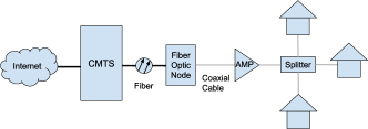
Figure 1: An overview of the Hybrid Fiber Coaxial (HFC) architecture.

A cable network has a hybrid fiber and coaxial (HFC) architecture. Figure 1 presents a schematic illustration of this architecture. The Cable Modem Termination System (CMTS) is located at the headend of an ISP, providing Internet connections to cable modems located at subscribers’ premises. A CMTS connects to devices called Fiber Optic Nodes (fNodes) via optical fibers. fNodes convert radio frequency (RF) signals to light signals and vice versa. They connect to individual homes or businesses via coaxial cables. An fNode typically serves a few hundred customers. For example, in our dataset, the average number of customers an fNode serves is around 250. To alleviate RF signal attenuation, RF amplifiers are deployed in the coaxial segments of an HFC network to ensure that RF signals delivered to end users are strong and of high quality.

Fault diagnosis remains a challenging issue in cable broadband networks. The coaxial segment of a cable network is prone to radio frequency impairments. In response to this challenge, the cable industry developed the PNM network monitoring framework to facilitate anomaly detection and fault diagnosis. A monitoring server sends periodic Simple Network Management Protocol (SNMP) [22] queries to collect performance metrics from customer cable devices as well as a CMTS. We refer to such data as PNM data.

II-B Datasets

For this study, an anonymous cable ISP (ISP-X), provided us with the PNM data collected from their networks and their customer tickets. We describe each dataset in turn.

PNM data

These data are collected from 70k+ customer devices and span a period of 14 months. A monitoring server collects the data approximately every 4 hours in-band. According to ISP-X, their infrastructure cannot support a shorter collection interval. PNM infrastructure [7] can collect both upstream (from a customer device to the CMTS) and downstream (the reverse direction) telemetry data in DOCSIS 3.0 and 3.1 cable devices. At the time of this study, ISP-X did not automatically collect downstream PNM data (partly because their daily operations did not depend much on PNM data prior to this study and collecting downstream PNM data is more resource-consuming as there are more downstream channels than upstream channels). Therefore, this study is based on upstream PNM data.

Each data collection point includes the several fields relevant to this study:

• Timestamp: the time at which the data point was received by the collection server.

• Anonymized device id: the hashed MAC address of a customer device.

• fNode: the identifier of the fiber optic node serving this device.

• SNR: the signal-to-noise ratio of a customer device’s transmission signal measured at a CMTS.

• Tx Power: the signal transmission power when a cable device sends a signal. This signal is recorded by a customer’s device and collected by the collection server from each cable device.

• Rx Power: the power of the received signal at the CMTS.

• Pre-Equalization Coefficients: the coefficients used by the pre-equalizer component in a customer device to compensate for linear signal distortions in coaxial cables.

Customer tickets

ISP-X creates a customer ticket to document how it handles a customer call. Each ticket contains several fields, including the customer’s account number, the ticket open time, the ticket close time (if any), a short description of the problem and its actions, and a category of the issue based on the ISP’s diagnosis. The category includes two classes: a part-of-primary ticket or not. The last field is crucial to this work. A part-of-primary ticket indicates that the ISP considers the issues the customers are experiencing a maintenance issue. Thus, it groups the tickets as one conceptual “primary” ticket. All part-of-primary tickets that belong to the same maintenance issue have the same primary ticket identifier. In this work, we refer to part-of-primary tickets as maintenance tickets and other infrastructure-related tickets as service tickets.

The customer ticket data we obtain span over the same period as the PNM data and are from customers located within the same networks.

II-C Ethical Considerations

The PNM data we received includes encrypted cable devices’ MAC addresses and scrambled location data (latitude + $noise_{1}$ and longitude + $noise_{2}$). Other PNM data are related to the physical signal properties of the cable devices. We discussed the data and the scope of this research with the IRB of our organization before conducting this work. The IRB determined that this work does not meet the definition of research with human subjects and it is appropriate for us to conduct this study. This work raises no other ethical concerns.

II-D Related Work

PNM Best Practice

The PNM best practice document [3] proposes to use a clustering algorithm to separate maintenance issues from service issues using the pre-equalization coefficients collected from cable devices. Pre-equalization coefficients are frequency-domain data and capture signal distortions in the frequency domain. Each cluster produced by the algorithm corresponds to a group of cable devices sharing a similar signal distortion at one PNM data point. However, these distortions may have already been compensated for and do not manifest themselves as user-perceivable performance issues. In addition, pre-equalization coefficients at each data point only reflect the instantaneous signal distortions and are prone to noise fluctuations. We find them ineffective in detecting network performance issues (§ V-B). Therefore, this work does not use them as features for either anomaly detection or fault classification.

Similarly, Volpe et al. [25] propose to use the full band spectrum (both upstream and downstream) data and apply DBSCAN [4] to group cable devices sharing the same anomalous spectrum patterns to reduce operational wastage caused by erroneous dispatches. The authors acknowledge in their work that there are no good approaches to tune the hyper-parameters of the system to set an anomaly detection threshold and the work does not include the experimental evaluation of the effectiveness of the proposed approach.

Different from previous approaches, TelApart treats PNM data as time-series data and applies clustering techniques using the time-domain similarity of PNM data. It tackles the challenges associated with time-domain data, such as data incompleteness and alignment problems commonly encountered when data are collected unreliably in production systems.

CableMon

CableMon [9] treats PNM data as time-series data. Differently, it focuses on the task of determining an anomaly detection threshold for a PNM metric associated with a cable device. CableMon defines ticketing rate, i.e., the average number of customer tickets created in a unit of time, as the statistics guiding its anomaly detection. Intuitively, the ticketing rate measures how frequently customer tickets are reported for a certain device. The authors of CableMon observed that the higher the ticketing rate is, the more likely there is a fault.

TelApart is inspired by this per-device anomaly detection work, with the observation of a gap in distinguishing network fault types. Although CableMon can tell if a single device has ongoing anomalies, it still cannot help ISPs determine the best team (maintenance or service) to dispatch. TelApart can not only assist with the decision of whether there is an anomaly, but also assist with the type of dispatch.

Other Related Work

Orthogonal to TelApart, previous study [8] has modeled characteristics of cable network faults and showcased physical-layer transmission errors are significant. There exists other fault detection work in the domain of cable broadband networks  [13, 20, 3, 12, 28, 5]. However, this body of work either uses static anomaly threshold settings or requires manual labeling of PNM data. There also exist tools that aim to assist ISPs’ manual troubleshooting by offering visualization and suggestions to operators [16, 21, 25, 26]. TelApart aims to automate fault diagnosis without manually labeled data and is orthogonal to this work. It can be enhanced with the visualization tools. Likewise, it is possible to design a fault diagnosis system for cable networks with manually labeled PNM data and more advanced machine learning techniques [6]. We chose to explore the design without labeled PNM data and evaluate the hypothesis of whether such a design can be effective.

III Design Rationale

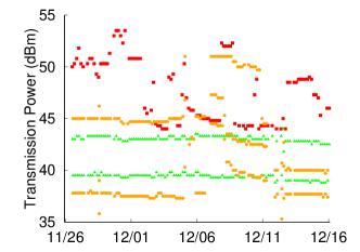
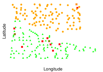
Figure 2: Figure (a) shows how the transmission powers of several cable devices in the same fiber optical node fluctuate over time. Orange dots are devices that show the same anomalous transmission power patterns. Green triangles are devices that show normal patterns. Red squares are devices that show distinct anomalous patterns. Figure (b) shows the locations of the cable devices using the same colored icons.

We aim to develop an easy-to-deploy fault diagnosis system that can automatically distinguish maintenance issues from service issues in cable broadband networks. At first glance, this appears to be a straightforward task: all we need is a machine learning classifier that automatically classifies PNM data collected from each cable device as healthy, with a maintenance issue, or with a service issue. Nevertheless, this simple problem is complicated by several practical challenges that need to be addressed.

III-A Challenges

The initial challenge we face is the high cost and time involved in acquiring high-quality labeled PNM data. Those data are proprietary and it requires specialized expertise to identify anomalies accurately. A domain expert must examine a large number of cable devices over a sufficiently long period of time to cover all possible anomalous patterns. As an example to illustrate how tedious this task is, we depict the transmission powers of six cable devices in Figure 2. A domain expert must label thousands of such figures at a minimum to generate useful training data.

One might be attempted to utilize customer tickets as automatic labels: when there is a maintenance ticket, we label the data point as maintenance, and vice versa. In the absence of a ticket, we label a data point as healthy. However, our attempt to adopt this approach revealed its ineffectiveness. This is because customer tickets are highly prone to noise: customers may call when there are no infrastructure problems and may not call when there are problems. Moreover, according to ISP-X, their diagnosis of a maintenance or service issue is inaccurate. Therefore, this ticket-based-labeling approach does not lead to high-quality labels.

The second challenge we face is that a machine learning model unavoidably incorporates many hyper-parameters. However, cable ISPs operate in vastly different conditions. For instance, each may use different frequency channels or operate in varying climatic conditions. Therefore, each ISP must label its own PNM data to train and tune the model for effective fault diagnosis and to mitigate model drift. Yet many cable ISPs do not have dedicated personnel for such tasks.

Third, unsupervised learning models compare the similarity of their input data to find similar patterns. However, PNM data are collected unreliably and contain many missing and duplicated data points. Furthermore, the data collection system introduces randomness to avoid network congestion. Thus, the data collected from each device are not temporally aligned. It is preferable to compare data points that are collected close in time to produce meaningful comparisons. However, using the raw PNM data as inputs may misalign data points that are distant in data collection times, thereby rendering similarity comparisons inaccurate.

III-B Goals

To mitigate the practical challenges mentioned above, we ask the following question: is it feasible to develop a fault diagnosis system for cable networks using unlabeled PNM data and hyperparameters that are automatically tuned? To answer this question, we identify the following design requirements for TelApart:

No manual data labeling:

TelApart must not rely on labeled data for model training or tuning.

Automated hyper-parameter tuning:

TelApart must be able to tune its hyper-parameters programmatically without human intervention.

Effective despite unreliably-collected data:

TelApart must effectively separate maintenance issues from service issues using the existing PNM data that include missing, duplicated, and unaligned data across cable devices.

III-C Motivation

To gain insight into how to separate a service issue from a maintenance issue, we manually examined several anomaly patterns by plotting PNM metrics described in § II-B. Figure 2 shows an example. In this figure, we sampled the transmission power levels of devices with three anomaly patterns from an fNode. The orange dots show the transmission power levels of three devices that exhibit similar anomalous patterns in the changes of their transmission powers. When a noise leaks inside a cable transmission channel, a device increases its data transmission power to overwhelm the noise. So a sudden increase in transmission power is an indicator of noise invasion. The green triangles show the transmission power levels of two devices that are not impacted by the noise. The red squares show the transmission power levels of a device that exhibits a different anomalous pattern.

Figure 2 shows the geographic distribution of the devices in the fNode. We use the same color coding schemes to plot the devices. The orange dots plot the scrambled geographic locations of the devices that exhibit similar anomalous patterns as depicted in Figure 2. Each red square shows the scrambled geographic location of a device that exhibits a distinct anomalous pattern. And the green triangles show the locations of the devices that do not exhibit any anomalous pattern.

From this data visualization step, we gained the conceptual understanding that we could use clustering to distinguish a maintenance issue from a distinct service issue. In addition, we observe that fault detection is independent of clustering, as both the healthy devices (the green group) and the unhealthy ones (the orange group) form distinct clusters. These observations, together, motivate TelApart’s architecture, which we describe next.

IV Design

In this section, we describe TelApart’s design, including the programmatically approach to set hyper-parameters.

IV-A System Overview

Figure 3: An overview of TelApart’s design. $C_{thr}$ is a threshold specified by a network operator based on its network topology.

We make several design choices to address the practical challenges TelApart’s design faces. First, we decouple common PNM data pattern recognition from fault detection, as the former can be accomplished with unsupervised learning (§ IV-B).

Second, we design optimization techniques that use customer tickets and operational knowledge as clues to tune hyperparameters of an unsupervised learning model and set the anomaly detection thresholds programmatically. While customer tickets are noisy and cannot be used for precisely labeling PNM data, they still offer valuable information: when there is a customer ticket, a network is more likely to experience an infrastructure problem than when there is no customer ticket. This observation motivates the design of using the ticketing rates of maintenance tickets to choose the values of TelApart’s hyper-parameters (§ IV-C).

Finally, we design techniques to pre-process PNM data. After pre-processing, each device will have the same number of data points so we can feed the pre-processed data to a clustering model (§ IV-F).

Figure 3 shows the workflow of TelApart. We first pre-process the selected raw PNM features from all cable devices in a fiber optical node. After pre-processing, all devices have the same number of data points and these data points are aligned in time. We then feed the pre-processed data to a clustering model, which outputs clusters of devices that share similar PNM data patterns. For each cluster, we detect whether it exhibits any anomalous pattern. A cluster is identified as “healthy” if there are no anomalous patterns. Otherwise, we distinguish a maintenance issue and a service issue with the cluster size: if an anomalous cluster has more than $C_{thr}$ devices, we classify it as experiencing a maintenance issue. Otherwise, the cluster is marked as a service issue. The threshold $C_{thr}$ is a configuration parameter, chosen as 5 by ISP-X according to their physical networks in this work, i.e., the majority of amplifiers serve more than 5 devices.

Each invocation of TelApart takes the PNM data from cable devices connected to one fNode, as those devices share the same RF domain.

TelApart’s clustering component takes pre-processed PNM data as input and outputs groups of cable devices that share similar PNM data patterns. We select a subset of independent PNM metrics as features and cluster cable devices by each feature. We describe feature selection in § IV-D. Each input feature vector includes the pre-processed PNM data points collected between a time interval $(t-d,t]$, where $t$ is the time of diagnosis and $d$ configures a look-back duration, e.g., one or two days. In practice, ISP-X collects PNM data every 4 hours, and all devices have 3 upstream channels. Because ISP-X intends to perform daily detection, we set $d=1$ day. In this case, we obtain 6 data points in each channel, a total of 18 when there is no data loss. We also varied $d$ from 1 to 7 days and did not observe any significant performance difference, indicating a longer look-back window does not benefit the daily detection.

TelApart’s pre-processing unit aligns each PNM feature vector in time so we can compare the similarity of any two devices’ feature vectors. We define a similarity comparison function for each PNM feature and describe them in § IV-D.

IV-B Clustering

We consider and evaluate several clustering algorithms [4, 27, 23, 24] and find that the average-linkage hierarchical clustering algorithm [27] performs the best (§ V-C). At a high level, this clustering algorithm works as follows. For each feature $f$ we selected, the clustering algorithm aims to group devices with similar feature vectors together until the similarity between groups of devices falls below a threshold $s_{f}$. Specifically, it first treats each device (described by a feature vector) as a single cluster. Second, it calculates the similarity between every pair of clusters and finds two clusters with the highest similarity value. The similarity between two clusters is calculated by averaging all similarity values between pairs of devices in the two clusters. Third, the algorithm merges the two clusters with the highest similarity value into a single cluster. Next, the algorithm repeats the second and third steps until only one cluster is left or the highest similarity value between any two clusters is less than the similarity threshold $s_{f}$. Finally, the algorithm outputs the clusters that have not been merged.

IV-C Setting the Similarity Threshold

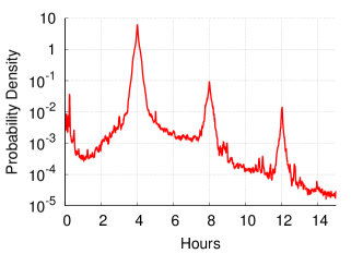
Figure 4: This figure shows the probability density function of data collection intervals.

The similarity threshold $s_{f}$ for each feature $f$ is an important hyper-parameter and TelApart’s performance is sensitive to its value. If we set the threshold too high, TelApart may separate devices that are affected by the same network fault into multiple clusters. Conversely, if we set the threshold too low, it may group devices that are affected by different maintenance issues into the same cluster.

How do we choose a proper similarity threshold? If we had labeled training data, we could use the grid-search method [14] to iterate over possible values and set the threshold that minimizes clustering errors. Lacking of labeled data, we instead use customer ticket statistics to guide the search for the similarity threshold. Our insight is that if TelApart correctly identifies groups of devices that are impacted by the same maintenance issue, then on average, we should observe a higher fraction of maintenance tickets reported by these groups of devices than other devices. In contrast, if TelApart partitions the cable devices rather randomly, then we should not observe significant statistical differences of the reported maintenance tickets among different groups.

Motivated by this insight, we naturally evolve the ticketing rate of CableMon (§ II-D) to maintenance ticketing rate and devise the following mechanism to set the similarity threshold $s_{f}$ for each PNM feature we use. We partition the PNM dataset we have into a training set and a testing set. For each data point $i$ in the training set and for each possible value of $s_{f}$, we use TelApart to diagnose whether a device $j$ is impaired by an infrastructure fault and the type of fault, as shown in Figure 3. If TelApart considers a device experiencing a maintenance issue, we mark this collection period of this device as a maintenance event. We use $I_{i,j}$ to denote the length of the data collection interval between data points $i$ and $i-1$ of device $j$. Similarly, if TelApart considers a device experiencing a service issue, we mark the collection period of the device as a service event. We then count the number of maintenance tickets reported by all devices during all collection periods that are marked as maintenance issues and compute a maintenance ticketing rate during maintenance events as

$$R_{m,M}=\frac{K_{m,M}}{\sum_{i,j}I^{M}_{i,j}}$$ (1)

where $K$ denotes the number of tickets, $R$ denotes the ticketing rate, the first subscript $m$ denotes maintenance tickets, and the second subscript $M$ denotes a diagnosed maintenance issue, and $I^{M}_{i,j}$ is the length of a collection period that is marked as experiencing a maintenance issue.

We also count the number of maintenance tickets $K_{m,S}$ reported by all devices during all collection periods that are marked as service issues. We compute a maintenance ticketing rate during service events as

$$R_{m,S}=\frac{K_{m,S}}{\sum_{i,j}I^{S}_{i,j}}$$ (2)

where $S$ indicates a diagnosed service issue, and $I^{S}_{i,j}$ is the length of a collection period marked as experiencing a service issue. We define the maintenance Ticketing Rate Ratio ($TRR_{m}$) as

$$TRR_{m}=\frac{R_{m,M}}{R_{m,S}}$$ (3)

For each feature $f$ TelApart uses, we use grid-search to find the similarity threshold value $s_{f}$ that maximizes $TRR_{m}$. In Appendix D, we prove that the $s_{f}$ maximizing $TRR_{m}$ yields the optimal clustering result: it minimizes both false positives (i.e., a device without any maintenance issues is detected as with a maintenance issue) and false negatives (i.e., a device with a maintenance issue is detected as without any maintenance issues). Intuitively, based on ISP-X’s fault diagnosis process, maintenance tickets contain fewer false positives than service tickets. Thus, if we assume the operator-labeled maintenance tickets approximate the unknown but existing ground truth of maintenance events and TelApart’s fault detection mechanism is accurate, then the maintenance ticketing rate during maintenance events approximates TelApart’s true positives and the maintenance ticketing rate during service events approximates TelApart’s false negatives. Maximizing the ratio of the two ticketing rates leads to high true positives and low false negatives.

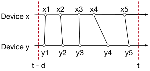
Figure 5: This figure shows an example that without inferring missed data points, a naive alignment algorithm may pair up two data points $x_{4}$ and $y_{4}$, which are not close in time.

IV-D Feature Selection and Comparison

The PNM system collects many metrics, but for simplicity and computation efficiency, it is desirable to use only a minimum set of effective and independent features for fault diagnosis. We describe how we choose the features TelApart uses and the similarity function we choose to compare each feature.

We start with a candidate set of features that CableMon [9] finds effective in detecting infrastructure faults in cable broadband networks. Some of these features contain the instantaneous values measured at the data collection times, while others are cumulative values (e.g. codeword error counters) over time. We find that the instantaneous metrics, including SNR, Tx power, and Rx power, are effective features for grouping devices with shared maintenance issues together - they achieve high maintenance ticketing rate ratios when used as clustering features. On the other hand, cumulative metrics, although effective in detecting anomalies [9], are not effective as clustering features. For example, the values of codeword error counters are affected by whether users actively use the Internet or not. Devices that share the same maintenance issue may or may not have highly correlated codeword error counters if the subscribers’ usage patterns differ. Hence, this work uses only instantaneous metrics: SNR, Tx power, and Rx power. Among them, Tx and Rx powers are statistically correlated. Finally, we retain two independent features: SNR and Tx power for clustering.

We use the Pearson correlation coefficient [2] as the similarity metric to compare two devices’ SNR and Tx power values. We choose the Pearson correlation coefficient because it measures the linear correlation between two vectors. When a maintenance issue occurs, the impacted devices’ PNM metrics will increase or decrease simultaneously to adapt to the changed network conditions. Pearson coefficient can capture the synchronized changes well regardless of the absolute values of two devices’ PNM metrics, as the baseline values of different devices’ Tx powers could differ significantly.

A new feature we uncover in this work is a feature vector that encodes the missed data collection points. TelApart’s data pre-processing module can infer which data points each device misses. Many factors can cause data missing, e.g., the loss of a PNM data collection request or response, a faulty device, or a network outage. Intuitively, if a group of devices simultaneously miss data collection points, it could indicate a maintenance issue. Led by this insight, we generate a binary feature vector with 0 indicating a missing data collection point. We find that using this feature vector (referred to as missing hereafter) as a clustering feature leads to a high maintenance ticketing rate ratio. So we also include missing as a clustering feature. We use one minus the normalized hamming distance as the similarity metric between two devices’ missing features. Normalized hamming distance is a metric that computes the distance between two binary strings [17] and is suitable for comparing the similarity of two binary feature vectors.

IV-E Fault Detection

After TelApart’s clustering module identifies groups of devices sharing similar PNM data patterns, it invokes a fault detection module on each cluster (which could contain a single device), as shown in Figure 3. When the module detects an anomaly for any device in a cluster, it flags the entire cluster as anomalous.

Fault detection is relatively independent of TelApart’s data pre-processing and clustering modules. TelApart adopts the state-of-the-art fault detection techniques proposed in CableMon [9], as they can detect infrastructure faults using PNM data without labeled training data nor static thresholds. CableMon [9] detects network faults with dynamic thresholds on performance metrics of a device’s PNM data. A device is detected with an anomaly if there are performance metrics below or beyond the corresponding threshold. CableMon elaborately selects these thresholds maximizing the ticketing rate (§ II-D) such that the detected anomalies are associated with the most customer tickets, which implies larger impacts on user experience and more operational costs. TelApart treats these fault detection thresholds as hyper-parameters auto-tuned by CableMon. However, the techniques themselves cannot differentiate the types of faults. TelApart can incorporate any fault detection module that meets its design goals listed in § III.

IV-F Data Pre-Processing

To compare the similarity of two devices’ PNM data, it is desirable to compare data points collected closest in time together. However, the PNM infrastructure uses SNMP to collect data, which is unreliable. We observe many missed and duplicated data points in our dataset. In addition, in the same data collection epoch, different devices respond at different times to avoid congestion. So the timestamps of different devices’ data points could span a wide range even in the same data collection epoch.

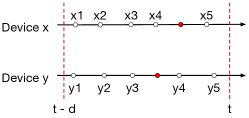
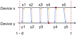
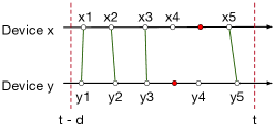
Figure 6: This figure shows the steps in TelApart’s data pre-processing algorithm.

Concretely, we depict the distribution of the time intervals between a device’s two adjacent data points for all devices in our dataset in Figure 4. As we can see, the modes of the distribution are multiples of four hours, which is the default data collection interval of ISP-X. If the interval between two adjacent data points is close to eight, then it is highly likely that there is a missed data point, and so on. The bump near 0 indicates duplicated data points.

However, there are many data collection intervals that have lengths between two adjacent multiples of fours, as shown in Figure 4. For example, if two data points are six hours apart, it could either be the case of a missed data point or the case of a delayed data collection point. If we cannot differentiate these two cases, we may produce a suboptimal alignment that does not compare data points collected closest in time together.

Figure 5 shows an example. Suppose TelApart runs at time $t$ and its look-back window $(t-d,t]$ includes five data points from cable devices $x$ and $y$, respectively. If we greedily match each data point in one device to its closest data point in the other device, we will produce an alignment as shown in Figure 5, where data point $x_{4}$ is aligned with data point $y_{4}$. However, a better alignment, shown in Figure 6, is that $x_{4}$ and $y_{4}$ are not paired together so the collection time difference in each paired data point is less.

We design a data pre-processing algorithm to align two devices’ PNM data points such that it minimizes the time difference between any two aligned data points. This algorithm involves two steps. In the first step, we infer which data collection points are missing as shown in Figure 6. The red dots are the missed data points the algorithm infers. We note that ISP-X’s PNM data do not include a sequence number for each PNM record nor the timestamp when a PNM collection request is sent. If other cable ISPs have such information, they can skip this step, as such information makes a device’s missed data points explicit. In the second step, we apply a bijection function to align the data points collected from two devices so that each data point in one device is paired with the closest data collection point in the other device as shown in Figure 6. We keep the pairs with bi-directional alignments as the final result, as shown in Figure 6.

To infer missed data points, we use an offline algorithm to determine a threshold $L_{missing}$ as another hyper-parameter of TelApart. When the data collection interval between a device’s two adjacent data points exceeds the threshold, it is highly likely that there is a missed data point. We use this threshold to determine a missing data point at the time of diagnosis. We note that this threshold is a hyper-parameter, but we choose its values programmatically using the operational knowledge: the default data collection interval.

As we observe in Figure 4, if we project the data collection times of all devices in the same fiber optical node on the timeline over a long duration, we will observe distinct clusters corresponding to each data collection epoch, where the distances between the centers of two adjacent clusters are multiples of the default data collection interval. If the distance between the centers of two clusters exceeds the default data collection interval, it indicates that there is a missed data point for the entire fNode. Within each cluster, if a particular device does not have a data point in the cluster, it indicates that the device misses a data point. With this knowledge, we can determine an optimal threshold $L_{missing}$, such that if we use the threshold to infer a device’s missed data points, the results match the earlier cluster-based inference results the best. We show the details of our algorithm that determine the optimal of $L_{missing}$ in Appendix B.

We include the pseudo-code and more details of TelApart’s data pre-processing algorithm in Appendix A, B, and C. We prove in Appendix C that TelApart’s data pre-processing algorithm produces pair-wise aligned data points between two devices that minimize the time difference for each pair of aligned data.

We note that the PNM infrastructure collects PNM data for each upstream channel. TelApart pre-processes each channel’s PNM data and then for each feature, it concatenates the data points from each channel into one single feature vector. For instance, the data we have include three upstream channels. Each feature vector is the concatenation of pre-processed PNM data from all three channels.

V Evaluation

TelApart’s main goal is to separate maintenance issues from service issues. In this section, we evaluate how well TelApart achieves this goal.

V-A Establishing Evaluation Metric

Central to TelApart’s design is a machine learning model that classifies a device’s state as healthy, experiencing a maintenance issue, or experiencing a service issue. It is challenging to evaluate its effectiveness as we do not have the ground truth. To address this challenge and to scale our evaluation, we develop metrics based on customer tickets.

Our assumption here is that if we detect maintenance issues, from a statistical view, customers who suffer from those issues will report more maintenance tickets compared to service tickets, and vice versa. Therefore, we define a normalized ticketing rate as a metric to evaluate TelApart’s fault diagnosis accuracy. Recall that in Eq 1 and Eq 2, we define two ticketing-rate variables $R_{m,M}$ and $R_{m,S}$ as the number of maintenance tickets averaged over the total length of data collection periods TelApart diagnoses as experiencing a maintenance and a service issue, respectively. We can define ticketing rate variables $R_{s,M}$ and $R_{s,S}$ correspondingly where $s$ stands for service tickets.

Because an ISP’s fault diagnosis is inaccurate, we assume for each type of ticket, there exists random errors. To discount those errors, we define a baseline ticketing rate $R_{t}$ as the number of tickets of type $t$ ($t$ is either maintenance or service tickets) averaged over all devices in a fiber optical node and the entire data collection period.

A normalized ticketing rate $\overline{R_{t,E}}$ of a ticket type $t$ and a diagnosis type $E$, where $E$ is either a maintenance issue or a service issue is defined as $\frac{R_{t,E}}{R_{t}}$. Assuming that an ISP receives much higher frequency of customer calls during a true maintenance or service issue, if a fault diagnosis system can accurately diagnose a maintenance or service issue, we will observe high normalized ticketing rates for both maintenance and service issues. In contrast, if a system cannot effectively identify maintenance or service issues, we would observe a normalized ticketing rate close to 1.

To summarize, we define four normalized ticketing rates: $\overline{R_{m,M}}$, $\overline{R_{s,M}}$, $\overline{R_{m,S}}$, and $\overline{R_{s,S}}$. For an algorithm that can detect service or maintenance issues from PNM data, we should observe the following 4 invariants:

$$\overline{R_{m,M}}>\overline{R_{s,M}}>1,\quad\overline{R_{m,M}}>\overline{R_{m,S}}>1,$$

$$\overline{R_{s,S}}>\overline{R_{m,S}}>1,\quad\overline{R_{s,S}}>\overline{R_{s,M}}>1$$

and high value of $\overline{R_{m,M}}$ and $\overline{R_{s,S}}$ indicates better performance.

V-B Comparing with PNM Best Practice

The official PNM document from CableLabs [3] introduces an algorithm that uses each PNM data point’s pre-equalization coefficients as a feature vector for clustering devices impacted by the same linear RF distortion, which can be caused by either a service issue or a maintenance issue. Therefore, as a comparison, we implement this algorithm and set its clustering similarity threshold in the same way as we tune those thresholds for TelApart’s features, and compare the normalized ticketing rate defined in § V-A.

To set up the comparison experiment, We split the 14-month PNM data we have into two sets: an 11-month training set (from Jan 2019 to Nov 2019) and a 3-month test set (from Dec 2019 to Feb 2020). We use the training set to determine the values of TelApart ’s hyper-parameters and the test set to evaluate TelApart ’s performance.

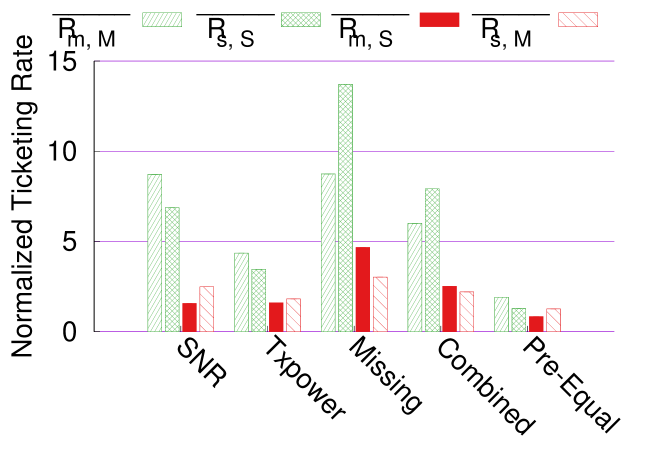
Figure 7: The normalized ticketing rates for various combinations of ticket type and diagnosis result, where $m$ denotes maintenance tickets, $s$: service tickets, $M$: TelApart-diagnosed maintenance issues, and $S$: TelApart-diagnosed service issues.

Figure 7 shows the results when we run TelApart on the test dataset. We show the ticketing rates for faults detected by each independent feature as well as the “Combined” result detected using all TelApart’s features. For each individual metric, SNR, Tx Power and Missing, both the normalized ticketing rates $\overline{R_{m,M}}$ and $\overline{R_{s,S}}$, which suggests accurate diagnoses, are much higher than $\overline{R_{m,S}}$ and $\overline{R_{s,M}}$ for all TelApart’s features. For the missing feature, the normalized service ticketing rate during a TelApart-diagnosed service issue is as high as $13$, suggesting that missing data points are highly predictive of service issues. We also calculate the combined normalized ticketing rates as the combination of the three metrics TelApart used, and it shows a good performance as well.

In contrast, for pre-equalization coefficients, we find that all combinations of normalized ticketing rates are slightly above 1, suggesting that they are not effective in detecting or diagnosing customer-reported faults. Our explanation is that those coefficients are designed to compensate for signal distortions in cable networks. They detect distortions that are already compensated for, but are not effective in signaling un-compensatable anomalies that lead to customer tickets.

We also compute the normalized ticketing rates for both maintenance and service issues when a device is healthy. All values of those normalized ticketing rates are between $[0.891,1)$, suggesting that TelApart correctly identifies healthy networking conditions. The normalized ticketing rates in healthy periods are less than 1 because the healthy periods have fewer than average tickets. We do not show them in Figure 7 for clarity.

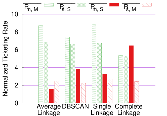
Figure 8: The normalized ticketing rates of SNR for various cluster algorithms of ticket type and diagnosis result.

V-C Comparing with Different Choices

In the design of TelApart, we design a unique preprocessing method that includes missing position inference and time series data alignment. Meanwhile, TelApart adopts the average linkage hierarchical clustering algorithm to cluster the cable devices that share the same abnormal patterns. In this subsection, we compare our design choice with other popular algorithms, to show our design choice outperforms other algorithms. For the clustering algorithm, we compare our choice with three alternatives: DBSCAN, single-linkage, and complete-linkage clustering algorithms. For the preprocessing, we contrast our choice with resampling, a popular preprocessing method for irregularly sampled time series data.

For each comparison, we replace our choice with alternatives and run TelApart to compare the normalized ticketing rate defined in § V-A. Besides, in order to validate the performance of a clustering algorithm, we manually labeled a small set of PNM data in a format similar to Figure 2 as the ground truth of this evaluation. We use customer tickets to locate the time periods where faults are likely to occur. If a group of devices (with group size exceeding $C_{thr}$) shows a common anomalous pattern, we label this group of devices as experiencing a maintenance issue. If there are only one or a few devices are affected, we label it as a service issue. We label all devices that show no anomalous patterns as healthy. We learned from ISP-X that this process resembles how they manually diagnose a network anomaly.

We started the inspection by choosing 50 maintenance tickets and used the tickets’ start and close time to guide the search for anomalous patterns. We were able to obtain 16 groups of maintenance issues that impact nearly 700 devices. Since we must inspect all devices sharing the same fiber optical node for each maintenance ticket, we were also able to identify 113 devices that were affected by service issues. We carefully verified the labeling results with ISP-X’s experts to guarantee the labeling accuracy.

This manual labeling process is cumbersome and error-prone. It took two-person-week to obtain these labels. We intentionally did not expand into more labels to ensure the labeling accuracy. We note that this manually labeled set covers only a small fraction of anomalous patterns and is not suitable for training a high-quality classifier.

We run the clustering algorithm on PNM data we label and compare their cluster results with our labeled results. We choose two widely used metrics for evaluating each clustering algorithm: the Rand Index (RI) [19] and the Adjusted Rand Index (ARI) [10].

We compute RI by comparing the partitions produced by a clustering algorithm with the ground truth partition. If two devices are in the same cluster in both partitions, we count it as a true positive ($TP$). Conversely, if two devices are in the same subset in the partition produced by a clustering algorithm, but they are in different subsets in the ground truth partition, we count it as a false positive ($FP$). True negatives ($TN$) and false negatives ($FN$) are defined accordingly. RI computes the fraction of true positives and negatives divided by the total pairs of devices: $\frac{TP+TN}{TP+TN+FP+FN}$. Its maximum value is 1. The higher the RI, the better the clustering result. ARI adjusts for the random chances that a clustering algorithm groups two devices in the same cluster by deducting the expected RI ($\mathbb{E}(RI)$) of a random partition: $\frac{RI-\mathbb{E}(RI)}{1-\mathbb{E}(RI)}$.

Clustering Algorithm

Within the architecture of TelApart, the average linkage hierarchical clustering algorithm is employed to categorize devices affected by the same network anomaly. A salient challenge is the indeterminacy of the distinct pattern count. Given this inherent uncertainty, clustering algorithms that mandate the specification of the number of clusters, represented by the hyper-parameter $k$, are inherently inconsistent with our design objectives. In the context of TelApart, it is imperative to employ algorithms capable of discerning the optimal number of clusters autonomously, circumventing the limitations presented by the need for predefined cluster counts. Therefore, we compare TelApart’s clustering algorithm choice with three popular clustering algorithms that are not contingent on the predefined $k$ value, including DBSCAN, single-linkage, and complete-linkage clustering algorithms.

	Average Linkage	DBSCAN	Single Linkage	Complete Linkage
RI	0.91	0.84	0.83	0.83
ARI	0.83	0.65	0.64	0.66

TABLE I: Rand Index and Adjusted Rand Index for various clustering algorithms.

Table I shows the comparison results. TelApart achieves an RI of 0.91 and an ARI of 0.83, respectively. TelApart’s choice outperforms other clustering algorithms.

Figure 8 shows the normalized ticketing rate for SNR (the result of Tx Power is similar but skipped due to space limitation). The figure shows that the average linkage hierarchical clustering algorithm achieves the highest $\overline{R_{m,M}}$ and $\overline{R_{s,S}}$, which suggests the best performance. It is pertinent to note that the comparative analysis does not encompass the normalized ticketing rate for missing data. This exclusion is attributed to the observation that various clustering algorithms exhibit analogous performance metrics in this dimension. The uniformity in the normalized ticketing rate for missing data across different algorithms is caused by the characteristic that the missing vectors are not subjected to irregular sampling, and the missing vector is a 0-1 vector, rendering the comparative distinctions negligible.

Preprocessing

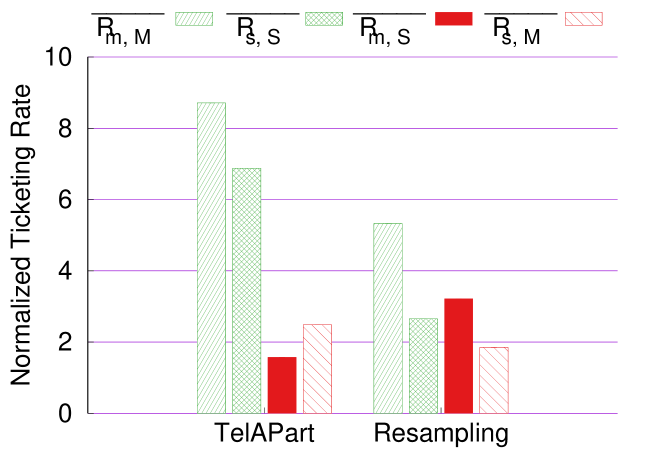
Figure 9: The normalized ticketing rates of SNR for two preprocessing algorithms of ticket type and diagnosis result.

A common method to handle irregularly sampled time series data involves its transformation into uniformly spaced intervals through resampling [15]. Each time series is systematically restructured onto a consistent grid, necessitating the application of interpolation techniques or, in instances of noise prevalence, regression models to approximate the inherent continuous temporal dynamics.

We employ a classic resampling technique to process the PNM data, utilizing linear interpolation to transform the data into a uniformly spaced 4-hour interval. This method effectively aligns the data points and mitigates the presence of missing data, resulting in a coherent and complete dataset. We then run the clustering algorithm TelApart adopts to demonstrate the effectiveness of our preprocessing algorithm.

	TelApart’s Preprocessing	Resampling
RI	0.91	0.74
ARI	0.83	0.35

TABLE II: Rand Index and Adjusted Rand Index for two preprocessing methods

Table II shows the comparison results. TelApart achieves an RI of 0.91 and an ARI of 0.83, respectively. TelApart’s preprocessing algorithm choice outperforms the classic resampling algorithm.

Figure 9 shows the normalized ticketing rate for SNR (the result of Tx Power is similar but skipped due to space limitation). The figure reveals that the preprocessing algorithm employed within TelApart outperforms alternative methods, as evidenced by the elevated values of $\overline{R_{m,M}}$ and $\overline{R_{s,S}}$.

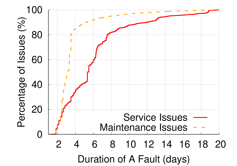
Figure 10: The cumulative distribution of how long a maintenance (or service) issue lasts.

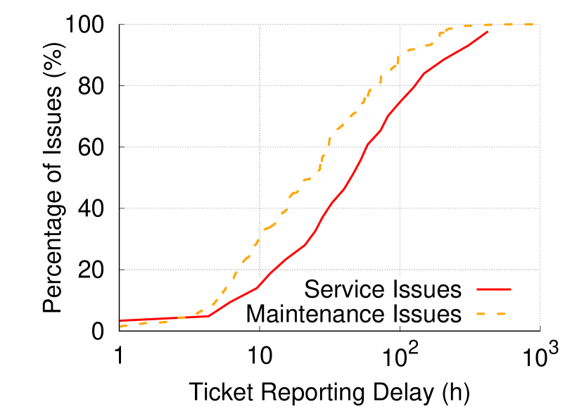
Figure 11: The cumulative distributions of ticket reporting delays for TelApart-diagnosed maintenance and service issues.

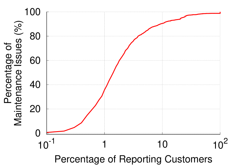
Figure 12: The cumulative distributions of reporting customers when a maintenance issue occurs.

V-D Fault Characteristics

An additional source of truth we have is how ISP-X processes customer calls and the definitions of maintenance and service issues. Due to the lack of any other source of truth, we use this operational knowledge to validate TelApart’s diagnosis accuracy.

Fault Duration

By ISP-X’s definition of the maintenance cluster size threshold, a maintenance issue impacts more customers than a service issue. Therefore, more customers are likely to call an ISP when a maintenance issue occurs than when a service issue occurs. If TelApart correctly differentiates a maintenance issue from a service issue, we would observe that the delay between when a maintenance issue occurs and when the first customer calls to be shorter than that when a service issue occurs. As a result, a maintenance issue is likely to be fixed sooner than a service issue.

To test this hypothesis, we compute the duration of a TelApart-diagnosed fault as follows. We run TelApart in batch mode on the test dataset and record the first time a fault is detected until the time the fault is no longer detected. In Figure 12, we depict the cumulative distribution of the fault duration for maintenance and service issues, respectively. As can be seen, 80% of the maintenance issues are fixed in 84 hours (3.5 days), while 80% of the service issues are fixed in 182 hours (7.6 days). This result further indicates TelApart’s diagnosis is accurate.

Ticket Reporting Delay

Figure 12 shows the distributions of ticket reporting delays for maintenance issues and service issues diagnosed by TelApart, respectively. We do not differentiate the first arrival ticket’s type for a TelApart-diagnosed issue, as it may be mis-labeled by an operator. We observe that when the ticket reporting delay exceeds a few hours, there is a significant difference between the ticket reporting delay distribution for maintenance issues and that for service issues. For example, for more than 50% of the maintenance issues diagnosed by TelApart, the first ticket arrives within 24 hours. In contrast, only for less than 31% of the service issues diagnosed by TelApart, the first ticket arrives within 24 hours. This difference again suggests that TelApart is able to separate maintenance issues from service issues effectively. Interestingly, when the ticket reporting delay is short, the ticket reporting delay distributions for maintenance and service issues overlap. We hypothesize that these tickets are impacted by severe issues so that any subscriber impacted by one of these issues reports immediately.

V-E User Ticketing Behavior

We are interested in studying what percentage of customers will make a trouble call when a customer-impacting maintenance issue occurs. This study does not serve the purpose of evaluation, but offers useful information to researchers and network operators. For this purpose, we examine each maintenance issue diagnosed by TelApart during the span of the entire dataset and measure the size of the anomalous cluster TelApart detects. We then count the number of customer tickets coinciding with the duration of the maintenance issue and divide it by the size of the cluster.

Figure 12 shows the cumulative distribution of the percentage of reporting customers for a maintenance issue. For more than 90% of the maintenance issues, 90% of the impacted customers will not make a call. The low percentage of reporting customers suggests that it is important for ISPs to periodically monitor their networks and proactively repair network impairments to improve the quality of experience for their customers. ISPs can invoke TelApart in the batch mode periodically to achieve this goal.

VI Conclusion

Cable ISPs can benefit from accurate and automated fault diagnosis for reducing operational costs caused by erroneous fault diagnoses. This work addresses a fault diagnosis problem present in cable broadband networks, i.e., how to distinguish a maintenance issue from a service issue. We develop TelApart, a system that uses the telemetry data readily available in cable broadband networks to automatically diagnose the type of fault. In TelApart’s design, we combine unsupervised learning, anomaly detection, and optimization techniques to eliminate the need for manually labeled training data and hand-tuning hyper-parameters. We also develop data pre-processing techniques to enable machine learning models on PNM data, which are unreliably collected and contain missing, duplicated, and unaligned data points. We use a small set of manually labeled data and customer ticket statistics to evaluate TelApart. The evaluation results show that when compared to the labeled data, TelApart achieves a Rand Index of 0.91. During TelApart-diagnosed maintenance (or service) events, a much higher than average frequency of maintenance (or service) tickets occur, further suggesting that TelApart can effectively distinguish maintenance issues from service issues. The cable ISP we collaborated with has confirmed the effectiveness of TelApart with field tests.

Appendix A Algorithm for Inferring Missing Data Points

Algorithm 1 Inferring Missing Data Points

1:$T_{a\_raw}=\{t_{1},t_{2},...,t_{n}\}$ $\triangleright$ The timestamp array of the time series data for device $a$

2:$T_{a}\leftarrow\{t_{1}\}$ $\triangleright$ The array to store both the valid timestamp and missing timestamp

3:for $i\$ from $2\$ to $n\$ do

4:     while $t_{i}$ - $t_{i-1}$ in $T_{a}$ ¿= $L_{missing}$ do

5:         insert a placeholder at $t_{i-1}+4hrs$ in $T_{a}$      

6:     insert $t_{i}$ in $T_{a}$

7:return $T_{a}$

This algorithm will iterate each data point once. Suppose the input data length is K, and the total number of devices is M. Then the time complexity of this algorithm for each device is O(K), and running this algorithm among all the devices will cost $O(M\times K)$.

Appendix B Determine the Optimal Missing Threshold

The algorithm for inferring missing data points required an accurate missing threshold $L_{missing}$. It is challenging to find the best $L_{missing}$ because if we set this value too aggressively, we may infer more missing data points than ground truth. And if we set this value too conservatively, we may fail to infer some missing data points.

To overcome this challenge, we developed an algorithm to determine the optimal missing threshold. The high-level idea is, using a given $L_{missing}$, we can infer the missing data points in our PNM data. We then compare our inferred results with the ground truth we generated, and select the $L_{missing}$ that gives us the highest accuracy. In TelApart, all the steps are automatic to cable ISPs once they input the PNM data and the length of the default data collection interval $L$. We will first introduce the method we use to generate the ground truth of missing data points, then describe how we use this ground truth to guide us to find the best $L_{missing}$.

Generate the Ground Truth of Missing Data Points

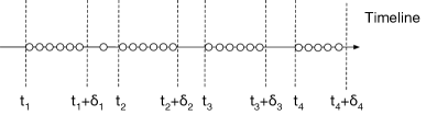
Figure 13: This figure shows the data collection time for all devices in the same fNode.

Figure 13 shows an example of the data collection time for all devices in the same fNode in our data. ISP-X starts to collect the PNM data from this fNode at time $t_{1}$, $t_{2}$, $t_{3}$, and $t_{4}$, and finishes each round of data collection at time $t_{1}+\delta_{1}$, $t_{2}+\delta_{2}$, $t_{3}+\delta_{3}$, and $t_{4}+\delta_{4}$, respectively. The time interval between $t_{1}$, $t_{2}$, $t_{3}$, and $t_{4}$ are roughly the same as the default data collection interval $L$ (4 hours in this example). At each data collection period, PNM data will be collected from all devices in random order. Therefore, it is possible that the PNM data from a device was collected at $t_{1}$ in the first period, and was collected at $t_{2}+\delta_{2}$ in the second period. This observation provides evidence of why inferring missing data points and determining the optimal missing threshold is a challenge.

Figure 13 shows the data points have a high density in each data collection period, while between two periods, the data point distribution is very sparse. This inspires us to adopt the density-based clustering algorithm to find each data collection interval. Once we observed the PNM data from a device are only collected at the first and the third data collection periods, then we can infer that in the second data collection period, the PNM data from that device are missing. Once we obtain all the data collection periods, we can use this to help us find all the missing data points in our PNM data. We use this result as the ground truth of missing data points.

We use DBSCAN, one of the most popular density-based clustering algorithms to help us find the data collection periods. DBSCAN requires two hyper-parameters: epsilon and min_samples. We use grid search to find the optimum values of these two hyper-parameters. For a given epsilon and min_sample values, we run DBSCAN to generate the data collection periods $P=\{(t_{i},t_{i}+\delta_{i})|i\in[1,n]\}$. We define the estimated error:

$$e=\sum_{i=2}^{n}(L-(t_{i}+\frac{\delta_{i}}{2})+(t_{i-1}+\frac{\delta_{i-1}}{2}))$$

We select the epsilon and min_sample values that minimize the estimated error and use the DBSCAN with such hyperparameters to generate the ground truth of missing data points in PNM data.

Determine the Optimal Missing Threshold

We use the ground truth of missing data points we obtained to help us determine the optimal missing threshold $L_{missing}$. For a given $L_{missing}$ value, our infer missing algorithm (Algorithm 1) can generate an inferring result. For two data points $x_{i}$ and $x_{i+1}$ collected from a device, assume the ground truth shows there are $n$ missing data points between $x_{i}$ and $x_{i+1}$, and Algorithm 1 reports there are $m$ missing data points. If $n=m$ and $n\neq 0$, we label those $n$ missing data points as true positive ($TP$). If $n=m=0$, we label it as a true negative ($TN$). If $n>m$, we will mark there are $m$ true positives and $n-m$ false negatives ($FN$). If $n<m$, we will count there are $n$ true positives and $m-n$ false positives ($FP$). By comparing our inferring missing results and the ground truth, we can calculate our infer accuracy $acc=\frac{TP+TN}{TP+TN+FP+FN}$. We use grid search to help us find the $L_{missing}$ that gives us the highest accuracy and use this $L_{missing}$ to infer missing data points in PNM data in this work.

Appendix C Alignment Algorithm

Algorithm 2 Pairwise Alignment

1:$T_{x}=\{t_{x1},t_{x2},...,t_{xn}\}$ $\triangleright$ The timestamp array of the time series data for device $x$ including missing timestamps

2:$T_{y}=\{t_{y1},t_{y2},...,t_{ym}\}$ $\triangleright$ The timestamp array of the time series data for device $y$ including missing timestamps

3:$S_{(x,y)}\leftarrow\{(t_{xi},t_{yj})\ |\ i\in[1,n]\}\$ where $\ t_{yj}\ =\operatorname*{arg\,min}|t_{xi}-t_{yk}|,k\in[1,m]$

4:$S_{(y,x)}\leftarrow\{(t_{yi},t_{xj})\ |\ i\in[1,m]\}\$ where $\ t_{xj}\ =\operatorname*{arg\,min}|t_{yi}-t_{xk}|,k\in[1,n]$

5:$A_{(x,y)}\leftarrow\{(t_{xi},t_{yj})\ |\ (t_{xi},t_{yj})\in S_{(x,y)}\ and\ (t_{yj},t_{xj})\in S_{(y,x)},\ i\in[1,n],\ j\in[1,m]\}$

6:return $A_{(x,y)}$

Suppose the input data length is K, and the total number of devices is M. In Algorithm 2, for each pair-wise devices, it will iterate each device’s time series data twice. So the time complexity for each pair-wise devices is O(K). Since TelApart requires the alignment for all pair-wise devices, the overall time complexity will be $O(M^{2}\times K)$.

Algorithm 2 shows how we align the data points. Intuitively, the algorithm finds a bijection of the nearest data points for alignment. And it ensures that for any timestamp pair of any alignments with the number of timestamp pairs equal to or more than the result alignment, the result alignment must have an aligned timestamp pair with shorter time skew. Formally speaking:

Theorem 1.

Given two time series data $T_{x}=\{t_{x1},t_{x2},...,t_{xn}\}$ and $T_{y}=\{t_{y1},t_{y2},...,t_{ym}\}$, Algorithm 2 returns an alignment $A_{(x,y)}=\{(t_{xi},t_{yj})\}$. Then $\forall\tilde{A}_{(x,y)}=\{(t_{\tilde{xi}},t_{\tilde{yj}})\}$ such that $|\tilde{A}_{(x,y)}|\geq|A_{(x,y)}|$, we have $\forall(t_{\tilde{xi}},t_{\tilde{yj}})\in\tilde{A}_{(x,y)}\exists(t_{xi},t_{yj})\in A_{(x,y)}(|t_{xi}-t_{yj}|\leq|t_{\tilde{xi}}-t_{\tilde{yj}}|)$.

Proof.

For any $(t_{\tilde{xi}},t_{\tilde{yj}})\in\tilde{A}_{(x,y)}$, we discuss 3 scenarios regarding to if any timestamp in the pair is covered by a timestamp pair in $A_{(x,y)}$.

1. $\exists(t_{xi},t_{yj})\in A_{(x,y)}(t_{xi}=t_{\tilde{xi}})$. Because Algorithm 2 always chooses the closest timestamp when pairing them, $|t_{xi}-t_{yj}|=|t_{\tilde{xi}}-t_{yj}|\leq|t_{\tilde{xi}}-t_{\tilde{yj}}|$.

2. $\exists(t_{xi},t_{yj})\in A_{(x,y)}(t_{yj}=t_{\tilde{yj}})$. Similarly, $|t_{xi}-t_{yj}|=|t_{xi}-t_{\tilde{yj}}|\leq|t_{\tilde{xi}}-t_{\tilde{yj}}|$.

3. Otherwise, both $t_{\tilde{xi}}$ and $t_{\tilde{yj}}$ do not exist in any pairs of $A_{(x,y)}$. Thus, they cannot be the closest timestamp to each other. Without loss of generality, we assume $\exists\tilde{yj_{2}}(|t_{\tilde{xi}}-t_{\tilde{yj}}|>|t_{\tilde{xi}}-t_{\tilde{yj_{2}}}|)$ and $!\exists y(|t_{\tilde{xi}}-t_{\tilde{yj_{2}}}|>|t_{\tilde{xi}}-t_{y}|)$. Then if $\exists(t_{xi},t_{yj})\in A_{(x,y)}(t_{yj}=t_{\tilde{yj_{2}}})$, we fall back to the first two cases and have $|t_{\tilde{xi}}-t_{\tilde{yj}}|\geq|t_{\tilde{xi}}-t_{\tilde{yj_{2}}}|\geq|t_{xi}-t_{yj}|$, where $(t_{xi},t_{yj})\in A_{(x,y)}$ is the timestamp pair we found in the first two cases. Otherwise, we can repeat this process. Because both $T_{x}$ and $T_{y}$ are finite set, this process will terminate and we have $|t_{\tilde{xi}}-t_{\tilde{yj}}|\geq|t_{\tilde{xi}}-t_{\tilde{yj_{2}}}|\geq|t_{\tilde{xi}}-t_{\tilde{yj_{3}}}|\geq...\geq|t_{xi}-t_{yj}|$.

∎

This result shows that Algorithm 2 is selecting timestamps as close as possible when pairing them. And thus, with high probability, Algorithm 2 can align the points collected in the same collection period even with time skew.

Appendix D Ticket Guided Clustering

Let $R_{m,M}$ denote the maintenance ticketing rate in detected maintenance issues, and $R_{m,S}$ denote the maintenance ticketing rate in detected service issues, our target metric is defined as $TRR_{m}=\frac{R_{m,M}}{R_{m,S}}$. We now prove that maximizing $TRR_{m}$ could provide us with the best clustering hyper-parameter $s_{f}$ defined in § IV-B, which could minimize false positives and false negatives.

For a clustering algorithm, we start with a set of devices $\mathbf{D}=\mathbf{M}\cup\mathbf{S}\cup\mathbf{U}$, where $\mathbf{M}=\{m_{1},m_{2},...\}$ is the set of devices with actual maintenance issues (based on the unknown but existing ground truth), $\mathbf{S}=\{s_{1},s_{2},...\}$ is the set of devices with actual service issues and $\mathbf{U}=\{u_{1},u_{2},...\}$ is the set of devices without any issues. Our proof is based on the following assumptions: (1) the similarity among devices with actual maintenance issues is always the highest, compared to the similarity between any 2 devices when they do not have maintenance issues simultaneously. This assumption is made based on the observation in § III-A. And as a result, we would expect devices in $\mathbf{M}$ will be merged first during the hierarchical clustering process. (2) Maintenance tickets will only be reported by devices in $\mathbf{M}$, and has a uniform distribution on those devices (with the reporting ticket number expectation as $p>0$).

Theorem 2.

Given a set of devices $\mathbf{D}=\mathbf{M}\cup\mathbf{S}\cup\mathbf{U}$, maximizing $TRR_{m}$ could provide us the best clustering hyper-parameter $s_{f}$.

Proof.

To begin with the proof, we first clarify the criteria for determining how good a clustering result is: an ideal result should maximize the Rand Index (RI) and the Adjusted Rand Index (ARI) (as defined in § V-C for evaluation). The higher those 2 metrics are, the better the clustering result is.

In order to prove this result, we firstly proof that the best clustering hyper-parameter $s_{f}$ we choose can minimize the false positive ($FP$), i.e., a device without any maintenance issues is detected as with a maintenance issue, and the false negative ($FN$), i.e., a device with a maintenance issue is detected as without any maintenance issues. Then we show its equivalence to maximize RI.

We divide the entire hierarchical clustering process into 2 stages divided by the time point that all devices in $\mathbf{M}$ have been merged into maintenance clusters and then devices from $\mathbf{S}$ and $\mathbf{U}$ begin to participate into the merging, which is also the start of the second stage.

At the first stage, every time we merge a new device in $\mathbf{M}$ into a maintenance cluster would reduce $FN$. We will not incorrectly classify devices in $\mathbf{S}$ or $\mathbf{U}$ as with a maintenance issue yet and therefore $FP$ would remain stable. On the other hand, $R_{m,M}$ will remain stable because of the uniform maintenance ticket distribution, but $R_{m,S}$ decreases because we correctly identify more devices in $\mathbf{M}$. As a result, $TRR_{m}$ would increase at this stage. Conclusively, at this stage, we have:

$$\frac{\partial\,TRR_{m}}{\partial FN}<0,~{}\frac{\partial\,TRR_{m}}{\partial FP}=0$$

At the second stage, we will not incorrectly classify any devices in $\mathbf{M}$ anymore and therefore $FN$ would remain stable. However, every time we merge a new device in $\mathbf{S}$ or $\mathbf{U}$ into a maintenance cluster will increase $FP$. On the other hand, $R_{m,S}$ would remain stable because all devices in $\mathbf{M}$ have already been merged into maintenance clusters. However, when we merge a new device in $\mathbf{S}$ or $\mathbf{U}$ into a maintenance cluster, because this new device will not report any maintenance tickets and $p>0$, $R_{M}$, as the averaged ticketing rate, will decrease. As a result, $TRR_{m}$ would decrease at this stage. Conclusively, at this stage, we have:

$$\frac{\partial~{}TRR_{m}}{\partial FN}=0,~{}\frac{\partial~{}TRR_{m}}{\partial FP}<0$$

Combining these 2 stages, we have:

$$\frac{\partial\,TRR_{m}}{\partial FN}\leq 0,~{}\frac{\partial\,TRR_{m}}{\partial FP}\leq 0$$

which indicates that when $TRR_{m}$ is maximized, the clustering result of the corresponding $s_{f}$ minimizes both $FP$ and $FN$.

Next, RI is defined with true positive ($TP$) and true negative ($TN$) together with $FN$ and $FP$:

$$RI=\frac{TP+TN}{TP+TN+FP+FN}=1-\frac{FP+FN}{TP+TN+FP+FN}$$

Because $TP+TN+FP+FN$ is the total number of devices and is a constant, we can conclude that RI is maximized when $FP+FN$ is minimized, which in turn when $TRR_{m}$ is maximized as how we choose the best $s_{f}$. ARI essentially is a normalized version of RI ($ARI=\frac{RI-\mathbb{E}(RI)}{1-\mathbb{E}(RI)}$) and shares the same characteristics and thus is also maximized with the best $s_{f}$.

∎

References

- [1] Internet: Old TV Caused Village Broadband Outages for 18 months. https://www.bbc.com/news/uk-wales-54239180, 2020 (visited on 04/25/2023).
- [2] Jacob Benesty, Jingdong Chen, Yiteng Huang, and Israel Cohen. Pearson Correlation Coefficient. In Noise reduction in speech processing, pages 1–4. Springer, 2009.
- [3] DOCSIS CableLabs. Best Practices and Guidelines, PNM Best Practices: HFC Networks (DOCSIS 3.0). Technical report, CM-GL-PNMP-V03-160725, 2016.
- [4] Martin Ester, Hans-Peter Kriegel, Jörg Sander, Xiaowei Xu, et al. A Density-based Algorithm for Discovering Clusters in Large Spatial Databases with Noise. In kdd, volume 96, pages 226–231, 1996.
- [5] Jude Ferreira, Maher Harb, Karthik Subramanya, Bryan Santangelo, and Dan Rice. Convolutional Neural Networks for Proactive Network Management. In SCTE Cable-Tec Expo, 2020.
- [6] Ian Goodfellow, Yoshua Bengio, and Aaron Courville. Deep Learning. MIT press, 2016.
- [7] Ron Hranac. Full Band Capture Revisited. In SCTE Cable-Tec Expo, 2020.
- [8] Jiyao Hu, Zhenyu Zhou, and Xiaowei Yang. Characterizing Physical-Layer Transmission Errors in Cable Broadband Networks. In 19th USENIX Symposium on Networked Systems Design and Implementation (NSDI 22), pages 845–859, 2022.
- [9] Jiyao Hu, Zhenyu Zhou, Xiaowei Yang, Jacob Malone, and Jonathan W Williams. CableMon: Improving the Reliability of Cable Broadband Networks via Proactive Network Maintenance. In 17th USENIX Symposium on Networked Systems Design and Implementation (NSDI 20), pages 619–632, 2020.
- [10] Lawrence Hubert and Phipps Arabie. Comparing Partitions. Journal of classification, 2(1):193–218, 1985.
- [11] Anonymous ISP. Personal communication.
- [12] Joe Keller and Sam Plant. Proactive Customer Engagement. In SCTE Cable-Tec Expo, 2019.
- [13] Franklin Lartey. Proactive Network and Technical Facilities Monitoring Using Standardized Scorecards. In SCTE Cable-Tec Expo, 2017.
- [14] Steven M LaValle, Michael S Branicky, and Stephen R Lindemann. On the Relationship between Classical Grid Search and Probabilistic Roadmaps. The International Journal of Robotics Research, 23(7-8):673–692, 2004.
- [15] Steven Cheng-Xian Li. Learning from Irregularly-Sampled Time Series. PhD thesis, University of Massachusetts Amherst, 2020.
- [16] Andrew Joseph Milley. Proactive Customer Maintenance. In SCTE Cable-Tec Expo, 2019.
- [17] Francesco Pappalardo, Cristiano Calonaci, Marzio Pennisi, Emilio Mastriani, and Santo Motta. HAMFAST: Fast Hamming Distance Computation. In 2009 WRI World Congress on Computer Science and Information Engineering, volume 1, pages 569–572. IEEE, 2009.
- [18] Julien Piet, Dubem Nwoji, and Vern Paxson. GGFAST: Automating Generation of Flexible Network Traffic Classifiers. In Proceedings of the ACM SIGCOMM 2023 Conference, pages 850–866, 2023.
- [19] William M Rand. Objective Criteria for the Evaluation of Clustering Methods. Journal of the American Statistical association, 66(336):846–850, 1971.
- [20] Jason Rupe and Jingjie Zhu. Kickstarting Proactive Network Maintenance with the Proactive Operations Platform and Example Application. In SCTE Cable-Tec Expo, 2019.
- [21] Jason Rupe and Jingjie Zhu. Profile Management Informed Proactive Network Maintenance. In SCTE Cable-Tec Expo, 2020.
- [22] William Stallings. SNMP, SNMPv2, and CMIP: The practical guide to network management. Addison-Wesley Longman Publishing Co., Inc., 1993.
- [23] Pang-Ning Tan, Michael Steinbach, and Vipin Kumar. Introduction to Data Mining. Pearson Education India, 2016.
- [24] Neil H Timm. Applied Multivariate Analysis. Springer, 2002.
- [25] Brady Volpe and Berk Ottlik. Machine Learning and Proactive Network Maintenance: Transforming Today’s Plant Operations. In SCTE Cable-Tec Expo, 2021.
- [26] Jim Walsh. PathTrak QAMTrak Analyzer Functionality. Mar, 16:1–13, 2009.
- [27] Meichen Yu, Arjan Hillebrand, Prejaas Tewarie, Jil Meier, Bob van Dijk, Piet Van Mieghem, and Cornelis Jan Stam. Hierarchical Clustering in Minimum Spanning Trees. Chaos: An Interdisciplinary Journal of Nonlinear Science, 25(2):023107, 2015.
- [28] Lei Zhou, Robert Thompson, Robert Howald, John Chrostowski, and Daniel Rice. A Proactive Network Management Scheme for Mid-split Deployment. In SCTE Cable-Tec Expo, 2020.