Revisiting the Intergalactic Medium Around GRB 130606A and Constraints on the Epoch of Reionization

Abstract

Gamma-ray bursts (GRBs) are excellent probes of the high-redshift Universe due to their high luminosities and the relatively simple intrinsic spectra of their afterglows. They can be used to estimate the fraction of neutral hydrogen (i.e., neutral fraction) in the intergalactic medium at different redshifts through the examination of their Lyman-$\alpha$ damping wing with high quality optical-to-near-infrared spectra. Neutral fraction estimates can help trace the evolution of the Epoch of Reionization, a key era of cosmological history in which the intergalactic medium underwent a phase change from neutral to ionized. We revisit GRB 130606A, a $z\sim 5.9$ GRB for which multiple analyses, using the same damping wing model and data from different telescopes, found conflicting neutral fraction results. We identify the source of the discrepant results to be differences in assumptions for key damping wing model parameters and data range selections. We perform a new analysis implementing multiple GRB damping wing models and find a 3$\sigma$ neutral fraction upper limit ranging from $x_{\rm H_{I}}\lesssim 0.20$ to $x_{\rm H_{I}}\lesssim 0.23$. We present this result in the context of other neutral fraction estimates and Epoch of Reionization models, discuss the impact of relying on individual GRB lines of sight, and highlight the need for more high-redshift GRBs to effectively constrain the progression of the Epoch of Reionization.

1 Introduction

The Epoch of Reionization (EoR) is a key era of cosmological history in which the hydrogen in the intergalactic medium (IGM) underwent a phase change from neutral to ionized. It was likely driven by ionizing radiation from the first galaxies with possible contributions from faint active galactic nuclei (AGN; Arons & Wingert, 1972; Faucher-Giguère et al., 2008; Bouwens et al., 2012; Becker & Bolton, 2013; McQuinn, 2016; Matthee et al., 2023).

To date, a lot of work has been done to model the progression of the EoR (eg., Robertson et al., 2015; Ishigaki et al., 2018; Finkelstein et al., 2019; Naidu et al., 2020; Lidz et al., 2021; Qin et al., 2021; Bruton et al., 2023). However, there is still much uncertainty surrounding many key aspects of EoR models, such as the fraction of ionizing photons that escape from a galaxy (i.e., escape fraction), the UV luminosity distribution of galaxies at different redshifts (i.e., the UV luminosity function), and the primary sources of ionizing radiation.

Recent models agree that the EoR likely ended around a redshift of $z\sim 5.5-6$ (Robertson et al., 2015; Ishigaki et al., 2018; Finkelstein et al., 2019; Naidu et al., 2020; Lidz et al., 2021; Qin et al., 2021; Bruton et al., 2023), but due to uncertainty around some key model components, the overall progression is still debated (Muñoz et al., 2024; Witstok et al., 2024). Measuring the fraction of neutral hydrogen (i.e., neutral fraction) in the IGM at different redshifts can help to constrain which models best represent the EoR progression, and better understand the underlying aspects of cosmological history. This can be done using a variety of sources and methods.

Ly$\alpha$ emitters (LAEs), star-forming galaxies with a high amount of Ly$\alpha$ emission, can be used to infer the neutral fraction at different redshift by examining the evolution of their luminosity functions, and the Ly$\alpha$ equivalent width (Konno et al., 2018; Inoue et al., 2018; Mason et al., 2018, 2019; Witstok et al., 2024). LAEs are also increasingly clustered at high redshifts due to the clumpiness of reionization, since Ly$\alpha$ emission from LAEs residing in large ionized bubbles is more likely to be transmitted than emission from LAEs in neutral regions (Ouchi et al., 2018). The Planck survey uses Cosmic Microwave Background (CMB) anisotropies to estimate the total integrated optical depth of reionization, and infer mid-point of the EoR (Planck Collaboration et al., 2020). The fraction of dark pixels and length of dark gaps in the Ly$\alpha$ and Ly$\beta$ forests in high-redshift spectra can be used to estimate the fraction of neutral hydrogen in the IGM. This method does not have any dependency on the modelling of the source (Zhu et al., 2022; Jin et al., 2023). For other high redshift probes such as quasars, galaxies, and gamma-ray bursts (GRBs), examining the Ly$\alpha$ damping wing, a spectral feature created by the presence of neutral hydrogen, can provide estimates for the fraction of neutral hydrogen in the intergalactic medium (IGM) along the line of sight (Miralda-Escude, 1998; Totani et al., 2006; Bañados et al., 2018; Davies et al., 2018; Greig et al., 2019; Hsiao et al., 2023; Umeda et al., 2024).

GRBs are valuable probes of the high-redshift Universe and the EoR (Miralda-Escude, 1998; Totani et al., 2006; McQuinn et al., 2008; Hartoog et al., 2015; Lidz et al., 2021). They have beamed outflows (i.e., jets; Sari et al., 1999), and two distinct phases: the prompt emission, where shocks due to internal variability in the outflow (Rees & Meszaros, 1992) or magnetic reconnection (Thompson, 1994; Spruit et al., 2001; Giannios & Spruit, 2007; Lyubarsky, 2010; Beniamini & Granot, 2016) produce a burst of gamma-rays; and the afterglow, multi-wavelength emission that arises when the front of the jet collides with the surrounding medium (Sari et al., 1998). GRBs fall into two categories: short GRBs, which have prompt emission that is usually shorter than two seconds (Mazets et al., 1981; Kouveliotou et al., 1993), tend to have harder spectra (Kouveliotou et al., 1993), and are thought to arise from compact object mergers (Eichler et al., 1989; Narayan et al., 1992; Abbott et al., 2017); and long GRBs, which have prompt emissions that are usually longer than two seconds (Mazets et al., 1981; Kouveliotou et al., 1993), tend to have softer spectra (Kouveliotou et al., 1993), and originate from the core collapse of Wolf-Rayet stars (Woosley, 1993; Galama et al., 1998; Chevalier & Li, 1999; Hjorth et al., 2003). However, recently some long GRBs associated with compact object mergers (Gao et al., 2022; Rastinejad et al., 2022; Levan et al., 2024a) and a short GRB associated with a collapsar (Rossi et al., 2022) have been observed.

GRB afterglows have a relatively simple power-law spectrum (Sari et al., 1998) as compared to other high redshift probes like quasars, Lyman-$\alpha$ emitters, and Lyman Break Galaxies, making GRBs ideal for studying early star formation and the initial mass function (Lloyd-Ronning et al., 2002; Fryer et al., 2022), Population III stars (Lloyd-Ronning et al., 2002; Campisi et al., 2011), the chemical evolution of the Universe (Savaglio, 2006; Thöne et al., 2013; Sparre et al., 2014; Saccardi et al., 2023), and the EoR (Miralda-Escude, 1998; Barkana & Loeb, 2004; Totani et al., 2006; Lidz et al., 2021). Long GRBs are particularly useful as probes of the EoR due to their extreme luminosities, with some long GRBs’ isotropic equivalent luminosities exceeding $\sim 10^{54}~\text{ergs}^{-1}$ (Frederiks et al., 2013; Burns et al., 2023), allowing them to be seen out to high redshifts (Lamb & Reichart, 2000; Ciardi & Loeb, 2000; Gou et al., 2004; Salvaterra, 2015).

GRBs have been detected up to redshifts of $z\sim 8-9$ (Tanvir et al., 2009; Salvaterra et al., 2009; Cucchiara et al., 2011; Tanvir et al., 2018). However, to date only a handful of high-redshift GRBs have optical-to-near-infrared spectra of a high enough quality to enable neutral fraction measurements using the Ly$\alpha$ damping wing (see Totani et al., 2006; Patel et al., 2010; Chornock et al., 2013; Totani et al., 2014; Hartoog et al., 2015; Melandri et al., 2015; Totani et al., 2016; Fausey et al., 2024). Of this already limited sample, the neutral fraction around one key GRB, GRB 130606A, sparked controversy. Four analyses, across three separate groups and using data from three different telescopes, found a wide range of neutral fraction results, from upper limits as low as $x_{\rm H_{I}}<0.05$ (Hartoog et al., 2015), to detections as high as $x_{\rm H_{I}}=0.47^{+0.08}_{-0.07}$ (Totani et al., 2014). For GRB damping wing analyses to effectively contribute to the study of the EoR, we need to understand how different assumptions impact the neutral fraction estimate. We revisit the GRB 130606A spectrum taken with the X-shooter instrument (Vernet et al., 2011) on the Very Large Telescope (VLT) in Chile to reproduce each previous result using the assumptions from the corresponding analysis, which will provide a better understanding of the cause of the controversy around the neutral fraction measurement for this GRB. We also analyze the X-shooter spectrum using more recent models, to obtain an improved estimate for the neutral fraction along the line of sight of GRB 130606A.

In Section 2, we describe the data, modeling, and fitting methodology. In Section 3, we reproduce the neutral fraction results from previous analyses. In Section 4, we obtain new estimates for the neutral fraction around GRB 130606A using assumptions based on new insights, and a range of models. In Sections 5 and 6 we discuss the implications of the result, and summarize our findings. We use cosmological parameters $H_{0}=67.4~\text{km/s/Mpc}$, $\Omega_{m}=0.315$, $\Omega_{b}h^{2}=0.0224$, and $Y_{\rm P}=0.2454$ throughout this analysis (Planck Collaboration et al., 2020).

2 Data, Modeling & Methodology

2.1 Data

We use the VLT X-shooter (Vernet et al., 2011) of GRB 130606A, which provides a higher resolution than the Gemini GMOS and Subaru FOCAS data ($\sim 0.2\text{\AA}$ for the X-shooter VIS spectra as compared to $\sim 1.38\text{\AA}$ for Gemini GMOS and $\sim 0.74\text{\AA}$ for Subaru FOCAS). The VLT X-shooter observation of GRB 130606A started at 03:57:41 UT on June 7th, 2013, about 7 hours after the Neil Gehrels Swift Observatory detection (Ukwatta et al., 2013). We use the same data reduction as the X-shooter damping wing analysis performed by Hartoog et al. (2015), which was reduced using the X-shooter pipeline version 2.2.0 (Goldoni, 2011). The X-shooter VIS data was binned at 0.2Å/px, and the spectrum was corrected for telluric absorption using the spectra of the telluric standard star Hip095400 and the Spextool software (Vacca et al., 2003). For an in-depth description of the X-shooter data reduction, see Hartoog et al. (2015).

To obtain an accurate fit to the Ly$\alpha$ damping wing it is important to remove any absorption lines and bad regions of data, which would effect estimates of the continuum or damping wing profile shape. For the reproduction of each result, we use roughly the same line removal of each corresponding analysis. For the Chornock et al. (2013) reproduction, we use data between 8404.41 Å (i.e., $\lambda_{\alpha}(1+z)$ where $z=5.9314$ is the redshift assumed in the Chornock et al. (2013) analysis, and $\lambda_{\alpha}=1,215.67$ Å is the Ly$\alpha$ wavelength in a vacuum) to $8902$ Å . We remove all absorption lines listed in Chornock et al. (2013) Table 1 as well as any regions with a transmission of $<90\%$ in the ESO SKYCALC sky model to account for any telluric absorption (Noll et al., 2012; Jones et al., 2013). For the Totani et al. (2014, 2016) reproductions we use data between $8426-8902$ Å and remove the metal lines listed in Totani et al. (2014), and roughly remove any additional regions omitted in Totani et al. (2014) Figure 1. For the Hartoog et al. (2015) reproduction, we use data between 8403.74 Å (i.e., $\lambda_{\alpha}(1+z)$ where $z=5.91285$) and 8462 Å. We remove any metal lines discussed in Hartoog et al. (2015), as well as any regions with transmission of $<90\%$ in the ESO SKYCALC sky model (Noll et al., 2012; Jones et al., 2013).

For our new analysis, we assume the same redshift and line removal method as was used for the Hartoog et al. (2015) reproduction, but with the wavelength data range extended out to 8902 Å. We also remove a spectral feature between $8469-8480$ Å , which remains unexplained by absorption lines but is observed in the VLT, Gemini, and Subaru spectra, as well as a GTC spectra from Castro-Tirado et al. (2013).

2.2 Modeling

We first attempt to reproduce each result using the Miralda-Escude (1998) model, which was used for all previous analyses. The Miralda-Escude (1998) model assumes a uniform neutral fraction between two fixed redshifts, $z_{\rm IGM,u}$ and $z_{\rm IGM,l}$, and no neutral hydrogen below $z_{\rm IGM,l}$. The presence of neutral hydrogen increases the optical depth and alters the shape of the Ly$\alpha$ damping wing, allowing the neutral fraction to be estimated.

We also obtain neutral fraction estimates using the McQuinn et al. (2008) model, which is an approximation of the Miralda-Escude (1998) model but with the addition of an ionized bubble around the GRB host galaxy with radius $R_{b}$. This allows for the size of the bubble to be fit as a free parameter rather than assumed with a fixed choice of $z_{\rm IGM,u}$.

Finally, we use a shell implementation of the Miralda-Escude (1998) model to better account for patchiness and evolution in the IGM. We use shells of width $\Delta z=0.1$ each with a different neutral fraction. We apply this model in two ways. For one implementation, we use completely independent neutral fractions in each shell , as was done in Fausey et al. (2024). For the other implementation, the neutral fraction in highest redshift shell acts as a free parameter, and the neutral fraction in the subsequent shells are tied together by an equation that describes the evolution of the neutral fraction as a function of redshift. Given the short range of redshifts being examined, we assume a linear evolution with slope $dx_{\rm HI}/dz$, which is also treated as a free parameter. Since the coupled version of the shell implementation requires the neutral fraction to decrease with decreasing redshift, we perform the fits at a range of different $z_{\rm IGM,u}$, and in some cases allow $z_{\rm IGM,u}$ to vary as a free parameter, so that $x_{\rm H_{I}}$ is not driven lower by the presence of an ionized bubble around the GRB host galaxy. For an in-depth discussion of each model implementation, see Fausey et al. (2024).

2.3 Methodology

For the Miralda-Escude (1998) model, we use four free parameters: the normalization at 8730Å, $A$; the spectral index of the underlying power-law continuum, $\beta$; the column density, $N_{\rm H_{I}}$; and the neutral fraction, $x_{\rm H_{I}}$. The McQuinn et al. (2008) model also uses these parameters, but includes an additional parameter $R_{b}$ for the radius of the ionized bubble around the GRB host galaxy. The shell implementation of the Miralda-Escude (1998) model with independent shells does not include $R_{b}$ as a free parameter, but includes separate $x_{\rm H_{I}}$ parameters for the neutral fraction in each shell. The dependent shell implementation only treats the neutral fraction of the highest-redshift shell as a free parameter, but also includes a parameter for the slope of $x_{\rm H_{I}}$ as a function of redshift which relates the neutral fraction in each shell. In some fits, we also allow $z_{\rm IGM,u}$ of the highest shell to act as a free parameter to better account for an ionized bubble around the GRB redshift.

We use the emcee implementation of a Markov-Chain Monte-Carlo (MCMC) method (Foreman-Mackey et al., 2013). For all fits performed using the Miralda-Escude (1998) and McQuinn et al. (2008) models, we use 50 walkers with a 2000 step burn-in phase and 4000 step production phase, which upon visual inspection is sufficiently long for the walkers to converge to a preferred region of parameter space. For the shell implementations of the Miralda-Escude (1998) model, we increase the number of walkers to 100, the burn-in to 10000 steps, and the production chain to 20000 steps to adjust for the additional complexity of the model. We use a Bayesian likelihood function $\log(\mathcal{L})=-\chi^{2}/2$, where $\mathcal{L}$ is the likelihood and $\chi^{2}$ is the standard definition of chi-squared.

All parameters have linearly uniform priors, but we restrict the normalization to $A\geq 0$, the spectral index to $0\leq\beta\leq 3$, the host neutral hydrogen column density to $18<\log(N_{\rm H_{I}}/\text{cm}^{-2})<23$ (Tanvir et al., 2019), and the neutral fraction to $0\leq x_{\rm H_{I}}\leq 1$. For fits using the McQuinn et al. (2008) model, we use a linearly uniform prior for $R_{\rm b}$, but restrict the bubble size to $0~\text{Mpc}~h^{-1}\leq R_{\rm b}\leq 60~\text{Mpc}~h^{-1}$ (or $\sim 90~\text{Mpc}$), since the latter corresponds to the Lidz et al. (2021) prediction for ionized bubble size for a largely ionized ($x_{\rm H_{I}}\sim 0.05)$ IGM. For the independent shell implementation of the Miralda-Escude (1998) model, the neutral fraction of each shell is restricted to $0\leq x_{\rm H_{I}}\leq 1$. For the dependent shell implementation, the neutral fraction of the highest-redshift shell is restricted to $0\leq x_{\rm H_{I}}\leq 1$, and the slope is restricted to $0\leq dx_{\rm H_{I}}/dz\leq 2$ (i.e., decreasing neutral fraction with decreasing redshift, or increasing neutral fraction with increasing redshift).

For model comparison, we use marginal likelihood and the Bayes factor using harmonic (McEwen et al., 2021) in addition to the using $\chi^{2}$ and reduced $\chi^{2}$. For additional discussion about marginal likelihoods and the Bayes factor, see Kass & Raftery (1995). For a description of its use for model comparison in the context of GRB damping wing analyses, see Fausey et al. (2024).

3 Reconstructing previous results

All previous results (Chornock et al., 2013; Totani et al., 2014; Hartoog et al., 2015; Totani et al., 2016) used the Miralda-Escude (1998) model for the approximation of the neutral fraction in the IGM around GRB 130606A (see Section 2.2). However, each result was found using data from different telescopes, and using various underlying assumptions about the GRB redshift, the values of $z_{\rm IGM,u}$ and $z_{\rm IGM,l}$, and what ranges of the spectrum should be used. We discuss the differences between analyses below, and attempt to reproduce the results. A summary of all assumptions and results is presented in Table 1.

3.1 Previous Analyses and Results

Chornock et al. (2013) use spectra from the Gemini Multi-Object Spectrograph (GMOS; Hook et al., 2004) on Gemini North, and found a GRB redshift of $z_{\rm host}=5.9134$. They performed a joint fit of the host column density $\log(N_{\rm H_{I}}/\text{cm}^{-2})$ and the neutral fraction $x_{\rm H_{I}}$, and found that the highest likely neutral fraction values were slightly above 0, and the highest likelihood log-column density values were slightly below 19.9 (see Chornock et al. (2013) Figure 8). They reported a 2-$\sigma$ upper limit of $x_{\rm H_{I}}<0.11$. While not included in their fit to the Ly$\alpha$ damping wing, they found evidence of a potential DLA at $z=5.806\pm 0.001$ based on the presence of SiII, OI and CII lines (see Chornock et al. (2013) Figure 2). They also noted a dark trough in Ly$\alpha$ transmission around this redshift (see Chornock et al. (2013) Figure 5).

Totani et al. (2014) used the Faint Object Camera and Spectrograph (FOCAS; Kashikawa et al., 2002) on the Subaru Telescope and found a slightly different GRB redshift of $z=5.9131$. They fitted the spectral data from 8426Å  - 8902Å. This data range provided a lever arm to constrain the spectral index, but only included the top portion of the Ly$\alpha$ damping wing. They chose to omit data blueward of 8426 Å because it is dominated by host galaxy absorption (Totani et al., 2014). The spectral index was treated as a free parameter for all fits. They performed multiple fits to the damping wing, including two fits assuming a host HI component and an IGM contribution to the Ly$\alpha$ damping wing. For both of these fits $z_{\rm IGM,l}$ was set to 5.67, the lower edge of the dark trough in Ly$\alpha$ transmission identified by Chornock et al. (2013) and associated with the potential DLA at $z=5.806$. For $z_{\rm IGM,u}$, one fit used the host redshift, and the other used $z_{\rm IGM,u}=5.83$, which Totani et al. (2014) identified as the most likely value through a chi-squared analysis. They noted that $z=5.83$ also corresponded to the upper bound of the dark pixel region identified in Chornock et al. (2013). They reported a neutral fraction of $x_{\rm H_{I}}=0.086^{+0.012}_{-0.011}$ and $x_{\rm H_{I}}=0.47^{+0.08}_{-0.07}$ for models using $z_{\rm IGM,u}=z_{\rm host}$ and $z_{\rm IGM,u}=5.83$, respectively. Totani et al. (2014) also included fits that assume no IGM contribution to the damping wing. For the purposes of our re-analysis, we focus on the fits that include the neutral fraction as a free parameter, but additional details on other fits can be found in Totani et al. (2014).

Hartoog et al. (2015) used data from the X-shooter spectrograph (Vernet et al., 2011) on the VLT and found a GRB redshift of $z=5.91285$. They performed their fit of the damping wing assuming $z_{\rm IGM,u}=z_{\rm host}$ and $z_{\rm IGM,l}=5.8$. They found that the neutral fraction result was not sensitive their choice of $z_{\rm IGM,l}$. Hartoog et al. (2015) performed the fit of the damping wing from 8406-8462Å. Given the limited lever arm, they performed a fit to the damping wing using a fixed spectral index of $\beta=1.02$, based on a joint fit of data from X-shooter, the Gamma-Ray Burst Optical/Near-Infrared Detector (GROND; Afonso et al., 2013), and the Swift X-Ray Telescope (XRT) repository (Evans et al., 2007, 2009). They also included fits with the spectral index fixed to $\beta=0.96$ and $\beta=1.08$ (corresponding to $\pm 3\sigma$ spectral index range) to check the impact of their choice of spectral index. Using these assumptions, Hartoog et al. (2015) reported a 3$\sigma$ upper limit of $x_{\rm H_{I}}<0.05$.

Finally, Totani et al. (2016) revisited both the VLT X-shooter and Subaru FOCAS data set for GRB 130606A using similar assumptions to Hartoog et al. (2015). They took $z_{\rm IGM,u}=z_{\rm host}=5.9131$ and fixed the spectral index to $\beta=1.02$. They also used the same data range as in Totani et al. (2014). Using these assumptions, Totani et al. (2016) found a neutral fraction of $x_{\rm H_{I}}=0.087^{+0.017}_{-0.029}$ and $x_{\rm H_{I}}=0.061\pm 0.007$ for the VLT X-shooter and Subaru FOCAS data sets, respectively.

	Chornock et al. (2013)	Totani et al. (2014)		Hartoog et al. (2015)	Totani et al. (2016)
Instrument	GMOS	FOCAS		X-shooter	FOCAS	X-shooter
Range	-	8426 - 8902 Å		8406 - 8462 Å	8426 - 8902 Å
$z_{\rm GRB}$	5.9134	5.9131		5.91285	5.9131
$z_{\rm IGM,u}$	$z_{\rm GRB}$	$z_{\rm GRB}$	5.83	$z_{\rm GRB}$	$z_{\rm GRB}$
$z_{\rm IGM,l}$	-	5.67		5.8	5.8
$\beta$ value	-	$0.94\pm 0.04$	$0.74^{+0.09}_{-0.07}$	1.02 (fixed)	1.02 (fixed)
$\log\left(N^{\rm host}_{\rm H_{I}}\right)$	$19.93\pm 0.07$	$19.719\pm 0.04$	$19.801\pm 0.023$	$19.91\pm 0.02$	$9.768^{+0.032}_{-0.032}$	$19.621^{+0.059}_{-0.057}$
$x_{H_{I}}$	$<0.11(2\sigma)$	$0.086^{+0.012}_{-0.011}$	$0.47^{+0.08}_{-0.07}$	$<0.05(3\sigma)$	$0.061^{+0.007}_{-0.007}$	$0.087^{+0.017}_{-0.029}$

Table 1: Comparison of all assumptions and results reported in each previous analysis.

3.2 Results Reconstruction

We attempt to reproduce each result using only the VLT X-shooter data, but the same corresponding data ranges and underlying assumptions for each result. This allows us to test whether the different assumptions were the main cause of the conflicting neutral fraction values.

3.2.1 Chornock et al. (2013) Reconstruction

The values of $z_{\rm IGM,u}$ and $z_{\rm IGM,l}$ used in the Chornock et al. (2013) analysis are unspecified, so we attempt the fit with $z_{\rm IGM,u}$ set to the GRB redshift, and $z_{\rm IGM,l}$ set to 5.8 and 5.7. The exact ranges of spectra used for the neutral fraction fit are also unspecified, so we choose to use the X-shooter spectrum out to $\sim 8900$Å, but remove any absorption lines identified in Table 1 of Chornock et al. (2013) as well as any atmospheric absorption and emission lines. Using these assumptions we find a column density of $\log(N_{\rm H}/\text{cm}^{-2})=19.84\pm 0.02$ and a neutral fraction of $x_{\rm H_{I}}=0.03\pm 0.02$ when assuming $z_{\rm IGM,l}=5.7$, and $\log(N_{\rm H}/\text{cm}^{-2})=19.85\pm 0.02$ and $x_{\rm H_{I}}=0.03\pm 0.02$ when assuming $z_{\rm IGM,l}=5.8$ (see Figure 1). Both of these results are consistent with the $x_{\rm H_{I}}<0.11$ 2$\sigma$ upper limit found by (Chornock et al., 2013). The distribution of our posteriors from both of our fits to the X-shooter data are also similar to the distribution found in the Chornock et al. (2013) analysis (see Figure 2 and Chornock et al. (2013) Figure 8 for comparison).

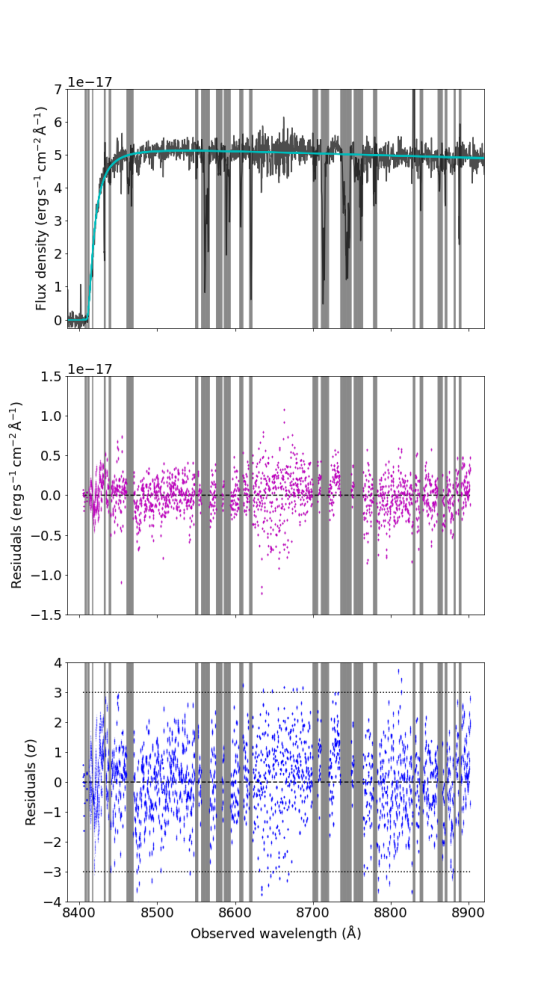
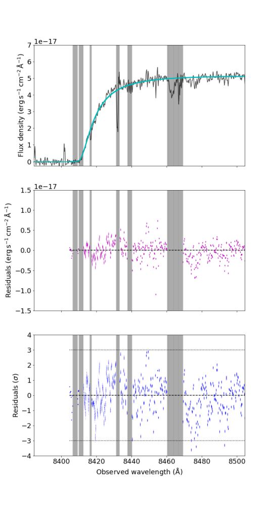
Figure 1: Example fit to the X-shooter spectrum of GRB1̃30606A using the assumptions from (Chornock et al., 2013), and $z_{\rm IGM,l}=5.8$ (left) along with a zoomed-in examination of the damping wing fit and residuals (right). Regions with metal or telluric lines are shaded grey and excluded from the fit. Top: Spectral data (black) with the 100 final positions of each walker (blue). Middle: Residual plot in $\mathrm{erg\,s^{-1}\,cm^{-2}\,\AA^{-1}}$. The dashed black line represents 0 flux. Bottom: Residual plot in $\mathrm{\sigma}$. The dashed and dotted lines represent 0 and 3 $\mathrm{\sigma}$, respectively.

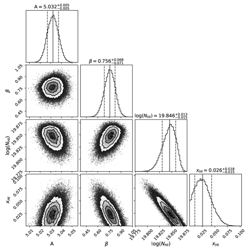
Figure 2: Posterior distribution corresponding to a fit using the assumptions from Chornock et al. (2013), with $z_{\rm IGM,l}=5.8$.

3.2.2 Totani et al. (2014) Reconstruction

While Totani et al. (2014) perform four different fits on the Subaru FOCAS spectrum, we choose to focus on reproducing the two fits that include an IGM contribution. We first attempt to reproduce the Totani et al. (2014) fit with $z_{\rm IGM,u}=z_{\rm hsost}$, and $z_{\rm IGM,l}=5.67$. When we allow the spectral index to vary freely, we find a column density of $\log(N_{\rm H}/\text{cm}^{-2})=19.47^{+0.13}_{-0.21}$ and $x_{\rm H_{I}}=0.23\pm 0.05$, (as compared to $x_{\rm H_{I}}=0.08^{+0.012}_{-0.011}$). While this value is higher than the one found by Totani et al. (2014), we agree that these assumptions lead to a positive neutral fraction detection, and the two values are within 3$\sigma$ of each other. However, the spectral index is unusually low at $\beta=0.23\pm 0.12$ (see Figure 3: Left), which is also inconsistent with the Totani et al. (2014) fit.

If we implement a Gaussian prior following the Totani et al. (2014) spectral index for this fit ($\beta=0.94\pm 0.04$), with the likelihood fixed to zero outside of the 3$\sigma$ range, the neutral fraction no longer significantly deviates from zero, with a peak at $x_{\rm H_{I}}\sim 0.01$ and a 3$\sigma$ upper limit of $x_{H_{I}}\sim 0.08$. This value is also not consistent with the original Totani et al. (2014) value of $0.086^{+0.012}_{-0.011}$.

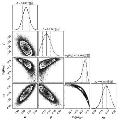
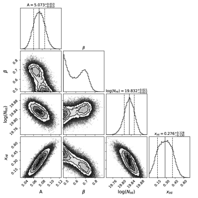
Figure 3: Posteriors for the Totani et al. (2014) results reconstruction. Left: Results reconstruction for $z_{\rm IGM,u}=z_{\rm host}$, and a free spectral index. Right: Results reconstruction for $z_{\rm IGM,u}=5.83$, and a Gaussian spectral index prior.

When we attempt to reproduce the fit using $z_{\rm IGM,u}=5.83$, we find a higher neutral fraction than the previous fit, with $x_{\rm H_{I}}=0.79^{+0.11}_{-0.14}$. It is also significantly higher than the Totani et al. (2014) result ($0.47^{+0.08}_{-0.07}$). This fit also results in a most likely spectral index of 0 with a 3$\sigma$ upper limit of $\beta<0.47$, which is unusually low (Li et al., 2015). When we implement a Gaussian spectral index prior according to the Totani et al. (2014) spectral index ($\beta=074\pm 0.09$) with the likelihood set to zero outside of the 3$\sigma$ range, we instead find a neutral fraction of $x_{\rm H_{I}}=0.28\pm 0.13$, which is lower that the Totani et al. (2014) result, but still within 3$\sigma$ (see Figure 3: Right). We note that the posterior distribution for the spectral index displays a bimodal distribution, with a small peak around $\beta\sim 0.7$, and a large peak at the boundary of the spectral index prior ($\beta\sim 0.47$). The spectral index in this fit also appears to have an anti-correlation with neutral fraction, with spectral indices around $\beta\sim 0.7$ resulting in an neutral fraction of $x_{\rm H_{I}}\sim 0.15$, and spectral indices around $\sim 0.5$ resulting in a spectral index closer to $\sim 0.4$. However, this anti-correlation is expected as a smaller spectral index requires a stronger absorption to create the same shape of damping wing.

It is important to note that the Totani et al. (2014) data range often results in a poor fit of the damping wing (see Figure 4). This can be explained by the fact that the majority of the damping wing data is not included in the fit. The omission of the damping wing could also be the cause of the volatility of the spectral index and neutral fraction result. Such a limited range of data affected by the neutral fraction can lead to a wide spread of damping wing profiles (see Figure 4: Right), and a small change in spectral index could have a large impact on the neutral fraction result.

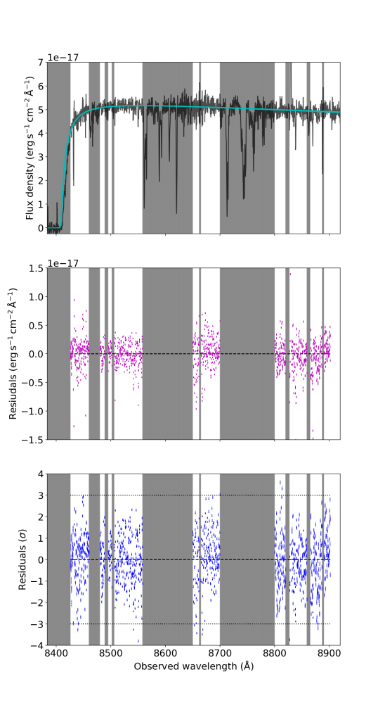
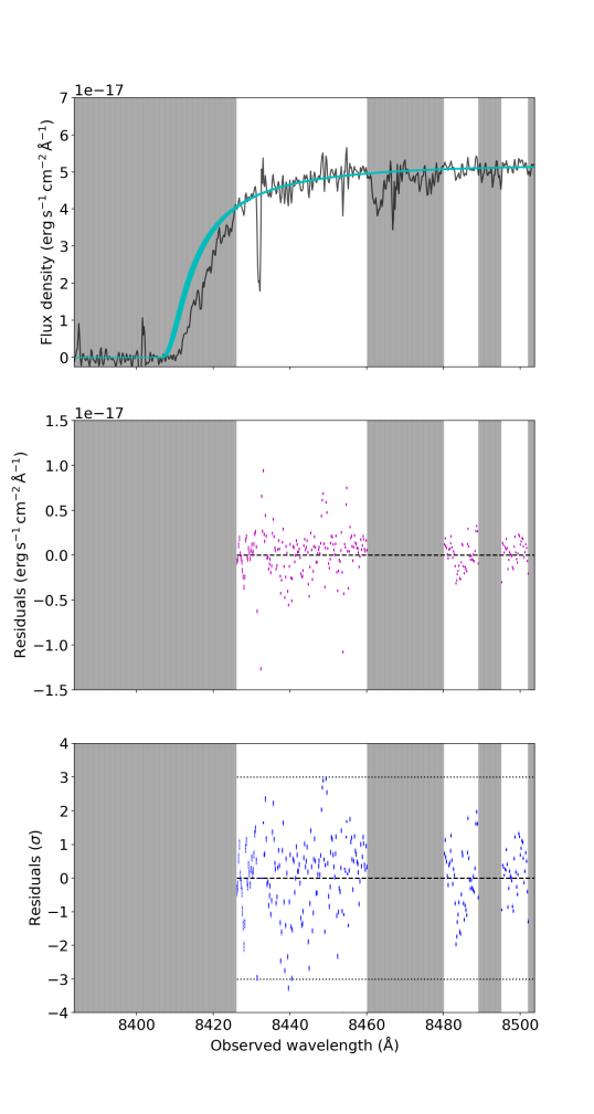
Figure 4: Left: Example fit to the X-shooter spectrum of GRB1̃30606A using the assumptions from the Totani et al. (2014) fit using $z_{\rm IGM,u}=z_{\rm host}$. Right: A zoomed-in examination of the damping wing fit and residuals. See Figure 1 for panel descriptions, and Section 3.2.2 for a discussion of the poor fit to the damping wing in this case.

3.2.3 Hartoog et al. (2015) reconstruction

When using the assumptions from Hartoog et al. (2015), we find a column density of $\log(N_{\rm H}/\text{cm}^{-2})=19.91\pm 0.01$ and neutral fraction 3$\sigma$ upper limit of $x_{\rm H_{I}}\lesssim 0.07$ (see Figure 5). Both the column density and neutral fraction are consistent with the original Hartoog et al. (2015) result.

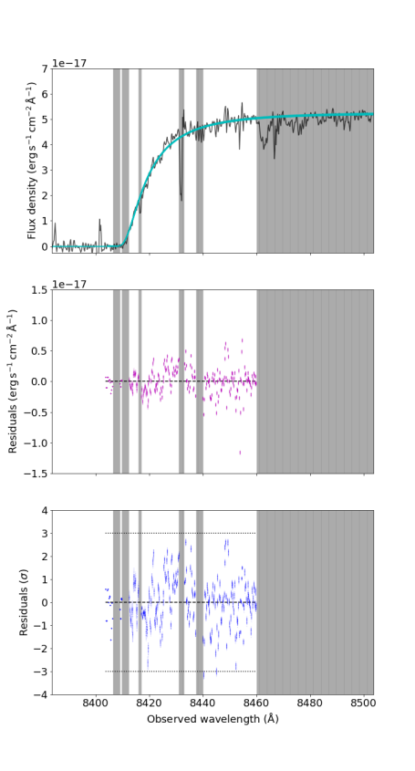
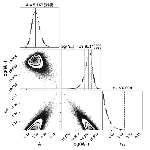
Figure 5: Left: Zoomed-in fit of the X-shooter spectrum of GRB 130606A using the assumptions from the Hartoog et al. (2015). See Figure 1 for panel descriptions. Right: Associated posteriors for the Hartoog et al. (2015) reconstruction. See Figure 1 for panel descriptions.

3.2.4 Totani et al. (2016) reconstruction

Following the neutral fraction result from Hartoog et al. (2015), Totani et al. (2016) performed a reanalysis of both the Subaru FOCAS and VLT X-shooter spectra using the assumptions from the Hartoog et al. (2015) analysis ($z_{\rm IGM,u}=5.8$, fixed spectral index of $\beta=1.02$), but with the same data ranges a the Totani et al. (2014) analysis (omission of data below 8426Å). Using these assumptions and the X-shooter data, we find a column density of $\log(N_{\rm H}/\text{cm}^{-2})=19.73\pm 0.06$ and $x_{\rm H_{I}}=0.07\pm 0.03$ (see Figure 6). This result is similar to the Totani et al. (2016) FOCAS and X-shooter neutral fraction results ($x_{\rm H_{I}}=0.061\pm 0.007$ and $x_{\rm H_{I}}=0.087^{+0.017}_{-0.029}$, respectively). The column density is also consistent with those from the Totani et al. (2016) fits.

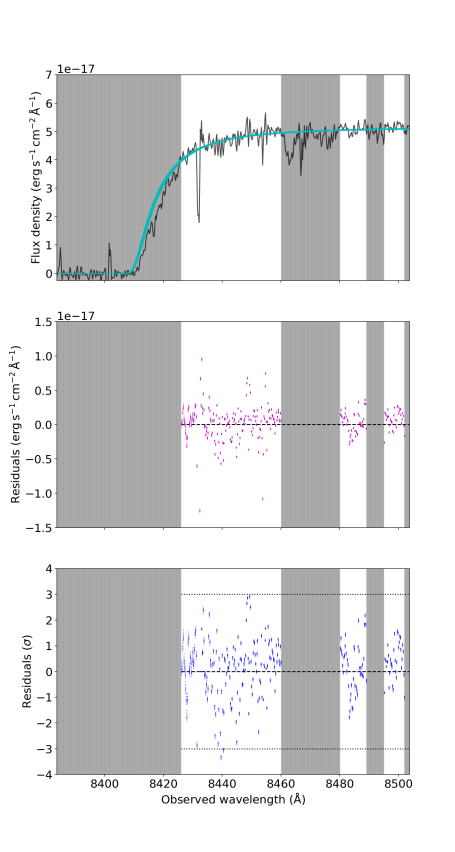
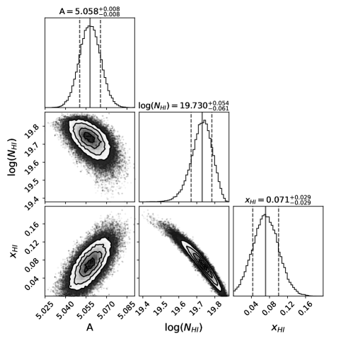
Figure 6: Left: Zoomed-in fit of the X-shooter spectrum of GRB 130606A using the assumptions from the Totani et al. (2016). See Figure 1 for panel descriptions. Right: Associated posteriors for the Totani et al. (2016) reconstruction. See Figure 1 for panel descriptions.

4 New analysis with updated models and assumptions

Most results from previous analyses can be reproduced using only the X-shooter data and each paper’s assumptions, which suggests that the main source of the discrepancies in results from the different papers stems from the assumptions each paper made in their respective analyses. It is therefore important to carefully examine what assumptions we choose and how they impact the neutral fraction result. Here we present a new analysis using the Miralda-Escude (1998) and Totani et al. (2006) models using motivated assumptions from the previous analyses. We also explore the neutral fraction result when using more realistic models that better account for the patchiness of the EoR.

4.1 Miralda-Escude (1998) methodology

We first perform an analysis using the original Miralda-Escude (1998) model. We allow the spectral index to vary freely, and use the GRB redshift estimate from the X-shooter analysis ($z_{\rm GRB}=5.91285$; Hartoog et al., 2015) since it provides the highest resolution spectrum of GRB130606A ($\sim 0.2\text{\AA}$ for the X-shooter VIS spectra as compared to $\sim 1.38\text{\AA}$ for Gemini GMOS and $\sim 0.74\text{\AA}$ for Subaru FOCAS). We fit the VLT X-shooter spectrum from $8403.74-8902$ Å  to include both the Ly$\alpha$ damping wing and a long wavelength lever arm to help constrain the continuum spectral index. When assuming $z_{\rm IGM,u}=z_{\rm GRB}$ and $z_{\rm IGM,l}=5.75$, we find a 3$\sigma$ upper limit of $x_{\rm H_{I}}\lesssim 0.04$ with a column density of $N_{\rm H_{I}}\sim 19.91\pm 0.01$, which is consistent with the column densities found in the Chornock et al. (2013) and Hartoog et al. (2015) analyses. We find a spectral index of $\beta=0.63\pm 0.06$. This is consistent with estimates from an optical-to-near-infrared spectral energy distribution using GROND data, which suggest a spectral index of $\beta\sim 0.7$ (Afonso et al., 2013). This spectral index is also consistent with results from the Swift-XRT spectrum repository, which reports an X-ray photon index of $\Gamma=1.71^{+0.11}_{-0.10}$ (90% uncertainties (Evans et al., 2007, 2009)) where $n(E)dE\propto E^{-\Gamma}$. This photon index corresponds to a spectral index with 1$\sigma$ uncertainty of $\beta=0.71\pm 0.07$, which means that there is no spectral break between the X-ray and optical regimes, as suggested in Hartoog et al. (2015).

We also perform a fit with with $z_{\rm IGM,u}=5.8$ and $z_{\rm IGM,l}=5.65$ to examine the dark trough in Ly$\alpha$ forest emission identified in Chornock et al. (2013), as was done in the Totani et al. (2014) analysis. In this case we find a neutral fraction of $x_{\rm H_{I}}\lesssim 0.53$ with a column density of $N_{\rm H_{I}}=19.91\pm 0.01$. The upper limit on the neutral fraction increases significantly, which may indicate some presence of neutral hydrogen in the system around $z\sim 5.8$. However this increase is likely partially due to the increased distance between $z_{\rm IGM,u}$ and $z_{\rm host}$, since neutral hydrogen at a redshift further from the source has a less discernible impact on the Ly$\alpha$ damping wing. We also note that the spectral index estimate for this case is a bit low with $\beta=0.57^{+0.08}_{-0.10}$.

If we use the Swift-XRT photon index estimate to implement a Gaussian spectral index prior of $\beta=0.71\pm 0.07$ with likelihood set to zero outside of the 3$\sigma$ range, we instead find a 3$\sigma$ upper limit of $x_{\rm H_{I}}\lesssim 0.23$, with a column density of $N_{\rm H_{I}}=19.91\pm 0.01$ and spectral index of $\beta=0.69^{+0.03}_{-0.04}$ (see Figure 7). This neutral fraction upper limit is still higher than the one found by using $z_{\rm IGM,u}=z_{\rm host}$, but provides a tighter constraint than the one found using a uniform spectral index prior and $z_{\rm IGM,u}=5.8$. We also note that the log-marginal-likelihood for this case is slightly better than the others. The log Bayes factor for comparing model 1 to model 0 is defined as $\ln(B_{10})=\ln(ML_{1})-\ln(ML_{0})$. According to Kass & Raftery (1995), a Bayes factor of $6<2\ln(B_{10})<10$ is strong evidence in favor of model 1, and $2\ln(B_{10})>10$ is very strong evidence in favor of model 1. From the marginal likelihood values in Table 2, we find that the model using $z_{\rm IGM,u}=5.8$ and a Gaussian spectral index prior has strong evidence ($2\ln(B_{10})=8.8$) when compared to the model with $z_{\rm IGM,u}=z_{\rm host}$ and a uniform beta prior, and very strong evidence ($2\ln(B_{10})=15.0$) when compared to the model with $z_{\rm IGM,u}=5.8$ and a uniform beta prior. This finding is consistent with results from Totani et al. (2014), who found a best fit value of $z_{IGM,u}=5.83$ through a comparison of $\chi^{2}$ values.

$z_{\rm IGM,u}$	$\beta$ prior	$\beta$ result	$x_{\rm H_{I}}$ result	$\chi^{2}$	red. $\chi^{2}$	$\ln(ML)$
$z_{\rm host}$	uniform	$0.63\pm 0.06$	$<0.04$	2714.4	1.52	-1362.1
5.8	uniform	$0.57^{+0.08}_{-0.10}$	$<0.53$	2723.2	1.53	-1365.2
5.8	Gaussian	$0.69^{+0.03}_{-0.04}$	$<0.23$	2714.7	1.52	-1357.7

Table 2: Comparison of the $\chi^{2}$, reduced $\chi^{2}$ and log-marginal-likelihoods of each new result using the Miralda-Escude (1998) model. The $\chi^{2}$ and reduced $\chi^{2}$ values for $z_{\rm IGM,u}=z_{\rm host}$ with a uniform $\beta$ prior and $z_{\rm IGM,u}=5.8$ with a Gaussian $\beta$ prior are the same. However, the marginal likelihood for $z_{\rm IGM,u}=5.8$ and a Gaussian $\beta$ prior is slightly higher than the others.

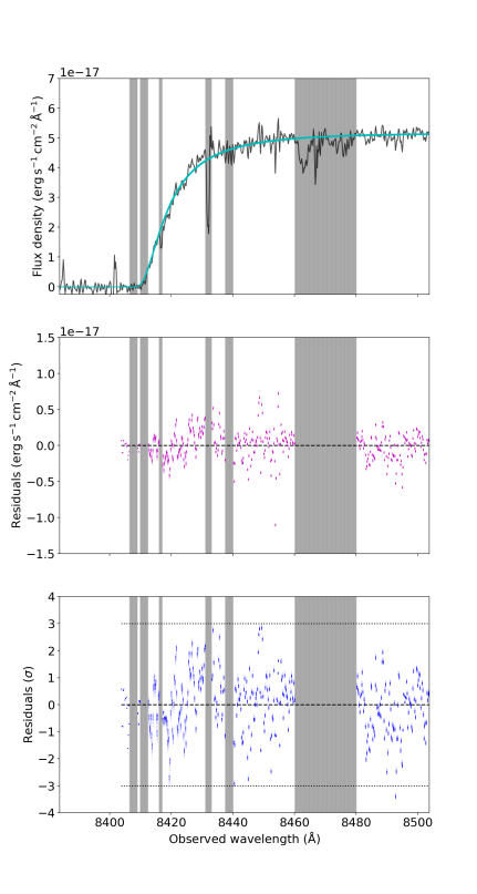
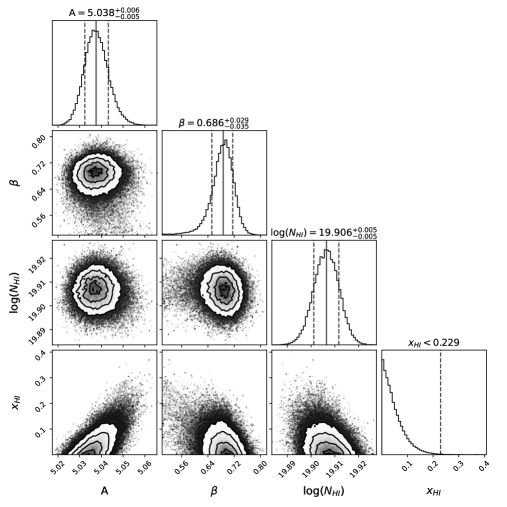
Figure 7: Posteriors for the Miralda-Escude (1998) model with $z_{\rm IGM,u}=5.8$, and $z_{\rm IGM,l}=5.65$ and a Gaussian spectral index prior.

4.2 McQuinn et al. (2008) methodology

We also analyze the spectrum using the McQuinn et al. (2008) model, which is an approximation of the Miralda-Escude (1998) model but includes a parameter for the size of an ionized bubble around the host galaxy, $R_{b}$, rather than using the assumed $z_{\rm IGM,u}$ and $z_{\rm IGM,l}$ values. We first perform a fit with $R_{b}$ as a free parameter with a uniform prior between $0\leq R_{b}\leq 60~\text{Mpc}~h^{-1}$ (or $\sim 90~\text{Mpc}$), as is predicted for ionized bubble size for a largely ionized ($x_{\rm H_{I}}\sim 0.05)$ IGM (Lidz et al., 2021). In this case, we find a neutral fraction 3$\sigma$ upper limit of $x_{\rm HI}\lesssim 0.76$, with an unconstrained bubble radius that tends towards $\sim 60~\text{Mpc}~h^{-1}$, indicating a large ionized bubble around the host galaxy. The column density ($\log(N_{\rm H_{I}}/\text{cm}^{-2})\sim 19.91$) is consistent with other results, but the spectral index is lower than expected ($\beta=0.52^{+0.11}_{-0.16}$).

If we again use a Gaussian prior for the spectral index according to the Swift-XRT photon index estimate ($\beta=0.71\pm 0.07$, with likelihood fixed to zero outside of the 3$\sigma$ range), we instead find a neutral fraction 3$\sigma$ upper limit of $x_{\rm H_{I}}\lesssim 0.20$. The bubble radius is still unconstrained but tends toward $\sim 60~\text{Mpc}~h^{-1}$, and the column density and spectral index results are consistent with those found in previous analyses (see Figure 8). The McQuinn et al. (2008) fit with a Gaussian spectral index prior has a slightly lower $\chi^{2}$ value, and has strong evidence in its favor when comparing the marginal likelihoods of the Gaussian and uniform spectral index prior results ($2\ln(B_{10})\sim 6.0$; see Table 3). The Gaussian spectral index prior was also strongly preferred for the Miralda-Escude (1998) model, which had a similar neutral fraction upper limit of $x_{\rm H_{I}}\lesssim 0.23$.

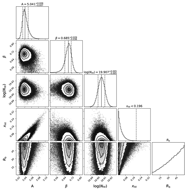
Figure 8: Posterior distributions associated with the McQuinn et al. (2008) model, a Gaussian spectral index prior, and an $R_{b}$ upper limit of $60~\text{Mpc}~h^{-1}$ or $\sim 90~\text{Mpc}$.

$\beta$ prior	$\beta$ result	$x_{\rm H_{I}}$ result	$\chi^{2}$	red. $\chi^{2}$	$\ln(ML)$
Uniform	$0.52^{+0.11}_{-0.16}$	$<0.76$	2730.8	1.53	-1358.8
Gaussian	$0.69^{+0.03}_{-0.4}$	$<0.20$	2716.4	1.52	-1355.8

Table 3: Comparison of the $\chi^{2}$, reduced $\chi^{2}$ and log-marginal-likelihoods of each new result using the McQuinn et al. (2008) model. The Gaussian prior model is strongly preferred when comparing the marginal likelihoods of the two models.

4.3 Shell implementation of the Miralda-Escude (1998) model

To better account for the patchiness of the EoR, we also use a shell implementation of the Miralda-Escude (1998) model. We first attempt fits with independent neutral fraction parameters for each shell. We use four shells with widths of $\Delta z\sim 0.1$ (or $\sim 7$ proper Mpc) starting at the GRB redshift and ending at $z\sim 5.5$. We find that for all shells the neutral fraction does not deviate significantly from 0, but the upper limit on $x_{\rm H_{I}}$ increases for shells further from the GRB host galaxy. This behavior was also observed in the analysis of GRB 210905A (Fausey et al., 2024). This effect is attributed to neutral hydrogen in the IGM having a diminishing impact on the shape of the Ly$\alpha$ damping wing the farther it is from the GRB. We find $x_{\rm H_{I}}\lesssim 0.03$ between $z=5.91285-5.8$, $x_{\rm H_{I}}\lesssim 0.51$ for $z=5.8-5.7$, and an unconstrained neutral fraction for all other shells.

We also perform fits for which the neutral fraction in each shell is coupled with a slope for the neutral fraction as a function of redshift, $dx_{H_{I}}/dz$. For these fits, the neutral fraction in the closest shell, $x_{\rm H_{I},0}$, and the slope are both treated as free parameters, and the neutral fraction values in the other shells are determined by these two parameters. We assume four shells of width $\Delta z=0.1$.

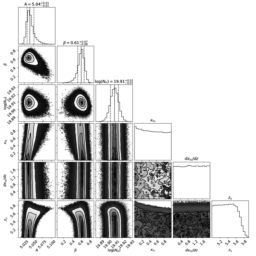
Figure 10: Posteriors for the dependent shell implementation of the Miralda-Escude (1998) model for shells of width $\Delta 0.1$ and $z_{\rm IGM,u}$ treated as a free parameter. $z_{\rm IGM,u}$ tends towards farther redshifts indicating a large ionized bubble around the GRB host galaxy. The neutral fraction, and the slope of the neutral fraction with redshift, are unconstrained.

To account for an ionized bubble, we first allow $z_{\rm IGM,u}$, the upper redshift boundary of the nearest shell to the GRB redshift, to vary as a free parameter. $z_{\rm IGM,u}$ is given a uniform prior between $5<z_{\rm IGM,u}<z_{\rm host}$. We find that when $z_{\rm IGM,u}$ is treated as a free parameter, it tends toward lower redshift, with a flat distribution between $z\sim 5.0-5.6$ that drops off at higher redshifts. This distribution indicates a large ionized bubble around the GRB host galaxy. The flat distribution for $z<5.6$ is likely because beyond this redshift neutral hydrogen no longer has any impact on the damping wing shape, so there is no way to distinguish between the effects of the choice of these redshifts (see Figure 10). For this fit, both the neutral fraction and slope of the neutral fraction as a function of redshift are also unconstrained, with a flat posterior distribution across their allowed ranges. This is likely because $z_{\rm IGM,u}$ tends towards redshifts where the IGM no longer impacts the shape of the damping wing.

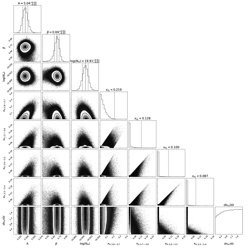
Figure 11: Posteriors for the dependent shell implementation of the Miralda-Escude (1998) model for shells of width $\Delta 0.1$, $z_{\rm IGM,u}=5.8$ and a Gaussian spectral index prior ($\mu=0.71$, $\sigma=0.07$). $x_{\rm H_{I}}$ does not significantly deviate from 0 for all shells, and the slope of the neutral fraction as a function of redshift is unconstrained. The correlation between the posteriors of the neutral fractions in different shells is due to the coupling between them according to slope $dx_{\rm H_{I}}/dz$.

We also perform fits with $z_{\rm IGM,u}$ fixed to a range of values between $z=5.85$ and $z=5.70$. All fits still use four shells of width $\Delta z=0.1$, but with the start of the first shell at different redshifts. In all cases, the neutral fraction does not deviate significantly from zero, but the upper limit on $x_{\rm H_{I}}$ in the nearest neutral shell to the GRB increases as $z_{\rm IGM,u}$ decreases. This behavior was also seen for the independent shell implementation. However, now that the neutral fraction of each shell is coupled according to some slope $dx_{\rm H_{I}}/dz$, within each individual fit the upper limit in farther shells decreases with redshift. For example, for $z_{\rm IGM,u}=5.8$, we find $x_{\rm H_{I}}\lesssim 0.48$ for $z=5.8-5.7$, $x_{\rm H_{I}}\lesssim 0.38$ for $z=5.7-5.6$, $x_{\rm H_{I}}\lesssim 0.34$ for $z=5.6-5.5$, and $x_{\rm H_{I}}\lesssim 0.31$ for $z=5.5-5.4$. The neutral fraction estimate in the highest redshift shell ($z=5.8-5.7$) is also consistent with the results when using the original Miralda-Escude (1998) model with $z_{\rm IGM,u}$. When implementing the same Gaussian spectral index prior from Sections 4.1 and 4.2, the neutral fraction upper limits in each shell also decrease, as they did for the original Miralda-Escude (1998) model (see Figure 11) with $x_{\rm H_{I}}\lesssim 0.22$ for $z=5.8-5.7$, $x_{\rm H_{I}}\lesssim 0.13$ for $z=5.7-5.6$, $x_{\rm H_{I}}\lesssim 0.10$ for $z=5.6-5.5$, and $x_{\rm H_{I}}\lesssim 0.09$ for $z=5.5-5.4$. For the dependent shell model with $z_{\rm IGM,u}=5.8$, we find strong evidence in favor of the fit using a Gaussian prior (see Table 4), which gives a 3$\sigma$ neutral fraction upper limit of $x_{\rm H_{I}}\lesssim 0.22$, and is consistent with findings of the statistically preferred fits from the Miralda-Escude (1998) and McQuinn et al. (2008) models (see Sections 4.1 and 4.2).

$\beta$ prior	$\beta$ result	$x_{\rm H_{I},z=5.8-5.7}$ result	$\chi^{2}$	red. $\chi^{2}$	$\ln(ML)$
Uniform	$0.58\pm 0.1$	$<0.48$	2720.3	1.52	-1362.1
Gaussian	$0.69\pm 0.03$	$<0.22$	2715.2	1.52	-1357.5

Table 4: Comparison of the $\chi^{2}$, reduced $\chi^{2}$ and log-marginal-likelihoods of each new result using the dependent shell implementation of the Miralda-Escude (1998) model. The Gaussian prior model is strongly preferred when comparing the marginal likelihoods.

For all values of $z_{\rm IGM,u}$ the slope $dx_{\rm H_{I}}/dz$ is unconstrained, which can be explained by the fact that the neutral fraction is already nearly zero, so the slope would not have an impact on lower-redshift shells. These results also point to a neutral fraction that does not significantly deviate from 0.

5 Discussion

In Section 3, we reproduced the previous results from other analyses using only the X-shooter spectrum, which points to the assumptions and data ranges being the source of the discrepant results in each paper, in agreement with the findings from the Totani et al. (2016) re-analysis. In Section 4, we perform a new analysis with assumptions based in new information and a range of models. We found that the preferred results for each model all point to a neutral fraction $3\sigma$ upper limit of $x_{H_{I}}\lesssim 0.20-0.23$. In this Section, we discuss the potential for a system at $z\sim 5.8$, compare the analysis of GRB 130606A to other GRB damping wing analyses, and explore the implications the new result in the broader context of EoR measurements and models.

5.1 Potential System at $z\sim 5.8$

The Chornock et al. (2013) analysis of GRB 130606A identified a potential DLA at $z\sim 5.8$ using metal lines, and noted that it seemed to correspond to a dark trough in Ly$\alpha$ transmission from $z\sim 5.72-5.79$. Totani et al. (2014) noted that their best fit $z_{\rm IGM,u}$ value corresponded to the same redshift as the dark trough in Ly$\alpha$ transmission. We do not find sufficient evidence for a DLA or a significant neutral fraction at $z\sim 5.7-5.8$ within the damping wing analysis. However, $z\sim 5.8$ is already $\sim 50~\text{Mpc}~h^{-1}$ from the GRB redshift. The farther away neutral hydrogen is from the GRB redshift, the higher the neutral fraction must be to have a discernable impact. It is possible that there is some neutral hydrogen around $z\sim 5.8-5.7$, but not in a high enough quantity to be effectively measured with the Ly$\alpha$ damping wing.

5.2 Comparison with Other GRB Results

For GRB 130606A, we find a 3$\sigma$ neutral fraction upper limit of $x_{\rm H_{I}}\lesssim 0.20-0.23$. This result is roughly in agreement with current EoR models and neutral fraction measurements (e.g., Ishigaki et al., 2018; Finkelstein et al., 2019; Naidu et al., 2020; Zhu et al., 2022; Jin et al., 2023; Bruton et al., 2023). However, the neutral fraction upper limit for GRB 130606A is higher than or equal to that of GRB 210905A, a $z\sim 6.3$ GRB with a 3$\sigma$ neutral fraction upper limit of $x_{\rm H_{I}}\lesssim 0.15-0.23$ (Fausey et al., 2024). There are a number of reasons that the neutral fraction upper limit for GRB 130606A may be larger than that of GRB 210905A.

Some previous analyses of GRB 130606A identified a potential DLA and/or a potentially neutral system at $z\sim 5.8$ (Chornock et al., 2013; Totani et al., 2014, see Section 5.1). While we did not find clear evidence for this potential system in our damping wing analysis, it is possible that there is neutral hydrogen between $z\sim 5.8-5.7$ in high enough quantities to drive up the neutral fraction upper limit, but not in high enough quantities to allow for a clear detection.

GRB 210905A may have had an over-ionized sightline for its redshift (Fausey et al., 2024), which could explain why it has a lower neutral fraction upper limit than GRB 130606A. This discrepancy between GRB damping wing results highlights the potential impact that the line of sight can have on a GRB neutral fraction estimate. It will be vital to increase the number of high-redshift GRBs with high-quality spectroscopic observations so that we will not have to rely on the sightlines of just a few GRBs to obtain a neutral fraction estimate at different redshifts.

5.3 Comparison with Different Methods for Estimating $x_{\rm H_{I}}$ Evolution

There are still multiple sources of uncertainty in EoR modeling. The escape fraction, $f_{esc}$, denotes the average fraction of ionizing photons that escape from the galaxies in which they are produced, and is important for understanding the evolution of the EoR. It has been measured using a variety of sources with redshifts $z\lesssim 4$ (Mostardi et al., 2015; Rutkowski et al., 2016; Vanzella et al., 2016; Steidel et al., 2018; Tanvir et al., 2019; Vielfaure et al., 2020; Izotov et al., 2021; Pahl et al., 2021), and even up to $z\sim 5$ with a GRB afterglow (Levan et al., 2024b). However, determining $f_{esc}$ at higher redshifts is increasingly difficult due to an increase in intergalactic attenuation at higher redshifts (Madau, 1995; Inoue et al., 2014; Robertson, 2022). While studies have been done to indirectly estimate the escape fraction at higher redshifts (i.e., Kakiichi et al., 2018; Tanvir et al., 2019; Meyer et al., 2020), more work is required for a complete understanding of the escape fraction at different redshifts (Robertson, 2022). The UV luminosity function is another key component of reionization models that describes the distribution of galaxy UV luminosities as a function of redshift (Tanvir et al., 2012). It has changed significantly with the launch of JWST, which detected more high luminosities galaxies at high redshifts than previously expected (Finkelstein et al., 2023; Harikane et al., 2023; Muñoz et al., 2024), which could have impacted the early progression of the EoR (Robertson, 2022; Bruton et al., 2023). There is also still debate as to whether bright or faint galaxies are the primary sources of ionizing radiation (Naidu et al., 2020; Bruton et al., 2023; Wu & Kravtsov, 2024), and whether or not AGN also played a role (Finkelstein et al., 2019).

There are a wide range of methods and probes for estimating the neutral fraction at different redshifts. Ly$\alpha$ damping wings of quasars and Lyman Break Galaxies (LBGs) can be used to obtain neutral fraction estimate, with some additional considerations for their more complex continua, and the impact of continuous ionizing radiation from quasars (Bañados et al., 2018; Davies et al., 2018; Greig et al., 2019; Yang et al., 2020; Wang et al., 2020; Greig et al., 2022; Hsiao et al., 2023; Umeda et al., 2024). LAEs are also useful for neutral fraction estimation. LAEs are clustered in the sky rather than isotropically distributed, and the amount of clustering is expected to increase at higher redshift due to the patchiness of the IGM, since LAEs in large ionized bubbles are less impacted by Ly$\alpha$ absorption (Ouchi et al., 2018). Examining the clustering of LAEs as a function of redshift can provide insight into the neutral fraction at different redshifts (Ouchi et al., 2018). The evolution of the LAE luminosity function in comparison with the UV luminosity function can help estimate the change in Ly$\alpha$ transmission, which can be related to the neutral fraction and ionized bubble sizes (Inoue et al., 2018; Konno et al., 2018; Morales et al., 2021). Finally, the evolution of equivalent widths of LAE Ly$\alpha$ emission lines can provide insight into the evolution of the EoR (Mason et al., 2018). Dark pixels and troughs in Ly$\alpha$ and Ly$\beta$ transmission can also indicate the presence of neutral hydrogen in the IGM at different redshifts (Zhu et al., 2022; Jin et al., 2023). Recently, Zhu et al. (2024) stacked Ly$\alpha$ transmission profiles according to gaps in Ly$\beta$ transmission in search of Ly$\alpha$ damping wing features. The Planck survey also estimated the midpoint of reionization using electron scattering optical depth estimates (Planck Collaboration et al., 2020). A compilation of results from these methods of neutral fraction estimation are presented in Figure 9 along with theoretical curves for four different models (Ishigaki et al., 2018; Finkelstein et al., 2019; Naidu et al., 2020; Bruton et al., 2023). For EoR theoretical curves, we show only one line rather than the entire model ranges.

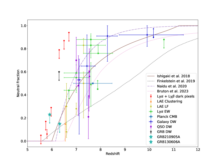
Figure 9: Recent EoR models (Ishigaki et al., 2018; Finkelstein et al., 2019; Naidu et al., 2020; Bruton et al., 2023) and neutral fraction estimates as a function of redshift using a variety of methods. The cyan stars show results from the analysis of the GRB 130606A damping wing (this paper) and the GRB 210905A damping wing (Fausey et al., 2024). Other neutral fraction results obtained from GRB damping wings are marked with a black star (GRB 050904; Totani et al., 2006). Red circles represent neutral fraction results from dark pixel fractions/troughs (Zhu et al., 2022; Jin et al., 2023); orange triangles from Lyman-$\alpha$ emitter clustering (Ouchi et al., 2018) yellow plus signs from Lyman-$\alpha$ emitter luminosity functions (Konno et al., 2018; Inoue et al., 2018; Morales et al., 2021); green squares from Lyman-$\alpha$ equivalent widths (Mason et al., 2018, 2019; Hoag et al., 2019; Whitler et al., 2020; Jung et al., 2020; Bolan et al., 2022; Bruton et al., 2023; Morishita et al., 2023); light blue cross from the Planck survey (Planck Collaboration et al., 2020); dark blue diamonds from galaxy damping wings (Hsiao et al., 2023; Umeda et al., 2024); and purple pentagons from quasar damping wings (Bañados et al., 2018; Davies et al., 2018; Greig et al., 2019; Yang et al., 2020; Wang et al., 2020; Greig et al., 2022).

There is still a large amount of uncertainty in the progression of the EoR. There are a wide range of neutral fraction estimates at each redshift, making it difficult to resolve the EoR progression. Increasing the number of neutral fraction measurement from a large range of probes will be vital to understanding the EoR and its evolution. Since GRBs fade rapidly, quick spectral follow-up can greatly improve the data quality. However, it can be difficult to quickly determine which GRBs are high redshift, as they often require near-infrared imaging for their identification. Proposed missions like the Gamow Explorer (Gamow White et al., 2021) and Transient High-Energy Sky and Early Universe Surveyor (THESEUS Amati et al., 2021) are designed to quickly identify high-redshift GRBs and alert the community, so they can aid in decreasing the time between GRB detection and observation. New missions such as Einstein Probe (Yuan et al., 2022), and the Space Variable Objects Monitor (SVOM Atteia et al., 2022) will also likely increase the sample of high redshift GRBs. Additionally, JWST (Greenhouse, 2016) and a new generation of 30-meter telescopes (Neichel et al., 2018), along with new instruments such as SCORPIO (Robberto et al., 2020) on the Gemini Telescope, will provide more high-quality optical-to-near-infrared spectra for GRB damping wing analyses, enabling better constraints on the progression of the EoR. In particular, the simultaneous channels of SCORPIO will be easier to calibrate than an instrument like X-shooter, which has curved orders and three separate arms for UV, optical, and near-infrared observations, so it may cut down on correlated noise and uncertainties in the spectrum and allow for more precise estimates of the neutral fraction.

6 Conclusions

GRBs are excellent probes of the high-redshift Universe. The Ly$\alpha$ damping wing of high-redshift GRBs can provide insight into the neutral fraction at different redshifts and track the progression of the EoR. GRB 130606A is a high-redshift GRB for which multiple analyses using data sets from different telescopes and varying assumptions found different neutral fraction results. We reproduce all results using the VLT X-shooter spectrum and the corresponding assumptions of each analysis, highlighting the notable impact that assumptions can have on neutral fraction results. We present new analyses using assumptions motivated by new insights and multiple models, to ensure the robustness of the results. For the original Miralda-Escude (1998) model, the McQuinn et al. (2008) model, and a shell implementation of the Miralda-Escude (1998) model, the statistically preferred results give a 3$\sigma$ neutral fraction upper limit of $x_{\rm H_{I}}\lesssim 0.28$, $x_{\rm H_{I}}\lesssim 0.24$, and $x_{\rm H_{I}}\lesssim 0.26$, respectively. We compare these results to the neutral fraction analysis of GRB 210905A which resides at a slightly higher redshift, and present both GRB damping wing neutral fraction estimates in the context of neutral fraction measurements from other probes and EoR models. More high-redshift GRBs will be vital for probing the EoR at different redshifts, and reducing the reliance on the lines of sight of individual GRBs.

Appendix A Shell Implementation Fits Posteriors

In this appendix, we show the posterior distribution associated with the independent and dependent shell implementations of the Miralda-Escude (1998) fit.

References

- Abbott et al. (2017) Abbott, B. P., Abbott, R., Abbott, T. D., et al. 2017, ApJ, 848, L13, doi: 10.3847/2041-8213/aa920c
- Afonso et al. (2013) Afonso, P., Kann, D. A., Nicuesa Guelbenzu, A., et al. 2013, GRB Coordinates Network, 14807, 1
- Amati et al. (2021) Amati, L., O’Brien, P. T., Götz, D., et al. 2021, Experimental Astronomy, 52, 183, doi: 10.1007/s10686-021-09807-8
- Arons & Wingert (1972) Arons, J., & Wingert, D. W. 1972, ApJ, 177, 1, doi: 10.1086/151682
- Astropy Collaboration et al. (2013) Astropy Collaboration, Robitaille, T. P., Tollerud, E. J., et al. 2013, A&A, 558, A33, doi: 10.1051/0004-6361/201322068
- Astropy Collaboration et al. (2018) Astropy Collaboration, Price-Whelan, A. M., Sipőcz, B. M., et al. 2018, AJ, 156, 123, doi: 10.3847/1538-3881/aabc4f
- Astropy Collaboration et al. (2022) Astropy Collaboration, Price-Whelan, A. M., Lim, P. L., et al. 2022, ApJ, 935, 167, doi: 10.3847/1538-4357/ac7c74
- Atteia et al. (2022) Atteia, J. L., Cordier, B., & Wei, J. 2022, International Journal of Modern Physics D, 31, 2230008, doi: 10.1142/S0218271822300087
- Bañados et al. (2018) Bañados, E., Venemans, B. P., Mazzucchelli, C., et al. 2018, Nature, 553, 473, doi: 10.1038/nature25180
- Barkana & Loeb (2004) Barkana, R., & Loeb, A. 2004, ApJ, 601, 64, doi: 10.1086/380435
- Becker & Bolton (2013) Becker, G. D., & Bolton, J. S. 2013, MNRAS, 436, 1023, doi: 10.1093/mnras/stt1610
- Beniamini & Granot (2016) Beniamini, P., & Granot, J. 2016, MNRAS, 459, 3635, doi: 10.1093/mnras/stw895
- Bolan et al. (2022) Bolan, P., Lemaux, B. C., Mason, C., et al. 2022, MNRAS, 517, 3263, doi: 10.1093/mnras/stac1963
- Bouwens et al. (2012) Bouwens, R. J., Illingworth, G. D., Oesch, P. A., et al. 2012, ApJ, 752, L5, doi: 10.1088/2041-8205/752/1/L5
- Bruton et al. (2023) Bruton, S., Lin, Y.-H., Scarlata, C., & Hayes, M. J. 2023, ApJ, 949, L40, doi: 10.3847/2041-8213/acd5d0
- Burns et al. (2023) Burns, E., Svinkin, D., Fenimore, E., et al. 2023, ApJ, 946, L31, doi: 10.3847/2041-8213/acc39c
- Campisi et al. (2011) Campisi, M. A., Maio, U., Salvaterra, R., & Ciardi, B. 2011, MNRAS, 416, 2760, doi: 10.1111/j.1365-2966.2011.19238.x
- Castro-Tirado et al. (2013) Castro-Tirado, A. J., Sánchez-Ramírez, R., Ellison, S. L., et al. 2013, arXiv e-prints, arXiv:1312.5631, doi: 10.48550/arXiv.1312.5631
- Chevalier & Li (1999) Chevalier, R. A., & Li, Z.-Y. 1999, ApJ, 520, L29, doi: 10.1086/312147
- Chornock et al. (2013) Chornock, R., Berger, E., Fox, D. B., et al. 2013, ApJ, 774, 26, doi: 10.1088/0004-637X/774/1/26
- Ciardi & Loeb (2000) Ciardi, B., & Loeb, A. 2000, ApJ, 540, 687, doi: 10.1086/309384
- Cucchiara et al. (2011) Cucchiara, A., Levan, A. J., Fox, D. B., et al. 2011, ApJ, 736, 7, doi: 10.1088/0004-637X/736/1/7
- Davies et al. (2018) Davies, F. B., Hennawi, J. F., Bañados, E., et al. 2018, ApJ, 864, 142, doi: 10.3847/1538-4357/aad6dc
- Eichler et al. (1989) Eichler, D., Livio, M., Piran, T., & Schramm, D. N. 1989, Nature, 340, 126, doi: 10.1038/340126a0
- Evans et al. (2007) Evans, P. A., Beardmore, A. P., Page, K. L., et al. 2007, A&A, 469, 379, doi: 10.1051/0004-6361:20077530
- Evans et al. (2009) —. 2009, MNRAS, 397, 1177, doi: 10.1111/j.1365-2966.2009.14913.x
- Faucher-Giguère et al. (2008) Faucher-Giguère, C.-A., Lidz, A., Hernquist, L., & Zaldarriaga, M. 2008, ApJ, 688, 85, doi: 10.1086/592289
- Fausey et al. (2024) Fausey, H. M., Vejlgaard, S., van der Horst, A. J., et al. 2024, arXiv e-prints, arXiv:2403.13126, doi: 10.48550/arXiv.2403.13126
- Finkelstein et al. (2019) Finkelstein, S. L., D’Aloisio, A., Paardekooper, J.-P., et al. 2019, ApJ, 879, 36, doi: 10.3847/1538-4357/ab1ea8
- Finkelstein et al. (2023) Finkelstein, S. L., Bagley, M. B., Ferguson, H. C., et al. 2023, ApJ, 946, L13, doi: 10.3847/2041-8213/acade4
- Foreman-Mackey (2016) Foreman-Mackey, D. 2016, The Journal of Open Source Software, 1, 24, doi: 10.21105/joss.00024
- Foreman-Mackey et al. (2013) Foreman-Mackey, D., Hogg, D. W., Lang, D., & Goodman, J. 2013, PASP, 125, 306, doi: 10.1086/670067
- Frederiks et al. (2013) Frederiks, D. D., Hurley, K., Svinkin, D. S., et al. 2013, ApJ, 779, 151, doi: 10.1088/0004-637X/779/2/151
- Fryer et al. (2022) Fryer, C. L., Lien, A. Y., Fruchter, A., et al. 2022, ApJ, 929, 111, doi: 10.3847/1538-4357/ac5d5c
- Galama et al. (1998) Galama, T. J., Vreeswijk, P. M., van Paradijs, J., et al. 1998, Nature, 395, 670, doi: 10.1038/27150
- Gao et al. (2022) Gao, H., Lei, W.-H., & Zhu, Z.-P. 2022, ApJ, 934, L12, doi: 10.3847/2041-8213/ac80c7
- Giannios & Spruit (2007) Giannios, D., & Spruit, H. C. 2007, A&A, 469, 1, doi: 10.1051/0004-6361:20066739
- Goldoni (2011) Goldoni, P. 2011, Astronomische Nachrichten, 332, 227, doi: 10.1002/asna.201111523
- Gou et al. (2004) Gou, L. J., Mészáros, P., Abel, T., & Zhang, B. 2004, ApJ, 604, 508, doi: 10.1086/382061
- Greenhouse (2016) Greenhouse, M. A. 2016, in Society of Photo-Optical Instrumentation Engineers (SPIE) Conference Series, Vol. 9904, Space Telescopes and Instrumentation 2016: Optical, Infrared, and Millimeter Wave, ed. H. A. MacEwen, G. G. Fazio, M. Lystrup, N. Batalha, N. Siegler, & E. C. Tong, 990406, doi: 10.1117/12.2231448
- Greig et al. (2019) Greig, B., Mesinger, A., & Bañados, E. 2019, MNRAS, 484, 5094, doi: 10.1093/mnras/stz230
- Greig et al. (2022) Greig, B., Mesinger, A., Davies, F. B., et al. 2022, MNRAS, 512, 5390, doi: 10.1093/mnras/stac825
- Harikane et al. (2023) Harikane, Y., Ouchi, M., Oguri, M., et al. 2023, ApJS, 265, 5, doi: 10.3847/1538-4365/acaaa9
- Hartoog et al. (2015) Hartoog, O. E., Malesani, D., Fynbo, J. P. U., et al. 2015, A&A, 580, A139, doi: 10.1051/0004-6361/201425001
- Hjorth et al. (2003) Hjorth, J., Sollerman, J., Møller, P., et al. 2003, Nature, 423, 847, doi: 10.1038/nature01750
- Hoag et al. (2019) Hoag, A., Bradač, M., Huang, K., et al. 2019, ApJ, 878, 12, doi: 10.3847/1538-4357/ab1de7
- Hook et al. (2004) Hook, I. M., Jørgensen, I., Allington-Smith, J. R., et al. 2004, PASP, 116, 425, doi: 10.1086/383624
- Hsiao et al. (2023) Hsiao, T. Y.-Y., Abdurro’uf, Coe, D., et al. 2023, arXiv e-prints, arXiv:2305.03042, doi: 10.48550/arXiv.2305.03042
- Inoue et al. (2014) Inoue, A. K., Shimizu, I., Iwata, I., & Tanaka, M. 2014, MNRAS, 442, 1805, doi: 10.1093/mnras/stu936
- Inoue et al. (2018) Inoue, A. K., Hasegawa, K., Ishiyama, T., et al. 2018, PASJ, 70, 55, doi: 10.1093/pasj/psy048
- Ishigaki et al. (2018) Ishigaki, M., Kawamata, R., Ouchi, M., et al. 2018, ApJ, 854, 73, doi: 10.3847/1538-4357/aaa544
- Izotov et al. (2021) Izotov, Y. I., Worseck, G., Schaerer, D., et al. 2021, MNRAS, 503, 1734, doi: 10.1093/mnras/stab612
- Jin et al. (2023) Jin, X., Yang, J., Fan, X., et al. 2023, ApJ, 942, 59, doi: 10.3847/1538-4357/aca678
- Jones et al. (2013) Jones, A., Noll, S., Kausch, W., Szyszka, C., & Kimeswenger, S. 2013, A&A, 560, A91, doi: 10.1051/0004-6361/201322433
- Jung et al. (2020) Jung, I., Finkelstein, S. L., Dickinson, M., et al. 2020, ApJ, 904, 144, doi: 10.3847/1538-4357/abbd44
- Kakiichi et al. (2018) Kakiichi, K., Ellis, R. S., Laporte, N., et al. 2018, MNRAS, 479, 43, doi: 10.1093/mnras/sty1318
- Kashikawa et al. (2002) Kashikawa, N., Aoki, K., Asai, R., et al. 2002, PASJ, 54, 819, doi: 10.1093/pasj/54.6.819
- Kass & Raftery (1995) Kass, R. E., & Raftery, A. E. 1995, Journal of the American Statistical Association, 90, 773, doi: 10.1080/01621459.1995.10476572
- Konno et al. (2018) Konno, A., Ouchi, M., Shibuya, T., et al. 2018, PASJ, 70, S16, doi: 10.1093/pasj/psx131
- Kouveliotou et al. (1993) Kouveliotou, C., Meegan, C. A., Fishman, G. J., et al. 1993, ApJ, 413, L101, doi: 10.1086/186969
- Lamb & Reichart (2000) Lamb, D. Q., & Reichart, D. E. 2000, The Astrophysical Journal, 536, 1, doi: 10.1086/308918
- Levan et al. (2024a) Levan, A. J., Gompertz, B. P., Salafia, O. S., et al. 2024a, Nature, 626, 737, doi: 10.1038/s41586-023-06759-1
- Levan et al. (2024b) Levan, A. J., Jonker, P. G., Saccardi, A., et al. 2024b, arXiv e-prints, arXiv:2404.16350, doi: 10.48550/arXiv.2404.16350
- Li et al. (2015) Li, L., Wu, X.-F., Huang, Y.-F., et al. 2015, ApJ, 805, 13, doi: 10.1088/0004-637X/805/1/13
- Lidz et al. (2021) Lidz, A., Chang, T.-C., Mas-Ribas, L., & Sun, G. 2021, ApJ, 917, 58, doi: 10.3847/1538-4357/ac0af0
- Lloyd-Ronning et al. (2002) Lloyd-Ronning, N. M., Fryer, C. L., & Ramirez-Ruiz, E. 2002, ApJ, 574, 554, doi: 10.1086/341059
- Lyubarsky (2010) Lyubarsky, Y. 2010, The Astrophysical Journal Letters, 725, L234, doi: 10.1088/2041-8205/725/2/L234
- Madau (1995) Madau, P. 1995, ApJ, 441, 18, doi: 10.1086/175332
- Mason et al. (2018) Mason, C. A., Treu, T., Dijkstra, M., et al. 2018, ApJ, 856, 2, doi: 10.3847/1538-4357/aab0a7
- Mason et al. (2019) Mason, C. A., Fontana, A., Treu, T., et al. 2019, MNRAS, 485, 3947, doi: 10.1093/mnras/stz632
- Matthee et al. (2023) Matthee, J., Naidu, R. P., Brammer, G., et al. 2023, arXiv e-prints, arXiv:2306.05448, doi: 10.48550/arXiv.2306.05448
- Mazets et al. (1981) Mazets, E. P., Golenetskii, S. V., Ilinskii, V. N., et al. 1981, Ap&SS, 80, 3, doi: 10.1007/BF00649140
- McEwen et al. (2021) McEwen, J. D., Wallis, C. G. R., Price, M. A., & Docherty, M. M. 2021, arXiv e-prints, arXiv:2111.12720, doi: 10.48550/arXiv.2111.12720
- McQuinn (2016) McQuinn, M. 2016, ARA&A, 54, 313, doi: 10.1146/annurev-astro-082214-122355
- McQuinn et al. (2008) McQuinn, M., Lidz, A., Zaldarriaga, M., Hernquist, L., & Dutta, S. 2008, MNRAS, 388, 1101, doi: 10.1111/j.1365-2966.2008.13271.x
- Melandri et al. (2015) Melandri, A., Bernardini, M. G., D’Avanzo, P., et al. 2015, A&A, 581, A86, doi: 10.1051/0004-6361/201526660
- Meyer et al. (2020) Meyer, R. A., Kakiichi, K., Bosman, S. E. I., et al. 2020, MNRAS, 494, 1560, doi: 10.1093/mnras/staa746
- Miralda-Escude (1998) Miralda-Escude, J. 1998, The Astrophysical Journal, 501, 15, doi: 10.1086/305799
- Morales et al. (2021) Morales, A. M., Mason, C. A., Bruton, S., et al. 2021, ApJ, 919, 120, doi: 10.3847/1538-4357/ac1104
- Morishita et al. (2023) Morishita, T., Roberts-Borsani, G., Treu, T., et al. 2023, ApJ, 947, L24, doi: 10.3847/2041-8213/acb99e
- Mostardi et al. (2015) Mostardi, R. E., Shapley, A. E., Steidel, C. C., et al. 2015, ApJ, 810, 107, doi: 10.1088/0004-637X/810/2/107
- Muñoz et al. (2024) Muñoz, J. B., Mirocha, J., Chisholm, J., Furlanetto, S. R., & Mason, C. 2024, MNRAS, 535, L37, doi: 10.1093/mnrasl/slae086
- Naidu et al. (2020) Naidu, R. P., Tacchella, S., Mason, C. A., et al. 2020, ApJ, 892, 109, doi: 10.3847/1538-4357/ab7cc9
- Narayan et al. (1992) Narayan, R., Paczynski, B., & Piran, T. 1992, ApJ, 395, L83, doi: 10.1086/186493
- Neichel et al. (2018) Neichel, B., Mouillet, D., Gendron, E., et al. 2018, in SF2A-2018: Proceedings of the Annual meeting of the French Society of Astronomy and Astrophysics, ed. P. Di Matteo, F. Billebaud, F. Herpin, N. Lagarde, J. B. Marquette, A. Robin, & O. Venot, Di, doi: 10.48550/arXiv.1812.06639
- Noll et al. (2012) Noll, S., Kausch, W., Barden, M., et al. 2012, A&A, 543, A92, doi: 10.1051/0004-6361/201219040
- Ouchi et al. (2018) Ouchi, M., Harikane, Y., Shibuya, T., et al. 2018, PASJ, 70, S13, doi: 10.1093/pasj/psx074
- Pahl et al. (2021) Pahl, A. J., Shapley, A., Steidel, C. C., Chen, Y., & Reddy, N. A. 2021, MNRAS, 505, 2447, doi: 10.1093/mnras/stab1374
- Patel et al. (2010) Patel, M., Warren, S. J., Mortlock, D. J., & Fynbo, J. P. U. 2010, A&A, 512, L3, doi: 10.1051/0004-6361/200913876
- Planck Collaboration et al. (2020) Planck Collaboration, Aghanim, N., Akrami, Y., et al. 2020, A&A, 641, A6, doi: 10.1051/0004-6361/201833910
- Qin et al. (2021) Qin, Y., Mesinger, A., Bosman, S. E. I., & Viel, M. 2021, MNRAS, 506, 2390, doi: 10.1093/mnras/stab1833
- Rastinejad et al. (2022) Rastinejad, J. C., Gompertz, B. P., Levan, A. J., et al. 2022, Nature, 612, 223, doi: 10.1038/s41586-022-05390-w
- Rees & Meszaros (1992) Rees, M. J., & Meszaros, P. 1992, MNRAS, 258, 41, doi: 10.1093/mnras/258.1.41P
- Robberto et al. (2020) Robberto, M., Roming, P. W. A., van der Horst, A. J., et al. 2020, in Society of Photo-Optical Instrumentation Engineers (SPIE) Conference Series, Vol. 11447, Society of Photo-Optical Instrumentation Engineers (SPIE) Conference Series, 1144774, doi: 10.1117/12.2568031
- Robertson (2022) Robertson, B. E. 2022, ARA&A, 60, 121, doi: 10.1146/annurev-astro-120221-044656
- Robertson et al. (2015) Robertson, B. E., Ellis, R. S., Furlanetto, S. R., & Dunlop, J. S. 2015, ApJ, 802, L19, doi: 10.1088/2041-8205/802/2/L19
- Rossi et al. (2022) Rossi, A., Rothberg, B., Palazzi, E., et al. 2022, ApJ, 932, 1, doi: 10.3847/1538-4357/ac60a2
- Rutkowski et al. (2016) Rutkowski, M. J., Scarlata, C., Haardt, F., et al. 2016, ApJ, 819, 81, doi: 10.3847/0004-637X/819/1/81
- Saccardi et al. (2023) Saccardi, A., Vergani, S. D., De Cia, A., et al. 2023, A&A, 671, A84, doi: 10.1051/0004-6361/202244205
- Salvaterra (2015) Salvaterra, R. 2015, Journal of High Energy Astrophysics, 7, 35, doi: 10.1016/j.jheap.2015.03.001
- Salvaterra et al. (2009) Salvaterra, R., Della Valle, M., Campana, S., et al. 2009, Nature, 461, 1258, doi: 10.1038/nature08445
- Sari et al. (1999) Sari, R., Piran, T., & Halpern, J. P. 1999, ApJ, 519, L17, doi: 10.1086/312109
- Sari et al. (1998) Sari, R., Piran, T., & Narayan, R. 1998, The Astrophysical Journal, 497, L17, doi: 10.1086/311269
- Savaglio (2006) Savaglio, S. 2006, New Journal of Physics, 8, 195, doi: 10.1088/1367-2630/8/9/195
- Sparre et al. (2014) Sparre, M., Hartoog, O. E., Krühler, T., et al. 2014, ApJ, 785, 150, doi: 10.1088/0004-637X/785/2/150
- Spruit et al. (2001) Spruit, H. C., Daigne, F., & Drenkhahn, G. 2001, A&A, 369, 694, doi: 10.1051/0004-6361:20010131
- Steidel et al. (2018) Steidel, C. C., Bogosavljević, M., Shapley, A. E., et al. 2018, ApJ, 869, 123, doi: 10.3847/1538-4357/aaed28
- Tanvir et al. (2009) Tanvir, N. R., Fox, D. B., Levan, A. J., et al. 2009, Nature, 461, 1254, doi: 10.1038/nature08459
- Tanvir et al. (2012) Tanvir, N. R., Levan, A. J., Fruchter, A. S., et al. 2012, ApJ, 754, 46, doi: 10.1088/0004-637X/754/1/46
- Tanvir et al. (2018) Tanvir, N. R., Laskar, T., Levan, A. J., et al. 2018, ApJ, 865, 107, doi: 10.3847/1538-4357/aadba9
- Tanvir et al. (2019) Tanvir, N. R., Fynbo, J. P. U., de Ugarte Postigo, A., et al. 2019, MNRAS, 483, 5380, doi: 10.1093/mnras/sty3460
- Thompson (1994) Thompson, C. 1994, MNRAS, 270, 480, doi: 10.1093/mnras/270.3.480
- Thöne et al. (2013) Thöne, C. C., Fynbo, J. P. U., Goldoni, P., et al. 2013, MNRAS, 428, 3590, doi: 10.1093/mnras/sts303
- Totani et al. (2016) Totani, T., Aoki, K., Hattori, T., & Kawai, N. 2016, PASJ, 68, 15, doi: 10.1093/pasj/psv123
- Totani et al. (2006) Totani, T., Kawai, N., Kosugi, G., et al. 2006, PASJ, 58, 485, doi: 10.1093/pasj/58.3.485
- Totani et al. (2014) Totani, T., Aoki, K., Hattori, T., et al. 2014, PASJ, 66, 63, doi: 10.1093/pasj/psu032
- Ukwatta et al. (2013) Ukwatta, T. N., Stamatikos, M., Maselli, A., et al. 2013, GCN Report, 444, 1
- Umeda et al. (2024) Umeda, H., Ouchi, M., Nakajima, K., et al. 2024, ApJ, 971, 124, doi: 10.3847/1538-4357/ad554e
- Vacca et al. (2003) Vacca, W. D., Cushing, M. C., & Rayner, J. T. 2003, PASP, 115, 389, doi: 10.1086/346193
- Vanzella et al. (2016) Vanzella, E., de Barros, S., Vasei, K., et al. 2016, ApJ, 825, 41, doi: 10.3847/0004-637X/825/1/41
- Vernet et al. (2011) Vernet, J., Dekker, H., D’Odorico, S., et al. 2011, A&A, 536, A105, doi: 10.1051/0004-6361/201117752
- Vielfaure et al. (2020) Vielfaure, J. B., Vergani, S. D., Japelj, J., et al. 2020, A&A, 641, A30, doi: 10.1051/0004-6361/202038316
- Wang et al. (2020) Wang, F., Davies, F. B., Yang, J., et al. 2020, ApJ, 896, 23, doi: 10.3847/1538-4357/ab8c45
- White et al. (2021) White, N. E., Bauer, F. E., Baumgartner, W., et al. 2021, in Society of Photo-Optical Instrumentation Engineers (SPIE) Conference Series, Vol. 11821, UV, X-Ray, and Gamma-Ray Space Instrumentation for Astronomy XXII, ed. O. H. Siegmund, 1182109, doi: 10.1117/12.259929310.48550/arXiv.2111.06497
- Whitler et al. (2020) Whitler, L. R., Mason, C. A., Ren, K., et al. 2020, MNRAS, 495, 3602, doi: 10.1093/mnras/staa1178
- Witstok et al. (2024) Witstok, J., Jakobsen, P., Maiolino, R., et al. 2024, arXiv e-prints, arXiv:2408.16608, doi: 10.48550/arXiv.2408.16608
- Woosley (1993) Woosley, S. E. 1993, ApJ, 405, 273, doi: 10.1086/172359
- Wu & Kravtsov (2024) Wu, Z., & Kravtsov, A. 2024, The Open Journal of Astrophysics, 7, 56, doi: 10.33232/001c.121193
- Yang et al. (2020) Yang, J., Wang, F., Fan, X., et al. 2020, ApJ, 897, L14, doi: 10.3847/2041-8213/ab9c26
- Yuan et al. (2022) Yuan, W., Zhang, C., Chen, Y., & Ling, Z. 2022, in Handbook of X-ray and Gamma-ray Astrophysics, ed. C. Bambi & A. Sangangelo, 86, doi: 10.1007/978-981-16-4544-0_151-1
- Zhu et al. (2022) Zhu, Y., Becker, G. D., Bosman, S. E. I., et al. 2022, ApJ, 932, 76, doi: 10.3847/1538-4357/ac6e60
- Zhu et al. (2024) —. 2024, MNRAS, 533, L49, doi: 10.1093/mnrasl/slae061