Lorentz and CPT violation and the (anti-)hydrogen molecular ion

Abstract

The extremely narrow natural linewidths of rovibrational energy levels in the molecular hydrogen ion ${\rm H}_{2}^{\,+}$, and the prospect of synthesising its antimatter counterpart $\overline{\rm H}_{2}^{\,-}$, make it a promising candidate for high-precision tests of fundamental symmetries such as Lorentz and CPT invariance. In this paper, we present a detailed analysis of the rovibrational spectrum of the (anti-)hydrogen molecular ion in a low-energy effective theory incorporating Lorentz and CPT violation. The focus is on the spin-independent couplings in this theory, for which the best current bounds come from measurements of the $1S$ - $2S$ transition in atomic hydrogen and antihydrogen. We show that in addition to the improvement in these bounds from the increased precision of the transition frequencies, potentially reaching 1 part in $10^{17}$, rovibrational transitions have an enhanced sensitivity to Lorentz and CPT violation of $O(m_{p}/m_{e})$ in the proton (hadron) sector compared to atomic transitions.

1 Introduction

Local relativistic quantum field theories are the foundation of our current understanding of elementary particle physics. Together with microcausality, their basic principles of locality and Lorentz invariance imply the existence of antimatter and the necessity of CPT invariance as an exact symmetry of nature Pauli:1940 ; Bell ; Luders ; Pauli:1955 .

Given their essential rôle in our current theories, it is crucial that these fundamental principles – Lorentz invariance, CPT symmetry and locality – are tested experimentally to the highest possible precision Charlton:2020kie . To achieve such ultimate standards of precision, however, it is necessary to look beyond high-energy particle physics experiments to fundamental atomic physics, especially spin-precession measurements on elementary particles and atomic spectroscopy. For example, by comparing cyclotron frequencies, the BASE experiment at CERN has established the equality of the charge-to-mass ratios of the proton and antiproton to 16 parts in $10^{12}$ BASE:2022yvh , while the ALPHA collaboration has measured the equality of the $1S$ - $2S$ transition in antihydrogen with that of hydrogen to 2 parts in $10^{12}$ Ahmadi:2018eca , both key tests of CPT invariance.

The progress made in recent years by ALPHA in cooling, trapping and investigating antihydrogen has opened an era of high precision anti-atom spectroscopy, and future developments will push towards the benchmark precision of $O(10^{-15})$ achieved for the $1S$ - $2S$ transition in hydrogen. Already several transitions have been studied in detail, including $1S$ hyperfine ALPHA:2017fsh and $1S$ -$2P$ ALPHA:2020rbx transitions in addition to $1S$ - $2S$ ALPHA:2016siw ; Ahmadi:2018eca , and the results interpreted theoretically in terms of constraints on CPT violation.

In this paper, building on the work of Muller:2004tc , we extend the theoretical analysis of Lorentz and CPT symmetry breaking from (anti-)atoms to (anti-)molecules, in particular the molecular hydrogen ion ${\rm H}_{2}^{\,+}$ and its antimatter counterpart, $\overline{\rm H}_{2}^{\,-}$. The compelling feature of molecular ions for precision tests of fundamental symmetries is the existence of long-lived, extremely narrow linewidth, rovibrational states in which the two bound (anti-)protons make transitions between energy levels $E_{vN}$ characterised by discrete vibrational and orbital angular momentum states, labelled here by $v$ and $N$ respectively.

These rovibrational transitions offer the possibility in principle of testing Lorentz and CPT invariance at up to $O(10^{-17})$ SBK2014 ; SAS2024 . In addition, as we show here, the nature of rovibrational states of the bound protons makes it possible to isolate the potential violation of Lorentz and CPT invariance in the proton (or more generically, hadron) sector from the combined electron-proton effect observable in atomic spectroscopy. We show here that this feature alone gives an enhancement of $O(m_{p}/m_{e})\sim 10^{3}$ in the precision of constraints from rovibrational transitions with molecular ions compared to those possible with atoms alone.

The theoretical framework we use to discuss Lorentz and CPT violation is a low-energy effective theory in which the QED Lagrangian is extended to include Lorentz tensor operators with fixed couplings. These couplings may be thought of as the vacuum expectation values of new tensor fields which, unlike the familiar case of the scalar Higgs field VEV, necessarily spontaneously break Lorentz, and in some cases also CPT, symmetry.

This framework is more generally known as the Standard Model Extension (SME) Colladay:1998fq ; Kostelecky:2013rta and for many years has been used extensively to systematise constraints on Lorentz and CPT symmetry breaking from a wide variety of experimental data Kostelecky:2008ts . In the form we use in this paper, the Lagrangian for a single Dirac fermion field $\psi(x)$ is extended to include a set of Lorentz tensor operators as follows:

$${\cal L}_{\rm SME}\,=\, \frac{1}{2}\int d^{4}x~\Bigl{[}\bar{\psi}\left(i\gamma^{\mu}\partial_{\mu}\,-\,m\right)\psi\,-\,a_{\mu}\,\bar{\psi}\gamma^{\mu}\psi\,+\,ic_{\mu\nu}\,\bar{\psi}\gamma^{\mu}\partial^{\nu}\psi\,+\,a_{\mu\nu\lambda}\,\bar{\psi}\gamma^{\mu}\partial^{\nu}\partial^{\lambda}\psi$$

$$-\,b_{\mu}\,\bar{\psi}\gamma^{5}\gamma^{\mu}\psi\,+\,id_{\mu\nu}\,\bar{\psi}\gamma^{5}\gamma^{\mu}\partial^{\nu}\psi\,-\,\tfrac{1}{2}H_{\mu\nu}\,\bar{\psi}\sigma^{\mu\nu}\psi\,+\,\tfrac{1}{2}ig_{\mu\nu\lambda}\,\bar{\psi}\sigma^{\mu\nu}\partial^{\lambda}\psi~+~\ldots~\Bigr{]}$$

$$+~~{\rm h.c.}$$ (1)

To understand the structure of the SME couplings, recall that the standard basis for the 16 possible $4\times 4$ matrices acting on the Dirac spinor is $\Gamma={\bf 1},\,\gamma^{5},\,\gamma^{\mu},\,\gamma^{5}\gamma^{\mu},\,\sigma^{\mu\nu}$, respectively scalar, pseudoscalar, vector, axial vector and tensor. The basic operators then take the form $\bar{\psi}\Gamma\psi$, and we can then add increasing numbers of derivatives, which increases the dimension of the operator.

Restricting to operators with dimension $\leq 4$ leaves the theory renormalisable, just like the Standard Model itself. This restriction is known as the minimal SME. If on the other hand the SME is regarded as a low-energy effective theory, valid below some very high energy scale $\Lambda$, then we may include higher-dimensional operators. The corresponding couplings, such as $a_{\mu\nu\lambda}$, have negative mass dimensions. Here, we keep only the renormalisable couplings in the expansion (1) except for the inclusion of the coupling $a_{\mu\nu\lambda}$ of the higher dimensional operator $\bar{\psi}\gamma^{\mu}\partial^{\nu}\partial^{\lambda}\psi$, since this gives the leading spin-independent contribution to the difference of the $\textrm{H}_{2}^{+}$ and $\overline{\textrm{H}}_{2}^{\,-}$ spectra. As usual we assume that like the electron, the proton itself is effectively described by this Lagrangian, with its own distinct couplings, despite it being a bound state of the fundamental quarks,

In this paper, our main focus is on the ‘spin-independent’ couplings $c_{\mu\nu}$ and $a_{\mu\nu\lambda}$ (so-called because in the non-relativistic limit they do not couple to the spin operator; see (13)), though we comment on spin and the hyperfine structure of $\textrm{H}_{2}^{+}$ and $\overline{\textrm{H}}_{2}^{\,-}$ in section 7. These couplings are not observable in spin precession experiments and are therefore much less stringently constrained than the remaining, spin-dependent, couplings $b_{\mu},d_{\mu\nu},H_{\mu\nu}$ and $g_{\mu\nu\lambda}$. Indeed the best existing laboratory constraint on the CPT violating coupling $a_{\mu\nu\lambda}$ comes from the ALPHA antihydrogen $1S$ - $2S$ measurement.

The SME has important advantages in analysing potential violations of Lorentz and CPT symmetry. It provides a systematic parametrisation of possible symmetry breaking effects in terms of a standard set of couplings, which allows quantitative comparisons between experiments. It also makes it very clear that Lorentz and CPT violation may occur in many different ways and show up in some experimental measurements while remaining entirely hidden in others.

For example, it is entirely possible for CPT violation to be absent in the antihydrogen $1S$ - $2S$ transition, yet appear in transitions such as $1S$ - $2P$ involving states with non-zero orbital angular momentum, since these involve different SME couplings (see section 7). This is an important motivation to pursue an extensive programme of high-precision measurements of many different spectral transitions in ${\rm H}$ and $\overline{\rm H}$, also including searching for sidereal and annual variations of the transition frequencies which would be a clear indication of Lorentz violation.

On the other hand, the symmetry breaking realised in the SME is comparatively mild and, as we have mentioned above, can be interpreted as spontaneous symmetry breaking in a theory which maintains all the essential features of local relativistic QFT, including Lorentz covariance. In particular, the usual equality of masses of particles and antiparticles (and of course their identical, but opposite, charges) is maintained in the SME, since the Lagrangian (1) is built on the original local causal fields of QED. We should therefore keep an open mind about more radical alternatives, including non-local theories, even though they generally lead more immediately to fundamental problems with unitarity and causality (see, for example, Charlton:2020kie ).

The analysis of the molecular ${\rm H}_{2}^{\,+}$ ion described here is based on the traditional Bohr-Oppenheimer approximation, in which the 3-body problem is separated into two Schrödinger equations. The first describes the electron wavefunction at fixed nucleon separation $R$. The corresponding energy eigenvalues are then interpreted as an inter-nucleon potential $V_{M}(R)$ (Fig. 1) in a second Schrödinger equation describing the rovibrational motion of the nucleons. The SME is introduced perturbatively as a non-relativistic Hamiltonian (see (13)) derived from the Lagrangian (1).

The application of the SME to the hydrogen molecule and molecular ion has been previously studied in Muller:2004tc (see also Kostelecky:2015nma ). In this paper, we develop and extend this work in a number of important respects. First, we develop a systematic perturbation theory to determine the rovibrational energy levels and their SME corrections in terms of the potential $V_{M}(R)$ including anharmonic contributions. We see how these are essential to give an accurate characterisation of the rovibrational energy spectrum from which to evaluate the contribution of the SME couplings.

Most importantly, we include the Lorentz and CPT violating couplings for the protons, as well as the electron, which were not considered in Muller:2004tc ; Kostelecky:2015nma . These have two rôles. Along with the electron SME couplings, they modify the inter-nucleon potential and consequently the rovibrational energies. The dependence on the electron and proton SME couplings from this mechanism is identical to that encountered already in the single atom energy levels. However, the proton couplings also enter directly in the nucleon Schrödinger equation. We show here that the different mass dependence of the coefficients of the SME couplings in this case results in the $O(m_{p}/m_{e})$ enhancement in sensitivity to Lorentz and CPT violation in the proton sector highlighted above.

We present our results in terms of the following expansion of the rovibrational energy levels:

$$E_{vNM_{N}}\,=\, (1+\delta_{\rm SME})\,(v+\tfrac{1}{2})\,\omega_{0}\,\,-\,\,(x_{0}+x_{\rm SME})\,(v+\tfrac{1}{2})^{2}\,\omega_{0}$$

$$+\,(B_{0}+B_{\rm SME})\,N(N+1)\,\omega_{0}\,\,-\,\,(D_{0}+D_{\rm SME})\,(N(N+1))^{2}\,\omega_{0}$$

$$\,-\,(\alpha_{0}+\alpha_{\rm SME})\,(v+\tfrac{1}{2})N(N+1)\,\omega_{0}\,+\,\ldots$$ (2)

We show that the coefficients here satisfy a hierarchy in terms of the small dimensionless parameter $\lambda=2/(m_{p}\,\omega_{0}\,R_{0}^{2})\,=\,0.027~$ (where $\omega_{0}$ is the fundamental vibration frequency and $R_{0}$ is the mean bond length in the absence of centrifugal and SME corrections), with $\delta_{0},\,x_{0},\,B_{0},\,\alpha_{0},\,D_{0}$ of order $1,\,\lambda,\,\lambda,\,\lambda^{2},\,\lambda^{3}$ respectively. Each of these coefficients is itself a perturbative expansion in $\lambda^{2}$.

The SME coefficients $\delta_{\rm SME},\,B_{\rm SME},\ldots~$ are themselves the sum of electron and proton parts, reflecting the two ways described above in which the SME couplings influence the rovibrational spectrum. We determine explicitly how these coefficients depend on certain combinations of the spin-independent SME couplings $c_{\mu\nu}$ and $a_{\mu\nu\lambda}$ in the Lagrangian (1). In a standard spherical harmonic notation Kostelecky:2013rta , these are denoted $c_{200}^{{\rm NR}\,w}$,  $a_{200}^{{\rm NR}\,w}$, $\,c_{220}^{{\rm NR}\,w}$, and $\,a_{220}^{{\rm NR}\,w}$, where $w=e,p$. Of these, the $(200)$ couplings are constrained by the two-photon $1S$ - $2S$ transitions in atomic ${\rm H}$ and $\overline{\rm H}$, while the $(220)$ only appear in the single-photon $1S$ - $2P$ transitions for which the natural linewidth is much broader and the constraint on the SME couplings correspondingly weaker. Both may be equally extracted from rovibrational transition data on the molecular ions ${\rm H}_{2}^{\,+}$ and $\overline{\rm H}_{2}^{\,-}$. The dependence on the $(220)$ couplings introduces the $M_{N}$ dependence in $E_{vNM_{N}}$ and shows that even the spin-independent couplings contribute to the hyperfine-Zeeman levels for $N\neq 0$.

The paper is organised as follows. The Born-Oppenheimer approach is reviewed briefly in section 2 and extended to include the SME in section 3. Section 4 and Appendix A are devoted to solving the electron Schrödinger equation in the presence of the SME couplings, including numerical evaluations of the relevant expectation values. In section 5 and Appendix B we develop a systematic perturbation theory for calculating the SME contributions to the rovibrational energies for ${\rm H}_{2}^{\,+}$ in terms of the inter-nucleon potential $V_{M}(R)$ and its derivatives in two complementary ways. Section 6 then describes the quantitative effect on the rovibrational spectrum.

Finally, in section 7 we take a first look at the rovibrational transitions arising from $E_{vNM_{N}}$ in (2) in comparison with analogous results for electron transitions in single ${\rm H}$ and $\overline{\rm H}$ atoms, and discuss the constraints on the SME couplings that could be obtained from measurements of rovibrational frequencies with ${\rm H}_{2}^{\,+}$ and $\overline{\rm H}_{2}^{\,-}$, including the search for sidereal and annual variations. We also comment briefly on the hyperfine-Zeeman spectrum, where we show both the spin-dependent and spin-independent SME couplings contribute to the energy levels. All these topics will be revisited in the context of a future experimental programme of (anti-)molecular hydrogen ion spectroscopy in a forthcoming paper.

2 Born-Oppenheimer analysis of the hydrogen molecular ion

We begin by reviewing the standard analysis of the spectrum of the hydrogen molecular ion $\textrm{H}_{2}^{+}$ in the Born-Oppenheimer approximation, before introducing Lorentz and CPT violation in section 3.

The starting point is the 3-body Schrödinger equation for the bound state. We denote the positions of the nucleons as $\boldsymbol{r}_{1}$, $\boldsymbol{r}_{2}$ and the electron as $\boldsymbol{r}_{e}$, with corresponding momenta $\boldsymbol{p}_{1}$, $\boldsymbol{p}_{2}$ and $\boldsymbol{p}_{e}$. The Hamiltonian is

$$H_{mol}\,=\,\sum_{w=1,2,e}\frac{p_{w}^{2}}{2m_{w}}~+~V_{mol}(R,r_{1e},r_{2e})\ ,$$ (3)

with the electromagnetic potential,

$$V_{mol}(R,r_{1e},r_{2e})\,=\,\alpha\left(\frac{1}{R}-\frac{1}{r_{1e}}-\frac{1}{r_{2e}}\right)\ ,$$ (4)

where $R=|\boldsymbol{r}_{1}-\boldsymbol{r}_{2}|$, $r_{1e}=|\boldsymbol{r}_{1}-\boldsymbol{r}_{e}|$, $r_{2e}=|\boldsymbol{r}_{2}-\boldsymbol{r}_{e}|$ and $\alpha$ is the fine structure constant.

Next, we introduce CM variables for the coordinates and momenta. Iterating the standard construction for a 2-body system, we define

$$\boldsymbol{R}\, =\,\boldsymbol{r}_{1}-\boldsymbol{r}_{2}~,~~~~~~~~~~~~~~~~\boldsymbol{r}\,=\,\boldsymbol{r}_{e}-\frac{1}{M}\,\left(m_{1}\boldsymbol{r}_{1}+m_{2}\boldsymbol{r}_{2}\right)$$

$$\boldsymbol{R}_{CM}\, =\,\frac{1}{\hat{M}}\,\left(m_{1}\boldsymbol{r}_{1}+m_{2}\boldsymbol{r}_{2}+m_{3}\boldsymbol{r}_{3}\right)\ ,$$ (5)

with $M=m_{1}+m_{2}$ and $\hat{M}=m_{1}+m_{2}+m_{e}$, so that $\boldsymbol{R}$ is the inter-nucleon separation, $\boldsymbol{r}$ is the electron position relative to the nucleon CM, and $\boldsymbol{R}_{CM}$ is the position of the CM of the whole molecule. The corresponding momenta are

$$\boldsymbol{P}\, =\,\mu\dot{\boldsymbol{R}}\,=\,\frac{1}{M}\,(m_{2}\boldsymbol{p}_{1}-m_{1}\boldsymbol{p}_{2})~,~~~~~~~~~~~~~\boldsymbol{p}\,=\,\hat{\mu}\dot{\boldsymbol{r}}\,=\,\frac{1}{\hat{M}}\big{(}M\boldsymbol{p}_{e}-m_{e}(\boldsymbol{p}_{1}+\boldsymbol{p}_{2})\big{)}$$

$$\boldsymbol{P}_{CM}\, =\,\hat{M}\dot{\boldsymbol{R}}_{CM}\,=\,\boldsymbol{p}_{1}+\boldsymbol{p}_{2}+\boldsymbol{p}_{e}\ ,$$ (6)

where we introduce the reduced masses $\mu=m_{1}m_{2}/M$ and $\hat{\mu}=m_{e}M/\hat{M}$. The relative motion of the nucleons is then treated as that of a single particle at position $\boldsymbol{R}$ with momentum $\boldsymbol{P}$ and reduced mass $M$.

With these definitions, the kinetic term in the Hamiltonian (3) becomes simply

$$\sum_{w=1,2,e}\frac{p_{w}^{2}}{2m_{w}}\,=\,\frac{1}{2\mu}P^{2}\,+\,\frac{1}{2\hat{\mu}}p^{2}\,+\,\frac{1}{2\hat{M}}P_{CM}^{2}\ .$$ (7)

The Schrödinger equation for the molecule wavefunction $\Psi(\boldsymbol{R},\boldsymbol{r},\boldsymbol{R}_{CM})$ is therefore

$$\left(-\frac{1}{2\mu}\nabla_{\boldsymbol{R}^{2}}\,-\,\frac{1}{2\hat{\mu}}\nabla_{\boldsymbol{r}^{2}}\,-\,\frac{1}{2\hat{M}}\nabla_{\boldsymbol{R}_{CM}}^{2}\,+\,V_{mol}(R,r_{1e},r_{2e})\,\right)\Psi(\boldsymbol{R},\boldsymbol{r},\boldsymbol{R}_{CM})$$

$$~~~~~~~~~~~~~~~~~~~~~~~~~~~~~~~~~~~~~~~~~~~~~~~~~~~~~~~~~~~~~~~~~~~~~~~~~~~=\,E\,\Psi(\boldsymbol{R},\boldsymbol{r},\boldsymbol{R}_{CM})\ .$$ (8)

Of course since we are not interested in the bulk motion of the molecule, from now on we set the CM momentum $\boldsymbol{P}_{CM}$ to zero, and equivalently neglect the $\nabla_{\boldsymbol{R}_{CM}}^{2}$ term in (8).

The Born-Oppenheimer approximation now consists of separating the Schrödinger equation into two parts. Writing the molecular wave function $\Psi(\boldsymbol{R},\boldsymbol{r})=\Phi(\boldsymbol{R})\,\psi(\boldsymbol{r};R)$, we first solve the Schrödinger equation for the electron wavefunction $\psi(\boldsymbol{r};R)$ for fixed nucleon separation $R$. The energy eigenvalues $E_{e}(R)\equiv V_{M}(R)$ then appear as a potential in the effective Schrödinger equation for the nucleons, which determines the rovibrational energy levels of the molecular ion. We therefore write the “electron Schrödinger equation”,

$$\left(-\frac{1}{2\hat{\mu}}\nabla_{\boldsymbol{r}}^{2}\,+\,V_{mol}(R,r_{1e},r_{2e})\right)\,\psi(\boldsymbol{r};R)\,=\,E_{e}(R)\,\psi(\boldsymbol{r};R)\ .$$ (9)

We also restrict to the electron ground state $1s\sigma_{g}$. Substituting back into (8), the “nucleon Schrödinger equation” is then

$$\left(-\frac{1}{2\mu}\nabla_{\boldsymbol{R}}^{2}\,+\,V_{M}(R)\right)\,\Phi(\boldsymbol{R})\,=\,E\,\Phi(\boldsymbol{R})\ .$$ (10)

Finally, exploiting the spherical symmetry of the molecular axis in the fixed frame of the experiment (denoted EXP, see section 3) to write $\Phi(\boldsymbol{R})=\frac{1}{R}\phi(R)Y_{NM_{N}}(\theta,\phi)$ in terms of spherical harmonics, we find

$$\left(-\frac{1}{2\mu}\,\frac{d^{2}}{dR^{2}}\,+\,\frac{1}{2\mu R^{2}}\,N(N+1)\,+\,V_{M}(R)\right)\,\phi(R)\,=\,E_{vN}\,\phi(R)$$ (11)

Here, we follow the widely-used convention of denoting the discrete vibrational energy states by the integer $v$ and the nucleon angular momentum states by $N,M_{N}$, with $M_{N}$ the $3$-component with respect to the EXP frame.

An approximate solution to the electron Schrödinger equation, based on an $R$-dependent ansatz for the wavefunction $\psi(\boldsymbol{r};R)$, is discussed in detail in Appendix A. The method is essentially standard, but we require some special features and numerical results which ultimately feed into the coefficients of the Lorentz and CPT violating couplings constrained by the rovibrational spectrum of the (anti-)molecular ion. Inserting the resulting $R$-dependent energy eigenvalues into the nucleon Schrödinger equation then gives an inter-nucleon potential of the typical Morse potential form illustrated in Fig. 1 in section 4.

For $\textrm{H}_{2}^{+}$, this has a minimum at $R_{0}\simeq 2a_{0}$ (where $a_{0}$ is the Bohr radius) about which the nucleons undergo approximately simple harmonic motion with angular frequency $\omega_{0}$ and integer vibrational quantum number $v$. For $\textrm{H}_{2}^{+}$, $\omega_{0}\simeq 0.02\,R_{H}$, where $R_{H}$ is the Rydberg energy, $13.6$ eV. The spherical symmetry implies that the rovibrational energy levels depend only on the nucleon orbital angular momentum quantum number $N$, and not the component $M_{N}$. As we see in the next section, however, this is no longer true when the Lorentz and CPT violating interactions are introduced.

Solving the nucleon Schrödinger equation then allows the rovibrational energy levels $E_{vN}$ to be written as an expansion in $(v+\tfrac{1}{2})$ and $N(N+1)$, viz.

$$E_{vN}\,=\, (v+\tfrac{1}{2})\omega_{0}\,-\,x_{0}(v+\tfrac{1}{2})^{2}\omega_{0}$$

$$+\,B_{0}\,N(N+1)\,\omega_{0}\,-\,\alpha_{0}\,(v+\tfrac{1}{2})N(N+1)\,\omega_{0}\,-\,D_{0}\,(N(N+1))^{2}\,\omega_{0}\,+\,\ldots\ ,$$ (12)

where $\omega_{0}^{2}=V_{M}^{{}^{\prime\prime}}(R_{0})/\mu$. It will be very useful in organising this expansion to introduce the small dimensionless parameter $\lambda=1/(\mu\,\omega_{0}R_{0}^{2})$, which for $\textrm{H}_{2}^{+}$ is $\lambda\simeq 0.027$. From (11) it follows directly that at leading order, $B_{0}=\lambda/2$. In fact, all the coefficients are themselves power series in $\lambda$, determined by higher derivatives of the potential $V_{M}(R)$, with their leading terms displaying a hierarchy in this small parameter. In section 5, we show explicitly that the leading terms for $x_{0}$, $\alpha_{0}$ and $D_{0}$ are of order $\lambda,\lambda^{2}$ and $\lambda^{3}$ respectively.

Explicit analytic expressions for these coefficients will be given later, and evaluated numerically to a precision sufficient to determine the prefactors of the contributions of the Lorentz and CPT violating couplings to the rovibrational energy levels. Of course, extensive calculations in high-order QED carried out over many years have determined them to extremely high precisions of a few parts in $10^{12}$, enabling direct comparisons of experiment with ab intio theory (see e.g. Korobov:2017 ), but this sort of precision is not needed for our purpose here.

3 Born-Oppenheimer analysis with Lorentz and CPT violation

In this section, we extend the Born-Oppenheimer analysis of the $\textrm{H}_{2}^{+}$ molecular ion to include the effects of possible Lorentz and CPT violation.

We start from the non-relativistic Hamiltonian derived from the SME Lagrangian (1) for a single Dirac fermion:

$$H^{\rm NR}_{\rm SME}~=~\bigl{(}A\,+2\,B_{k}S^{k}\bigr{)}\,+\,\bigl{(}C_{i}\,+\,2D_{ik}S^{k}\bigr{)}\frac{p^{i}}{m}\,+\,\bigl{(}E_{ij}\,+\,2F_{ijk}S^{k}\bigr{)}\frac{p^{i}p^{j}}{m^{2}}\ ,$$ (13)

where $S^{k}$ is the spin operator. Since QED conserves parity, the leading perturbative contributions to expectation values from $C_{i}$ and $D_{ij}$ vanish, while $A$ gives only a common addition to the energy levels and does not affect the spectrum. In terms of the fundamental SME couplings, the relevant coefficients for spectroscopy are Kostelecky:1999zh ; Yoder:2012ks ; Kostelecky:2013rta

$$B_{k}~ =~-b_{k}\,+\,m\,d_{k0}\,+\,\tfrac{1}{2}\epsilon_{kmn}\big{(}H_{mn}-m\,g_{mn0}\big{)}\ ,$$

$$E_{ij}~ =~-m\big{(}c_{ij}\,+\,\tfrac{1}{2}\,c_{00}\,\delta_{ij}\big{)}\,+\,m^{2}(3\,a_{0ij}\,+\,a_{000}\,\delta_{ij})\ ,$$

$$F_{ijk}~ =~\tfrac{1}{2}\big{(}b_{k}\,\delta_{ij}\,-\,b_{j}\,\delta_{ik}\big{)}\,+\,m\,\big{(}d_{0j}\,+\,\tfrac{1}{2}\,d_{j0}\big{)}\delta_{ik}\,-\,\tfrac{1}{4}\delta_{ik}\epsilon_{jmn}\,H_{mn}$$

$$~~~~~~~~~~~~~~~~~~~~~~~~~~~~~~~~~~~~~~~~~~~~~~~~~~~~~~~~\,-\,m\,\epsilon_{ikm}\big{(}g_{m0j}+\tfrac{1}{2}\,g_{mj0}\big{)}\ .$$ (14)

To keep the presentation reasonably simple, and because the spin-dependent couplings are experimentally already far more constrained than the spin-independent couplings, we discuss mainly the spin-independent effects in this paper. These arise from the coupling combinations $E^{p}_{ij}$, $E^{e}_{ij}$ for the protons and electron respectively. The analysis of the spin-dependent contributions is then conceptually largely straightforward and will be briefly introduced in section 7, where we discuss some aspects of the spectrum including hyperfine-Zeeman splittings.

With the inclusion of the Lorentz violating couplings, we need to be especially careful in specifying the reference frame in which the components are defined. Altogether, there are four frames of reference which are relevant to our discussion of the molecular ion. In order to compare constraints on the SME couplings between different experiments it has become standard practice to quote bounds ultimately in terms of a standard Sun-centred frame (SUN), which is in turn related to a “standard laboratory frame” (LAB). The precise definitions of these standard frames and the coordinate transformations relating them may be found, for example, in Kostelecky:2015nma .

Here, we are mainly concerned with two further frames. An “apparatus frame” (EXP), with basis vectors $\boldsymbol{e}_{i}$  ($i$ = 1,2,3), is chosen which is specific to the particular experiment and, importantly, in which the angular momentum components considered below are defined. Typically it will be chosen such that the $\boldsymbol{e}_{3}$ basis vector is aligned with a background magnetic field. We define the nucleon rotational quantum numbers $N,M_{N}$ with respect to this EXP frame. Importantly, the SME couplings $E_{ij}$ are, as indicated by the indices, also expressed here in the EXP frame.

Finally, in particular in the solution of the electron Schrödinger equation, we will also work in a frame (MOL) with basis vectors $\boldsymbol{e}_{a}$  ($a=x,y,z$) with the $z-$axis aligned with the inter-nucleon, or molecular, axis.

To implement the Born-Oppenheimer analysis in this theory, we first rewrite the SME Hamiltonian in terms of the CM momenta introduced above. For $\textrm{H}_{2}^{+}$, the reduced masses are $\mu=m_{p}/2$ and $\hat{\mu}=m_{e}\left(1+m_{e}/2m_{p}\right)^{-1}$ and we find, keeping only the $E_{ij}$ couplings,

$$\Delta H_{\textrm{SME}}\,=\,\frac{2}{m_{p}^{2}}E_{ij}^{p}\,P^{i}P^{j}\,+\,\Bigl{(}\frac{1}{2m_{p}^{2}}E_{ij}^{p}\,+\,\frac{1}{m_{e}^{2}}E_{ij}^{e}\Bigr{)}p^{i}p^{j}\ .$$ (15)

Notice that there is no mixed momentum term proportinal to $P^{i}p^{j}$ in this SME Hamiltonian. This is a special feature of the homonuclear case, where $m_{1}=m_{2}$, and is not true for heteronuclear molecular ions such as $\textrm{HD}^{+}$. The equivalent formula for $\Delta H_{\rm SME}$ and the consequent modification of our results for $\textrm{HD}^{+}$ are described briefly at the end of this section.

Splitting the Schrödinger equation for the molecule in the Born-Oppenheimer approximation as above, and evaluating throughout in the MOL frame, we therefore find

$$\left(-\frac{1}{2\hat{\mu}}\nabla_{\boldsymbol{r}}^{2}\,+\,V_{mol}(R,r_{1e},r_{2e})+\Bigl{(}\frac{1}{2m_{p}^{2}}E_{ab}^{p}\,+\,\frac{1}{m_{e}^{2}}E_{ab}^{e}\Bigr{)}p^{a}p^{b}\right)\,\psi(\boldsymbol{r};R)\,=\,E_{e}(\boldsymbol{R})\,\psi(\boldsymbol{r};R)\ ,$$ (16)

where we understand $\boldsymbol{p}\rightarrow-i\nabla_{\boldsymbol{r}}$. We write $E_{e}(\boldsymbol{R})\equiv V_{M}(R)\,+\,V_{\textrm{SME}}^{e}(\boldsymbol{R})$ here to remember that $V_{\textrm{SME}}^{e}(\boldsymbol{R})$ depends on the orientation $(\theta,\phi)$ of the molecular axis in the EXP frame, but through the SME couplings alone. The relation of these couplings in the MOL and EXP frames is calculated in the next section.

The nucleon Schrödinger equation, which is expressed in the EXP frame, is then

$$\left(-\frac{1}{2\mu}\nabla_{\boldsymbol{R}}^{2}\,+\,V_{M}(R)\,+\,V_{\textrm{SME}}^{e}(\boldsymbol{R})\,+\,\frac{2}{m_{p}^{2}}E_{ij}^{p}P^{i}P^{j}\right)\,\Phi(\boldsymbol{R})\,=\,E_{vNM_{N}}\,\Phi(\boldsymbol{R})\ .$$ (17)

We see here that with the Lorentz and CPT breaking term $V_{\textrm{SME}}^{e}(\boldsymbol{R})$, the usual spherical symmetry of the unperturbed nucleon Schrödinger equation is broken. In turn, the degeneracy of the rovibrational energy levels at fixed $N$ is broken and they acquire a dependence also on the quantum number $M_{N}$.

Notice also how, perhaps unexpectedly, the proton SME couplings appear already in the Schrödinger equation for the electron and so modify the effective potential for the nucleon motion as well as their direct appearance in (17). To simplify notation, from now on we use the abbreviated notation notation $\hat{E}_{ij}^{e}=E_{ij}^{e}+\tfrac{1}{2}(m_{e}^{2}/m_{p}^{2})\,E_{ij}^{p}$. Note that despite the small pre-factor, we should not immediately drop the second term as we have no a priori knowledge of the relative sizes of the SME couplings for different particles (see also section 7).

Next, expressing $\Phi(\boldsymbol{R})$ in terms of spherical harmonics as before, we may write the analogue of (11) as follows:

$$\left(-\frac{1}{2\mu}\,\frac{d^{2}}{dR^{2}}\,+\,\frac{1}{2\mu R^{2}}N(N+1)\,+\,V_{M}(R)\,+\,V_{\textrm{SME}}^{e}(R)\right)\phi(R)=\,\tilde{E}_{vNM_{N}}\,\phi(R)\ ,$$ (18)

where

$$V_{\textrm{SME}}^{e}(R)\,=\,\langle NM_{N}|\,V_{\textrm{SME}}^{e}(\boldsymbol{R})\,|NM_{N}\rangle\,=\,\int d\Omega\,Y_{NM_{N}}^{*}(\theta,\phi)\,\,V_{\textrm{SME}}^{e}(\boldsymbol{R})\,\,Y_{NM_{N}}(\theta,\phi)\ .$$ (19)

The contribution of the $E_{ij}^{p}$ term in (17) to the total rovibrational energies $E_{vNM_{N}}$ is calculated in first order perturbation theory by evaluating $\langle P^{i}P^{j}\rangle$ in the unperturbed nucleon state. Defining

$$\Delta E_{\textrm{SME}}^{n}\,=\,\frac{2}{m_{p}^{2}}E_{ij}^{p}\,\langle v\,NM_{N}|\,P^{i}P^{j}\,|v\,NM_{N}\rangle\ ,$$ (20)

we finally have

$$E_{vNM_{N}}\,=\,\tilde{E}_{vNM_{N}}\,+\,\Delta E_{\textrm{SME}}^{n}$$ (21)

In the following sections, we solve these equations and evaluate the SME corrections to the rovibrational energy levels.

Finally, we commented briefly above on the required modifications to our results for the case of the heteronuclear molecular ion ${\rm HD}^{+}$. Since this admits single-photon, electric-dipole transitions, it is much easier to investigate than ${\rm H}_{2}^{\,+}$ and far more experimental data is known. Our special interest in ${\rm H}_{2}^{\,+}$, and eventually $\overline{\rm H}_{2}^{\,-}$, of course lies in its rovibrational transitions between extremely narrow linewidth states, which are accessible only through electric quadrupole or two-photon transitions and therefore suitable for high precision metrology.

For ${\rm HD}^{+}$, the SME Hamiltonian involves the spin-independent terms,

$$\Delta H_{\rm SME}\,=\,\frac{1}{m_{e}^{2}}\,E_{ij}^{e}\,p_{e}^{i}p_{e}^{j}\,+\,\frac{1}{m_{p}^{2}}\,E_{ij}^{p}\,p_{1}^{i}p_{1}^{j}\,+\,\frac{1}{m_{d}^{2}}\,E_{ij}^{d}\,p_{2}^{i}p_{2}^{j}\ ,$$ (22)

where $d$ denotes the deuteron, which is assigned its own SME coupling. Rewriting the momenta in terms of the definitions (6), we now find

$$\Delta H_{\rm SME}\, =\,\Big{(}\frac{1}{m_{e}^{2}}E^{e}_{ij}\,+\,\frac{1}{M^{2}}\big{(}E^{p}_{ij}\,+\,E^{d}_{ij}\big{)}\Big{)}\,p^{i}p^{j}\,+\,\Big{(}\frac{1}{m_{p}^{2}}E^{p}_{ij}\,+\,\frac{1}{m_{d}^{2}}E^{d}_{ij}\Big{)}\,P^{i}P^{j}$$

$$~~~~\,-\,\frac{2}{M}\Big{(}\frac{1}{m_{p}}E^{p}_{ij}\,-\,\frac{1}{m_{d}}E^{d}_{ij}\Big{)}\,P^{i}p^{j}\ ,$$ (23)

with $M=m_{p}+m_{d}$, replacing (15). As anticipated, there is an extra term proportional to $P^{i}p^{j}$ for the heteronuclear molecule.

Implementing (23) in the simplest Born-Oppenheimer approximation involves taking the expectation value of a term of the form $(E_{ij}P^{j})\,p^{i}$ in the $1s\,\sigma_{g}$ electron state, which vanishes by parity. Tracing through the derivations in this paper for ${\rm H}_{2}^{+}$, it is straightforward to determine the dependence on the SME couplings for ${\rm HD}^{+}$, although of course the dynamical factors will be different. The required substitution for $V_{\rm SME}^{e}(R)$ in (48) or (84)) is:

$$\tilde{E}^{e}_{ij}\,\rightarrow\,E^{e}_{ij}\,+\,\frac{m_{e}^{2}}{M^{2}}\,\big{(}E^{p}_{ij}\,+\,E^{d}_{ij}\big{)}\ ,$$ (24)

with $M=m_{p}+m_{d}$, while for $\tilde{V}_{\rm SME}^{n}$ in (74), incorporating the changed reduced mass,

$$\frac{1}{m_{p}}\,E^{p}_{ij}\,\rightarrow\,\frac{m_{p}\,m_{d}}{M}\,\big{(}\frac{1}{m_{p}^{2}}\,E^{p}_{ij}\,+\,\frac{1}{m_{d}^{2}}\,E^{d}_{ij}\big{)}\ .$$ (25)

4 Electron Schrödinger equation and inter-nucleon potential

We are now in a position to determine the inter-nucleon potential $V_{M}(R)$ by solving the electron Schrödinger equation (9). We then include the Lorentz and CPT breaking couplings and evaluate the potential $V_{\textrm{SME}}^{e}(R)$ in (18) and its consequent effect on the rovibrational energy levels.

The detailed calculations of the energy eigenvalues and momentum expectation values in the absence of Lorentz and CPT breaking are described in Appendix A, so here we just summarise the essential features. We start from the following ansatz for the electron wave function, as always in the $1s\sigma_{g}$ ground state,

$$\psi(\boldsymbol{r};R)\,=\,\frac{1}{\sqrt{2(1+I_{0}(R))}}\left(\psi_{H}(r_{1e};R)\,+\,\psi_{H}(r_{2e};R)\right)\ ,$$ (26)

where

$$\psi_{H}(r;R)\,=\,\sqrt{\frac{\gamma(R)^{3}}{\pi\hat{a}_{0}^{3}}}\,e^{-\gamma(R)r/\hat{a}_{0}}\ .$$ (27)

and the overlap function $I_{0}(R)$ ensures the wavefunction is correctly normalised. The $\psi_{H}(r;R)$ are hydrogen $1s$ wavefunctions with reduced Bohr radius $\hat{a}_{0}$, modified by an interpolating function $\gamma(R)$ which adjusts the effective Bohr radius according to the inter-nucleon separation $R$ Muller:2004tc . This function is determined numerically by minimising the energy eigenvalue $E_{e}(R)$ for each value of $R$. It is also constrained physically to take the values $\gamma(0)=2$ and $\gamma(R)\rightarrow 1$ for large $R$. This ensures the wavefunction reduces to that of a hydrogen-like atom with $Z=2$ as the nucleon separation goes to zero, while for large separations the molecule effectively separates into an isolated proton and a single hydrogen atom in the $1s$ state with the usual Bohr radius.

With $\gamma(R)$ set to 1, the energy eigenvalues may be calculated analytically in terms of elementary integrals, and we find a simple expression for $E_{e1}(R)=K_{1}(R)+U_{1}(R)$ in terms of the corresponding kinetic and potential energies, with

$$K_{1}(R)\,=\,\frac{1}{(1+I_{0})}\,\Bigl{(}1+(1+R-\tfrac{1}{3}R^{2})e^{-R}\Bigr{)}\ ,$$ (28)

and

$$U_{1}(R)\,=\,\frac{2}{R}\,-\,\frac{2}{(1+I_{0})}\,\Bigl{(}1+\frac{1}{R}+2(1+R)e^{-R}-\bigl{(}1+\frac{1}{R}\bigr{)}e^{-2R}\Bigr{)}\ ,$$ (29)

where $I_{0}(R)=\bigl{(}1+R+\tfrac{1}{3}R^{2}\bigr{)}\exp(-R)$. Reinstating $\gamma(R)$, the energy $E_{e}(R)$ may be deduced from these results by inspection, following through the appropriate rescalings. This gives

$$E_{e}(R)\,=\,\gamma(R)^{2}\,K_{1}(\gamma(R)R)\,+\,\gamma(R)\,U_{1}(\gamma(R)R)\ .$$ (30)

Inserting the interpolating function $\gamma(R)$ found numerically in Appendix A, $E_{e}(R)$ is plotted in Fig. 1. As anticipated, it takes the characteristic Morse-like form, with a minimum at $R_{0}=2.003\,\hat{a}_{0}$. For small $R$, it is dominated by the inter-nucleon repulsion $2/R$ while otherwise $E_{e}(0)\rightarrow-4\hat{R}_{H}$, as appropriate for an atom with $Z=2$. For large $R$ we recover $E_{e}(R)\rightarrow E_{1s}=-\hat{R}_{H}$, the ground state energy of a hydrogen atom.

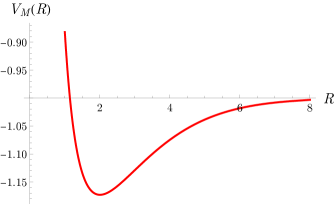
Figure 1: The nucleon potential $V_{M}(R)\equiv E_{e}(R)$ as the inter-nucleon distance, or bond length, $R$ is varied. The minimum is at $R_{0}=2.003$ in units of the reduced Bohr radius $\hat{a}_{0}$.

As explained above, in the Born-Oppenheimer approximation, the energy eigenvalue $E_{e}(R)$ is identified as the inter-nucleon potential $V_{M}(R)$. Its curvature at the minimum gives the fundamental vibrational frequency $\omega_{0}$ of the molecule. We find

$$\omega_{0}=\sqrt{\frac{1}{\mu}V_{M}^{{}^{\prime\prime}}(R_{0})}=0.020\,\hat{R}_{H}\ ,$$ (31)

that is, $\omega_{0}=0.275$ eV, or equivalently $2218\,\textrm{cm}^{-1}$.

The expectation values for the momentum, required to evaluate the potential $V_{\textrm{SME}}^{e}(R)$ are given by

$$\langle\,p^{a}\,p^{b}\,\rangle\,=\,-\int d^{3}\boldsymbol{r}\,\psi(\boldsymbol{r};R)\,\nabla^{a}\nabla^{b}\,\psi(\boldsymbol{r};R)\ ,$$ (32)

where we are working in the MOL frame where the $z$-axis is aligned with the molecular axis. Cylindrical symmetry then implies $\langle\,p^{x}p^{x}\,\rangle=\langle\,p^{y}p^{y}\,\rangle$, while $\langle p^{a}p^{b}\rangle$ vanishes for $a\neq b$. WIth $\gamma(R)$ set to 1, we find the analytic expressions

$$\langle\,p^{x}p^{x}\,\rangle_{1}\,=\,\langle p^{y}p^{y}\rangle_{1}\,=\,\frac{1}{3}\frac{1}{(1+I_{0})}\,\bigl{(}1+(1+R)e^{-R}\bigr{)}\ ,$$ (33)

and

$$\langle\,p^{z}p^{z}\,\rangle_{1}\,=\,\frac{1}{3}\frac{1}{(1+I_{0})}\,\bigl{(}1+(1+R-R^{2})e^{-R}\bigr{)}\ .$$ (34)

Reinstating $\gamma(R)$, in this case we have

$$\langle\,p^{a}p^{b}\,\rangle_{\gamma}(R)\,=\,\gamma(R)^{2}\,\langle\,p^{a}p^{b}\,\rangle_{1}(\gamma(R)R)\ .$$ (35)

These momentum expectation values are plotted in Fig. 2 (see also Fig. 5 in Appendix A. Since full spherical symmetry is restored as both $R\rightarrow 0$ and $R\rightarrow\infty$, we expect all three expectation values to be equal in these limits and related in the obvious way to the kinetic energy, implying (no sum on $a$) $\langle p^{a}\,p^{a}\rangle\rightarrow 4/3$ as $R\rightarrow 0$ and $\langle p^{a}\,p^{a}\rangle\rightarrow 1/3$ for large $R$. This is confirmed in the explicit numerical solutions.

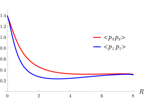
Figure 2: The momentum expectation values which determine the Lorentz and CPT violating contributions to the nucleon Schrödinger equation arising from the SME couplings of the electron as a function of the bond length $R$. The left hand figure shows $\langle p^{x}\,p^{x}\rangle$ (red,upper) and $\langle p^{z}\,p^{z}\rangle$ (blue) evaluated with the scaling factor $\gamma(R)$. The right hand figure is the same for ${\rm tr}\,\langle p^{a}\,p^{b}\rangle$ (red) and ${\rm tr}_{Y}\langle p^{a}\,p^{b}\rangle$ (blue) defined below.

Next, since these momentum expectation values are evaluated in the MOL frame whereas we want to express the rovibrational energies in terms of the Lorentz and CPT couplings $\tilde{E}_{ij}$ in the EXP frame, we need to find the relation between these frames.

The rotation matrix relating the EXP and MOL basis vectors, where $\boldsymbol{e}_{i}=\boldsymbol{e}_{a}\,R_{ai}$, is

$$R_{ai}\,=\,\begin{pmatrix}\cos\theta\,\cos\phi&~~~\cos\theta\,\sin\phi&~~~-\sin\theta\,\,\\ -\sin\phi&~~~\cos\phi&~~~0\\ \sin\theta\,\cos\phi&~~~\sin\theta\,\sin\phi&~~~\cos\theta\end{pmatrix}\ .$$ (36)

The angles $(\theta,\phi)$ here are the standard spherical polar coordinates specifying the orientation of the molecular axis in the EXP frame.

The SME couplings are then related by

$$\tilde{E}^{e}_{ab}\,=\,R_{ai}\,\tilde{E}^{e}_{ij}\,(R^{\textsf{T}})_{jb}\ .$$ (37)

The SME potential $V_{\textrm{SME}}^{e}(\boldsymbol{R})\,\equiv\,V_{\textrm{SME}}^{e}(R,\theta,\phi)$ in (17) is therefore

$$V_{\textrm{SME}}^{e}(R,\theta,\phi)\, =\,\frac{1}{m_{e}^{2}}\,\langle\,p^{a}\,p^{b}\,\rangle\,\tilde{E}^{e}_{ab}$$

$$=\,\frac{1}{m_{e}^{2}}\,\langle\,p^{a}\,p^{b}\,\rangle\,R_{ai}\,\tilde{E}^{e}_{ij}\,(R^{\textsf{T}})_{jb}$$ (38)

and using the cylindrical symmetry to set $\langle p^{y}p^{y}\rangle=\langle p^{x}p^{x}\rangle$, we can rewrite this as

$$V_{\textrm{SME}}^{e}(R,\theta,\phi)\,=\,\frac{1}{m_{e}^{2}}\,\Big{[}\,\langle\,p^{x}\,p^{x}\,\rangle\,\delta_{ij}~+~\bigl{(}\langle\,p^{z}\,p^{z}\,\rangle\,-\,\langle\,p^{x}\,p^{x}\,\rangle\bigr{)}\,(R^{\textsf{T}})_{iz}\,R_{zj}\,\Big{]}\,\tilde{E}^{e}_{ij}\ .$$ (39)

This greatly simplifies the calculation, since we now only need to evaluate the symmetric matrix

$$(R^{\textsf{T}})_{iz}\,R_{zj}\,=\,\begin{pmatrix}\sin^{2}\theta\,\cos^{2}\phi&~~~\tfrac{1}{2}\sin^{2}\theta\,\sin 2\phi&~~~\tfrac{1}{2}\sin 2\theta\,\cos\phi\,\,\\ \ldots&~~~\sin^{2}\theta\,\sin^{2}\phi&~~~\tfrac{1}{2}\sin 2\theta\,\sin\phi\\ \ldots&~~~\ldots&~~~\cos^{2}\theta\end{pmatrix}\ .$$ (40)

The final step to derive the potential $V_{\textrm{SME}}^{e}(R)$ to be used in the nucleon Schrödinger equation (18) is to take the expectation value in (19), viz.

$$V_{\textrm{SME}}^{e}(R)\,=\,\int d\Omega\,Y_{NM_{N}}^{*}(\theta,\phi)\,V_{\textrm{SME}}^{e}(R,\theta,\phi)\,Y_{NM_{N}}(\theta,\phi)\ .$$ (41)

Notice that this assumes the states are eigenstates of both $N$ and $M_{N}$. This will not necessarily be the case when we consider hyperfine-Zeeman splittings, and we return to this point in section 7. To evaluate (41), first expand $(R^{\textsf{T}})_{iz}\,R_{zj}$ in terms of spherical harmonics as

$$(R^{\textsf{T}})_{iz}\,R_{zj}\,=\,\sum_{M}\,C_{ij}^{M}\,Y_{2M}(\theta,\phi)\,+\,\tilde{C}_{ij}^{0}\,Y_{00}\ ,$$ (42)

with

$$C_{ij}^{M}\,=\,\int d\Omega\,(R^{\textsf{T}})_{iz}\,R_{zj}\,Y_{2M}(\theta,\phi)\ .$$ (43)

The combination $\tilde{C}_{ij}^{0}\,Y_{00}=1/3\,\delta_{ij}$ follows without further calculation by noting that ${\rm tr}\,(R^{\textsf{T}})_{iz}\,R_{zj}=1$ and ${\rm tr}\,C_{ij}^{M}=0$. In fact, we only need to calculate $C_{ij}^{M}$ for $M=0$, and with standard normalisations of the spherical harmonics we readily find Yoder:2012ks ,

$$C_{ij}^{0}\,=\,-\frac{2}{3}\sqrt{\frac{\pi}{5}}\,\begin{pmatrix}1~~~&0~~~&0\,\,\\ 0~~~&1~~~&0\\ 0~~~&0~~~&-2\end{pmatrix}\ .$$ (44)

The expectation value (41) is evaluated in terms of Clebsch-Gordan coefficients using the Gaunt integral,

$$\int d\Omega\,Y_{NM_{N}}^{*}(\theta,\phi)\,Y_{2M}(\theta,\phi)\,Y_{NM_{N}}(\theta,\phi)\,=\,\frac{1}{2}\sqrt{\frac{5}{\pi}}\,\,C_{NM_{N};20}^{NM_{N}}\,\,C_{N0;20}^{N0}\,\,\delta_{M0}\ ,$$ (45)

and we find

$$V_{\textrm{SME}}^{e}(R)\,=\,\, \frac{1}{m_{e}^{2}}\,\Big{[}\,\langle\,p^{x}\,p^{x}\,\rangle\,\delta_{ij}$$

$$+~\bigl{(}\langle\,p^{z}\,p^{z}\,\rangle\,-\,\langle\,p^{x}\,p^{x}\,\rangle\bigr{)}\,\,\Big{(}\frac{1}{2}\sqrt{\frac{5}{\pi}}\,C_{NM_{N};20}^{NM_{N}}\,C_{N0;20}^{N0}\,C_{ij}^{0}\,\,+\frac{1}{3}\,\delta_{ij}\Big{)}\Big{]}\,\tilde{E}^{e}_{ij}\ .$$ (46)

The Clebsch-Gordan coefficients are known analytically, and simplifying we have

$$C_{NM_{N};20}^{NM_{N}}\,C_{N0;20}^{N0}\,=\,\frac{N(N+1)-3M_{N}^{2}}{(2N-1)(2N+3)}\ ,$$ (47)

which vanishes for $N=0$. Collecting these results and rearranging, we therefore find our final result for the Lorentz and CPT violating contribution $V_{\textrm{SME}}^{e}(R)$ to the inter-nucleon potential Muller:2004tc ,

$$V_{\textrm{SME}}^{e}(R)\,=\,\,\frac{1}{3}\frac{1}{m_{e}^{2}}\,\Big{[} \,\big{(}2\langle\,p^{x}\,p^{x}\,\rangle\,+\langle\,p^{z}\,p^{z}\,\rangle\big{)}\,\,{\rm tr}\,\tilde{E}^{e}_{ij}$$

$$+~\bigl{(}\langle\,p^{z}\,p^{z}\,\rangle\,-\,\langle\,p^{x}\,p^{x}\,\rangle\bigr{)}\,\,\frac{N(N+1)-3M_{N}^{2}}{(2N-1)(2N+3)}\,\,\,{\rm tr}_{Y}\,\tilde{E}^{e}_{ij}\Big{]}\ ,$$ (48)

where we define ${\rm tr}_{Y}\,\tilde{E}_{ij}\,=\,\tilde{E}_{11}+\tilde{E}_{22}-2\tilde{E}_{33}$. As anticipated, the Lorentz and CPT violating couplings introduce an explicit $M_{N}$ dependence in $V_{\textrm{SME}}^{e}(R)$ ultimately breaking the degeneracy of the nucleon rovibrational levels with fixed $v,N$.

5 Rovibrational energy levels

We now move on to an explicit derivation of the rovibrational energy levels for the (anti-)hydrogen molecular ion, first without Lorentz and CPT violation and then incorporating the breaking potential $V_{\textrm{SME}}^{e}(R)$. We work analytically throughout, quoting our final answers in terms of derivatives of $V_{M}(R)$ and $V_{\textrm{SME}}^{e}(R)$ with respect to the inter-nucleon separation $R$, the latter being governed by the derivatives of the momentum expectation values in (46). Numerical estimates for these derivatives have been calculated in Appendix A, but we delay using these to keep maximum generality for as long as possible. An alternative approach, potentially more systematic, to calculating the rovibrational levels is given in Appendix B. Both approaches bring different physical insights into the physical origin of the various contributions to the energy levels.

We now pick up the discussion from the end of section 2. The first objective is to calculate the coefficients $x_{0},B_{0},\alpha_{0}$ and $D_{0}$ in the theory with no Lorentz or CPT violation. We start by including the angular momentum term in the nucleon Schrödinger equation (11) in an effective potential $V_{\it eff}(R)$ and study the simple harmonic motion about the minimum of this potential. So we define

$$V_{\it eff}(R)\,=\,V_{M}(R)\,+\,\frac{1}{2\mu R^{2}}\,N(N+1)\ .$$ (49)

The angular momentum term changes the mean inter-nucleon separation (bond length) and the vibration frequency perturbatively in the small parameter $\lambda=1/(\mu\,\omega_{0}R_{0}^{2})$ that was introduced in section 2.

First, let $R_{m}=R_{0}+\delta R$ be the minimum of the effective potential. Setting $V_{\it eff}^{{}^{\prime}}(R_{m})=0$, we find

$$\frac{\delta R}{R_{0}}\,=\,\lambda^{2}\,N(N+1)\,-\,\Big{(}3\,+\,\frac{1}{2}\frac{R_{0}V_{M}^{{}^{\prime\prime\prime}}(R_{0})}{V_{M}^{{}^{\prime\prime}}(R_{0})}\Big{)}\,\lambda^{4}\,(N(N+1))^{2}\,+\,\ldots$$ (50)

The corresponding shift in the bond length is interpreted as “centrifugal stretching” as the centrifugal force due to the orbital angular momentum stretches the effective spring binding the nucleons.

Evaluating the effective potential at the new minimum gives

$$V_{\it eff}(R_{m})\, =\,V_{\it eff}(R_{0})\,+\,\delta R\,V_{\it eff}^{\prime}(R_{0})\,+\,\frac{1}{2}\delta R^{2}\,V_{\it eff}^{{}^{\prime\prime}}(R_{0})\,+\,\ldots$$

$$=V_{M}(R_{0})\,+\,\frac{1}{2}\lambda\,N(N+1)\,\omega_{0}\,-\,\frac{1}{2}\lambda^{3}\,(N(N+1))^{2}\,\omega_{0}\,+\,\ldots$$ (51)

The coefficient of this $O(N(N+1))^{2}$ term is of importance later. It arises here as a combination of two terms, one with a pre-factor $-1$ from the $O(\delta R)$ contribution, where it is interpreted as reduced kinetic energy due to centrifugal stretching at fixed $N$, and one with pre-factor 1/2 from the $O(\delta R)^{2}$ contribution which is interpreted as the extra potential energy due to this stretching of the inter-nucleon bond.

Next, we need the change in the effective vibrational frequency due to expanding about the minimum of $V_{\it eff}(R)$. Here,

$$V_{\it eff}^{{}^{\prime\prime}}(R_{m})\, =\,V_{\it eff}^{{}^{\prime\prime}}(R_{0})\,+\,\delta R\,V_{\it eff}^{{}^{\prime\prime\prime}}(R_{0})\,+\,\ldots$$

$$=\,V_{M}^{{}^{\prime\prime}}(R_{0})\,\Big{[}\,1\,+\,\Big{(}3\,+\,\frac{R_{0}V_{M}^{{}^{\prime\prime\prime}}(R_{0})}{V_{M}^{{}^{\prime\prime}}(R_{0})}\,\Big{)}\,\lambda^{2}\,N(N+1)\,+\,O(\lambda^{4}\ (N(N+1))^{2})\,\Big{]}\ .$$ (52)

We have also calculated the $O(\lambda^{4}\,(N(N+1))^{2})$ term here, which has a coefficient involving up to four derivatives of the potential $V_{M}(R)$. These lead to contributions to the rovibrational energy (12) of $O\big{(}(v+\tfrac{1}{2})(N(N+1))^{2}\big{)}$, which are obviously very small and are omitted in this paper for simplicity.

The new oscillation frequency $\omega$ is then

$$\omega\,=\,\omega_{0}\,\Big{[}1\,+\,\frac{1}{2}\Big{(}3\,+\,\frac{R_{0}V_{M}^{{}^{\prime\prime\prime}}(R_{0})}{V_{M}^{{}^{\prime\prime}}(R_{0})}\Big{)}\,\lambda^{2}\,N(N+1)\,+\,\ldots\,\Big{]}\ ,$$ (53)

with a corresponding contribution $(v+\tfrac{1}{2})\,\omega$ to the energy.

The term proportional to $V_{M}^{{}^{\prime\prime\prime}}(R_{0})$ in (53), which contributes to the coefficient $\alpha_{0}$ below, has an interesting interpretation in terms of “vibrational stretching” of the bond length in the presence of an asymmetric potential. In particular, in the case of an anharmonic oscillator with a cubic interaction, the expectation value of the position is shifted from the minimum of the potential. Applying this result to the expansion of the angular momentum term $V_{N}(R)$ in (49),

$$V_{N}(R)\,=\,\frac{1}{2}\lambda\,\omega_{0}\,N(N+1)\,\Big{(}1\,-\,2\,\frac{\langle\,x\,\rangle}{R_{0}}\,+\,\ldots\Big{)}\ ,$$ (54)

where we write $R=R_{0}+x$, and evaluating $\langle x\rangle$ approximating $V_{M}(R)$ as an anharmonic oscillator, we have

$$\frac{\langle\,x\,\rangle}{R_{0}}\,=\,-\frac{1}{2}\,\lambda\,\frac{R_{0}V_{M}^{{}^{\prime\prime\prime}}(R_{0})}{V_{M}^{{}^{\prime\prime}}(R_{0})}\,(v+\tfrac{1}{2})\ ,$$ (55)

which reproduces the equivalent term in the energy found through the alternative route in (53). This derivation makes clear that this is an increase in kinetic energy at fixed $N$ due to the reduction in mean bond length from (55).

Finally, collecting all these results, we find the coefficients in the expansion

$$E_{vN}\,=\, (v+\tfrac{1}{2})\,\omega_{0}\,-\,x_{0}\,(v+\tfrac{1}{2})^{2}\,\omega_{0}$$

$$+\,B_{0}\,N(N+1)\,\omega_{0}\,-\,\alpha_{0}\,(v+\tfrac{1}{2})N(N+1)\,\omega_{0}\,-\,D_{0}\,(N(N+1))^{2}\,\omega_{0}\,+\,\ldots$$ (56)

of the rovibrational energies are

$$B_{0}\, =\,\frac{1}{2}\,\lambda~\ ,~~~~ \alpha_{0}\, =\,-\frac{1}{2}\Big{(}3\,+\,\frac{R_{0}V_{M}^{{}^{\prime\prime\prime}}}{V_{M}^{{}^{\prime\prime}}}\,\Big{)}\,\lambda^{2}~\ ,$$

$$D_{0}\, =\,\frac{1}{2}\,\lambda^{3}~\ , x_{0}\, =\,\left[\frac{5}{48}\,\Big{(}\frac{R_{0}V_{M}^{{}^{\prime\prime\prime}}}{V_{M}^{{}^{\prime\prime}}}\Big{)}^{2}\,-\,\frac{1}{16}\,\Big{(}\frac{R_{0}^{2}V_{M}^{(4)}}{V_{M}^{{}^{\prime\prime}}}\Big{)}\,\right]\,\lambda~\ ,$$ (57)

where all the indicated derivatives of $V_{M}(R)$ are taken at $R_{0}$.

The result for $x_{0}$ arises from taking into account the anharmonic nature of the potential and including the $O(v+\tfrac{1}{2})^{2}$ contributions to the energy of an anharmonic oscillator with a $gx^{3}\,+\,hx^{4}$ potential, where we identify $g=\tfrac{1}{6}V_{M}^{{}^{\prime\prime\prime}}$ and $h=\tfrac{1}{24}V_{M}^{(4)}$. These are proportional to $h$ at first order and $g^{2}$ at second order. The explicit formulae, which determine $x_{0}$ in (57), are quoted in footnote 12.

Importantly, each quoted coefficient is the leading term in an expansion in $\lambda$. At each order, the prefactors are known numbers involving successively higher derivatives of the basic inter-nucleon potential. We have derived these in Appendix A to a precision sufficient for our purpose here, which is to determine the leading corrections to (56) when Lorentz and CPT violating interactions are introduced.

We now need to extend this calculation to include the Lorentz and CPT violating potential $V_{\textrm{SME}}^{e}(R)$ in the nucleon Schrödinger equation. The idea is to iterate the effective potential method for the hierarchy of perturbations, first including only the angular momentum term as above, then including the potential $V_{\textrm{SME}}^{e}(R)$ as a further small perturbation. As always, the Lorentz and CPT perturbations are considered the smallest, and we work only to first order in the SME couplings so terms of $O(V_{\textrm{SME}}^{e})^{2}$ are immediately dropped.

So here we define

$$U_{\it eff}(R)\,=\,V_{\it eff}(R)\,+\,V_{\textrm{SME}}^{e}(R)\ ,$$ (58)

and expand about the minimum $R_{u}$ of $U_{\it eff}(R)$. Setting $U_{\it eff}^{\prime}(R_{u})=0$ with $R_{u}=R_{m}+\delta R_{u}$, we have

$$\frac{\delta R_{u}}{R_{m}}\,=\,-\frac{1}{R_{m}V_{\it eff}^{{}^{\prime\prime}}(R_{m})}\,V_{\textrm{SME}}^{e\,^{\prime}}(R_{m})\ .$$ (59)

We then find, repeating the steps (51) and (52) above and neglecting terms of $O(\textrm{SME})^{2}$, that

$$U_{\it eff}(R_{u})\, =\,U_{\it eff}(R_{m})\,+\,\delta R_{u}\,U_{\it eff}^{\prime}(R_{m})$$

$$=\,V_{\it eff}(R_{m})\,+\,V_{\textrm{SME}}^{e}(R_{m})\ ,$$ (60)

and

$$U_{\it eff}^{{}^{\prime\prime}}(R_{u})\,=\,V_{\it eff}^{{}^{\prime\prime}}(R_{m})\,+\,V_{\textrm{SME}}^{e\,^{\prime\prime}}(R_{m})\,-\,\frac{V_{\it eff}^{{}^{\prime\prime\prime}}(R_{m})}{V_{\it eff}^{{}^{\prime\prime}}(R_{m})}\,V_{\textrm{SME}}^{e\,^{\prime}}(R_{m})\ ,$$ (61)

the latter giving the new effective vibration frequency $\omega_{u}$.

The next step is to rewrite (60) and (61) in terms of derivatives at the minimum $R_{0}$ of the original potential $V_{M}(R)$, rather than at $R_{m}$. We have already found $V_{\it eff}(R_{m})$ and $V_{\it eff}^{{}^{\prime\prime}}(R_{m})$ in (51) and (52), so we just need

$$U_{\it eff}(R_{u})\, =\,V_{\it eff}(R_{m})\,+\,V_{\textrm{SME}}^{e}(R_{0})\,+\,\delta R\,V_{\textrm{SME}}^{e\,^{\prime}}(R_{0})\,+\,\frac{1}{2}\delta R^{2}\,V_{\textrm{SME}}^{e\,^{\prime\prime}}(R_{0})$$

$$=\,V_{\it eff}(R_{m})\,+\,V_{\textrm{SME}}^{e}(R_{0})$$

$$~~~~+\,\Big{[}\lambda^{2}\,N(N+1)-\Big{(}3\,+\,\frac{1}{2}\frac{R_{0}V_{M}^{{}^{\prime\prime\prime}}}{V_{M}^{{}^{\prime\prime}}}\,\Big{)}\,\lambda^{4}\,(N(N+1))^{2}\Big{]}\,R_{0}\,V_{\textrm{SME}}^{e\,^{\prime}}(R_{0})$$

$$~~~~+\,\frac{1}{2}\lambda^{4}\,(N(N+1))^{2}\,R_{0}^{2}\,V_{\textrm{SME}}^{e\,^{\prime\prime}}(R_{0})\ ,$$ (62)

which gives the Lorentz and CPT violating contributions $B_{\rm SME}^{e}$ and $D_{\rm SME}^{e}$ in (65) below, then from (61), and after some lengthy but straightforward algebra, we find

$$U_{\it eff}^{{}^{\prime\prime}}(R_{u})\, =\,V_{\it eff}^{{}^{\prime\prime}}(R_{m})\,+\,V_{\textrm{SME}}^{e\,^{\prime\prime}}(R_{0})\,-\,\frac{V_{M}^{{}^{\prime\prime\prime}}}{V_{M}^{{}^{\prime\prime}}}\,V_{\textrm{SME}}^{e\,^{\prime}}(R_{0})$$

$$~~~+\,\lambda^{2}\,N(N+1)\Big{[}R_{0}\,V_{\textrm{SME}}^{e\,^{\prime\prime\prime}}(R_{0})\,-\,\frac{V_{M}^{{}^{\prime\prime\prime}}}{V_{M}^{{}^{\prime\prime}}}\Big{(}R_{0}\,V_{\textrm{SME}}^{e\,^{\prime\prime}}(R_{0})\,+\,\beta\,V_{\textrm{SME}}^{e\,^{\prime}}(R_{0})\Big{)}\,\Big{]}\ ,$$ (63)

again with the understanding that all derivatives of $V_{M}$ are taken at $R_{0}$. Here,

$$\beta\,=\,3\,-\,12\,\frac{V_{M}^{{}^{\prime\prime}}}{R_{0}\,V_{M}^{{}^{\prime\prime\prime}}}\,-\,\frac{R_{0}\,V_{M}^{{}^{\prime\prime\prime}}}{V_{M}^{{}^{\prime\prime}}}\,+\,\frac{R_{0}\,V_{M}^{(4)}}{V_{M}^{{}^{\prime\prime\prime}}}\ .$$ (64)

The new effective vibration frequency is now given by $\omega_{u}^{2}=\omega_{0}^{2}\,U_{\it eff}^{{}^{\prime\prime}}(R_{0})/V_{M}^{{}^{\prime\prime}}(R_{0})$ and the corresponding energy levels by $(v+\tfrac{1}{2})\,\omega_{u}$. This gives contributions to $\alpha_{\rm SME}^{e}$ and $\delta_{\rm SME}^{e}$, defined below.

The Lorentz and CPT corrections to the rovibrational energies (56) can therefore be written in the form

$$E_{vNM_{N}}\,=\, (1+\delta_{\rm SME}^{e})\,(v+\tfrac{1}{2})\,\omega_{0}\,-\,(x_{0}+x_{\rm SME}^{e})\,(v+\tfrac{1}{2})^{2}\,\omega_{0}$$

$$+\,(B_{0}+B_{\rm SME}^{e})\,N(N+1)\,\omega_{0}\,-\,(\alpha_{0}+\alpha_{\rm SME}^{e})\,(v+\tfrac{1}{2})N(N+1)\,\omega_{0}$$

$$-\,(D_{0}+D_{\rm SME}^{e})\,(N(N+1))^{2}\,\omega_{0}\,+\,\ldots$$ (65)

with coefficients

$$\delta_{\rm SME}^{e}\, =\,\frac{1}{2}\,\frac{1}{V_{M}^{{}^{\prime\prime}}}\,\Big{[}\,V_{\rm SME}^{e\,^{\prime\prime}}\,-\,\frac{V_{M}^{{}^{\prime\prime\prime}}}{V_{M}^{{}^{\prime\prime}}}\,\,V_{\rm SME}^{e\,^{\prime}}\Big{]}$$

$$B_{\rm SME}^{e}\, =\,\lambda\,\,\frac{1}{V_{M}^{{}^{\prime\prime}}}\,\Big{[}\frac{1}{R_{0}}\,V_{\rm SME}^{e\,^{\prime}}\,\Big{]}$$

$$\alpha_{\rm SME}^{e}\, =\,\lambda^{2}\,\,\frac{1}{V_{M}^{{}^{\prime\prime}}}\,\bigg{[}-\frac{1}{2}R_{0}\,V_{\rm SME}^{e\,^{\prime\prime\prime}}\,+\,\frac{3}{4}\Big{(}1+\frac{R_{0}\,V_{M}^{{}^{\prime\prime\prime}}}{V_{M}^{{}^{\prime\prime}}}\Big{)}\,V_{\rm SME}^{e\,^{\prime\prime}}$$

$$~~~~~~~~~~~~~~~~~~~~~~~~~~~~-\,\Big{(}6\,+\,\frac{9}{4}\,\frac{R_{0}\,V_{M}^{{}^{\prime\prime\prime}}}{V_{M}^{{}^{\prime\prime}}}\,+\,\frac{3}{4}\Big{(}\frac{R_{0}\,V_{M}^{{}^{\prime\prime\prime}}}{V_{M}^{{}^{\prime\prime}}}\Big{)}^{2}\,-\,\frac{1}{2}\frac{R_{0}^{2}\,V_{M}^{(4)}}{V_{M}^{{}^{\prime\prime}}}\Big{)}\,\frac{1}{R_{0}}\,V_{\rm SME}^{e\,^{\prime}}\bigg{]}$$

$$D_{\rm SME}^{e}\, =\,\lambda^{3}\,\,\frac{1}{V_{M}^{{}^{\prime\prime}}}\,\Big{[}-\frac{1}{2}\,V_{\rm SME}^{e\,^{\prime\prime}}\,+\,\Big{(}3\,+\,\frac{1}{2}\frac{R_{0}\,V_{M}^{{}^{\prime\prime\prime}}}{V_{M}^{{}^{\prime\prime}}}\,\Big{)}\,\frac{1}{R_{0}}\,V_{\rm SME}^{e\,^{\prime}}\,\Big{]}\ .$$ (66)

The final coefficient $x_{\rm SME}^{e}$ is found from the anharmonic terms as before, where here $g=\tfrac{1}{6}U_{\it eff}^{{}^{\prime\prime\prime}}(R_{u})$ and $h=\tfrac{1}{24}U_{\it eff}^{(4)}(R_{u})$. Since we are not calculating terms involving the angular momentum at $O(v+\tfrac{1}{2})^{2}$, we may simplify $U_{\it eff}(R)$ in (58) to be just $V_{M}(R)+V_{\rm SME}^{e}(R)$, with the corresponding simplification of $\delta R_{u}$ in (59). Then we use the AHO energies in footnote 12 to extract $x_{\rm SME}^{e}$, keeping terms of first order in the SME couplings only. There are two sources of extra terms beyond the simple extension of $x_{0}$ in (57). The first comes from writing the derivatives at $R_{0}$ rather than $R_{u}$; thus, for example, $U_{\it eff}^{(4)}(R_{u})\rightarrow V_{M}^{(4)}(R_{0})\,+\,V_{\rm SME}^{e\,(4)}(R_{0})\textsection\,+\,\delta R_{u}\,V_{M}^{(5)}(R_{0})$, which produces extra terms proportional to $V_{\rm SME}^{e\,^{\prime}}$. Next, we must remember that the frequency in the AHO energies is now $\omega_{u}$ not $\omega_{0}$, where $\mu\,\omega_{u}^{2}=U_{\it eff}^{{}^{\prime\prime}}(R_{u})$ in (63). Including both corrections eventually gives

$$x_{\rm SME}^{e}\, =\,\lambda\,\,\frac{1}{V_{M}^{{}^{\prime\prime}}}\,\bigg{[}\frac{5}{24}\,R_{0}^{2}\,\frac{V_{M}^{{}^{\prime\prime\prime}}}{V_{M}^{{}^{\prime\prime}}}\,\bigg{(}\,V_{\rm SME}^{e\,^{\prime\prime\prime}}\,-\,\frac{V_{M}^{{}^{\prime\prime\prime}}}{V_{M}^{{}^{\prime\prime}}}\,V_{\rm SME}^{e\,^{\prime\prime}}\,+\,\Big{(}\,\Big{(}\frac{V_{M}^{{}^{\prime\prime\prime}}}{V_{M}^{{}^{\prime\prime}}}\Big{)}^{2}\,-\,\frac{V_{M}^{(4)}}{V_{M}^{{}^{\prime\prime}}}\,\Big{)}V_{\rm SME}^{e\,^{\prime}}\bigg{)}~~~~~~~~~~~~~~$$

$$~~~~~~~~~~-\,\frac{1}{16}\,R_{0}^{2}\,\bigg{(}\,V_{\rm SME}^{e\,(4)}\,-\,\frac{V_{M}^{(4)}}{V_{M}^{{}^{\prime\prime}}}\,V_{\rm SME}^{e\,^{\prime\prime}}\,+\,\Big{(}\,\frac{V_{M}^{{}^{\prime\prime\prime}}V_{M}^{(4)}}{(V_{M}^{{}^{\prime\prime}})^{2}}\,-\,\frac{V_{M}^{(5)}}{V_{M}^{{}^{\prime\prime}}}\,\Big{)}\,V_{\rm SME}^{e\,^{\prime}}\,\bigg{)}\bigg{]}\ .$$ (67)

We should perhaps emphasise that while these expressions appear complicated, the coefficients of $V_{\rm SME}^{e}$ and its derivatives are just simple numerical factors determined by $V_{M}(R)$ and have been evaluated in Appendix A. That said, all the $V_{M}$-dependent terms shown in these coefficients are necessary, since there is no reason to discard those with higher derivatives of $V_{M}$ as being smaller. As a check that the effective potential method used here has indeed correctly and completely identified all the terms occurring at the required order in $\lambda$, we present an alternative, especially systematic, perturbative method of evaluation in Appendix B.

At this point, in addition to the rovibrational energies themselves, we can deduce expressions for the Lorentz and CPT violating effects on the mean inter-nucleon bond length and the dissociation energy.

As well as the $N$-dependent centrifugal stretching, the mean bond length is also affected by the SME couplings. This contribution, $\Delta R_{SME}$, is simply identified in the effective potential method as $\delta R_{u}$ in (59). Expanding the potentials $V_{\rm SME}^{e\,^{\prime}}(R_{m})$ and $V_{\it eff}^{{}^{\prime\prime}}(R_{m})$ about $R_{0}$ instead of $R_{m}$, we find

$$\Delta R_{\rm SME}\,=\,-\frac{1}{V_{M}^{{}^{\prime\prime}}}\,\Big{[}V_{\rm SME}^{e\,^{\prime}}\,+\,\lambda^{2}\,N(N+1)\,\Big{(}R_{0}\,V_{\rm SME}^{e\,^{\prime\prime}}\,-\,\Big{(}3\,+\,\frac{R_{0}V_{M}^{{}^{\prime\prime\prime}}}{V_{M}^{{}^{\prime\prime}}}\Big{)}\,V_{\rm SME}^{e\,^{\prime}}\,\Big{)}\,\Big{]}\ ,$$ (68)

up to higher order terms of $O\big{(}\lambda^{2}\,N(N+1)\big{)}^{2}$.

We define the dissociation energy $E^{\it diss}$ as the difference between the energy of the ground state and the value of the inter-nucleon potential in the large-$R$ limit. The SME correction to the dissociation energy is then,

$$\Delta\,E_{\rm SME}^{\it diss}\,=\,V_{\rm SME}^{e}(\infty)\,-\,V_{\rm SME}^{e}(R_{0})\,-\,\frac{1}{2}\,\delta_{\rm SME}^{e}\,\omega_{0}\ .$$ (69)

This is evaluated explicitly in the following section, noting that since $\langle p^{a}\,p^{b}\rangle\,\rightarrow\,(1/3)\delta^{ab}$ as $R\rightarrow\infty$, reflecting the spherical symmetry in this limit, the second term in (48) for $V_{\rm SME}^{e}(\infty)$ vanishes.

The remaining contribution to the rovibrational energies comes from the direct contribution $\Delta E_{\rm SME}^{n}$ from the Lorentz and CPT violating proton couplings $E_{ij}^{p}$ in the nucleon Schrödinger equation. Recall from (20) that this requires us to evaluate the expectation value

$$\Delta E_{\textrm{SME}}^{n}\,=\,\frac{2}{m_{p}^{2}}E_{ij}^{p}\,\langle v\,NM_{N}|\,P^{i}P^{j}\,|v\,NM_{N}\rangle\ ,$$ (70)

in the original nucleon states $|v\,NM_{N}\rangle$, with all quantities expressed in the EXP frame. The analysis mirrors that described in detail in section 4. First, we expand $P^{i}P^{j}$ in spherical harmonics,

$$P_{i}\,P_{j}\,=\,P^{2}\,\Big{(}\frac{1}{3}\,\delta_{ij}\,+\,\sum_{M}C_{ij}^{M}\,Y_{2M}(\theta,\phi)\,\Big{)}\ ,$$ (71)

where $(\theta,\phi)$ are the spherical polar angles made by the molecular axis (and therefore $\boldsymbol{P}$) in the EXP frame, i.e. $P_{i}=|\boldsymbol{P}|(\sin\theta\cos\phi,\sin\theta\sin\phi,\cos\theta)$. Noting then that $P_{i}P_{j}=P^{2}\,(R^{T})_{iz}R_{zj}$, which of course is inherent in the construction of (40), the coefficient $C_{ij}^{M}$ here is identical to that found in section 4. Taking the expectation value as in (45) and evaluating the Clebsch-Gordan equations (47), we find without further calculation that

$$\Delta E_{SME}^{n}\,=\,\langle vN|\,P^{2}\,|vN\rangle\,\frac{2}{m_{p}^{2}}\,\Big{[}\,\frac{1}{3}\,{\rm tr}\,E_{ij}^{p}\,-\,\frac{1}{3}\,\,\frac{N(N+1)-3M_{N}^{2}}{(2N-1)(2N+3)}\,\,{\rm tr}_{Y}\,E_{ij}^{p}\,\Big{]}$$ (72)

The problem therefore reduces to finding the expectation value $\langle\,P^{2}\,\rangle$ of the nucleon momentum. In this case, we do not have a simple explicit wave function solving the Schrödinger equation, so a direct evaluation is not straightforward. However, since $P^{2}/2\mu$ is just the kinetic energy, all we need in practice is to identify the kinetic energy part of the total rovibrational energy $E_{vN}$ in (56). This requires examining each of the coefficients $x_{0},B_{0},\alpha_{0}$ and $D_{0}$ derived above and deducing on physical grounds what is their kinetic energy component.

First, write (72) as

$$\Delta E_{\rm SME}^{n}\,=\,\langle v\,N|\,K\,|v\,N\rangle\,\tilde{V}_{\rm SME}^{n}\ ,$$ (73)

with

$$\tilde{V}_{\rm SME}^{n}\,=\,\frac{2}{3}\frac{1}{m_{p}}\Big{[}\,{\rm tr}\,E_{ij}^{p}\,-\,\,\frac{N(N+1)-3M_{N}^{2}}{(2N-1)(2N+3)}\,\,{\rm tr}_{Y}\,E_{ij}^{p}\,\Big{]}\ .$$ (74)

Then, adding this contribution to (65), the rovibrational energies including all the Lorentz and CPT breaking contributions are written as

$$E_{vNM_{N}}\,=\, (1+\delta_{\rm SME}^{e}+\delta_{\rm SME}^{n})\,(v+\tfrac{1}{2})\,\omega_{0}\,-\,(x_{0}+x_{\rm SME}^{e}+x_{\rm SME}^{n})\,(v+\tfrac{1}{2})^{2}\,\omega_{0}$$

$$+\,(B_{0}+B_{\rm SME}^{e}+B_{\rm SME}^{n})\,N(N+1)\,\omega_{0}\,$$

$$-\,(\alpha_{0}+\alpha_{\rm SME}^{e}+\alpha_{\rm SME}^{n})\,(v+\tfrac{1}{2})N(N+1)\,\omega_{0}$$

$$-\,(D_{0}+D_{\rm SME}^{e}+D_{\rm SME}^{n})\,(N(N+1))^{2}\,\omega_{0}\,+\,\ldots$$ (75)

Beginning with the angular momentum independent terms, $x_{0}$ is found to $O(\lambda)$ by approximating $V_{M}(R)$ as an anharmonic oscillator with cubic and quartic interactions. An explicit calculation, consistent with the virial theorem, shows that at $O(v+1/2)$ the kinetic energy is $E_{v}/2$ while at $O(v+1/2)^{2}$ the whole energy is kinetic. It follows immediately that the corresponding coefficients in (75) are

$$\delta_{\rm SME}^{n}\,=\,\frac{1}{2}\,\tilde{V}_{\rm SME}^{n}\ ,~~~~~~~~~~~~~~~~x_{\rm SME}^{n}\,=\,x_{0}\,\tilde{V}_{\rm SME}^{n}\ .~~~~~~~~~~~$$ (76)

Turning to the $N$-dependent terms, it is clear that $B_{0}$ is a pure kinetic energy term. However, For $D_{0}$ we emphasised above there were two contributions, weighted -1 and 1/2, which arose due to centrifugal stretching. Of these the first represents a reduction in kinetic energy, while the second is potential energy due to stretching the mean bond length. This means we must take

$$B_{\rm SME}^{n}\,=\,B_{0}\,\tilde{V}_{\rm SME}^{n}\ ,~~~~~~~~~~~~~~D_{\rm SME}^{n}\,=\,2\,D_{0}\,\tilde{V}_{\rm SME}^{n}\ .~~~~~~~$$ (77)

For $\alpha_{0}$, we invoke the interpretation in terms of vibrational stretching to argue that the $O(V_{M}^{{}^{\prime\prime\prime}}$ contribution reflects the reduction in mean bond length as a result of the anharmonic terms in the potential, and that both terms arise from the purely kinetic term $N(N+1)/2\mu R^{2}$ in the Schrödinger equation. We therefore take

$$\alpha_{\rm SME}^{n}\,=\,\alpha_{0}\,\tilde{V}_{\rm SME}^{n}\ .~~~~~~~~~~~~~~~~~~~~~~~~~~~~~~~~~~~~~~~~~~~~~~~~$$ (78)

Together, (74) to (78) complete the derivation of the Lorentz and CPT violating contributions to the rovibrational energy levels.

6 The rovibrational spectrum

In this section, we draw together all the results of sections 4 and 5 and the appendices to describe the implications of Lorentz and CPT violation for the rovibrational spectrum of the (anti-)hydrogen molecular ion.

First, we verify that our approximate methods describe the rovibrational spectrum in the absence of Lorentz and CPT symmetry breaking sufficiently for our objective, that is to constrain the SME couplings with greater precision than is possible with atomic (anti-)hydrogen alone. For this, we need the numerical results for $V_{M}(R)$ and its derivatives tabulated in Appendix A, Table 1. The key result is for the vibrational frequency $\omega_{0}$. Converting from the atomic units of Table 1 using $\hat{R}_{H}=1/(2\hat{\mu}\,\hat{a}_{0}^{2})$, we find

$$\omega_{0}\,=\,\sqrt{\frac{2V_{M}^{{}^{\prime\prime}}(R_{0})}{m_{p}}}~=~0.020\,\hat{R}_{H}~=~0.275\,{\rm eV}~=~2218\,{\rm cm}^{-1}\ ,$$ (79)

where in standard spectroscopic units (with $h=c=1$), $1\,{\rm eV}\,=\,2.418\times 10^{14}\,{\rm Hz}\,=\,8065.5\,{\rm cm}^{-1}$.

The dimensionless expansion parameter $\lambda$ is then determined for the $H_{2}^{+}$ ion as $\lambda\,=\,1/(\mu\omega_{0}R_{0}^{2})\,=\,0.027$.

The coefficients of the expansion (56) of the rovibrational energy levels,

$$E_{vN}\,=\, (v+\tfrac{1}{2})\,\omega_{0}\,-\,x_{0}\,(v+\tfrac{1}{2})^{2}\,\omega_{0}$$

$$+\,B_{0}\,N(N+1)\,\omega_{0}\,-\,\alpha_{0}\,(v+\tfrac{1}{2})N(N+1)\,\omega_{0}\,-\,D_{0}\,(N(N+1))^{2}\,\omega_{0}\,+\,\ldots$$ (80)

are then found from Table 1 to be

$$B_{0}\, =\,\frac{1}{2}\,\lambda\,=\,0.0135\ ,~~~~~~~~~~~~~~~~~~\alpha_{0}\,=\,1.133\,\lambda^{2}\,=\,0.819\times 10^{-3}\ ,$$

$$D_{0}\, =\,\frac{1}{2}\,\lambda^{3}\,=\,1.944\times 10^{-5}~~~~~~~~~~~~x_{0}\,=\,1.230\,\lambda\,=\,0.033\,\ .$$ (81)

Substituting back, we find the rovibrational levels in spectroscopic units of $\rm{cm}^{-1}$ in the form,

$$E_{vN}\,=\, 2218\,(v+\tfrac{1}{2})\,-\,73.2\,(v+\tfrac{1}{2})^{2}\,$$

$$+\,29.82\,N(N+1)\,-\,1.82\,(v+\tfrac{1}{2})N(N+1)\,-\,0.0216\,(N(N+1))^{2}\,+\,\ldots$$ (82)

which may be compared with precision calculations and data. The hierarchy of the coefficients in powers of $\lambda$ is immediately evident. A particular point of interest already here is that the term in (57) involving the third derivative $V_{M}^{{}^{\prime\prime\prime}}$ is essential even to give the correct sign for the $O(v+\tfrac{1}{2})\,N(N+1)$ contribution. Moreover, the $x_{0}$ coefficient, which is determined entirely by the higher derivative terms in $V_{M}(R)$, has the correct value and sign to produce the narrowing of vibrational energy level splittings as $v$ becomes larger, allowing roughly 20 vibrational states below the dissociation energy. Both these observations confirm the necessity of including a full analysis of the anharmonic terms in $V_{M}(R)$ to produce a realistic match to the rovibrational spectrum and ensure our results remain valid beyond the lowest vibrational states.

We now turn to the Lorentz and CPT violating effects in the rovibrational spectrum. Writing the coefficients $\delta_{\rm SME}^{e}$, $B_{\rm SME}^{e},\ldots$ in (66), (67) in terms of $V_{\rm SME}^{e}$ and its derivatives using the numerical values in Table 1 gives, in atomic units,

$$\delta_{\rm SME}^{e}\, =\,\,\big{[}\,2.669\,V_{\rm SME}^{e\,^{\prime\prime}}\,+\,7.018\,V_{\rm SME}^{e\,^{\prime}}\,\big{]}$$

$$B_{\rm SME}^{e}\, =\,\,\,\lambda\,\big{[}\,2.664\,V_{\rm SME}^{e\,^{\prime}}\,\big{]}$$

$$\alpha_{\rm SME}^{e}\, =\,\lambda^{2}\,\big{[}-5.346\,V_{\rm SME}^{e\,^{\prime\prime\prime}}\,-\,17.084\,V_{\rm SME}^{e\,^{\prime\prime}}\,-\,3.408\,V_{\rm SME}^{e\,^{\prime}}\,\big{]}$$

$$D_{\rm SME}^{e}\, =\,\lambda^{3}\,\big{[}\,-2.669\,V_{\rm SME}^{e\,^{\prime\prime}}\,+\,0.897\,V_{\rm SME}^{e\,^{\prime}}\,\big{]}$$

$$x_{\rm SME}^{e}\, =\,\,\,\lambda\,\big{[}\,-1.337\,V_{\rm SME}^{e\,(4)}\,-\,11.738\,V_{\rm SME}^{e\,^{\prime\prime\prime}}\,-\,22.004\,V_{\rm SME}^{e\,^{\prime\prime}}\,-\,5.215\,V_{\rm SME}^{e\,^{\prime}}\,\big{]}\ .$$ (83)

The next step is to re-express $V_{\rm SME}^{e}$ in (48) in atomic units, as assumed here. Recalling $R_{H}\,=\,1/(2\,m_{e}\,a_{0}^{2})$, we write $V_{\rm SME}^{e}(R)$ as

$$V_{\rm SME}^{e}(R)\,=\,\Big{[}\,\frac{2}{3}\,{\rm tr}\,\langle p^{a}\,p^{b}\rangle\,\,\frac{1}{m_{e}}\,{\rm tr}\,\tilde{E}_{ij}^{e}~-~\frac{1}{3}\,{\rm tr}_{Y}\langle p^{a}\,p^{b}\rangle\,\,c_{NM_{N}}\,\frac{1}{m_{e}}\,{\rm tr}_{Y}\tilde{E}_{ij}^{e}\,\Big{]}\ ,$$ (84)

where we now introduce the shorthand,

$$c_{NM_{N}}\,=\,\frac{N(N+1)-3M_{N}^{2}}{(2N-1)(2N+3)}\ ,$$ (85)

and the momentum expectation values and their derivatives take their numerical values as given in Table 1. Substituting these values, we can express the coefficients in (83) directly in terms of the SME couplings ${\rm tr}\,\tilde{E}_{ij}^{e}$ and ${\rm tr}_{Y}\tilde{E}_{ij}^{e}$ as follows:

$$\delta_{\rm SME}^{e}\, =\,\,\big{[}-1.000\,\frac{1}{m_{e}}\,{\rm tr}\,\tilde{E}_{ij}^{e}\,+\,0.272\,c_{NM_{N}}\,\frac{1}{m_{e}}\,{\rm tr}_{Y}\tilde{E}_{ij}^{e}\,\big{]}$$

$$B_{\rm SME}^{e}\, =\,\,\,\lambda\,\big{[}-0.666\,\frac{1}{m_{e}}\,{\rm tr}\,\tilde{E}_{ij}^{e}\,+\,0.112\,c_{NM_{N}}\,\frac{1}{m_{e}}\,{\rm tr}_{Y}\tilde{E}_{ij}^{e}\,\big{]}$$

$$\alpha_{\rm SME}^{e}\, =\,\lambda^{2}\,\big{[}-2.152\,\frac{1}{m_{e}}\,{\rm tr}\,\tilde{E}_{ij}^{e}\,+\,0.095\,c_{NM_{N}}\,\frac{1}{m_{e}}\,{\rm tr}_{Y}\tilde{E}_{ij}^{e}\,\big{]}$$

$$D_{\rm SME}^{e}\, =\,\lambda^{3}\,\big{[}-0.979\,\frac{1}{m_{e}}\,{\rm tr}\,\tilde{E}_{ij}^{e}\,+\,0.060\,c_{NM_{N}}\,\frac{1}{m_{e}}\,{\rm tr}_{Y}\tilde{E}_{ij}^{e}\,\big{]}$$

$$x_{\rm SME}^{e}\, =\,\,\,\lambda\,\big{[}-1.629\,\frac{1}{m_{e}}\,{\rm tr}\,\tilde{E}_{ij}^{e}\,+\,0.065\,\,c_{NM_{N}}\,\frac{1}{m_{e}}\,{\rm tr}_{Y}\tilde{E}_{ij}^{e}\,\big{]}\ .$$ (86)

For reference, we also quote here the equivalent results for the coefficients $\delta_{\rm SME}^{n},\,B_{\rm SME}^{n},\ldots$ in the same format. From (74), (76)-(78) and (81) we find:

$$\delta_{\rm SME}^{n}\, =\,\,\,0.333\,\big{[}\,\frac{1}{m_{p}}\,{\rm tr}\,{E}_{ij}^{p}\,-\,c_{NM_{N}}\,\frac{1}{m_{p}}\,{\rm tr}_{Y}{E}_{ij}^{p}\,\big{]}$$

$$B_{\rm SME}^{n}\, =\,\,0.333\,\lambda\,\big{[}\,\frac{1}{m_{p}}\,{\rm tr}\,{E}_{ij}^{p}\,-\,c_{NM_{N}}\,\frac{1}{m_{p}}\,{\rm tr}_{Y}{E}_{ij}^{p}\,\big{]}$$

$$\alpha_{\rm SME}^{n}\, =\,0.755\,\lambda^{2}\,\big{[}\,\frac{1}{m_{p}}\,{\rm tr}\,{E}_{ij}^{p}\,-\,c_{NM_{N}}\,\frac{1}{m_{p}}\,{\rm tr}_{Y}{E}_{ij}^{p}\,\big{]}$$

$$D_{\rm SME}^{n}\, =\,0.667\,\lambda^{3}\,\big{[}\,\frac{1}{m_{p}}\,{\rm tr}\,{E}_{ij}^{p}\,-\,c_{NM_{N}}\,\frac{1}{m_{p}}\,{\rm tr}_{Y}{E}_{ij}^{p}\,\big{]}$$

$$x_{\rm SME}^{n}\, =\,\,0.820\,\lambda\,\big{[}\,\frac{1}{m_{p}}\,{\rm tr}\,{E}_{ij}^{p}\,-\,\,c_{NM_{N}}\,\frac{1}{m_{p}}\,{\rm tr}_{Y}{E}_{ij}^{p}\,\big{]}\ .$$ (87)

We can also write the expressions for the SME corrections to the mean bond length and dissociation energy in this form. From the leading term in (68), omitting the weak $N$-dependence of $O\big{(}\lambda^{2}\,N(N+1)\big{)}$ here, we find

$$\Delta R_{\rm SME}\,=\,\big{[}\,1.340\,\frac{1}{m_{e}}\,{\rm tr}\,\tilde{E}_{ij}^{e}\,-\,0.226\,c_{NM_{N}}\,\frac{1}{m_{e}}\,{\rm tr}_{Y}\tilde{E}_{ij}^{e}\,\big{]}\ .$$ (88)

The dissociation energy is defined in (69) in terms of $V_{\rm SME}^{e}(R_{0})$, given in (84), $V_{\rm SME}^{e}(\infty)$, where ${\rm tr}\,\langle p^{a}\,p^{b}\rangle\,\rightarrow\,1$ and ${\rm tr}_{Y}\langle\ p^{a}\,p^{b}\rangle\,\rightarrow\,0$, and $\delta_{\rm SME}^{e}$, which modifies the ground state energy. Substituting from Table 1, we then find

$$\Delta E_{\rm SME}^{\it diss}\,=\,\big{[}-0.105\,\frac{1}{m_{e}}\,{\rm tr}\,\tilde{E}_{ij}^{e}\,+\,0.117\,\,c_{NM_{N}}\,\frac{1}{m_{e}}\,{\rm tr}_{Y}\tilde{E}_{ij}^{e}\,\big{]}\ ,$$ (89)

where both $\Delta R_{\rm SME}$ and $\Delta E_{\rm SME}^{\it diss}$ in (88) and (89) are in atomic units.

Finally, to make contact with previous work, we should express ${\rm tr}\,\tilde{E}_{ij}^{e},\,{\rm tr}_{Y}\tilde{E}_{ij}^{e}$ and ${\rm tr}\,{E}_{ij}^{p},\,{\rm tr}_{Y}{E}_{ij}^{p}$ directly in terms of the original SME couplings in the Lagrangian (1).

It is often convenient in spectroscopy applications to use a spherical harmonic decomposition of the SME couplings. To make the translation, we need to compare the non-relativistic Hamiltonian $H_{\rm SME}^{\rm NR}$ in (13) with its equivalent in terms of the SME couplings $c_{njm}^{\rm NR}$ and $a_{njm}^{\rm NR}$ in the spherical harmonic basis,

$$H_{\rm SME}^{\rm NR}\,=\,-\sum_{njm}\,\big{(}c_{njm}^{\rm NR}\,-\,a_{njm}^{\rm NR}\big{)}\,|\boldsymbol{p}|^{n}\,Y_{jm}(\hat{\boldsymbol{p}})\,+\,\ldots$$ (90)

where $\ldots$ represents the spin-dependent couplings in $B_{k}$, $D_{k}$ and $F_{ijk}$. Specialising to the terms with $n=2$, we then write

$$p^{i}\,p^{j}\,=\,\Big{(}\frac{1}{3}\delta_{ij}\,+\,\sum_{m}\,C_{ij}^{m}\,Y_{2m}(\hat{\boldsymbol{p}})\,\Big{)}\,|\boldsymbol{p}|^{2}\ ,$$ (91)

and comparing coefficients of the spherical harmonics between (13) and (90), using (44) for $C_{ij}^{0}$, we identify

$$\frac{1}{m}\,{\rm tr}\,{E}_{ij}\,=\,-3m\,\frac{1}{\sqrt{4\pi}}\,\big{(}c_{200}^{\rm NR}\,-\,a_{200}^{\rm NR}\big{)}\ ,~~~~~~~~~~~~\frac{1}{m}\,{\rm tr}_{Y}{E}_{ij}\,=\,3m\,\sqrt{\frac{5}{4\pi}}\,\big{(}c_{220}^{\rm NR}\,-\,a_{220}^{\rm NR}\big{)}\ .~~~~\\$$ (92)

with the obvious extension to $\tilde{E}_{ij}^{e}=E_{ij}^{e}\,+\,\frac{1}{2}(m_{e}^{2}/m_{p}^{2})E_{ij}^{p}$,  and $E_{ij}^{p}$. In terms of the original SME couplings in (14), we therefore have

$$\frac{1}{\sqrt{4\pi}}\,c_{200}^{\rm NR}\, =\,\,\frac{1}{3m}\big{(}c_{ii}\,+\,\tfrac{3}{2}c_{00}\big{)}\ ,~~~~~~~~~~~\frac{1}{\sqrt{4\pi}}\,a_{200}^{\rm NR}\,=\,\,a_{0ii}\,+\,a_{000}\ ,$$

$$\sqrt{\frac{5}{4\pi}}\,c_{220}^{\rm NR}\, =\,-\frac{1}{3m}\,{\rm tr}_{Y}c_{ij}\ ,~~~~~~~~~~~~~~~~~\sqrt{\frac{5}{4\pi}}\,a_{220}^{\rm NR}\,=\,-{\rm tr}_{Y}a_{0ij}\ .$$ (93)

Altogether, equations (75) with (81), (86), (87) and (92) complete our description of the dependence of the rovibrational energy levels $E_{vNM_{N}}$ of the molecular (anti-)hydrogen ion on the spin-independent SME couplings.

7 Rovibrational transitions

In this final section, we take a first look at how the results in section 6 may be used to constrain the Lorentz and CPT couplings through measurements of the rovibrational transitions ${\rm H}_{2}^{+}$, and eventually its antimatter counterpart $\overline{\rm H}_{2}^{\,-}$, and explain why these offer the possibility of improving existing bounds on the spin-independent SME couplings by several orders of magnitude. Further discussion, together with an assessment of current and future experimental possibilities, will be presented elsewhere.

We begin by describing some basic features of the spectrum of the molecular hydrogen ion (see, for example, SchillerCP ). Since the $1s\,\sigma_{g}$ electron state in ${\rm H}_{2}^{+}$ is symmetric, the total nucleon state must be antisymmetric under exchange of the two protons – this implies that for even $N$, the two protons are in an antisymmetric spin state $I=0$ (where $\boldsymbol{I}$ is the sum of the spins of the two protons), while for odd $N$, the spin state is symmetric so $I=1$. These two groupings are referred to as Para- and Ortho-${\rm H}_{2}^{+}$ respectively. Since ${\rm H}_{2}^{+}$ is a homonuclear molecule, it has no permanent dipole moment and electric dipole transitions (denoted E1) between rovibrational states (which would allow $\Delta N=1$ transitions) are forbidden. The remaining possibilities are single-photon electric quadrupole (E2) and two-photon (TP) transitions, for which the selection rule $\Delta N\,=\,0,\,\pm 2$ applies (with $N=0\rightarrow N=0$ transitions disallowed for E2 but permitted for TP only). These selection rules therefore forbid transitions between the Ortho and Para states, so their spectra are essentially independent of each other.

To illustrate some of the possibilities of constraining the SME couplings by precision measurements of rovibrational transitions, we consider here just the leading coefficients $\delta_{\rm SME}^{e,\,p}$ and $B_{\rm SME}^{e,\,p}$ from (87). In this case,

$$E_{vNM_{N}}\,=\,(v+\tfrac{1}{2})\,\omega_{0}\,\Big{[}\,1\,+\,\frac{\,\,\,1}{\sqrt{4\pi}}\Big{(}3.00\,m_{e}\big{(}\tilde{c}_{200}^{{\rm NR}\,e}\,-\,\tilde{a}_{200}^{{\rm NR}\,e}\big{)}\,-\,m_{p}\big{(}c_{200}^{{\rm NR}\,p}\,-\,a_{200}^{{\rm NR}\,p}\big{)}\Big{)}$$

$$~~~~~~~~~~~~~~~~~~~~~~~~~~~+\,\sqrt{\frac{5}{4\pi}}\,c_{NM_{N}}\,\Big{(}0.82\,m_{e}\big{(}\tilde{c}_{220}^{{\rm NR}\,e}\,-\,\tilde{a}_{220}^{{\rm NR}\,e}\big{)}\,-\,m_{p}\big{(}c_{220}^{{\rm NR}\,p}-a_{220}^{{\rm NR}\,p}\big{)}\,\Big{)}\,\Big{]}$$

$$~~~+\,\frac{1}{2}\lambda\,N(N+1)\,\omega_{0}\,\Big{[}\,1\,+\,\frac{\,\,\,1}{\sqrt{4\pi}}\Big{(}3.99\,m_{e}\big{(}\tilde{c}_{200}^{{\rm NR}\,e}\,-\,\tilde{a}_{200}^{{\rm NR}\,e}\big{)}\,-\,2\,m_{p}\big{(}c_{200}^{{\rm NR}\,p}\,-\,a_{200}^{{\rm NR}\,p}\big{)}\Big{)}$$

$$~~~~~~~~~~~~~~~~~~~~~~~~~+\,\sqrt{\frac{5}{4\pi}}\,c_{NM_{N}}\,\Big{(}0.67\,m_{e}\big{(}\tilde{c}_{220}^{{\rm NR}\,e}\,-\,\tilde{a}_{220}^{{\rm NR}\,e}\big{)}\,-\,2\,m_{p}\big{(}c_{220}^{{\rm NR}\,p}-a_{220}^{{\rm NR}\,p}\big{)}\,\Big{)}\,\Big{]}\ ,$$ (94)

with $\tilde{c}_{200}^{{\rm NR}\,e}=c_{200}^{{\rm NR}\,e}+\tfrac{1}{2}\,c_{200}^{{\rm NR}\,p}$, etc.

The simplest case is a transition where the angular momentum quantum number is unchanged, i.e. $\Delta v\neq 0$ but $\Delta N=0$ (and $\Delta M_{N}=0$). In this case,

$$\frac{\Delta E_{\rm SME}}{\Delta E}\, =\,\delta_{\rm SME}^{e}\,+\,\delta_{\rm SME}^{p}$$

$$=\,\frac{\,\,\,1}{\sqrt{4\pi}}\,\Big{[}\,3.00\,m_{e}\big{(}\tilde{c}_{200}^{{\rm NR}\,e}\,-\,\tilde{a}_{200}^{{\rm NR}\,e}\big{)}\,-\,1.00\,m_{p}\big{(}c_{200}^{{\rm NR}\,p}\,-\,a_{200}^{{\rm NR}\,p}\big{)}$$

$$~~+\,\frac{N(N+1)-3M_{N}^{2}}{(2N-1)(2N+3)}\,\sqrt{5}\,\,\Big{(}0.82\,m_{e}\big{(}\tilde{c}_{220}^{{\rm NR}\,e}\,-\,\tilde{a}_{220}^{{\rm NR}\,e}\big{)}\,-\,m_{p}\big{(}c_{220}^{{\rm NR}\,p}-a_{220}^{{\rm NR}\,p}\big{)}\,\Big{)}\,\Big{]}\ .$$ (95)

This already demonstrates a number of important features. First, even for a purely vibrational transition, the Clebsch-Gordan factor $c_{NM_{N}}$ arising with the $(njm)\,=\,(200)$ SME couplings implies that the transition frequency is dependent on $N$ and $M_{N}$. By comparing transitions with different $N$, it is then possible to separate the contributions from the $(200)$ and $(220)$ couplings, which can therefore be constrained individually.

Conversely, it is evident from (94) that even a purely rotational transition Alighanbari:2020 with $\Delta N\neq 0$ but $\Delta v=0$ will also depend on the vibrational quantum number $v$ through the (220) couplings.

Furthermore, because of the different numerical coefficients of the electron and proton terms in $\delta_{\rm SME}$ and $B_{\rm SME}$, by comparing different transitions where $\Delta v\neq 0,\,\Delta N=0$, or $\Delta v=0,\,\Delta N\neq 0$, or both non-zero, it is also possible to distinguish the contributions from $\big{(}\tilde{c}_{200}^{{\rm NR}\,e}\,-\,\tilde{a}_{200}^{{\rm NR}\,e}\big{)}$ and the purely proton coupling $\big{(}c_{200}^{{\rm NR}\,p}\,-\,a_{200}^{{\rm NR}\,p}\big{)}$. Similarly for the $(220)$ couplings. A relatively small number of rovibrational transitions in ${\rm H}_{2}^{+}$ could therefore lead to precision constraints on all four types of $(c_{njm}^{\rm NR}\,-\,a_{njm}^{\rm NR})$ couplings in (94).

Finally, if similar precision experiments become possible with the antihydrogen molecular ion Myers ; Karr:2018 ; Zammit , then because the $c_{njm}^{\rm NR}$ couplings are CPT even while the $a_{njm}^{\rm NR}$ couplings are CPT-odd, taking the difference of the ${\rm H}_{2}^{+}$ and $\overline{\rm H}_{2}^{\,-}$ spectra would isolate the dependence on the $a_{njm}^{\rm NR}$ couplings. This would allow individual constraints to be placed on all 8 SME couplings in (94).

To see why these constraints are potentially so powerful for the molecular ions, we should compare with the equivalent transitions with atomic hydrogen and antihydrogen. Keeping only the spin-independent SME couplings, we find for the $1{S}_{d}$ - $2{S}_{d}$ transition Kostelecky:2015nma ; Charlton:2020kie measured for antihydrogen by ALPHA Ahmadi:2018eca (where the suffix $d$ labels the particular hyperfine state),

$$\frac{\Delta E^{\rm SME}_{1S_{d}\,-\,2S_{d}}}{\Delta E_{1S\,-\,2S}}\,=\,\frac{2m_{e}}{\sqrt{4\pi}}\Big{[}\big{(}c_{200}^{{\rm NR}\,e}\,-\,a_{200}^{{\rm NR}\,e}\big{)}\,+\,\big{(}c_{200}^{{\rm NR}\,p}\,-\,a_{200}^{{\rm NR}\,p}\big{)}\,\Big{]}\ .$$ (96)

Notice this is only sensitive to the $(njm)=(200)$ couplings.

To access a transition sensitive to the $(njm)=(220)$ couplings in (anti-)hydrogen, we need to consider a state with electron orbital momentum $\ell\neq 0$ (in the same way that we require $N\neq 0$ to access the $(220)$ contributions to the rovibrational states in (94)). ALPHA has measured the $1S_{d}$ - $2P_{c-}$ transition ALPHA:2020rbx for which we can show Kostelecky:2015nma ; Charlton:2020kie ,

$$\frac{\Delta E^{\rm SME}_{1S_{d}\,-\,2P_{c-}}}{\Delta E_{1S\,-\,2S}}\, =\,\frac{2m_{e}}{\sqrt{4\pi}}\,\Big{[}\big{(}c_{200}^{{\rm NR}\,e}\,-\,a_{200}^{{\rm NR}\,e}\big{)}\,+\,\big{(}c_{200}^{{\rm NR}\,p}\,-\,a_{200}^{{\rm NR}\,p}\big{)}$$

$$~~~~~~~~~\,-\,\frac{\sqrt{5}}{\,\,30}\,(1\,+\,3\cos{2\eta})\,\Big{(}\,\big{(}{c}_{220}^{{\rm NR}\,e}\,-\,{a}_{220}^{{\rm NR}\,e}\big{)}\,+\,\big{(}c_{220}^{{\rm NR}\,p}-a_{220}^{{\rm NR}\,p}\big{)}\,\Big{)}\,\Big{]}\ ,$$ (97)

where $\cos\eta$ is a magnetic field dependent mixing angle.

This brings us to the key point. Focusing on the CPT violating couplings, the two-photon $1S$ -$2S$ transition in (anti-)hydrogen constrains the combination

$$m_{e}\,\big{(}a_{200}^{{\rm NR}\,e}\,+\,a_{200}^{{\rm NR}\,p}\big{)}\,\lesssim\,R_{1S-2S}\ ,$$ (98)

where $R_{1S-2S}$ is the relative precision of the measurement. ALPHA has measured this transition for antihydrogen with a precision $R_{1S-2S}\simeq 2\times 10^{-12}$ Ahmadi:2018eca , while a precision of $O(10^{-15})$ is known for hydrogen Parthey:2011lfa ; Matveev:2013orb . Knowing this, the single-photon $1S$ -$2P$ transition, which is measured by ALPHA with the much weaker precision $R_{1S-2P}\simeq 10^{-8}$ ALPHA:2020rbx , constrains the $(220)$ combination,

$$m_{e}\,\big{(}a_{220}^{{\rm NR}\,e}\,+\,a_{220}^{{\rm NR}\,p}\big{)}\,\lesssim\,R_{1S-2P}\ .$$ (99)

With just four measurements, $1S$ - $2S$ and $1S$ - $2P$ for hydrogen and antihydrogen, we are able to constrain only the combinations (98), (99) of electron and proton couplings, and similar for the $c_{njm}^{\rm NR}$. Crucially, both the electron and proton couplings are multiplied by $m_{e}$.

In contrast, for ${\rm H}_{2}^{+}$, by measuring only a small number of rovibrational transitions as indicated above, together with the equivalent for $\overline{\rm H}_{2}^{\,-}$, we have sufficient data to constrain all 8 coefficients. Denoting the precisions generically by $R_{rovib}$, in this case we find the constraints,

$$m_{e}\,\big{(}a_{200}^{{\rm NR}\,e}\,+\,\tfrac{1}{2}a_{200}^{{\rm NR}\,p}\big{)}\,\lesssim\,R_{rovib}\ ,~~~~~~~~~~~~~m_{p}\,a_{200}^{{\rm NR}\,p}\,\lesssim\,R_{rovib}\ ,$$ (100)

and

$$m_{e}\,\big{(}a_{220}^{{\rm NR}\,e}\,+\,\tfrac{1}{2}a_{200}^{{\rm NR}\,p}\big{)}\lesssim\,R_{rovib}\ ,~~~~~~~~~~~~~~m_{p}\,a_{220}^{{\rm NR}\,p}\,\lesssim\,R_{rovib}\ ,$$ (101)

with equivalent bounds for the $c_{njm}^{\rm NR}$. Here, we have written out in full the couplings $\tilde{c}_{njm}^{\rm NR\,e}$ and $\tilde{a}_{njm}^{\rm NR\,e}$. Notice that the bounds on the proton SME couplings arising from their indirect influence on the electron Schrödinger equation have the same $m_{e}$ mass dependence as those found in the atomic transitions. This is not true of the proton couplings arising directly in the nucleon Schrödinger equation, which involve $m_{p}$ itself.

So not only do the rovibrational transitions allow us to constrain the electron and proton couplings separately, the constraint on the proton couplings $a_{200}^{{\rm NR}\,p}$ and $a_{220}^{{\rm NR}\,p}$ is enhanced by a factor $m_{p}/m_{e}\sim 10^{3}$ compared to the atomic transitions. This is in addition to the potential enhancement from the greater precision of frequency measurements for the rovibrational transitions, which of course is especially marked for the $(220)$ couplings where the precision of the $1S$ - $2P$ measurement in antihydrogen is necessarily 4 orders of magnitude below that achieved for $1S$ - $2S$.

So far, we have only considered the rovibrational states to be described by quantum numbers $v,N,M_{N}$ and have neglected spin (see Korobov2006 ; KKH20081 ; KKH20082 ). In general, the $1s\sigma_{g}$ states in ${\rm H}_{2}^{+}$ will be labelled as $|v\,N\,I\,S\,F\,J\,M_{J}\rangle$, according to the angular momentum addition scheme $\boldsymbol{F}=\boldsymbol{I}+\boldsymbol{S}$, where $\boldsymbol{I}$ and $\boldsymbol{S}$ are the total nucleon and electron spins respectively, followed by $\boldsymbol{J}=\boldsymbol{N}+\boldsymbol{F}$.

The hyperfine structure is then determined by a Hamiltonian incorporating 5 combinations of spin-spin and spin-orbit interactions, with known coefficients calculated at $O(\alpha^{2})$ to six-figure precision in QED Korobov2006 . This simplifies greatly for the case of Para-$\textrm{H}_{2}^{\,+}$ and we illustrate our results for this case here. The energy eigenstates, at zero background magnetic field, are then $|v\,N\,S\,J\,M_{J}\rangle$ with $S=1/2$ always and $\boldsymbol{J}=\boldsymbol{N}+\boldsymbol{S}$. The corresponding hyperfine interaction is simply,

$$H_{\rm HFS}\,=\,c_{e}(v,N)\,\boldsymbol{N}.\boldsymbol{S}~~=~\frac{1}{2}c_{e}(v,N)\,\big{(}\boldsymbol{J}^{2}-\boldsymbol{N}^{2}-\boldsymbol{S}^{2}\big{)}\ .$$ (102)

The values of $c_{e}(v,N)$ for low values of $v$ and $N$ are given in Table 1 of Korobov2006 . It follows directly that the rovibrational energies are split by the value of $J=N\pm 1/2$ as follows,

$$\Delta E_{\rm HFS}\, =\,\,\frac{1}{2}\,c_{e}(v,N)\,N\ ,~~~~~(J=N+\tfrac{1}{2})$$

$$=\,-\frac{1}{2}\,c_{e}(v,N)\,(N+1)\ ,~~~~~(J=N-\tfrac{1}{2})\ ,$$ (103)

and are degenerate with respect to $M_{J}$. As we now show, this $M_{J}$ degeneracy is broken by the spin-independent SME couplings.

To calculate the SME contributions to the hyperfine states, we first express the eigenstates $|J\,M_{J}\rangle$ in terms of the $|M_{N}\,M_{S}\rangle$ basis states through Clebsch-Gordan coefficients as follows,

$$|J\,M_{J}\rangle\,\,=\,\,\sum_{M_{S}}\,C^{J\,M_{J}}_{N\,M_{N},\,\tfrac{1}{2}\,M_{S}}\,\,|M_{N}\,M_{S}\rangle\ ,~~~~~~~(M_{N}=M_{J}-M_{S})\ .$$ (104)

Now, at the point (41) for the electron $V^{e}_{\rm SME}(R)$, or (72) for the proton $\tilde{V}^{n}_{\rm SME}$, our derivation of the rovibrational energies requires the evaluation of $\sum_{M}\,C_{ij}^{M}\,Y_{2M}$ between eigenstates, taken there to be $|v\,N\,M_{N}\rangle$. Using the hyperfine states $|J\,M_{J}\rangle$ instead, we find

$$E_{ij}\,\sum_{M}\,C_{ij}^{M}\,\langle J\,M_{J}|Y_{2M}\,|J\,M_{J}\rangle$$

$$~~~~~~~~~~~=\,E_{ij}\,\,\sum_{M_{S}}\,C_{ij}^{0}\,\big{(}C^{J\,M_{J}}_{N\,M_{N},\,\tfrac{1}{2}\,M_{S}}\big{)}^{2}\,\langle M_{N}\,M_{S}|\,Y_{20}\,|M_{N}\,M_{S}\rangle~~~~~~~$$

$$~~~~~~~~~~~\,=\,-\frac{1}{3}\,{\rm tr}_{Y}E_{ij}\,\,\sum_{M_{S}}\,\big{(}C^{J\,M_{J}}_{N\,M_{N},\,\tfrac{1}{2}\,M_{S}}\big{)}^{2}\,\,c_{N(M_{J}-M_{S})}\ ,$$ (105)

in terms of the factor $c_{NM_{N}}$ in (85). In the first step, spin-independence requires the matrix element to be diagonal in $M_{S}$ and hence also in $M_{N}=M_{J}-M_{S}$. This restricts as before to $M=0$ in the spherical harmonic expansion. (This is no longer true for the spin-dependent couplings, which acquire an extra, off-diagonal contribution at this point, involving the coefficients $C_{ij}^{\pm 1}$.) In the second step, we have substituted (44) for the coefficient $C_{ij}^{0}$, giving the usual combination ${\rm tr}_{Y}E_{ij}$ of the SME couplings.

The Clebsch-Gordan factors may be evaluated algebraically for $J=N\pm 1/2$ separately, and in both cases we find,

$$E_{ij}\,\sum_{M}\,C_{ij}^{M}\,\langle J\,M_{J}|Y_{2M}\,|J\,M_{J}\rangle~=~-\frac{1}{3}\,{\rm tr}_{Y}E_{ij}\,\,\frac{1}{4J(J+1)}\,\big{(}J(J+1)\,-\,3M_{J}^{2}\big{)}\ .$$ (106)

The only change needed to convert the rovibrational energies calculated above to the hyperfine states $|J\,M_{J}\rangle$ is therefore the replacement of $c_{NM_{N}}$ by $c_{JM_{J}}$ where

$$c_{JM_{J}}\,=\,\frac{\big{(}J(J+1)\,-\,3M_{J}^{2}\big{)}}{4J(J+1)}\ .$$ (107)

This confirms how the spin-independent SME couplings break the degeneracy with respect to $M_{J}$ of the hyperfine energy levels.

In practice, spectroscopy will be performed in a background magnetic field, which we may use to define the $3$-axis of the EXP frame, $\boldsymbol{B}=(0,0,B)$. The rovibrational energies will therefore acquire a shift due to the Zeeman effect. Restricting again to Para-$\textrm{H}_{2}^{\,+}$, the Zeeman Hamiltonian is

$$H_{Z}\,=\,g_{e}\mu_{B}\,\boldsymbol{S}.\boldsymbol{B}\,-\,\mu_{p}\,\boldsymbol{N}.\boldsymbol{B}\ ,$$ (108)

where $\mu_{p}=e/2m_{p}$ is much smaller than the Bohr magneton, so the electron spin dominates the energy shifts. For large $B$, where the hyperfine splitting is negligible compared to the Zeeman effect, the combined hyperfine-Zeeman eigenstates become approximately just the $|v\,N\,S\,M_{N}\,M_{S}\rangle$ states. For intermediate magnetic fields, apart from the extremal states $|J=N+\tfrac{1}{2},M_{J}=\pm(N+\tfrac{1}{2})\rangle\,\equiv\,|M_{N}=\pm N,\,M_{S}=\pm\tfrac{1}{2}\rangle$ where the two bases coincide, the remaining $4N$ hyperfine-Zeeman eigenstates are mixed pairwise, with $2N$ $B$-dependent mixing angles.

Our original derivation of the rovibrational energy levels therefore applies directly in the large $B$ regime where the eigenstates are essentially given by $|M_{N}\,M_{S}\rangle$, and the results above with $c_{NM_{N}}$ hold, showing the extra $M_{N}$ dependence of the energy levels due to the SME couplings. For intermediate values of the magnetic field, the corresponding SME energies involving $c_{220}^{\rm NR}$ and $a_{220}^{NR}$ will depend in an individually state-specific way on the mixing angles.

Our focus in this paper has been on the spin-independent SME couplings, for reasons given above. Inclusion of the spin-dependent couplings is in principle a straightforward extension of the results given here, though inevitably more complicated in general given the spin dependence of the hyperfine states. Here, we just outline some key features of the calculation.

Including the pure spin terms $B_{k}^{e}\,S_{k}$ and $B_{k}^{p}\,I_{k}$ for the electron and proton is simple, requiring only the Clebsch-Gordan coefficients to evaluate the expectation values of the spins in the hyperfine states. The couplings $F^{e}_{ijk}\,S_{k}$ and $F^{p}_{ijk}\,I_{k}$ require more analysis. Again restricting to the much simpler case of Para-${\rm H}_{2}^{\,+}$ where we need only consider the electron spin, we find the spin-dependent contribution to $V^{e}_{\rm SME}(R)$ in (39), (41) in the hyperfine states in the form,

$$V^{e,\,spin}_{\rm SME}(R)\, =\,\frac{1}{m_{e}^{2}}\Big{[}\,\frac{1}{3}\,{\rm tr}\,\langle p^{a}\,p^{b}\rangle\,\langle J\,M_{J}|\,S_{k}\,|J\,M_{J}\rangle\,\delta_{ij}\,F^{e}_{ijk}$$

$$~~~~~~~~~~-\frac{1}{2}\,{\rm tr}_{Y}\langle p^{a}\,p^{b}\rangle\,\sum_{M}\,\langle J\,M_{J}|\,C_{ij}^{M}\,Y_{2M}\,S_{k}\,|J\,M_{J}\rangle\,F^{e}_{ijk}\,\Big{]}\ .$$ (109)

Evaluation of the second term is similar to (105) except that, apart from the extremal states, the hyperfine eigenstates $|J\,M_{J}\rangle$ are linear combinations of spin eigenstates so as well as contributions from $S_{3}$ we have additional contributions from the raising and lowering operators $S_{\pm}=S_{1}\pm iS_{2}$. Such terms are familiar from analysis of transitions involving $2P$ states in (anti-)hydrogen Charlton:2020kie . Since these states also mix different values of $M_{N}$ along with different $M_{S}$, the matrix elements now receive contributions from the spherical harmonics $Y_{2M}$ with $M=\pm 1$ as well as $M=0$ as before. These involve the coefficients $C_{ij}^{\pm 1}$ where Yoder:2012ks ,

$$C_{ij}^{\pm 1}\,=\,\sqrt{\frac{2\pi}{15}}\,\begin{pmatrix}0~~~&0~~~&\mp 1\,\,\\ 0~~~&0~~~&i\\ \mp 1~~~&i~~~&0\end{pmatrix}\ .$$ (110)

We therefore find three distinct contributions to $V^{e,\,spin}_{\rm SME}(R)$ from the $F^{e}_{ijk}$ couplings, taking the forms

$${\rm tr}\,\langle p^{a}\,p^{b}\rangle\,\,{\rm tr}\,F_{ij3}\,M_{J}\ ,~~~~~~{\rm tr}_{Y}\langle p^{a}\,p^{b}\rangle\,\,{\rm tr}_{Y}F_{ij3}\,M_{J}\ ,~~~~~~{\rm tr}_{Y}\langle p^{a}\,p^{b}\rangle\,\,(F_{+3-}\,+\,F_{-3+})\,M_{J}\ ,$$

where the traces on $F_{ij3}^{e}$ are on the $(i,j)$ indices. Each of these spin-dependent contributions is found to be proportional to $M_{J}$, together with Clebsch-Gordan pre-factors depending algebraically on the quantum numbers $N,J$ and $M_{J}$. These expressions then carry through exactly as in the text to give contributions analogous to (86) to the rovibrational energies in the hyperfine states.

Finally, apart from precision measurements of rovibrational energy levels, including a comparison of ${\rm H}_{2}^{\,+}$ and $\overline{\rm H}_{2}^{\,-}$ as a direct CPT test, Lorentz symmetry breaking would reveal itself through annual (and sidereal) variations in the transition frequencies resulting from the SME coupling contributions derived above. This analysis is well-known (see e.g. Kostelecky:2008ts ) and we only comment briefly here.

The first step is to rewrite the SME couplings in components referred to the standard SUN frame (see section 3). In general this involves a rotation from the EXP to SUN frames, which depends on the location and orientation of the background magnetic field of the particular experiment. Note, however, that this rotation does not affect the isotropic $(200)$ couplings, which retain their form in the SUN frame.

These SUN frame couplings are then subject to a Lorentz transformation with velocity $v_{\oplus}$ of $O(10^{-4})$ corresponding to the Earth’s rotation around the Sun, resulting in small periodic variations with the Earth’s orbit. In SUN frame coordinates $(T,X,Y,Z)$, the orbital velocity is

$$\boldsymbol{v}_{\oplus}\,=\,v_{\oplus}\,\Big{(}\sin\Omega_{\oplus}T\,\boldsymbol{e}_{X}-\cos\Omega_{\oplus}T\big{(}\cos\eta\,\boldsymbol{e}_{Y}\,+\,\sin\eta\,\boldsymbol{e}_{Z}\big{)}\Big{)}\ ,$$ (111)

where $\Omega_{\oplus}$ is the orbital frequency and $\eta=23.4^{\circ}$ is the tilt angle between the Earth’s equator and the orbital plane. The isotropic SME couplings in the rovibrational energy levels are simply $\tfrac{1}{\sqrt{4\pi}}\,c_{200}^{\rm NR}\,=\,\tfrac{1}{3m}\big{(}\tfrac{3}{2}c_{TT}+c_{KK}\big{)}$ and $\tfrac{1}{\sqrt{4\pi}}\,a_{200}^{\rm NR}\,=\,a_{TTT}+a_{TKK}$. Applying a Lorentz transformation with $\boldsymbol{v}_{\oplus}$ then gives the periodic variation of the combinations of isotropic SME couplings appearing in the rovibrational energies (94) as,

$$\tfrac{1}{\sqrt{4\pi}}\,\delta_{\oplus}\big{(}c_{200}^{\rm NR}-a_{200}^{\rm NR}\big{)}\, =\,v_{\oplus}\sin\Omega_{\oplus}T\Big{(}\tfrac{5}{3m}c_{XT}-5a_{XTT}-a_{XKK}\Big{)}$$

$$~~~-v_{\oplus}\cos\Omega_{\oplus}T\Big{(}\cos\eta\,\big{(}\tfrac{5}{3m}c_{YT}-5a_{YTT}-a_{YKK}\big{)}$$

$$~~~~~~~~~~~~~~~~~~~~~~~+\sin\eta\,\big{(}\tfrac{5}{3m}c_{ZT}-5a_{ZTT}-a_{ZKK}\big{)}\Big{)}\ .$$ (112)

Similar results for the non-isotropic combination ($c_{220}^{\rm NR}-a_{220}^{\rm NR})$ depend in detail on the orientation of the EXP frame for a specific experiment. Note that the variations introduce a dependence on different components of the SME couplings from those appearing in the rovibrational energies themselves. Detection of such annual variations of the ultra-precise rovibrational transition frequencies would be a clear signal of Lorentz, and potentially CPT, violation.

Acknowledgements

I am grateful to Stefan Eriksson for motivating this research and for many helpful discussions during its progress. I would also like to thank the Higgs Centre for Theoretical Physics at the University of Edinburgh for hospitality in the course of this work and the CERN Theory Division for Visiting Scientist support.

Appendix A Solution of the electron Schrödinger equation

In this appendix, we give some details of the solution of the electron Schrödinger equation in the absence of Lorentz and CPT violation. In particular, we determine the energy eigenvalue $E_{e}(R)$, which carries through to the nucleon Schrödinger equation in the Born-Oppenheimer analysis as the inter-nucleon potential $V_{M}(R)$. We also calculate the $R$-dependence of the momentum expectation values $\langle p^{a}p^{b}\rangle$, which are needed as input in determining the potential $V_{\textrm{SME}}^{e}(R)$ in (18).

From the main text, the Schrödinger equation for the electron wavefunction $\psi(\boldsymbol{r};R)$ is

$$\left(-\frac{1}{2\hat{\mu}}\nabla_{\boldsymbol{r}}^{2}\,+\,V_{mol}(R,r_{1e},r_{2e})\right)\psi(\boldsymbol{r};R)\,=\,E_{e}(R)\,\psi(\boldsymbol{r};R)\ ,$$ (113)

with the binding potential $V_{mol}(R,r_{1e},r_{2e})$ given in (4). The basic idea of the solution is to make an ansatz for the electron wavefunction in the $1s\sigma_{g}$ state comprising a sum of hydrogen-like $1s$ wave functions, viz.

$$\psi(\boldsymbol{r};R)\,=\,\frac{1}{\sqrt{2(1+I_{0}(R))}}\left(\psi_{H}(r_{1e};R)\,+\,\psi_{H}(r_{2e};R)\right)\ ,$$ (114)

where

$$\psi_{H}(r;R)\,=\,\sqrt{\frac{\gamma(R)^{3}}{\pi\hat{a}_{0}^{3}}}\,e^{-\gamma(R)r/\hat{a}_{0}}\ .$$ (115)

and the “overlap function” $I_{0}(R)$ is required to normalise the wavefunction. Explicitly,

$$I_{0}(R)\,=\,\int d^{3}\boldsymbol{r}\,\psi_{H}(r_{1e})\,\psi_{H}(r_{2e})\ .$$ (116)

The necessity of including the scaling factor $\gamma(R)$ of the effective Bohr radius in (115) is seen by considering the limits of large and small nucleon separation. As $R\rightarrow\infty$, one of $r_{1e}$ or $r_{2e}$ in (115) becomes large and so the total wavefunction reduces to a single $1s$ hydrogen state. The molecule has dissociated leaving a hydrogen atom and an isolated proton. In this limit, therefore, we require $\gamma(R)\rightarrow 1$, recovering the original Bohr radius. At the other extreme, as $R\rightarrow 0$ the two nucleons coalesce and the wavefunction should reduce to that of a hydrogen-like atom with $Z=2$. In this case the dependence on the Bohr radius implies $\gamma(R)\rightarrow 2$. We see below how this is realised in the explicit numerical solutions for the energies and momenta.

In (115), we have introduced the notation $\hat{a}_{0}=1/\alpha\hat{\mu}$ for the “reduced Bohr radius” appropriate to the reduced electron mass $\hat{\mu}$ in section 2. Together with the corresponding “reduced Rydberg constant” $\hat{R}_{H}=\tfrac{1}{2}\alpha^{2}\hat{\mu}=1/(2\hat{a}_{0}^{2}\,\hat{\mu})$, this defines the units of length and energy used from now on. Rescaling to these “atomic units”, the electron Schrödinger equation is simply

$$\left(-\nabla_{\boldsymbol{r}}^{2}\,+\,2\Bigl{(}\frac{1}{R}\,-\,\frac{1}{r_{ie}}\,-\,\frac{1}{r_{2e}}\Bigr{)}\right)\psi(\boldsymbol{r};R)\,=\,E_{e}(R)\,\psi(\boldsymbol{r};R)\ ,$$ (117)

where all quantities are now dimensionless.

To calculate the energy eigenvalues $E_{e}(R)$, we need a number of elementary integrals, all of which can be evaluated analytically for $\gamma(R)=1$ QM . Defining the kinetic and potential energies as $K(R)$ and $U(R)$ respectively, we have

$$K(R)\,=\,-\langle\psi|\,\nabla_{\boldsymbol{r}}^{2}\,|\psi\rangle\ ,~~~~~~~~~~~~~~U(R)\,=\,2\langle\psi|\,\frac{1}{R}\,-\,\frac{1}{r_{1e}}\,-\,\frac{1}{r_{2e}}\,|\psi\rangle\ .$$ (118)

First, for the overlap function we need

$$I_{0}\,=\,\frac{1}{\pi}\int d^{3}\boldsymbol{r}\,e^{-r_{1e}}\,e^{-r_{2e}}~~=~~\bigl{(}1+R+\frac{1}{3}R^{2}\bigr{)}e^{-R}\ .$$ (119)

Then, for the potential energy,

$$I_{1}\, =\,\frac{1}{\pi}\int d^{3}\boldsymbol{r}\,\frac{1}{r_{1e}}\,e^{-r_{1e}}\,e^{-r_{1e}}~~=~~1\ ,$$ (120)

$$I_{2}\, =\,\frac{1}{\pi}\int d^{3}\boldsymbol{r}\,\frac{1}{r_{1e}}\,e^{-r_{2e}}\,e^{-r_{2e}}~~=~~\frac{1}{R}\,-\,\frac{1}{R}(1+R)e^{-2R}\ ,$$ (121)

$$I_{3}\, =\,\frac{1}{\pi}\int d^{3}\boldsymbol{r}\,\frac{1}{r_{1e}}\,e^{-r_{1e}}\,e^{-r_{2e}}~~=~~(1+R)e^{-R}\ ,$$ (122)

so that in total, with $\gamma(R)$ set to 1,

$$U_{1}(R)\,=\,\frac{2}{R}\,-\,\frac{2}{(1+I_{0})}(I_{1}+I_{2}+2I_{3})\ .$$ (123)

For the kinetic energy, a similar calculation gives

$$K_{1}(R)\,=\,-1\,+\,\frac{2}{(1+I_{0})}(I_{1}+I_{3})\ .$$ (124)

Separating out the hydrogen $1s$ energy in reduced Rydberg units, $\hat{E}_{1s}=-1$, we may write the total energy eigenvalue as

$$E_{e1}(R)\, =\,K_{1}(R)\,+\,U_{1}(R)$$

$$=\,\hat{E}_{1s}\,+\,\frac{2}{R}\,-\,\frac{2}{(1+I_{0})}(I_{2}+I_{3})\ .$$ (125)

This shows the typical Morse function form, with a minimum at $R_{0}=2.493$.

To find the Lorentz and CPT violating contributions $V_{\textrm{SME}}^{e}(\boldsymbol{R})$, we also need the expectation values of the components of the momenta, specifically

$$\langle\,p^{a}\,p^{b}\,\rangle\,=\,-\int d^{3}\boldsymbol{r}\,\psi(\boldsymbol{r};R)\,\frac{\partial}{\partial x_{a}}\frac{\partial}{\partial x_{b}}\,\psi(\boldsymbol{r};R)\ .$$ (126)

The required integrals in this case include

$$Id_{1}\, =\,-\frac{1}{\pi}\int d^{3}\boldsymbol{r}\,e^{-r_{1e}}\,\frac{\partial^{2}}{\partial x^{2}}\,e^{-r_{1e}}~~=~~\frac{1}{3}\ ,$$ (127)

$$Id_{2}\, =\,-\frac{1}{\pi}\int d^{3}\boldsymbol{r}\,e^{-r_{2e}}\,\frac{\partial^{2}}{\partial x^{2}}\,e^{-r_{2e}}~~=~~\frac{1}{3}\ ,$$ (128)

$$Id_{3}\, =\,-\frac{1}{\pi}\int d^{3}\boldsymbol{r}\,e^{-r_{1e}}\,\frac{\partial^{2}}{\partial x^{2}}\,e^{-r_{2e}}~~=~~\frac{1}{3}(1+R)e^{-R}\ .$$ (129)

Cylindrical symmetry in the MOL frame ensures identical results with derivatives $\partial^{2}/\partial y^{2}$, while for $\partial^{2}/\partial z^{2}$ we find $Id_{3}\rightarrow\tfrac{1}{3}(1+R-R^{2})e^{-R}$ with $Id_{1}$ and $Id_{2}$ unchanged. It is also apparent from the evaluation that the mixed terms, $\langle p^{a}p^{b}\rangle$ with $a\neq b$, vanish.

Collecting these results we find, again with $\gamma(R)$ set to 1,

$$\langle\,p^{x}p^{x}\,\rangle_{1}\,=\,\langle p^{y}p^{y}\rangle_{1}\,=\,\frac{1}{3}\frac{1}{(1+I_{0})}\,\bigl{(}1+(1+R)e^{-R}\bigr{)}\ ,$$ (130)

and

$$\langle\,p^{z}p^{z}\,\rangle_{1}\,=\,\frac{1}{3}\frac{1}{(1+I_{0})}\,\bigl{(}1+(1+R-R^{2})e^{-R}\bigr{)}\ ,$$ (131)

and as an immediate consistency check we verify $K_{1}=\langle p^{x}p^{x}\rangle_{1}+\langle p^{y}p^{y}\rangle_{1}+\langle p^{z}p^{z}\rangle_{1}$.

Now introduce the rescaling factor $\gamma(R)$ into the electron wavefunctions. By inspection, we see that the kinetic and potential energies and the momentum expectation values now become

$$K(R)\,=\,\gamma(R)^{2}K_{1}(\gamma(R)R)\ ,~~~~~~~~~~~~~~~~U(R)\,=\,\gamma(R)\,U_{1}(\gamma(R)R)\ ,$$ (132)

and

$$\langle\,p^{a}p^{b}\,\rangle(R)\,=\,\gamma(R)^{2}\,\langle\,p^{a}p^{b}\,\rangle_{1}(\gamma(R)R)\ .$$ (133)

The aim here is to find a function $\gamma(R)$ which minimises the energy $E_{e}(R)$, where

$$E_{e}(R)\,=\,\gamma(R)^{2}K_{1}(\gamma(R)R)\,+\,\gamma(R)\,U_{1}(\gamma(R)R)\ .$$ (134)

We use a numerical method, the idea being to choose a discrete set of values $R=R_{n}$ and for each $n$ find the value of $\gamma(R_{n})$ for which the energy $E_{e}(R_{n})$ is minimised. We then construct an interpolating function $\gamma(R)$ to fit this set of values. The result is the function $\gamma(R)$ shown in Fig. 3. Notice that this does indeed satisfy the requirement that $\gamma(0)=2$ and $\gamma(R)\rightarrow 1$ for large $R$, though this is not imposed as a constraint.

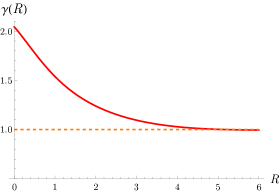
Figure 3: The interpolating function $\gamma(R)$ giving the appropriate scaling of the electron wave function as the inter-nucleon distance $R$ is varied. The right hand figure shows its first four derivatives (in order cyan, brown, orange, blue dashed) in the vicinity of the minimum of the potential at $R_{0}=2.003$.

Given $\gamma(R)$, the energy and momentum expectation values are found from (134) and (133). These are shown in Figs. 4 and 5, A few comments are worth making here. Note that the energy $E_{e}(R)$ has a deeper minimum with the improved ansatz with the interpolating function $\gamma(R)$, and it occurs at the smaller value $R_{0}=2.003$. This gives a much improved agreement with the measured dissociation energy for ${\rm H}_{2}^{+}$, though still not sufficiently deep. However, the value for the fundamental vibration frequency $\omega_{0}=\sqrt{V_{M}^{{}^{\prime\prime}}(R_{0})/\mu}=0.020\,R_{H}$, in good agreement with the measured value.

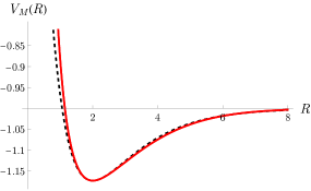
Figure 4: The nucleon potential $V_{M}(R)\equiv E_{e}(R)$ as the inter-nucleon distance, or bond length, $R$ is varied. The minimum is at $R_{0}=2.003$. The left hand figure shows a comparison with the equivalent with the scaling factor $\gamma(R)$ left fixed equal to 1 (orange, dashed). The right hand figure shows the comparison with a Morse potential (black, dashed) with its two free parameters set to match the potential minimum $V_{M}(R_{0}$ and curvature $V_{M}^{{}^{\prime\prime}}(R_{0})$.

As expected, for large $R$ where the molecule has effectively separated, $E_{e}(R)$ tends to the atomic $1s$ level $\hat{E}_{1s}=-1$. Moreover, we numerically confirm the analytic results $K(R)\rightarrow 1$ and $U(R)\rightarrow-2$ as $R\rightarrow\infty$, in agreement with the virial theorem for a Coulomb interaction. On the other hand, for $R\rightarrow 0$, if we set aside the divergent nucleon-nucleon interaction term $2/R$ in the potential, we find with $\gamma(0)=2$ that $K(0)\rightarrow 4$ and $U(0)\rightarrow-8$, again satisfying the virial theorem and confirmed numerically in Fig. 4. A comparison of $V_{M}(R)$ with the phenomenological Morse potential is also shown in Fig. 4.

We can also check the asymptotic behaviour of the momentum expectation values analytically. For both large and small $R$, where the molecule becomes effectively an atom, spherical symmetry is restored so all the expectation values in (130) and (131) are equal, with $\langle p^{a}p^{a}\rangle=\langle p^{2}\rangle/3=K/3$. This is confirmed numerically in Fig. 5 where we observe all the $\langle p^{a}p^{a}\rangle$ becoming equal and tending to $1/3$ for $R\rightarrow\infty$ and $4/3$ for $R\rightarrow 0$.

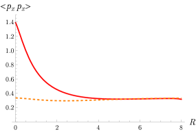
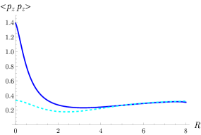
Figure 5: The momentum expectation values from (130), (131) and (133) as a function of the bond length $R$. The left hand figure shows $\langle p^{x}\,p^{x}\rangle$ evaluated with $\gamma(R)$ and (dashed curve) fixed equal to 1. The right hand figure is the same for $\langle p^{z}\,p^{z}\rangle$.

Derivative		0		1		2		3		4
$V_{M}$		-1.173		0		0.187		-0.492		1.237
$\langle p^{x}\,p^{x}\rangle$		0.451		-0.146		0.146		-0.162		0.229
$\langle p^{z}\,p^{z}\rangle$		0.271		-0.083		0.133		-0.188		0.349
$\gamma$		1.238		-0.203		0.148		-0.113		0.102
${\rm tr}\,\langle p^{a}\,p^{b}\rangle$		1.173		-0.375		0.424		-0.512		0.808
${\rm tr}_{Y}\langle p^{a}\,p^{b}\rangle$		0.360		-0.126		0.026		0.052		-0.239

Table 1: The values and first few derivatives of the inter-nucleon potential $V_{M}(R)$, the momentum expectation values $\langle p^{x}\,p^{x}\rangle$ and $\langle p^{z}\,p^{z}\rangle$, and the interpolating function $\gamma(R)$ used in their construction, all evaluated at the minimum $R_{0}=2.003$ of $V_{M}(R)$. All numbers are expressed in atomic units, with energies in terms of the reduced Rydberg constant $\hat{R}_{H}$ and lengths in terms of the reduced Bohr radius $\hat{a}_{0}$.

Finally, for the analysis of the rovibrational levels in sections 5 and 6, we need explicit values for the first few derivatives of the energy and momentum expectation values at the minimum $R_{0}$ of the improved potential $V_{M}(R)=E_{e}(R)$. These are evaluated numerically from the functions plotted above, and the required values are shown in Table 1, which may be compared with Muller:2004tc . Recall that cylindrical symmetry ensures that $\langle p^{x}\,p^{x}\rangle\,=\,\langle p^{y}\,p^{y}\rangle$. We also include here the combinations ${\rm tr}\,\langle p^{a}\,p^{b}\rangle\,=\,\langle p^{x}\,p^{x}\rangle+\langle p^{y}\,p^{y}\rangle+\langle p^{z}\,p^{z}\rangle$ and ${\rm tr}_{Y}\langle p^{a}\,p^{b}\rangle\,=\,\langle p^{x}\,p^{x}\rangle+\langle p^{y}\,p^{y}\rangle-2\langle p^{z}\,p^{z}\rangle$ which appear as coefficients in the SME potential $V_{\rm SME}^{e}$.

Appendix B Rovibrational energy levels - perturbation method

In this appendix, we present a systematic perurbative method to evaluate the rovibrational energy levels incorporating the Lorentz and CPT violating corrections. This provides an important consistency check on the results obtained in section 4.

The idea is to expand all the contributions to the potential in the nucleon Schrödinger equation (18) about the minimum $R_{0}$ of the inter-nucleon potential $V_{M}(R)$, then evaluate the energy corrections as perturbations about the leading SHO approximation. As we see, this turns out to give a systematic perturbative expansion in the small parameter $\lambda=1/\mu\,\omega_{0}R_{0}^{2}\,$ identified previously. We therefore write,

$$V_{M}(R)\,+\ V_{N}(R)\,+\,V_{\rm SME}^{e}(R)$$

$$~~=\,V_{M}(R_{0})\,+\,V_{N}(R_{0})\,+\,V_{\rm SME}^{e}(R_{0})\,+\,\frac{1}{2}\mu\omega_{0}^{2}x^{2}\,+\,\delta V_{M}(x)\,+\,\delta V_{N}(x)\,+\,\delta V_{\rm SME}^{e}(x)\ ,$$ (135)

where here $x=R-R_{0}$ and $V_{N}(R)=N(N+1)/2\mu R^{2}$, so $V_{N}(R_{0})=\tfrac{1}{2}\lambda\omega_{0}N(N+1)$. Then,

$$\delta V_{M}\, =\,\frac{1}{6}V_{M}^{{}^{\prime\prime\prime}}\,x^{3}\,+\,\frac{1}{24}V_{M}^{(4)}\,x^{4}\,+\,\ldots$$

$$\delta V_{N}\, =\,\lambda\omega_{0}N(N+1)\Big{(}-\frac{x}{R_{0}}\,+\,\frac{3}{2}\Big{(}\frac{x}{R_{0}}\Big{)}^{2}\,-\,2\Big{(}\frac{x}{R_{0}}\Big{)}^{3}\,+\,\ldots\Big{)}$$

$$\delta V_{\rm SME}^{e}\, =\,V_{\rm SME}^{e\,^{\prime}}\,x\,+\,\frac{1}{2}V_{\rm SME}^{e\,^{\prime\prime}}\,x^{2}\,+\,\frac{1}{6}V_{\rm SME}^{e\,^{\prime\prime\prime}}\,x^{3}\,+\,\ldots$$ (136)

We start from the SHO with potential $\tfrac{1}{2}V_{M}^{{}^{\prime\prime}}x^{2}\,=\,\tfrac{1}{2}\mu\,\omega_{0}^{2}\,x^{2}$ and construct the usual states labelled by integers $|v\rangle$ with energy eigenvalues $E_{v}^{(0)}=(v+\tfrac{1}{2})\omega_{0}$. We will need the expressions for the energy levels up to 3rd order in perturbation theory, viz.

$$E_{v}\,=\,E_{v}^{(0)}\,+\,E_{v}^{(1)}\,+\,E_{v}^{(2)}\,+\,E_{v}^{(3)}\ ,$$ (137)

with, for a perturbation $\delta V$ in the potential,

$$E_{v}^{(1)}\, =\,\langle v|\,\delta V\,|v\rangle\ ,$$

$$E_{v}^{(2)}\, =\,\sum_{k\neq v}\,\frac{1}{(E_{v}^{(0)}-E_{k}^{(0)})}\,\,\langle v|\,\delta V\,|k\rangle\,\,\langle k|\,\delta V\,|v\rangle\ ,$$

$$E_{v}^{(3)}\, =\,\sum_{k\neq v}\sum_{\ell\neq v}\,\frac{1}{(E_{v}^{(0)}-E_{k}^{(0)})(E_{v}^{(0)}-E_{\ell}^{(0)})}\,\,\langle v|\,\delta V\,|k\rangle\,\,\langle k|\,\delta V\,|\ell\rangle\,\,\langle\ell|\,\delta V\,|v\rangle$$

$$~~~~-\,\sum_{k\neq v}\,\frac{1}{(E_{v}^{(0)}-E_{k}^{(0)})^{2}}\,\,|\langle v|\,\delta V\,|k\rangle|^{2}\,\,\langle v|\,\delta V\,|v\rangle\,~\ .$$ (138)

The states here are all understood to be the unperturbed SHO states; clearly the notation with states carrying a label $|v\rangle^{(0)}$ throughout is too cumbersome. The perturbation $\delta V$ in our case is the sum of the anharmonic potential, angular momentum and SME terms in (4), $\delta V\,=\,\delta V_{M}\,+\,\delta V_{N}\,+\,\delta V_{\rm SME}^{e}$.

Now at first order, only even powers of $x$ contribute to the expectation values, so we have,

$$E_{v}^{(1)}\,=\,\Big{(}\frac{3}{2}\lambda\,\omega_{0}\,N(N+1)/R_{0}^{2}\,+\,\frac{1}{2}\,V_{\rm SME}^{e\,^{\prime\prime}}\,\Big{)}\,\langle v|\,x^{2}\,|v\rangle\,\,+\,\,\frac{1}{24}\,\big{(}V_{M}^{(4)}\,+\,V_{\rm SME}^{e\,(4)}\big{)}\,\langle v|\,x^{4}\,|v\rangle\ .$$ (139)

The expectation values here and throughout this section are evaluated using elementary methods, expanding the powers of $x$ in terms of raising and lowering operators using,

$$\frac{1}{R_{0}}\,x\,=\,\sqrt{\frac{\lambda}{2}}\,\,(a\,+\,a^{\dagger})~~~~~~\textrm{with}~~~~~~a^{\dagger}|v\rangle\,=\,\sqrt{v+1}\,\,|v+1\rangle\ ,~~~~a|v\rangle\,=\,\sqrt{v}\,\,|v-1\rangle\ .\\$$ (140)

Then, evaluating

$$\frac{1}{R_{0}^{2}}\langle v|\,x^{2}\,|v\rangle\,=\,(v+\tfrac{1}{2})\,\lambda\ ,~~~~~~~\textrm{and}~~~~~~\frac{1}{R_{0}^{4}}\,\langle v|\,x^{4}\,|v\rangle\,=\,\frac{3}{2}\Big{(}\,(v+\tfrac{1}{2})^{2}\,+\,\tfrac{1}{4}\Big{)}\,\lambda^{2}\ ,$$ (141)

and dropping the constant term, which adds negligibly to $V_{M}(R_{0})$, $V_{\rm SME}^{e}(R_{0})$ and the dissociation energy, we find

$$E_{v}^{(1)}\, =\,\frac{3}{2}\,(v+\tfrac{1}{2})\,N(N+1)\,\lambda^{2}\,\omega_{0}~+~\frac{1}{2}(v+\tfrac{1}{2})\,\frac{1}{V_{M}^{{}^{\prime\prime}}}\,\,V_{\rm SME}^{e\,^{\prime\prime}}\,\,\omega_{0}$$

$$~~~~+\,\frac{1}{16}\,(v+\tfrac{1}{2})^{2}\,\,\frac{1}{V_{M}^{{}^{\prime\prime}}}\,R_{0}^{2}\,\big{(}V_{M}^{(4)}\,+\,V_{\rm SME}^{e\,(4)}\,\big{)}\,\,\lambda\,\omega_{0}\ .$$ (142)

We identify these as contributions to the coefficients $\alpha_{0}$, $\,\delta_{SME}^{e}\,$ and $x_{0}$, $x_{\rm SME}^{e}$ respectively in section 5.

Next, consider the perturbations at 2nd order. Organising by the total number of factors of $x$ occurring (recalling that each power of $x$ carries an associated $\sqrt{\lambda}$), we first find contributions in (138) where both factors of $\delta V$ are proportional to $x$; then where both $\delta V\sim x^{2}$, together with a mixed term with one factor of $\delta V\sim x$ and the other $\delta V\sim x^{3}$; and finally, terms with $\delta V\sim x,\,\delta V\sim x^{5}$, $\,\delta V\sim x^{2},\,\delta V\sim x^{4}$ and both $\delta V\sim x^{3}$, the latter three contributing leading $O(\lambda)$ terms to $x_{0}$ and $x_{\rm SME}^{e}$.

Taking these in turn, we first evaluate the contribution to $E_{v}^{(2)}$ from taking the perturbation $\delta V=\Big{(}-\lambda\,\omega_{0}\,N(N+1)\,+\,R_{0}\,V_{\rm SME}^{e\,^{\prime}}\Big{)}x/R_{0}$. The required expectation value is

$$\sum_{k\neq v}\,\frac{1}{(E_{v}^{(0)}-E_{k}^{(0)})}\,\frac{1}{R_{0}^{2}}\,\langle v|\,x\,|k\rangle\,\,\langle k|\,x\,|v\rangle\,=\,-\frac{1}{2}\,\frac{1}{\big{(}R_{0}^{2}\,V_{M}^{{}^{\prime\prime}}\big{)}}\ ,$$ (143)

with the sum over $k=v\pm 1$. Notice that this is independent of the vibrational quantum number $v$. The corresponding contribution to $E_{v}^{(2)}$ is therefore

$$E_{v;\,[1,1]}^{(2)}\,=\,-\frac{1}{2}\,\lambda^{3}\,(N(N+1))^{2}\,\omega_{0}~+~\lambda\,N(N+1)\,\frac{1}{\big{(}R_{0}\,V_{M}^{{}^{\prime\prime}}\big{)}}\,V_{\rm SME}^{e\,^{\prime}}\,\,\omega_{0}\ ,$$ (144)

which we identify with terms in $D_{0}$ and $B_{\rm SME}^{e}$ respectively.

A similar calculation shows

$$\sum_{k\neq v}\,\frac{1}{(E_{v}^{(0)}-E_{k}^{(0)})}\,\frac{1}{R_{0}^{4}}\,\langle v|\,x\,|k\rangle\,\,\langle k|\,x^{3}\,|v\rangle\,=\,-\frac{3}{2}\,\lambda\,\frac{1}{\big{(}R_{0}^{2}\,V_{M}^{{}^{\prime\prime}}\big{)}}\,(v+\tfrac{1}{2})\ ,$$ (145)

and identifying the relevant perturbations $\delta V$ from (136) we find

$$E_{v;\,[1,3]}^{(2)}\, =\,-\frac{1}{2}\,(v+\tfrac{1}{2})\,\frac{V_{M}^{{}^{\prime\prime\prime}}}{\big{(}V_{M}^{{}^{\prime\prime}}\bigr{)}^{2}}\,V_{\rm SME}^{e\,^{\prime}}\,\,\omega_{0}~+~\frac{1}{2}\,\lambda^{2}\,(v+\tfrac{1}{2})\,N(N+1)\,\frac{R_{0}\,V_{M}^{{}^{\prime\prime\prime}}}{V_{M}^{{}^{\prime\prime}}}\,\omega_{0}$$

$$~~~~~~~+\,\lambda^{2}\,(v+\tfrac{1}{2})\,N(N+1)\,\Big{(}\frac{1}{2}\frac{R_{0}}{V_{M}^{{}^{\prime\prime}}}\,\,V_{\rm SME}^{e\,^{\prime\prime\prime}}\,+\,6\frac{1}{\big{(}R_{0}\,V_{M}^{{}^{\prime\prime}}\big{)}}\,V_{\rm SME}^{e\,^{\prime}}\,\Big{)}\,\,\omega_{0}\ .$$ (146)

These are contributions to $\delta_{\rm SME}^{e}$, $\alpha_{0}$ and $\alpha_{\rm SME}^{e}$ respectively.

The next contribution at 2nd order comes from terms where both $\delta V\sim x^{2}$, so here we need to calculate

$$\sum_{k\neq v}\,\frac{1}{(E_{v}^{(0)}-E_{k}^{(0)})}\,\frac{1}{R_{0}^{4}}\,\langle v|\,x^{2}\,|k\rangle\,\,\langle k|\,x^{2}\,|v\rangle\,=\,-\frac{1}{2}\,\lambda\,\frac{1}{\big{(}R_{0}^{2}\,V_{M}^{{}^{\prime\prime}}\big{)}}\,(v+\tfrac{1}{2})\ ,$$ (147)

giving the energy

$$E_{v;\,[2,2]}^{(2)}\,=\,-\frac{3}{4}\,\lambda^{2}\,(v+\tfrac{1}{2})\,N(N+1)\,\frac{1}{V_{M}^{{}^{\prime\prime}}}\,V_{\rm SME}^{e\,^{\prime\prime}}\,\,\omega_{0}\ ,$$ (148)

which adds to $\alpha_{\rm SME}^{e}$. We have discarded the $\lambda^{4}\,(v+\tfrac{1}{2})\,\big{(}N(N+1)\big{)}^{2}\omega_{0}$ term here as it is not of the type for which we have kept the coefficients in (56).

Moving on to the 2nd order contributions with a total of 6 powers of $x$, we find they involve factors of $(v+\tfrac{1}{2})^{2}$, so we are only concerned here with their effect on $x_{0}$ and $x_{\rm SME}^{e}$. In turn, these are:

$$\sum_{k\neq v}\,\frac{1}{(E_{v}^{(0)}-E_{k}^{(0)})}\,\frac{1}{R_{0}^{6}}\,\langle v|\,x^{3}\,|k\rangle\,\,\langle k|\,x^{3}\,|v\rangle\,=\,-\frac{15}{4}\,\lambda\,\omega_{0}\,\big{[}(v+\tfrac{1}{2})^{2}\,+\,\tfrac{7}{60}\big{]}\,\frac{1}{\big{(}R_{0}^{2}\,V_{M}^{{}^{\prime\prime}}\big{)}^{2}}\ ,$$ (149)

from which,

$$E_{v;\,[3,3]}^{(2)}\,=\,-\frac{5}{48}\,\lambda\,\omega_{0}\,\big{[}(v+\tfrac{1}{2})^{2}\,+\,\tfrac{7}{60}\big{]}\,\frac{1}{V_{M}^{{}^{\prime\prime}}}\,R_{0}^{2}\,\big{(}(V_{M}^{{}^{\prime\prime\prime}})^{2}\,+\,2V_{M}^{{}^{\prime\prime\prime}}\,V_{\rm SME}^{e\,^{\prime\prime\prime}}\big{)}\ ,$$ (150)

contributing to $x_{0}$ and $x_{\rm SME}^{e}$;

$$\sum_{k\neq v}\,\frac{1}{(E_{v}^{(0)}-E_{k}^{(0)})}\,\frac{1}{R_{0}^{6}}\,\langle v|\,x^{2}\,|k\rangle\,\,\langle k|\,x^{4}\,|v\rangle\,=\,-\frac{3}{2}\,\lambda\,\omega_{0}\,\big{[}(v+\tfrac{1}{2})^{2}\,+\,\tfrac{1}{4}\big{]}\,\frac{1}{\big{(}R_{0}^{2}\,V_{M}^{{}^{\prime\prime}}\big{)}^{2}}\ ,$$ (151)

giving

$$E_{v;\,[2,4]}^{(2)}\,=\,-\frac{1}{16}\,\lambda\,\omega_{0}\,\big{[}(v+\tfrac{1}{2})^{2}\,+\,\tfrac{1}{4}\big{]}\,\frac{1}{\big{(}V_{M}^{{}^{\prime\prime}}\big{)}^{2}}\,R_{0}^{2}\,V_{M}^{(4)}\,V_{\rm SME}^{e\,^{\prime\prime}}\ ,$$ (152)

which contributes only to $x_{\rm SME}^{e}$; and

$$\sum_{k\neq v}\,\frac{1}{(E_{v}^{(0)}-E_{k}^{(0)})}\,\frac{1}{R_{0}^{6}}\,\langle v|\,x\,|k\rangle\,\,\langle k|\,x^{5}\,|v\rangle\,=\,-\frac{15}{4}\,\lambda\,\omega_{0}\,\big{[}(v+\tfrac{1}{2})^{2}\,+\,\tfrac{1}{4}\big{]}\,\frac{1}{\big{(}R_{0}^{2}\,V_{M}^{{}^{\prime\prime}}\big{)}^{2}}\ ,$$ (153)

giving

$$E_{v;\,[1,5]}^{(2)}\,=\,-\frac{1}{16}\,\lambda\,\omega_{0}\,\big{[}(v+\tfrac{1}{2})^{2}\,+\,\tfrac{1}{4}\big{]}\,\frac{1}{\big{(}V_{M}^{{}^{\prime\prime}}\big{)}^{2}}\,R_{0}^{2}\,V_{M}^{(5)}\,V_{\rm SME}^{e\,^{\prime}}\ ,$$ (154)

which again only contributes to $x_{\rm SME}$. Comparing with (57) and (67), we see that we have now reproduced exactly all the terms found in the effective potential method up to 2nd order in the perturbations.

So far, in (141) and (149), (151), (153), we have just discussed the $O(v+\tfrac{1}{2})^{2}$ contributions, keeping only the terms independent of the angular momentum since we dropthese at $O\big{(}(v+\tfrac{1}{2})^{2}N(N+1)\big{)}$. However, the constant factors do contribute to $B_{0}$, $B_{\rm SME}^{e}$ and $D_{0}$, though not $D_{\rm SME}^{e}$ since this only receives contributions at 3rd order (see below). Inspecting these terms, we see that they give sub-leading contributions, of $O(\lambda^{3})$ in $B_{0}$ and $B_{\rm SME}^{e}$ and $O(\lambda^{5})$ in $D_{0}$, picking up all the terms of 2nd order, but only 2nd order, in the perturbations. This confirms that in (57), $B_{0}=\frac{1}{2}\lambda\,+\,O(\lambda^{3})$ is a power series in $\lambda^{2}$ with leading term of $O(\lambda)$, with an analogous result for $B_{\rm SME}^{e}$ and $D_{0}$.

Evidently we can continue straightforwardly to as many orders as desired, though of course evaluating the products of expectation values becomes increasingly laborious. It is interesting however to display just one term at 3rd order, which gives the leading term to the coefficient $D_{\rm SME}^{e}$. In this case we need two factors of $\delta V\sim x$ and one $\delta V\sim x^{2}$ and from (138) the required calculation is

$$\sum_{k\neq v}\sum_{\ell\neq v}\,\frac{1}{(E_{v}^{(0)}-E_{k}^{(0)})(E_{v}^{(0)}-E_{\ell}^{(0)})}\,\,\frac{1}{R_{0}^{4}}\,\Big{[}\langle v|\,x\,|k\rangle\,\,\langle k|\,x^{2}\,|\ell\rangle\,\,\langle\ell|\,x\,|v\rangle$$

$$~~~~~~~~~~~~~~~~~~~~~~~~~~~~~~~~~~~~~~~~~~~~~~~~~~~~~~~~~~~~~~~~~~\,+\,2\,\langle v|\,x\,|k\rangle\,\,\langle k|\,x\,|\ell\rangle\,\,\langle\ell|\,x^{2}\,|v\rangle\,\Big{]}$$

$$~~-\sum_{k\neq v}\,\frac{1}{(E_{v}^{(0)}-E_{k}^{(0)})^{2}}\,\,\frac{1}{R_{0}^{4}}\,\langle v|\,x\,|k\rangle\,\,\langle k|\,x\,|v\rangle\,\,\langle v|\,x^{2}\,|v\rangle$$

$$=\,\,\frac{1}{4}\,\frac{1}{\big{(}R_{0}^{2}V_{M}^{{}^{\prime\prime}}\big{)}^{2}}\,\,\Big{[}\big{(}2(v+\tfrac{1}{2})^{2}+\tfrac{5}{2}\big{)}\,+\,2\big{(}(v+\tfrac{1}{2})^{2}+\tfrac{3}{4}\big{)}\,-\,4(v+\tfrac{1}{2})^{2}\Big{]}$$

$$=\,\,\frac{1}{\big{(}R_{0}^{2}V_{M}^{{}^{\prime\prime}}\big{)}^{2}}\ .$$ (155)

Remarkably, the terms of $O(v+\tfrac{1}{2})^{2}$ cancel, leaving a residual $v$-independent term, as required to contribute to the $D_{\rm SME}^{e}$ coefficient. Then, since we can select terms with both $\delta V_{\rm SME}^{e}\sim x^{2},\,\delta V_{N}\sim x,\,\delta V_{N}\sim x$ and $\delta V_{\rm SME}^{e}\sim x,\,\delta V_{N}\sim x,\,\delta V_{N}\sim x^{2}$, we identify the required contribution to $E_{v}^{(3)}$:

$$E_{v}^{(3)}\,=\,\lambda^{3}\,\big{(}(N(N+1)\big{)}^{2}\,\,\bigg{[}\,\frac{1}{2}\frac{1}{V_{M}^{{}^{\prime\prime}}}\,V_{\rm SME}^{e\,^{\prime\prime}}\,-\,3\frac{1}{\big{(}R_{0}\,V_{M}^{{}^{\prime\prime}}\big{)}}\,V_{\rm SME}^{e\,^{\prime}}\,\bigg{]}\,\omega_{0}~~~\ldots$$ (156)

This is to be compared with (66) calculated with the effective potential method.

A careful comparison of these results with those derived by the effective potential method in section 5 shows that apart from (156) we have yet to identify the terms in (57) and (66),(67) involving more than two perturbative factors, frequently involving higher derivatives of the potential $V_{M}(R)$. To compare the origin of these terms in the effective potential and perturbation theory methods, and to verify that the terms quoted in section 5 for the rovibrational energies are complete at the quoted order in $\lambda$, we need to analyse more closely the systematics of the expansion in $\lambda$ in this expectation value approach.

First, notice that in the perturbation series in (138), each power of $x$ in the perturbations $\delta V$ brings a factor of $\sqrt{\lambda}$ from its expression (140) in raising and lowering operators. Then from the energy denominators, each further order in $\delta V$ brings with it an extra factor of $1/\omega_{0}=1/(R_{0}^{2}\,V_{M}^{{}^{\prime\prime}}\,\lambda)$.

We can therefore count the relevant orders by inspection. For example, consider the $D_{0}$ coefficient. This arises first at 2nd order from (11) with both $\delta V_{N}\sim x$, so the expectation value itself is $O(\lambda/\omega_{0}$ and since $\delta V_{N}$ itself is of $O(\lambda\omega_{0}$, the corresponding energy is $O(\lambda^{3}\omega_{0})$. Remembering to extract a factor $w_{0}$ to leave the coefficient $D_{0}$ dimensionless, we deduce immediately that $D_{0}\sim\lambda^{3}$, as given in (11.

The next contribution would come from including the $O(x^{3})$ term in the expansion of one of the $\delta V_{N}$ factors. But then the expectation value would be $O(\lambda^{2}/\omega_{0}$ and the contribution to $D_{0}$ would be $O(\lambda^{4}$. We see therefore that as already indicated, the coefficient $D_{0}$ quoted in (11) is the leading term in a perturbative series in the small parameter $\lambda$. The same is true of all the rovibrational energy coefficients.

We can now use this power counting to understand the origin of the factors involving higher derivatives of $V_{M}(R)$ and why they must be included. A good example is $\alpha_{0}$. As we have seen above, this arises already in 1st order with $\delta V_{N}\sim\lambda\omega_{0}x^{2}$. The expectation value $\langle x^{2}\langle$ is $O(\lambda)$, so we find the $E_{v}^{(1)}$ contribution is $O(\lambda^{2}\omega_{0}$, giving $\alpha_{0}\sim\lambda^{2}$. However, from (11) we know that this is not the complete result for $\alpha_{0}$ which has another contribution of the same $O(\lambda^{2})$ but with a factor depending on $V_{M}^{{}^{\prime\prime\prime}}$. This arises at 2nd order, with perturbations $\delta V_{N}\sim\lambda\,\omega_{0}x$ and $\delta V_{M}\sim V_{M}^{{}^{\prime\prime\prime}}\,x^{3}$. Following the power counting rules, this $E_{v}^{(2)}$ contribution is $O(\lambda^{2}\omega_{0}V_{M}^{{}^{\prime\prime\prime}}/V_{M}^{{}^{\prime\prime}})$, giving the complete $O(\lambda^{2})$ result for $\alpha_{0}$ found in (11).

What this example shows us is that in general we can find another contribution to a particular rovibrational coefficient which is of the same order in $\lambda$ by going to a higher order in the SHO perturbation series (138) and including a correspondingly higher derivative term in the expansion of $\delta V_{M}$ if (and only if) at the same time we can reduce the power of $x$ from the expansion of the perturbation $\delta V_{N}$ or $\delta V_{\rm SME}$ which specifies that coefficient. This process can obviously not be iterated indefinitely and this is why the number of terms in a rovibrational coefficient at a given order in $\lambda$ is limited.

These considerations allow us to identify the perturbative origin of all the terms in the rovibrational coefficients quoted in section 5 and to verify that they are indeed complete. Notice also that the effective potential method, where we analyse the anharmonic oscillator around the minimum of the potential including the perturbations, is in some ways more efficient in identifying terms that otherwise require high orders in the systematic perturbation method.

References

- (1) W. Pauli, Phys. Rev. 58 (1940) 716.
- (2) J. S. Bell, Birmingham University thesis (1954).
- (3) G. Lüders, Det. Kong. Danske Videnskabernes Selskab Mat. fysiske Meddelelser 28 (1954) no. 5.
- (4) W. Pauli, in W. Pauli, ed., “Niels Bohr and the Development of Physics”, McGraw-Hill, New York, 1955.
- (5) M. Charlton, S. Eriksson and G. M. Shore, “Antihydrogen and Fundamental Physics”, Springer, 2020; preprint [arXiv:2002.09348 [hep-ph]].
- (6) M. J. Borchert et al. [BASE], “A 16-parts-per-trillion measurement of the antiproton-to-proton charge–mass ratio”, Nature 601 (2022), 53.
- (7) M. Ahmadi et al. [ALPHA], “Characterization of the - transition in antihydrogen”, Nature 557 (2018), 71.
- (8) M. Ahmadi et al. [ALPHA], “Observation of the hyperfine spectrum of antihydrogen”, Nature 548 (2017), 66.
- (9) M. Ahmadi et al. [ALPHA], “Investigation of the fine structure of antihydrogen”, Nature 578 (2020), 375. [erratum: Nature 594 (2021), E5]
- (10) M. Ahmadi et al. [ALPHA], “Observation of the - transition in trapped antihydrogen”, Nature 541 (2016), 506-510
- (11) H. Muller, S. Herrmann, A. Saenz, A. Peters and C. Lammerzahl, “Tests of Lorentz invariance using hydrogen molecules”, Phys. Rev. D 70 (2004), 076004.
- (12) S. Schiller, “Precision Spectroscopy of molecular hydrogen ions: an introduction”, Contemporary Physics 63 (2022), 247 and Supplementary material.
- (13) A. Carrington et al, “Spectroscopy of the hydrogen molecular ion”, J. Phys. B: At. Mol. Opt. Phys. 22 (1989) 3551.
- (14) S. Schiller, D. Bakalov and V. I. Korobov, “Simplest Molecules as Candidates for Precise Optical Clocks”, Phys. Rev. Lett. 113 (2014), 023004.
- (15) M. R. Schenkel, S. Alinghanbari and S. Schiller, “Laser spectroscopy of a rovibrational transition in the molecular hydrogen ion ”, Nature Physics 20 (2024), 383.
- (16) D. Colladay and V. A. Kostelecky, “Lorentz violating extension of the standard model”, Phys. Rev. D 58 (1998), 116002. [arXiv:hep-ph/9809521 [hep-ph]].
- (17) A. Kostelecký and M. Mewes, “Fermions with Lorentz-violating operators of arbitrary dimension”, Phys. Rev. D 88 (2013), 096006. [arXiv:1308.4973 [hep-ph]].
- (18) V. A. Kostelecky and N. Russell, “Data Tables for Lorentz and CPT Violation”, Rev. Mod. Phys. 83 (2011), 11. [arXiv:0801.0287v17 [hep-ph]].
- (19) V. A. Kostelecký and A. J. Vargas, “Lorentz and CPT tests with hydrogen, antihydrogen, and related systems”, Phys. Rev. D 92 (2015), 056002. [arXiv:1506.01706 [hep-ph]].
- (20) A. Berera and L. Del Debbio, “Quantum Mechanics”, Cambridge University Press, 2022.
- (21) D. A. Varshalovich and A. V. Sannikov, “ molecular ions in the interstellar medium”, Pis’ma Astron. Zh. 19 (1993), 719.
- (22) V. I. Korobov, “Rovibrational states of . Variational calculations”, Molecular Physics 116 (2017), 93. Erratum: Mol. Phys. 119 (12) (2021).
- (23) V. A. Kostelecky and C. D. Lane, “Nonrelativistic quantum Hamiltonian for Lorentz violation”, J. Math. Phys. 40 (1999), 6245. [arXiv:hep-ph/9909542 [hep-ph]].
- (24) T. J. Yoder and G. S. Adkins, “Higher order corrections to the hydrogen spectrum from the Standard-Model Extension”, Phys. Rev. D 86 (2012), 116005. [arXiv:1211.3018 [hep-ph]].
- (25) S. Alighanbari, G. S. Giri, F L. Constantin, V. I. Korobov and S. Schiller, “Precise test of quantum electrodynamics and determination of fundamental constants with ions”, Nature 581 (2020), 152.
- (26) E. G. Myers, “CPT tests with the antihydrogen molecular ion”, Phys. Rev. A 98 (2018), 010101(R).
- (27) J.-Ph. Karr, “Stark quenching of rovibrational states of due to motion in a magnetic field”’ Phys. Rev. A 98 (2018), 062501.
- (28) M. C. Zammit et al., “Laser-driven production of the antihydrogen molecular ion”, Phys. Rev. A 100 (2019) 042709.
- (29) C. G. Parthey, A. Matveev, J. Alnis, B. Bernhardt et al. “Improved Measurement of the Hydrogen 1S - 2S Transition Frequency”, Phys. Rev. Lett. 107 (2011), 203001.
- (30) A. Matveev, C. G. Parthey, K. Predehl et al. “Precision Measurement of the Hydrogen 1S2S Frequency via a 920-km Fiber Link”, Phys. Rev. Lett. 110 (2013), 230801.
- (31) V. I. Korobov, L. Hilico and J.-Ph. Karr, “Hyperfine structure in the hydrogen molecular ion”, Phys. Rev. A 74 (2006), 040502(R).
- (32) J.-Ph. Karr, V. I. Korobov and L. Hilico, “Vibrational spectroscopy of : Precise evaluation of the Zeeman effect”, Phys. Rev. A 77 (2008), 062507.
- (33) J.-Ph. Karr, V. I. Korobov and L. Hilico, “Vibrational spectroscopy of : Hyperfine structure of two-photon transitions”, Phys. Rev. A 77 (2008), 063410.