Deformations of Kalck–Karmazyn algebras
via Mirror Symmetry

Abstract.

As observed by Kawamata [13], a $\mathbb{Q}$-Gorenstein smoothing of a Wahl singularity gives rise to a one-parameter flat degeneration of a matrix algebra. A similar result holds for a general smoothing of any two-dimensional cyclic quotient singularity, where the matrix algebra is replaced by a hereditary algebra [24]. From a categorical perspective, these one-parameter families of finite-dimensional algebras ”absorb” the singularities of the threefold total spaces of smoothings. These results were established using abstract methods of birational geometry, making the explicit computation of the family of algebras challenging. Using mirror symmetry for genus-one fibrations [16], we identify a remarkable immersed Lagrangian with a bounding cochain in the punctured torus. The endomorphism algebra of this Lagrangian in the relative Fukaya category corresponds to this flat family of algebras. This enables us to compute Kawamata’s matrix order explicitly.

1. Introduction

The notion of singularity category [4, 20] provides a direct way to compare module categories of rings of dissimilar nature, such as the local rings of singular algebraic varieties and finite-dimensional algebras. Sometimes one can even find an algebra $\mathcal{R}$ that “absorbs” [15] singularities of an algebraic variety $\mathcal{W}$, i.e., there exists a semi-orthogonal decomposition $D^{b}(\mathcal{W})=\langle D^{b}(\mathcal{R}),\mathcal{B}\rangle$ such that $\mathcal{B}\subset\mathrm{Perf}(\mathcal{W})$. The algebra $\mathcal{R}$ is typically presented as the endomorphism algebra of some object in $D^{b}(\mathcal{W})$, such as a vector bundle on $\mathcal{W}$. The goal of this paper is to demonstrate that homological mirror symmetry can help to compute the algebra $\mathcal{R}$ explicitly.

Consider a cyclic quotient singularity $\mathbb{A}^{2}/\mu_{r}$, where the primitive root of unity $\zeta\in\mu_{r}$ acts on $\mathbb{A}^{2}$ with weights $(\zeta,\zeta^{a})$, and $a$ and $r$ are coprime. This singularity, denoted by ${1\over r}(1,a)$, is absorbed, after an appropriate compactification, by an $r$-dimensional algebra $R_{r,a}$ called the Kalck–Karmazyn algebra [9, 11].

For example, the singularity ${1\over 4}(1,1)$ (the cone over the rational normal curve of degree $4$) is absorbed by the $4$-dimensional algebra $R_{4,1}=k[x,y,z]/(x,y,z)^{2}$. In general, we show that $R_{r,a}$ has a simple multiplication table; see Corollary 1.3.

A singularity of dimension $n+1$ can be viewed as the total space of a deformation of an $n$-dimensional singularity. The notion of categorical absorption is modified so that $\mathcal{R}$ is now a $B$-algebra, where $\mathop{\hbox{\rm{Spec}}}B$ is the base of the deformation. The algebra $\mathcal{R}$ was constructed for general deformations of ${1\over r}(1,a)$ in [24]. It is flat over $B$ and has the Kalck–Karmazyn algebra $R_{r,a}$ as the special fiber. Its general fiber is Morita-equivalent to the path algebra of an acyclic quiver. The proof is based on [13], which studied the following special case: the singularity is Wahl, i.e., $r=n^{2}$ and $a=nq-1$ for coprime $n$ and $q$, and the smoothing is $\mathbb{Q}$-Gorenstein, meaning the relative canonical divisor is $\mathbb{Q}$-Cartier. In this case, it turns out that the deformation is absorbed by a matrix order. Recall that a matrix order over, say, $B=k[t]$, is a flat $B$-algebra $\mathcal{R}$ such that $\mathcal{R}\otimes_{B}K={\mathop{\hbox{\rm{Mat}}}}_{n}(K)$, where $K=k(t)$.

Example 1.1.

Let $\mathcal{R}\subset{\mathop{\hbox{\rm{Mat}}}}_{2}(k[t])$ be a subalgebra given by elements of the form

$$\left[\small\begin{matrix}a_{0}&ta_{3}\\ {ta_{1}}&ta_{2}+a_{0}\\ \end{matrix}\right]$$ (1)

where $a_{i}\in k[t]$ for $i=0,1,2,3$. It can be verified that $\mathcal{R}$ is an order which gives a flat deformation of the $4$-dimensional algebra $R_{4,1}=k[x,y,z]/(x,y,z)^{2}$. In fact, this order corresponds to the $\mathbb{Q}$-Gorenstein smoothing of the singularity ${1\over 4}(1,1)$.

One of our main results is the calculation of a matrix order $\mathcal{R}_{n^{2},nq-1}$, which corresponds to the $\mathbb{Q}$-Gorenstein smoothing of any Wahl singularity ${1\over n^{2}}(1,nq-1)$. Before describing this order, we first explain our geometric approach.

In Section 2, we compactify the singularity ${1\over r}(1,a)$ using a projective surface $W$ and review the construction of a remarkable vector bundle $F$ on $W$ of rank $r$, called the Kawamata vector bundle. The Kalck–Karmazyn algebra $R_{r,a}$ is defined as the endomorphism algebra $\mathrm{End}(F)$. It is an $r$-dimensional $k$-algebra. The Kawamata vector bundle deforms to the vector bundle $\mathcal{F}$ on the total space $\mathcal{W}$ of any deformation of $W$, producing a flat family $\mathcal{R}=\mathrm{End}(\mathcal{F})$ of $r$-dimensional algebras.

To apply mirror symmetry, we choose a compactification $W$ that contains an anticanonical divisor $E=A\cup B$, a curve of arithmetic genus $1$. The components $A$ and $B$, both isomorphic to $\mathbb{P}^{1}$, intersect at the singular point $P$ of $W$ as the orbifold coordinate axes of $\mathbb{A}^{2}/\mu_{r}$ and at a smooth point $Q$ transversally (see Figure 1). We reduce the computation to $E$ by showing, in Lemma 2.2, that $R_{r,a}\cong\mathrm{End}(F|_{E})$.

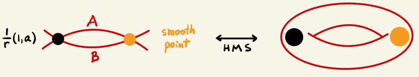
Figure 1. The divisor $E$ and its mirror, the two-punctured torus $\mathbb{T}_{2}$

Instead of computing $\mathrm{End}(F|_{E})$ directly in the perfect derived category $\mathrm{Perf}(E)$, we use homological mirror symmetry. By our construction, $E$ is a cycle of two projective lines, where the irreducible components meet transversely at two points. We write $E_{n}$ for the curve with $n$ irreducible components, each isomorphic to $\mathbb{P}^{1}$, such that the intersection complex is an $n$-gon. Homological mirror symmetry for $E_{n}$ was proven in [16] (and alternatively in [17]) as an explicit quasi-equivalence between the split-closed derived compact Fukaya category of the $n$-punctured torus $\mathbb{T}_{n}$ and the perfect derived category of $E_{n}$:

$$\mathcal{F}(\mathbb{T}_{n})\simeq\mathrm{Perf}(E_{n}).$$ (2)

Definition 1.2.

The Kawamata Lagrangian $\mathbb{K}_{r,a}\in\mathcal{F}(\mathbb{T}_{2})$ is the mirror Lagrangian of the vector bundle $F|_{E}\in\mathrm{Perf}(E_{2})$ under homological mirror symmetry.

In our calculations with Fukaya categories, we will always assume that $n\geq 1$. Since the symplectic surface $\mathbb{T}_{n}$ is punctured at least once, its symplectic form is exact, $\omega=d\lambda$, and we use the exact Fukaya category as defined in [23]. The objects of $\mathcal{F}(\mathbb{T}_{n})$ are connected, compact, and exact Lagrangians $\mathbb{L}$ (i.e., $\lambda|\mathbb{L}$ is exact) with a choice of brane data (spin structure, a $U(1)$-local system, and grading data). Changing the spin structure or local system on $\mathbb{L}$ in $\mathcal{F}(\mathbb{T}_{n})$ corresponds to tensoring the corresponding complex in $\mathrm{Perf}(E_{n})$ with a topologically trivial line bundle (equivalently, one of degree $0$ on all irreducible components of $E_{n}$), while changing the grading data corresponds to a shift in the triangulated category. In our illustrations of Lagrangians, we choose a closed curve from every homotopy class to represent the unique (up to Hamiltonian isotopy) exact Lagrangian in that class.

The Kawamata Lagrangian $\mathbb{K}_{r,a}$ is computed in Theorem 2.4 and illustrated in Figure 2, where $b$ is the inverse of $a$ modulo $r$. We represent a $2$-torus as a rectangle with opposite sides identified. Note the two punctures near the NW corner.

Figure 2. Kawamata Lagrangian $\mathbb{K}_{r,a}$ (here $r=16$, $a=3$, $b=11$)

Thus, by the definition of $\mathbb{K}_{r,a}$, we have that $\mathrm{End}(\mathbb{K}_{r,a})$ is isomorphic to the Kalck–Karmazyn algebra $R_{r,a}$. While we are mostly interested in deformations of $R_{r,a}$, our study also yields a simple multiplication table for the algebra $R_{r,a}$ itself, which was previously unknown. We find this description of $R_{r,a}$, provided below, easier to work with than its presentation by generators and relations [9, p. 3].

Corollary 1.3.

The Kalck–Karmazyn algebra $R_{r,a}$ has basis $w_{i}$ for $i\in\mathbb{Z}_{r}$ and product

$$w_{j}w_{i}=\begin{cases}w_{j+i}&\hbox{\rm if a certain condition is satisfied}\cr 0&\hbox{\rm otherwise.}\end{cases}$$ (3)

To explain the condition, let $\gamma:\,\mathbb{Z}^{2}\to\mathbb{Z}_{r}$ be a homomorphism $(i,j)\mapsto j-bi\mod r$ and consider a sublattice $\Gamma=\mathrm{Ker}(\gamma)\subset\mathbb{Z}^{2}$. We plot points of $\Gamma$ as orange dots, as they correspond to the orange puncture (see Figure 2) in the universal cover of the torus. Consider the biggest Young diagram in the first quadrant with the bottom left corner at $(0,0)$ that does not contain orange dots in its interior. We fill every box of this Young diagram with the number $\gamma(i,j)\in\mathbb{Z}_{r}$, where $(i,j)$ is the bottom left corner of the box.

To compute the product $w_{j}w_{i}$, we locate the box filled with $j$ (resp.,with $i$) in the bottom row (resp., left column) of the Young diagram. If the smallest rectangle containing these boxes is contained in the Young diagram, then $w_{j}w_{i}=w_{j+i}$. Otherwise, $w_{j}w_{i}=0$.

This description of the Kalck–Karmazyn algebra $R_{r,a}$ arises from our analysis of holomorphic polygons with boundaries on the Kawamata Lagrangian.

Example 1.4.

Suppose $r=9$ and $a=2$. Then $b=5$. From the Young diagram, the non-trivial products in $R_{9,2}$ are $w_{4}w_{1}=w_{5}$, $w_{4}w_{2}=w_{6}$, $w_{4}w_{3}=w_{7}$, and $w_{4}^{2}=w_{8}$.

Example 1.5.

$a=b=r-1$ or $a=b=1$ are the only cases when $R_{r,a}$ is a commutative algebra. Below, the first case is illustrated on the left and the second case on the right (for $r=7$). In the first case, $w_{j}w_{i}=w_{j+i}$ if and only if $j+i<r$ and so $R_{r,r-1}\cong\mathbb{Z}[t]/t^{r}$ via an isomorphism $w_{i}\mapsto t^{i}$. In the second case, $w_{j}w_{i}=w_{j+i}$ if and only if $i=0$ or $j=0$ and so $R_{r,1}\cong\mathbb{Z}[w_{1},\ldots,w_{r-1}]/(w_{1},\ldots,w_{r-1})^{2}$.

Remark 1.6.

The lattices $\Gamma$ of orange dots for singularities ${1\over r}(1,a)$ and ${1\over r}(1,b)$, where, as above, $b$ is the inverse of $a$ modulo $r$, are clearly symmetric with respect to the diagonal $y=x$. It follows that the algebras $R_{r,a}$ and $R_{r,b}$ are opposite algebras. This was also observed in [10, paragraph after Prop. 6.7].

In Section 3, we study deformations of the Kalck–Karmazyn algebra $R_{r,a}$ by endowing the Kawamata Lagrangian $\mathbb{K}_{r,a}$ with appropriate bounding cochains and computing the endomorphism algebra in the relative Fukaya category.

An obvious way to obtain a deformed object from $\mathbb{K}_{r,a}$ is to view it as an object of the relative Fukaya category $\mathcal{F}(\mathbb{T}_{1},{s})$, which deforms $\mathcal{F}(\mathbb{T}_{2})$, where the black puncture becomes a compactification divisor ${s}$. This relative category has objects represented by the same Lagrangians as in $\mathcal{F}(\mathbb{T}_{2})$; however, the $A_{\infty}$ structure is deformed due to new contributions from holomorphic polygons passing through ${s}$.

Because of the existence of bigons with boundary on $\mathbb{K}_{r,a}$ passing through $s$, this naive attempt does not yield a deformation that keeps the rank of $\mathrm{End}(\mathbb{K}_{r,a})$ constant. The idea is salvaged by equipping the Lagrangian $\mathbb{K}_{r,a}$ with a bounding cochain $\mathfrak{b}\in\mathrm{CF}^{1}(\mathbb{K}_{r,a},\mathbb{K}_{r,a})$ in $\mathcal{F}(\mathbb{T}_{1},{s})$. The coefficients of $\mathfrak{b}$ and the deformation parameter $s$ must satisfy a non-trivial equation to achieve a constant rank deformation. One of our main observations is that different choices of bounding cochains satisfying the constant rank condition correspond to the irreducible components of the versal deformation space of the cyclic quotient singularity ${1\over r}(1,a)$. This idea is made precise in Conjecture 1.9 below.

On the algebro-geometric side, we study deformations of the algebra $R_{r,a}$ to a flat $A$-algebra $\mathcal{R}={\mathop{\hbox{\rm{End}}}}(\mathcal{F})$, where $\mathcal{F}$ is a deformation of the Kawamata vector bundle $F$ to a deformation $\mathcal{W}$ of an algebraic surface $W$ over the base $\mathop{\hbox{\rm{Spec}}}A$. To apply mirror symmetry for genus-one fibrations, we assume that the divisor $E\subset W$ deforms to a divisor $\mathcal{E}\subset\mathcal{W}$ such that a general fiber $\mathcal{E}_{t}$ of the genus-one fibration $\mathcal{E}$ has one node. Starting from the divisor $E\cong E_{2}$ on $W$ (see Figure 1), we obtain the divisor $\mathcal{E}_{t}\cong E_{1}$ by smoothing the black node $P$, where $W$ is singular, while retaining the orange node $Q$, where $W$ is smooth.

We show that $\mathcal{R}\cong{\mathop{\hbox{\rm{End}}}}(\mathcal{F}|_{\mathcal{E}})$. This suggests the following strategy: first, compute deformations of the vector bundle $F_{E}$ to the total space $\mathcal{E}$ of the fibration. The versal deformation space ${\mathop{\hbox{\rm{Def}}}}_{F_{E}/\mathcal{E}}$ is smooth over $\mathop{\hbox{\rm{Spec}}}A$ with fibers isomorphic to $\mathop{\hbox{\rm{Ext}}}^{1}(F_{E},F_{E})$. In contrast to deformations of the Kawamata vector bundle on the algebraic surface, the endomorphism algebra of an arbitrary deformation of the vector bundle $F_{E}$ is typically not $A$-flat, since a deformed vector bundle will typically have an endomorphism algebra of smaller dimension than $R_{r,a}={\mathop{\hbox{\rm{End}}}}(F_{E})$.

Definition 1.7.

Let $\mathcal{V}$ be a universal vector bundle on $\mathcal{E}\times_{A}{\mathop{\hbox{\rm{Def}}}}_{F_{E}/\mathcal{E}}$. We consider a closed subset ${\mathop{\hbox{\rm{Def}}}}^{0}_{F_{E}/\mathcal{E}}\subset{\mathop{\hbox{\rm{Def}}}}_{F_{E}/\mathcal{E}}$ (with a natural subscheme structure) such that $p\in{\mathop{\hbox{\rm{Def}}}}^{0}_{F_{E}/\mathcal{E}}$ if and only if $\dim{\mathop{\hbox{\rm{End}}}}(\mathcal{V}_{p})=\dim{\mathop{\hbox{\rm{End}}}}(F_{E})$ (the maximal possible). The family of algebras ${\mathop{\hbox{\rm{End}}}}(\mathcal{V}_{p})$ is a flat family of finite-dimensional algebras over ${\mathop{\hbox{\rm{Def}}}}^{0}_{F_{E}/\mathcal{E}}$ providing a deformation of the Kalck–Karmazyn algebra $R_{r,a}={\mathop{\hbox{\rm{End}}}}(F_{E})$.

Remark 1.8.

One can formulate a more general problem, which can be investigated using similar methods: given a flat family of curves $\mathcal{E}$ of arithmetic genus $1$ and a vector bundle $V$ on the special fiber, investigate the locus of deformations $\mathcal{V}$ of $V$ to the total space $\mathcal{E}$ such that ${\mathop{\hbox{\rm{End}}}}(\mathcal{V})$ provides a flat deformation of ${\mathop{\hbox{\rm{End}}}}(V)$.

A small nuisance is that an algebraic surface $\mathcal{E}$ can have a singularity (of type $A_{\ell}$) at the node $P$ of the special fiber $E$, which depends on the deformation of $W$. In Section 3, we will explain how one can pass to the deformation $\mathscr{E}$ of $E$ that is smooth at $P$. Ignoring this minor difference between fibrations $\mathcal{E}$ and $\mathscr{E}$, we have a factorization of the map of versal deformation spaces

$${\mathop{\hbox{\rm{Def}}}}_{(E\subset W)}\to{\mathop{\hbox{\rm{Def}}}}^{0}_{F_{E}/\mathscr{E}}\to{\mathop{\hbox{\rm{Def}}}}_{R_{r,a}}$$

that maps a deformation of an algebraic surface to the deformation $\mathcal{F}|_{\mathcal{E}}$ of the restriction of the Kawamata vector bundle $F|_{E}$, which in turn is mapped to the deformation $\mathcal{R}={\mathop{\hbox{\rm{End}}}}(\mathcal{F}|_{\mathcal{E}})$ of the Kalck–Karmazyn algebra $R_{r,a}$. The versal deformation space ${\mathop{\hbox{\rm{Def}}}}_{(E\subset W)}$ has several irreducible components indexed by $P$-resolutions of singularity ${1\over r}(1,a)$ (Kollár–Shepherd-Barron correspondence [14]). If $(\mathcal{E}\subset\mathcal{W})$ is a general deformation within a fixed irreducible component of ${\mathop{\hbox{\rm{Def}}}}_{(E\subset W)}$, then the general fiber $\mathcal{R}_{t}$ of the family of algebras $\mathcal{R}$ is a hereditary algebra by [24]. In particular, irreducible components of ${\mathop{\hbox{\rm{Def}}}}_{(E\subset W)}$ are mapped to uniquely defined components of ${\mathop{\hbox{\rm{Def}}}}_{R_{r,a}}$. However, even in the simplest examples, ${\mathop{\hbox{\rm{Def}}}}_{R_{r,a}}$ has many other irreducible components. In contrast, we believe that

Conjecture 1.9.

The map ${\mathop{\hbox{\rm{Def}}}}_{(E\subset W)}\to{\mathop{\hbox{\rm{Def}}}}^{0}_{F_{E}/\mathscr{E}}$ is an isomorphism. In particular, these deformation spaces have the equal number of irreducible components.

We have verified this conjecture for $r\leq 32$. It shows that every deformation of the Kalck–Karmazyn algebra $R_{r,a}$ corresponds to some deformation of an algebraic surface $W$ as long as the deformation of $R_{r,a}$ is captured by a deformation of the vector bundle $F|_{E}$ to the genus $1$ fibration. Thus, our dimension reduction from $W$ to $E$ does not lose any information. We compute the subscheme ${\mathop{\hbox{\rm{Def}}}}^{0}_{F_{E}/\mathscr{E}}$ and the flat family of finite-dimensional algebras ${\mathop{\hbox{\rm{End}}}}(\mathcal{V}_{p})$ over it explicitly in Corollary 3.5. As mentioned above, we use mirror symmetry for the family of genus one curves $\mathcal{E}$ given by the relative Fukaya category $\mathcal{F}(\mathbb{T}_{1},\{s\})$, where we re-interpret the black puncture as a divisor $\{s\}\subset\mathbb{T}_{1}$ of the $1$-punctured torus. We finish Section 3 with many explicit examples of the scheme ${\mathop{\hbox{\rm{Def}}}}^{0}_{F_{E}/\mathscr{E}}$.

Finally, in Section 4, we compute the bounding cochain for the Kawamata Lagrangian $\mathbb{K}_{n^{2},nq-1}$ of the Wahl singularity that corresponds to its $\mathbb{Q}$-Gorenstein smoothing. This allows us to compute the Kawamata matrix order. We give an explicit formula suitable for computer implementation.

Theorem 1.10.

Let $\mathcal{R}=\mathcal{R}_{n^{2},nq-1}$ be the matrix order that absorbs the $\mathbb{Q}$-Gorenstein smoothing of a Wahl singularity ${1\over n^{2}}(1,na-1)$. The total space of this smoothing is a threefold terminal singularity ${1\over n}(1,-1,a)$. The algebra $\mathcal{R}$ admits a $k[t]$-basis $\{w_{i}\}_{i\in\mathbb{Z}_{n^{2}}}$ and an embedding $\mathcal{R}\hookrightarrow{\mathop{\hbox{\rm{Mat}}}}_{n}(k[t])$, which maps an element $\sum\limits_{k\in\mathbb{Z}_{n^{2}}}a_{k}w_{k}\in\mathcal{R}$ (here the coefficients $a_{i}$, $i\in\mathbb{Z}_{n^{2}}$, are in $k[t]$) to a matrix $A\in{\mathop{\hbox{\rm{Mat}}}}_{n}(k[t])$ as follows. If $i<j$ then

$$A_{ij}=\!\!\!\sum_{\scriptsize\begin{matrix}r=0,\ldots,n-1\cr rn\leq[inq]\cr[inq]+i<rn+\min\limits_{k=i+1,\ldots,j}([knq]+k)\end{matrix}}\!\!\!\!\!\!t^{r}a_{j-i+rn}+\qquad\qquad\qquad\qquad\qquad\qquad{}$$

$${}\qquad\qquad\qquad\qquad\qquad\qquad\sum_{\scriptsize\begin{matrix}r=1,\ldots,n\cr rn>[inq]\cr[inq]+i>rn-n^{2}+\max\limits_{k=1,\ldots,i-1}([knq]+k)\cr[inq]+i>(r-1)n-n^{2}+\max\limits_{k=j,\ldots,n}([knq]+k)\cr\end{matrix}}\!\!\!\!\!\!t^{r-1}a_{j-i+rn-n}.$$

If $i>j$ then

$$A_{ij}=-\!\!\!\sum_{\scriptsize\begin{matrix}r=1,\ldots,n\cr rn>[inq]\cr[inq]+i>rn-n^{2}+\max\limits_{k=j,\ldots,i-1}([knq]+k)\end{matrix}}t^{r}a_{j-i+rn}.$$

Finally, if $i=j$ then

$$A_{ii}=a_{0}-\sum_{\scriptsize\begin{matrix}r=1,\ldots,n-1\cr rn>[inq]\end{matrix}}t^{r}a_{rn}.$$

The formula in Theorem 1.10 appears complicated, but we will show that it encodes simple manipulations with rectangles in $\mathbb{Z}^{2}$. Investigating them further reveals interesting symmetries of the order, for example the following fact.

Proposition 1.11.

The order over $\mathbb{A}^{1}$ from Theorem 1.10 extends to the order over $\mathbb{P}^{1}$ (with an underlying vector bundle $\mathcal{O}_{\mathbb{P}^{1}}\oplus\mathcal{O}_{\mathbb{P}^{1}}(-n)^{n^{2}-1}$.) such that the fiber of the order over $\infty$ is also isomorphic to the Kalck–Karmazyn algebra $R_{n^{2},nq-1}$.

We write down Kawamata’s order embedded into the matrix algebra for small values of $n$ and $q$. For $n=2$ and $q=1$, see (1).

Example 1.12 ($n=3$, $q=1$).

$$\left[\small\begin{matrix}-t^{2}a_{6}+a_{0}&ta_{4}+a_{1}&t^{2}a_{8}+ta_{5}\\ {-t^{3}a_{8}}&a_{0}&t^{2}a_{7}\\ {-ta_{1}}&{-ta_{2}}&-t^{2}a_{6}-ta_{3}+a_{0}\\ \end{matrix}\right]$$

Example 1.13 ($n=3$, $q=2$).

$$\left[\small\begin{matrix}a_{0}&t^{2}a_{7}+ta_{4}&t^{2}a_{8}\\ {-t^{2}a_{5}}&-t^{2}a_{6}+a_{0}&ta_{4}\\ {-ta_{1}}&-t^{2}a_{5}-ta_{2}&-t^{2}a_{6}-ta_{3}+a_{0}\\ \end{matrix}\right]$$

Example 1.14 ($n=4$, $q=1$).

$$\left[\scriptsize\begin{matrix}-t^{3}a_{12}-t^{2}a_{8}+a_{0}&ta_{5}+a_{1}&ta_{6}+a_{2}&t^{3}a_{15}+t^{2}a_{11}+ta_{7}\\ -t^{4}a_{15}-t^{3}a_{11}&-t^{3}a_{12}+a_{0}&t^{2}a_{9}+ta_{5}+a_{1}&t^{3}a_{14}+t^{2}a_{10}\\ {-t^{4}a_{14}}&{-t^{4}a_{15}}&a_{0}&t^{3}a_{13}\\ {-ta_{1}}&{-ta_{2}}&{-ta_{3}}&-t^{3}a_{12}-t^{2}a_{8}-ta_{4}+a_{0}\\ \end{matrix}\right]$$

Example 1.15 ($n=4$, $q=3$).

$$\left[\scriptsize\begin{matrix}a_{0}&t^{3}a_{13}+t^{2}a_{9}+ta_{5}&t^{3}a_{14}+t^{2}a_{10}&t^{3}a_{15}\\ {-t^{3}a_{11}}&-t^{3}a_{12}+a_{0}&t^{2}a_{9}+ta_{5}&t^{2}a_{10}\\ {-t^{2}a_{6}}&-t^{3}a_{11}-t^{2}a_{7}&-t^{3}a_{12}-t^{2}a_{8}+a_{0}&ta_{5}\\ {-ta_{1}}&-t^{2}a_{6}-ta_{2}&-t^{3}a_{11}-t^{2}a_{7}-ta_{3}&-t^{3}a_{12}-t^{2}a_{8}-ta_{4}+a_{0}\\ \end{matrix}\right]$$

Example 1.16 ($n=5$, $q=1$).

  

$$\left[\tiny\begin{matrix}-t^{4}a_{20}-t^{3}a_{15}-t^{2}a_{10}+a_{0}&ta_{6}+a_{1}&ta_{7}+a_{2}&ta_{8}+a_{3}&t^{4}a_{24}+t^{3}a_{19}+t^{2}a_{14}+ta_{9}\\ -t^{5}a_{24}-t^{4}a_{19}-t^{3}a_{14}&-t^{4}a_{20}-t^{3}a_{15}+a_{0}&t^{2}a_{11}+ta_{6}+a_{1}&t^{2}a_{12}+ta_{7}+a_{2}&t^{4}a_{23}+t^{3}a_{18}+t^{2}a_{13}\\ -t^{5}a_{23}-t^{4}a_{18}&-t^{5}a_{24}-t^{4}a_{19}&-t^{4}a_{20}+a_{0}&t^{3}a_{16}+t^{2}a_{11}+ta_{6}+a_{1}&t^{4}a_{22}+t^{3}a_{17}\\ {-t^{5}a_{22}}&{-t^{5}a_{23}}&{-t^{5}a_{24}}&a_{0}&t^{4}a_{21}\\ {-ta_{1}}&{-ta_{2}}&{-ta_{3}}&{-ta_{4}}&-t^{4}a_{20}-t^{3}a_{15}-t^{2}a_{10}-ta_{5}+a_{0}\\ \end{matrix}\right]$$

Example 1.17 ($n=5$, $q=2$).

  

$$\left[\tiny\begin{matrix}-t^{4}a_{20}-t^{3}a_{15}+a_{0}&t^{2}a_{11}+ta_{6}+a_{1}&t^{3}a_{17}+t^{2}a_{12}+ta_{7}&t^{3}a_{18}+t^{2}a_{13}+ta_{8}&t^{4}a_{24}+t^{3}a_{19}+t^{2}a_{14}\\ {-t^{5}a_{24}}&a_{0}&t^{4}a_{21}+t^{3}a_{16}&t^{4}a_{22}+t^{3}a_{17}&t^{4}a_{23}\\ {-t^{2}a_{8}}&{-t^{2}a_{9}}&-t^{4}a_{20}-t^{3}a_{15}-t^{2}a_{10}+a_{0}&ta_{6}+a_{1}&ta_{7}\\ {-t^{4}a_{17}}&{-t^{4}a_{18}}&-t^{5}a_{24}-t^{4}a_{19}&-t^{4}a_{20}+a_{0}&t^{3}a_{16}\\ {-ta_{1}}&{-ta_{2}}&-t^{2}a_{8}-ta_{3}&-t^{2}a_{9}-ta_{4}&-t^{4}a_{20}-t^{3}a_{15}-t^{2}a_{10}-ta_{5}+a_{0}\\ \end{matrix}\right]$$

Example 1.18 ($n=5$, $q=3$).

  

$$\left[\tiny\begin{matrix}-t^{4}a_{20}+a_{0}&t^{3}a_{16}+t^{2}a_{11}&t^{3}a_{17}+t^{2}a_{12}&t^{4}a_{23}+t^{3}a_{18}+t^{2}a_{13}&t^{4}a_{24}+t^{3}a_{19}\\ -t^{3}a_{14}-t^{2}a_{9}&-t^{4}a_{20}-t^{3}a_{15}-t^{2}a_{10}+a_{0}&ta_{6}+a_{1}&t^{2}a_{12}+ta_{7}+a_{2}&t^{2}a_{13}+ta_{8}\\ {-t^{5}a_{23}}&{-t^{5}a_{24}}&a_{0}&t^{4}a_{21}+t^{3}a_{16}+t^{2}a_{11}&t^{4}a_{22}\\ {-t^{3}a_{12}}&{-t^{3}a_{13}}&{-t^{3}a_{14}}&-t^{4}a_{20}-t^{3}a_{15}+a_{0}&t^{2}a_{11}\\ {-ta_{1}}&{-ta_{2}}&{-ta_{3}}&-t^{3}a_{14}-t^{2}a_{9}-ta_{4}&-t^{4}a_{20}-t^{3}a_{15}-t^{2}a_{10}-ta_{5}+a_{0}\\ \end{matrix}\right]$$

Example 1.19 ($n=5$, $q=4$).

  

$$\left[\tiny\begin{matrix}a_{0}&t^{4}a_{21}+t^{3}a_{16}+t^{2}a_{11}+ta_{6}&t^{4}a_{22}+t^{3}a_{17}+t^{2}a_{12}&t^{4}a_{23}+t^{3}a_{18}&t^{4}a_{24}\\ {-t^{4}a_{19}}&-t^{4}a_{20}+a_{0}&t^{3}a_{16}+t^{2}a_{11}+ta_{6}&t^{3}a_{17}+t^{2}a_{12}&t^{3}a_{18}\\ {-t^{3}a_{13}}&-t^{4}a_{19}-t^{3}a_{14}&-t^{4}a_{20}-t^{3}a_{15}+a_{0}&t^{2}a_{11}+ta_{6}&t^{2}a_{12}\\ {-t^{2}a_{7}}&-t^{3}a_{13}-t^{2}a_{8}&-t^{4}a_{19}-t^{3}a_{14}-t^{2}a_{9}&-t^{4}a_{20}-t^{3}a_{15}-t^{2}a_{10}+a_{0}&ta_{6}\\ {-ta_{1}}&-t^{2}a_{7}-ta_{2}&-t^{3}a_{13}-t^{2}a_{8}-ta_{3}&-t^{4}a_{19}-t^{3}a_{14}-t^{2}a_{9}-ta_{4}&-t^{4}a_{20}-t^{3}a_{15}-t^{2}a_{10}-ta_{5}+a_{0}\\ \end{matrix}\right]$$

Acknowledgements

We thank Martin Kalck, Sasha Kuznetsov, Daniil Mamaev, Evgeny Shinder, and Giancarlo Urzúa for useful discussions.

The first author was supported by the EPSRC grant EP/W015889/1. The second author was supported by the NSF grant DMS-2401387.

2. Kawamata Lagrangian

Fix coprime integers $0<a<r$ and consider a cyclic quotient singularity ${1\over r}(1,a)$. We will compactify it by a projective algebraic surface $W$ with a unique singular point $P$ that contains an anticanonical divisor $E=A\cup B$, a curve of arithmetic genus $1$, such that $A\cong B\cong\mathbb{P}^{1}$ intersect at $P$ as orbifold coordinate axes of $\mathbb{A}^{2}/\mu_{r}$ and at an additional smooth point $Q$ transversally (see Figure 1). There are other compactifications [24], but $W$ is the most convenient one for explicit calculations. See Remark 2.5 below for an explicit construction of $W$.

The projective algebraic surface $W$ carries a remarkable vector bundle $F$ defined as the maximal iterated extension of the ideal sheaf $\mathcal{O}_{W}(-A)$ by itself ([12]). We call $F$ the Kawamata vector bundle. To wit, consider a sequence of sheaves $\{F^{i}\}_{i\geq 0}$ defined iteratively as follows: First, let $F^{0}=\mathcal{O}_{W}(-A)$ and then construct non-trivial extensions $0\to\mathcal{O}_{W}(-A)\to F^{i}\to F^{i-1}\to 0$ until we arrive at $F=F^{m}$ such that $\mathrm{Ext}^{1}(F^{m},\mathcal{O}_{W}(-A))=0$. Kawamata showed that if a maximal iterated extension exists, then the resulting sheaf $F$ is the versal noncommutative deformation of $\mathcal{O}_{W}(-A)$ in a certain sense, hence is unique. Existence of $F$ was proved in [11]. Furthermore, it is known that $F$ is locally free of rank $r$ [11, Prop. 6.7].

Definition 2.1.

The algebra $R_{r,a}=\mathrm{End}(F)$ is called the Kalck–Karmazyn algebra.

One can reconstruct $R_{r,a}$ from the restriction of the vector bundle $F$ to $E$:

Lemma 2.2.

$R_{r,a}=\mathrm{End}(F)\cong\mathrm{End}(F|_{E})$ via the restriction $\alpha\mapsto\alpha|_{E}$.

Proof.

Equivalently, we claim that $H^{0}(W,F^{*}\otimes F)\cong H^{0}(E,F^{*}\otimes F|_{E})$ via the restriction. Indeed, this follows from the short exact sequence

$$0\to F^{*}\otimes F(-E)\to F^{*}\otimes F\to F^{*}\otimes F|_{E}\to 0$$

by applying the long exact sequence of cohomology and using an isomorphism $F^{*}\otimes F(-E)\cong F^{*}\otimes F\otimes\omega_{W}$, Serre duality for $F^{*}\otimes F\otimes\omega_{W}$, and the formula $\mathop{\hbox{\rm{Ext}}}^{k}(F,F)=0$ for $k=1,2$, which was proved in [11]. ∎

By Lemma 2.2 and homological mirror symmetry (2), the Kalck-Karmazyn algebra $R_{r,a}$ is isomorphic to the endomorphism algebra ${\mathop{\hbox{\rm{End}}}}(\mathbb{K}_{r,a})$ in the Fukaya category $\mathcal{F}(\mathbb{T}_{2})$. Here, $\mathbb{T}_{2}$ is a symplectic torus with two punctures: a black puncture that corresponds to the singular point $P\in W$, and an orange puncture that corresponds to the singular point $Q$ of $E_{2}$. The latter is a smooth point of $W$ (see  Figure 1). The algebra ${\mathop{\hbox{\rm{End}}}}(\mathbb{K}_{r,a})$ and its deformations will be studied in later sections. The goal of this section is to compute the Lagrangian $\mathbb{K}_{r,a}$ explicitly.

Notation 2.3.

Let $b$ be the inverse of $a$ modulo $r$.

Theorem 2.4.

The Kawamata Lagrangian $\mathbb{K}_{r,a}$ is shown in Figure 3 in two equivalent ways.

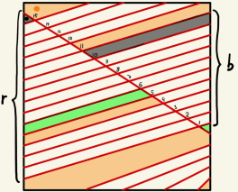
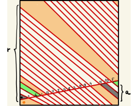
Figure 3. Kawamata Lagrangian $\mathbb{K}_{r,a}$ (here $r=16$, $a=3$, $b=11$)

It has $r-1$ self-intersection points, which we label by elements of $\mathbb{Z}_{r}\setminus\{0\}$.

The proof occupies the rest of this section. We will use a different construction of the Kawamata bundle $F$ from [9], which we are going to recall. Consider the minimal resolution $W^{min}$ of the projective surface $W$. The preimage of the singular point is a chain of rational curves $\Gamma_{1},\ldots,\Gamma_{t}\subset W^{min}$ with self-intersection numbers $-b_{1},\ldots,-b_{t}$ such that $b_{1},\ldots,b_{t}\geq 2$ (see Figure 4.)

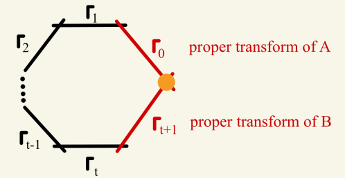
Figure 4. Minimal resolution $W^{min}$ of the projective surface $W$

Remark 2.5.

An explicit model of $W^{min}$ can be constructed as follows: start with a rational elliptic fibration with a $1$-nodal fiber, blow up the node $t+1$ times to create a cycle of $t+2$ projective lines, then blow-up disjoint smooth points on $t$ of the irreducible components to create a chain $\Gamma_{1},\ldots,\Gamma_{t}$ as above. Contracting the chain gives a projective surface $W$ that satisfies Assumptions 1.10 of [24].

Definition 2.6.

There is an exceptional collection on $W^{min}$ of the line bundles

$$L_{t}=\mathcal{O}(-\Gamma_{0}-\Gamma_{1}-\ldots-\Gamma_{t}),\ \ldots,\ L_{1}=\mathcal{O}(-\Gamma_{0}-\Gamma_{1}),\ L_{0}=\mathcal{O}(-\Gamma_{0}).$$ (4)

Lemma 2.7.

Let $E_{t+2}=\Gamma_{0}\cup\ldots\cup\Gamma_{t+1}\subset W^{min}$. Let $L$ be a line bundle on $E_{t+2}$ of multi-degree $(1-\xi,0,0,\ldots,0,1)$, where $\xi=\Gamma_{0}^{2}$. Under mirror symmetry, the mirror Lagrangians $\mathbb{L}_{0},\ldots,\mathbb{L}_{t}\in\mathcal{F}(\mathbb{T}_{t+2})$ of the line bundles $L\otimes L_{0}|_{E_{t+2}},\ldots,L\otimes L_{t}|_{E_{t+2}}$ are illustrated in Figure 5 (for $t=3$). Concretely, each Lagrangian $\mathbb{L}_{i}$ winds $b_{j}-2$ (resp., $b_{j}-1$) times between the punctures $P_{j-1}$ and $P_{j}$ for $j<i$ (resp., $j=i$). We endow these Lagrangians with bounding spin structure, trivial local system and standard grading.

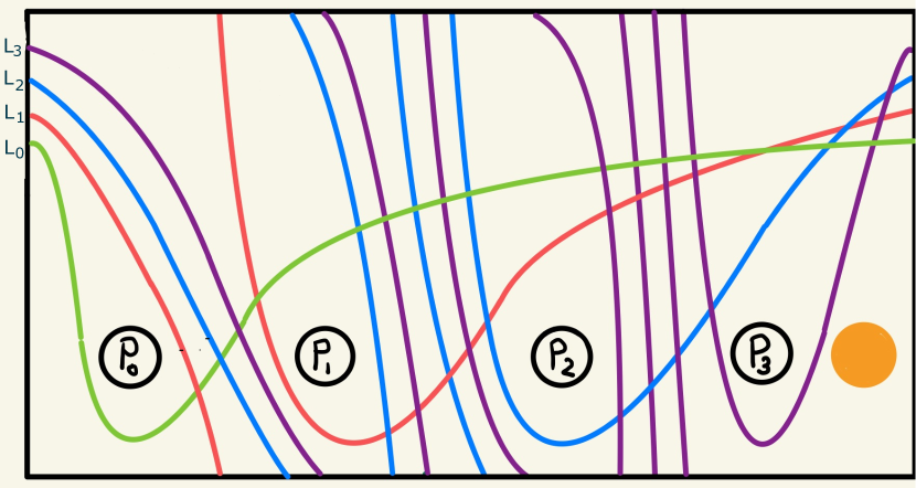
Figure 5. Lagrangians $\mathbb{L}_{0},\ldots,\mathbb{L}_{t+1}\in\mathcal{F}(\mathbb{T}_{t+2})$.

Proof.

The line bundles $L\otimes L_{0}|_{E_{t+2}},\ldots,L\otimes L_{t}|_{E_{t+2}}$ have the following degrees on irreducible components $\Gamma_{0},\ldots,\Gamma_{t+1}$:

$$(L\otimes L_{i})\cdot\Gamma_{j}=\begin{cases}0&\operatorname{if}j\geq i+2\\ -1&\operatorname{if}j=i+1\\ b_{j}-1&\operatorname{if}i=j\geq 1\\ b_{j}-2&\operatorname{if}i>j\geq 1\\ \ 0&\operatorname{if}i>j=0\\ -1&\operatorname{if}i=j=0\\ \end{cases}\qquad\hbox{\rm for}\quad i=0,\ldots,t,\ j=0,\ldots,t+1.$$

We can choose smooth points $q_{i}\in\Gamma_{i}$ for $i=0,\ldots,t+1$ so that

$$L\otimes L_{i}|_{E_{t+2}}=\mathcal{O}(-q_{i+1}+\sum_{j\leq i}a_{ij}q_{j}).$$ (5)

for $i=0,\ldots,t$ and for some integer coefficients $a_{ij}$.

The mirror of the curve $E_{t+2}$ of arithmetic genus $1$ is a torus $\mathbb{T}_{t+2}$ with $t+2$ punctures illustrated in Figure 6 along with the mirror Lagrangians $[\mathcal{O}_{E_{t+2}}]$ and $[\mathcal{O}_{q_{i}}]$ corresponding to $\mathcal{O}_{E_{t+2}}$ and the skyscraper sheaves $\mathcal{O}_{q_{i}}$, where $q_{i}$ for $i=0,\ldots,t+1$ are choices of smooth points on each $\mathbb{P}^{1}$ component. We choose these points so that (5) holds. Line bundles on $E_{t+2}$ of the form $\mathcal{O}(\sum a_{i}q_{i})$ are obtained by twisting $\mathcal{O}_{E_{t+2}}$ by twist functors $T_{\mathcal{O}_{q_{i}}}$ which on the symplectic side are given by Dehn twists around the vertical Lagrangians $[\mathcal{O}_{q_{i}}]$. For example, a line bundle $\mathcal{O}(q_{t+1})$, which restricts to $\mathcal{O}(1)$ in the $(t+1)$-component and to $\mathcal{O}$ on the other components fits in to an exact sequence $0\to\mathcal{O}\to\mathcal{O}(q_{t+1})\to\mathcal{O}_{q_{t+1}}\to 0$.The corresponding Lagrangian $[\mathcal{O}(q_{t+1})]$ is obtained by twisting the Lagrangian $[\mathcal{O}]$ around the Lagrangian $[\mathcal{O}_{q_{t+1}}]$ by a right handed Dehn twist as shown on the right side of Figure 6. We use formula (5) and apply Dehn twists repeatedly to construct Lagrangians $\mathbb{L}_{0},\ldots,\mathbb{L}_{t}$ of the lemma. ∎

Figure 6. Punctured torus $\mathbb{T}_{t+2}$ with oriented Lagrangians corresponding to various perfect sheaves on $E_{t+2}$.

Proof of Theorem 2.4.

By [9] (based on results of [8]), the Kawamata vector bundle on $W$ is isomorphic to the push-forward of a certain vector bundle $F_{0}$ on $W^{min}$, which is the first term in the sequence of vector bundles $F_{0},\ldots,F_{t}$ on $W^{min}$.Concretely, $F_{t}=L_{t}$ and, for $i=0,\ldots,t-1$, the bundle $F_{i}$ is the universal extension of $F_{i+1}$ by $L_{i}$, i.e. we have a short exact sequence

$$0\to{\mathop{\hbox{\rm{Ext}}}}^{1}(F_{i+1},L_{i})^{*}\otimes L_{i}\to F_{i}\to F_{i+1}\to 0.$$ (6)

Lemma 2.8 ([9]).

We have $\dim{\mathop{\hbox{\rm{Ext}}}}^{1}(F_{i+1},L_{i})=\mathop{\hbox{\rm{rk}}}F_{i}-\mathop{\hbox{\rm{rk}}}F_{i+1}$ and

$${\mathop{\hbox{\rm{rk}}}F_{i}\over\mathop{\hbox{\rm{rk}}}F_{i+1}}=b_{i+1}-{1\over b_{i+2}-{1\over\ldots-{1\over b_{t}}}},$$

where $\mathop{\hbox{\rm{rk}}}F_{i}$ and $\mathop{\hbox{\rm{rk}}}F_{i+1}$ are coprime, $-b_{1},\ldots,-b_{t}$ are self-intersections of the exceptional curves in the minimal resolution $W^{min}$ of $W$, and

$${r\over r-a}=b_{1}-{1\over b_{2}-{1\over\ldots-{1\over b_{t}}}}.$$

Let $\mathbb{F}_{i}$ be the Lagrangian in $\mathbb{T}_{t+2}$ corresponding to the vector bundle $F_{i}|_{E_{t+2}}\otimes L$ (here $L$ is a line bundle from Lemma 2.7). We investigate the sequence of Lagrangians $\mathbb{F}_{0},\ldots,\mathbb{F}_{t}$ inductively. Since (4) is an exceptional collection, an argument similar to the proof of Lemma 2.2 shows that

$$\mathop{\hbox{\rm{Ext}}}\nolimits^{j}(F_{i+1},L_{i})\cong\mathop{\hbox{\rm{Ext}}}\nolimits^{j}(F_{i+1}|_{E_{t+2}},L_{i}|_{E_{t+2}})$$

for every $j$. In particular, $F_{i}|_{E_{t+2}}$ is determined inductively by an exact sequence

$$0\to\mathop{\hbox{\rm{Ext}}}\nolimits^{1}(F_{i+1}|_{E_{t+2}},L_{i}|_{E_{t+2}})^{*}\otimes L_{i}|_{E_{t+2}}\to F_{i}|_{E_{t+2}}\to F_{i+1}|_{E_{t+2}}\to 0.$$ (7)

Tensoring (7) with a line bundle $L$ of Lemma 2.7 and applying mirror symmetry, shows that the Lagrangian $\mathbb{F}_{i}$ is determined recursively by the exact triangle ${\mathop{\hbox{\rm{Ext}}}}^{1}(\mathbb{F}_{i+1},\mathbb{L}_{i})^{*}\otimes\mathbb{L}_{i}\to\mathbb{F}_{i}\to\mathbb{F}_{i+1}$ in $\mathcal{F}(\mathbb{T}_{t+2})$.

Lemma 2.9.

The Lagrangian $\mathbb{F}_{i}$ can be constructed as follows: repeat the Lagrangian $\mathbb{L}_{i}$ as many times as the dimension of $\mathop{\hbox{\rm{Ext}}}^{1}(F_{i+1},L_{i})$ (computed in Lemma 2.8). Then perform the surgery illustrated at the top of Figure 7,

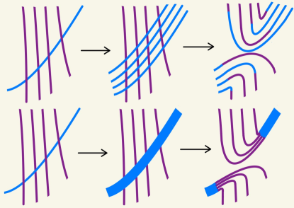
Figure 7. Surgery on Lagrangians

where the Lagrangian $\mathbb{L}_{i}$ is in blue and the Lagrangian $\mathbb{F}_{i+1}$ is in magenta. By aesthetic reasons, instead of repeating the Lagrangian $\mathbb{L}_{i}$, we instead draw a thick “band” of curves as at the bottom of Figure 7.

Proof.

This follows from [1, Lemma 5.4]. ∎

To simplify the analysis, we now restrict to the case $t=3$ but the algorithm is the same for any $t$. We start with $\mathbb{F}_{3}=\mathbb{L}_{3}$, draw $\mathop{\hbox{\rm{rk}}}\mathbb{F}_{2}-\mathop{\hbox{\rm{rk}}}\mathbb{F}_{3}=b_{3}-1$ copies of the “blue” Lagrangian $\mathbb{L}_{2}$ and first construct and then simplify the Lagrangian $\mathbb{F}_{2}$ using Lemma 2.9 as illustrated in Figure 8.

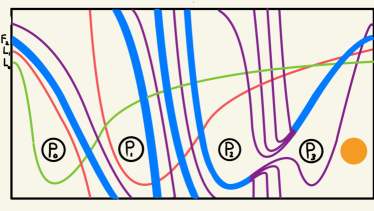
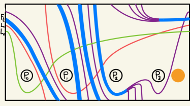
Figure 8. The mirror Lagrangian $\mathbb{F}_{2}$ of the vector bundle $F_{2}$.

Next, we draw $\mathop{\hbox{\rm{rk}}}\mathbb{F}_{1}-\mathop{\hbox{\rm{rk}}}\mathbb{F}_{2}=b_{2}b_{3}-b_{3}-1$ copies of the “red” Lagrangian $\mathbb{L}_{1}$ and construct (and simplify) the Lagrangian $\mathbb{F}_{1}$ illustrated in Figure 9 (left side).

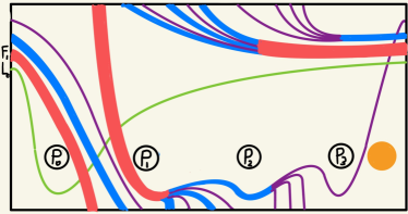
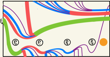
Figure 9. The Lagrangians $\mathbb{F}_{1}$ (left) and $\mathbb{F}_{0}$ (right.)

Finally, we draw $\mathop{\hbox{\rm{rk}}}\mathbb{F}_{0}-\mathop{\hbox{\rm{rk}}}\mathbb{F}_{1}=b_{1}b_{2}b_{3}-b_{2}b_{3}-b_{1}-b_{3}+1$ copies of the “green” Lagrangian $\mathbb{L}_{0}$ and construct (and simplify) the Lagrangian $\mathbb{F}_{0}$ illustrated in Figure 9 (right side).

It remains to observe that the vector bundle $F_{0}|_{E_{t+2}}$ is a pull-back of the Kawamata vector bundle $F|_{E}$. Under mirror symmetry, this means that the Lagrangian $\mathbb{K}_{r,a}$ on the two-punctured torus that corresponds to the Kawamata vector bundle $F|_{E}$ (tensored by $L$) is obtained from the Lagrangian $\mathbb{F}_{0}$ by combining all non-orange punctures into one black puncture. Slightly simplifying Figure 9 shows that this Lagrangian $\mathbb{K}_{r,a}$ is the same as the one from the right side of Figure 3. ∎

The following corollary is straightforward.

Corollary 2.10.

The complement of $\mathbb{K}_{r,a}$ in the torus is the union of rectangular (in other words, four sided) regions, except for one hexagonal region (which contains an orange puncture) and two triangular regions (one of which contains a black puncture).In Figure 10 we draw the region formed by combining the hexagonal and triangular regions, the Gauss word formed by following the Lagrangian until all self-intersection points are counted twice, and the universal cover of the torus with the preimage of $\mathbb{K}_{r,a}$.

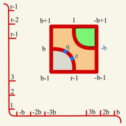
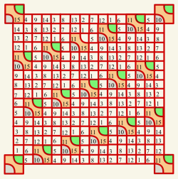
Figure 10. The union of non-rectangular regions, the Gauss word, and the universal cover (for $r=16$, $a=3$, $b=11$.)

3. Deformations of Lagrangians and their endomorphism rings

As in Section 2, let $F_{E}$ be the restriction of the Kawamata vector bundle $F$ to the divisor $E\cong E_{2}$ of the projective algebraic surface $W$ with a cyclic quotient singularity ${1\over r}(1,a)$. In Theorem 3, we found the mirror Lagrangian $\mathbb{K}_{r,a}\in\mathcal{F}(\mathbb{T}_{2})$ of $F_{E}$. We will study the endomorphism algebra $R_{r,a}$ of $\mathbb{K}_{r,a}$ and its deformations.

The motivation comes from the study of flat deformations $(\mathcal{E}\subset\mathcal{W})$ of the pair $(E\subset W)$ over a smooth curve germ $\mathop{\hbox{\rm{Spec}}}A$. Let $t\in A$ be a local parameter.We assume that a general fiber $\mathcal{W}_{t}$ is a smooth projective surface but its anti-canonical divisor $\mathcal{E}_{t}$ has one node. From the divisor $E\cong E_{2}$ of $W$ (see Figure 1), we obtain the divisor $\mathcal{E}_{t}\cong E_{1}$ of $\mathcal{W}_{t}$ by smoothening the black node $P\in E$ but retaining the orange node $Q\in E$.

As explained in [24], the Kawamata vector bundle $F$ on $W$ deforms uniquely to a vector bundle $\mathcal{F}$ on $\mathcal{W}$ and the Kalck–Karmazyn algebra $R_{r,a}={\mathop{\hbox{\rm{End}}}}(F)$ deforms to a $A$-algebra $\mathcal{R}={\mathop{\hbox{\rm{End}}}}(\mathcal{F})$, which is a free $A$-module of rank $r$. The $A$-algebra $\mathcal{R}$ depends on the deformation of $(E\subset W)$. Concretely, the versal deformation space ${\mathop{\hbox{\rm{Def}}}}_{(E\subset W)}$ has several irreducible components, which are all smooth and classified in [14] (Kollár–Shepherd-Barron correspondence). If $(\mathcal{E}\subset\mathcal{W})$ is a general deformation within a fixed irreducible component of ${\mathop{\hbox{\rm{Def}}}}_{(E\subset W)}$, then the general fiber $\mathcal{R}_{t}$ of the family of algebras $\mathcal{R}$ is a hereditary algebra by [24] (equivalently, $\mathcal{R}_{t}$ is Morita-equivalent to a path algebra of a quiver without relations).

We would like to compute the $A$-algebra $\mathcal{R}$ explicitly. Our idea is to use the following formula, which can be proved in the same way as Lemma 2.2:

$$\mathcal{R}={\mathop{\hbox{\rm{End}}}}(\mathcal{F})\cong{\mathop{\hbox{\rm{End}}}}(\mathcal{F}|_{\mathcal{E}}).$$ (8)

In this section we focus on computing the closed subscheme ${\mathop{\hbox{\rm{Def}}}}^{0}_{F_{E}/\mathcal{E}}\subset{\mathop{\hbox{\rm{Def}}}}_{F_{E}/\mathcal{E}}$ (see Definition 1.7) and the flat family of finite-dimensional algebras ${\mathop{\hbox{\rm{End}}}}(\mathcal{V}_{p})$ over it that provides a deformation of the Kalck–Karmazyn algebra $R_{r,a}={\mathop{\hbox{\rm{End}}}}(F_{E})$.

Remark 3.1.

A minor nuisance is that an algebraic surface $\mathcal{E}$ can have a singularity at the node $P$ of the special fiber $E$ of type $A_{\ell-1}$, $\ell\geq 1$. We have a finite base change cartesian diagram

$$\begin{CD}\mathcal{E}@>{}>{}>\mathscr{E}\\ @V{}V{}V@V{}V{}V\\ \mathop{\hbox{\rm{Spec}}}A@>{}>{}>\mathop{\hbox{\rm{Spec}}}B\\ \end{CD}$$ (9)

where $B\subset A$ is a subring with local parameter $s=t^{\ell}$ and $\mathscr{E}$ is a versal deformation of $P\in E$ (equisingular at $Q\in E$.) The total space of $\mathscr{E}$ is smooth at $P$. Since ${\mathop{\hbox{\rm{Def}}}}^{0}_{F_{E}/\mathcal{E}}\subset{\mathop{\hbox{\rm{Def}}}}_{F_{E}/\mathcal{E}}$ is a base change of ${\mathop{\hbox{\rm{Def}}}}^{0}_{F_{E}/\mathscr{E}}\subset{\mathop{\hbox{\rm{Def}}}}_{F_{E}/\mathscr{E}}$, in this section we will do all calculations on $\mathscr{E}$ and worry about the finite base change later.

Remark 3.2.

Note that irreducible components of ${\mathop{\hbox{\rm{Def}}}}^{0}_{F_{E}/\mathscr{E}}$ are not necessarily smooth over $\mathop{\hbox{\rm{Spec}}}B$. So $1$-parameter deformations of $R_{r,a}$ contained in these components are not necessarily parametrized by $s\in B$ but may require a finite base change (such as $t\in A$).

In the remainder of this section, we will describe the closed subscheme ${\mathop{\hbox{\rm{Def}}}}^{0}_{F_{E}/\mathscr{E}}$ and the family of algebras ${\mathop{\hbox{\rm{End}}}}(\mathcal{V}_{p})$ over it using homological mirror symmetry for the family of genus one curves $\mathscr{E}$. The answer is given in Corollary 3.5.

Recall that that the mirror of $F_{E}$ is an immersed oriented Lagrangian $\mathbb{K}_{r,a}$ on a symplectic torus $\mathbb{T}_{2}$ with two punctures (orange and black) equipped with brane data (bounding spin structure, trivial local system, and standard grading).In the previous section, we worked with the exact Fukaya category of $\mathbb{T}_{2}$ as defined in [23], which provides a mirror for $E_{2}$. In this section, we re-interpret the black puncture as a divisor $\{s\}\subset\mathbb{T}_{1}$ on a one-punctured torus. The computations will take place in the relative exact Fukaya category $\mathcal{F}(\mathbb{T}_{1},\{s\})$, which provides a mirror for the family of genus $1$ curves $\mathscr{E}\to\mathop{\hbox{\rm{Spec}}}B$. Indeed, [16] establishes mirror symmetry for the Tate family of curves $T_{2}\to\mathrm{Spec}\,\mathbb{Z}[[t_{1},t_{2}]]$, which is the total space of the versal formal deformations of the special fiber $E_{2}$ (see [16, Section 2]). The main result [16, Theorem A] establishes a quasi-equivalence $\mathcal{F}(\mathbb{T},\{s,o\})\simeq\mathrm{Perf}\,T_{2}$ over $\mathbb{Z}[[t_{1},t_{2}]]$, where the left-hand-side is the split-closed derived Fukaya category of the compact torus $\mathbb{T}$ relative to compactification divisor given by 2 points $\{s,o\}$. Note that $\mathbb{T}\setminus\{s,o\}=\mathbb{T}_{2}$. In the relative Fukaya category $t_{1}$ (resp. $t_{2}$) is a formal parameter keeping track of the intersection number of holomorphic polygons with $s$ (resp. $o$). The family of genus 1 curves $\mathscr{E}\to\mathop{\hbox{\rm{Spec}}}B$ corresponds to the subfamily $(t_{2}=0)$, where the curve $E_{2}$ deforms to a curve $E_{1}$ by smoothing a black node $P$ and retaining an orange node $Q$ in Figure 1. The techniques used in the proof of Theorem [16, Theorem A] apply directly in this case to give the quasi-equivalence over $B$,

$$\mathcal{F}(\mathbb{T}_{1},\{s\})\simeq\mathrm{Perf}\,\mathscr{E}.$$ (10)

Here $\mathbb{T}_{1}$ is once-punctured torus, $D=\{s\}$ (formerly known as a black puncture) is a divisor with respect to which we study the relative Fukaya category and $\mathscr{E}\to\mathop{\hbox{\rm{Spec}}}B$ is the family of nodal curves where the special fiber is the $E_{2}$ and general fiber is $E_{1}$, the nodal rational curve. The $A_{\infty}$-category $\mathcal{F}(\mathbb{T}_{1},\{s\})$ is $B$-linear. The $A_{\infty}$-operations are given by counting holomorphic polygons with boundaries on Lagrangians, but the contribution of each polygon $u$ comes with a weight $s^{\mathrm{mult}(u,\{s\})}$. (See [16] for more background on relative Fukaya categories.)

We can view the Kawamata Lagrangian $\mathbb{K}:=\mathbb{K}_{r,a}$ as an object of $\mathcal{F}(\mathbb{T}_{1},\{s\})$, which is a mirror of some deformation of the Kawamata vector bundle $F_{E}$ to a vector bundle on $\mathscr{E}$. We start by computing the $A_{\infty}$-algebra $(\mathscr{A}_{\mathbb{K}},\{\mathfrak{m}_{i}\}_{i\geq 1})$ of endomorphisms of $\mathbb{K}$ as an object in $\mathcal{F}(\mathbb{T}_{1},\{s\})$. We follow the sign conventions as given in [23, Ch. 1]. Recall that an $A_{\infty}$-algebra $\mathscr{A}$ over a commutative ring $B$ is a $\mathbb{Z}$-graded $B$-module with a collection of $B$-linear maps $\mathfrak{m}_{i}:\mathscr{A}^{\otimes i}\to\mathscr{A}[2-i]$ for $i\geq 1$, where the notation $\mathscr{A}[2-i]$ means that $\mathfrak{m}_{i}$ lowers the degree by $i-2$. These maps are required to satisfy the $A_{\infty}$-relations:

$$\sum_{j,k}(-1)^{|a_{1}|+\ldots+|a_{j}|-j}\mathfrak{m}_{i-k+1}(a_{i},\ldots,a_{j+k+1},\mathfrak{m}_{k}(a_{j+k},\ldots,a_{j+1}),a_{j},\ldots,a_{1})=0.$$

The cohomology with respect to $\mathfrak{m}_{1}$ is an associative algebra with the product:

$$a_{2}a_{1}=(-1)^{|a_{1}|}\mathfrak{m}_{2}(a_{2},a_{1}).$$

The underlying complex of $(\mathscr{A}_{\mathbb{K}},\{\mathfrak{m}_{i}\}_{i\geq 1})$ is the Floer cochain complex given as a $B$-module by

$$CF(\mathbb{K},\mathbb{K})=\mathrm{hom}^{0}(\mathbb{K},\mathbb{K})\oplus\mathrm{hom}^{1}(\mathbb{K},\mathbb{K}),\quad\hbox{\rm where}$$

$$\mathrm{hom}^{0}(\mathbb{K},\mathbb{K})=Bw_{0}\oplus\bigoplus_{i=1}^{r-1}Bw_{i}\quad\hbox{\rm and}\quad\mathrm{hom}^{1}(\mathbb{K},\mathbb{K})=B\bar{w}_{0}\oplus\bigoplus_{i=1}^{r-1}B\bar{w}_{i}.$$

Definition 3.3.

For $i\neq 0$, we associate a pair of generators ${w_{i},\bar{w}_{i}}$ with each self-intersection point of the Lagrangian  $\mathbb{K}$. The generators $e=w_{0}$ and $q=\bar{w}_{0}$, placed as illustrated in Figure 13, correspond to the minimum and the maximum of a Morse function chosen on the domain of the immersion of the Lagrangian.

Theorem 3.4.

The $A_{\infty}$-algebra $(\mathscr{A}_{\mathbb{K}_{r,a}},\{\mathfrak{m}_{i}\}_{i\geq 1})$ has the following products:

1. For $i=0,\ldots,r-1$,

   $$\mathfrak{m}_{2}(w_{i},w_{0}) =w_{i}=\mathfrak{m}_{2}(w_{0},w_{i})$$

   $$\mathfrak{m}_{2}(\bar{w}_{i},w_{0}) =\bar{w}_{i}=-\mathfrak{m}_{2}(w_{0},\bar{w}_{i})$$

   $$\mathfrak{m}_{2}(\bar{w}_{i},w_{i}) =\bar{w}_{0}=-\mathfrak{m}_{2}(w_{i},\bar{w}_{i})$$

2. For each $i\neq 0$,

   $$\mathfrak{m}_{3}(\bar{w}_{i},w_{i},\bar{w}_{i}) =-\bar{w}_{i}$$

   $$\mathfrak{m}_{3}(\bar{w}_{i},w_{i},\bar{w}_{0}) =-\bar{w}_{0}$$

   $$\mathfrak{m}_{3}(w_{i},\bar{w}_{i},\bar{w}_{0}) =\bar{w}_{0}$$

3. For each sub-interval $(x,y)$ of the Gauss word (see Figure 10)

   $$w_{r-1},w_{r-2},\ldots,w_{1},w_{-b},w_{-2b},\ldots,w_{-(r-1)b},$$

   $$\mathfrak{m}_{3}(y,\bar{x},x)=y,\ \mathfrak{m}_{3}(\bar{x},x,\bar{y})=-\bar{y}\quad x y \{-b,-2b,\ldots,-(r-1)b\}$$ if both and are in ,

   $$\mathfrak{m}_{3}(x,\bar{x},\bar{y})=\bar{y},\ \mathfrak{m}_{3}(y,x,\bar{x})=-y\quad x\in\{r-1,\ldots,1\} y\in\{-b,\ldots,-(r-1)b\}$$ if and ,

   $$\mathfrak{m}_{3}(\bar{y},x,\bar{x})=-\bar{y},\ \mathfrak{m}_{3}(x,\bar{x},y)=-y\quad x y \{r-1,r-2,\ldots,1\}$$ if both and are in .

4. Products that correspond to ‘visible’ polygons are described in Figure 11.

   

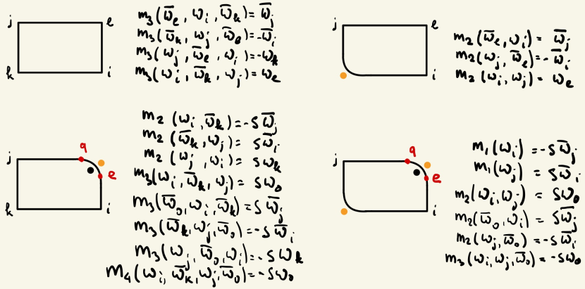
   Figure 11. Contributions to $\mathscr{A}_{\mathbb{K}_{r,a}}$ from visible holomorphic polygons

Proof.

Let $\mathbb{K}:=\mathbb{K}_{r,a}$. The $A_{\infty}$ structure of $\mathscr{A}_{\mathbb{K}}$ is defined via counts of holomorphic polygons with boundary on $\mathbb{K}$. We stick to the conventions laid out in [22, Section 7]. When working with Fukaya categories of surfaces, the holomorphic curve contributions come in two flavors. There are “visible” immersed polygons with boundary on the Lagrangians, and “virtual” polygons which only become visible after successive perturbations of the Lagrangians. Before perturbing, the corresponding moduli spaces are in general not regular around constant maps for polygons with more than three edges (see [18] for an illustration), hence to count these contributions correctly one has to use virtual fundamental chains or else perturb. A concrete way to deal with this issue in the case of surfaces is by taking successive push-offs of the Lagrangian using a small Hamiltonian perturbation. Fortunately, in this paper, other than the bigons and triangles that contribute to the differential $\mathfrak{m}_{1}$ and the product $\mathfrak{m}_{2}$ for which regularity can be arranged (even before perturbing, see [22, Section 7]), we will only deal with holomorphic rectangles to compute the contributions to $\mathfrak{m}_{3}$ and the perturbations by push-offs still remain manageable. Taking only the virtual contributions into account, one gets a model for the Fukaya category of the Weinstein neighborhood of the immersed Lagrangian (a plumbing) which can be described with an $A_{\infty}$-algebra with $\mathfrak{m}_{i}\neq 0$ only for $i=2,3$. We call this algebra a hidden $A_{\infty}$ algebra $\mathscr{A}_{0}$. The contributions (1), (2), (3) to the $A_{\infty}$ algebra $\mathscr{A}_{\mathbb{K}}$ come from this hidden algebra.

Figure 12. Kawamata Lagrangian of ${1\over 2}(1,1)$.

We will only compute these contributions in the simplest example of ${1\over 2}(1,1)$, since the general case is similar. The Kawamata Lagrangian is illustrated in Figure 12, where we denote $w_{1}$ by  $x$. We have

$$\mathrm{hom}^{0}(L,L)=\mathbb{Z}e\oplus\mathbb{Z}x\quad\hbox{\rm and}\quad\mathrm{hom}^{1}(L,L)=\mathbb{Z}q\oplus\mathbb{Z}\bar{x}.$$

Following the statement of Theorem 3.4, in addition to $m_{2}$ products from (1), we need to find three $m_{3}$ products from (2) and two $m_{3}$ products from (3) (the Gauss word is $\{1,1\}$ and only the second case of (3) is present). These triple products are

$$\mathfrak{m}_{3}(x,x,\bar{x}) =-x$$

$$\mathfrak{m}_{3}(x,\bar{x},\bar{x}) =\bar{x}=-\mathfrak{m}_{3}(\bar{x},x,\bar{x})$$

$$\mathfrak{m}_{3}(x,\bar{x},q) =q=-\mathfrak{m}_{3}(\bar{x},x,q)$$

They can be checked by perturbing the Lagrangian by taking three push-offs. The next figure shows the rectangle that gives the triple product $\mathfrak{m}_{3}(x,x,\bar{x})=-x$. The reader is invited to find rectangles that give other triple products listed above.

The contributions via perturbation are computed in the following manner. Let $L$, ${\color[rgb]{0,0,1}L^{\prime}}$, ${\color[rgb]{1,0,0}L^{\prime\prime}}$ and ${\color[rgb]{0.0,0.5,0.0}L^{\prime\prime\prime}}$ are the original Lagrangian and its push-offs. Then, treating these Lagrangians as separate, we compute the triangle that contributes to the product

$$\mathfrak{m}_{3}:CF({\color[rgb]{1,0,0}L^{\prime\prime}},{\color[rgb]{0.0,0.5,0.0}L^{\prime\prime\prime}})\otimes CF({\color[rgb]{0,0,1}L^{\prime}},{\color[rgb]{1,0,0}L^{\prime\prime}})\otimes CF(L,{\color[rgb]{0,0,1}L^{\prime}})\to CF(L,{\color[rgb]{0.0,0.5,0.0}L^{\prime\prime\prime}})$$

This means looking for rectangles (in the case of $\mathfrak{m}_{3}$) whose boundary traces the Lagrangians $L$, ${\color[rgb]{0,0,1}L^{\prime}}$, ${\color[rgb]{1,0,0}L^{\prime\prime}}$ and ${\color[rgb]{0.0,0.5,0.0}L^{\prime\prime\prime}}$ in the counter-clockwise order. The corner between $L,{\color[rgb]{0.0,0.5,0.0}L^{\prime\prime\prime}}$ is treated as an output and all the others are input. Once we orient our Lagrangians (which we always do in the way indicated), an intersection point $p\in CF(L,K)$ corresponds to a degree 0 generator if the intersection number $L\cdot K=-1$ and a degree 1 generator if the intersection number $L\cdot K=+1$. The sign contribution of a polygon is determined according to whether the orientation of the Lagrangians in its boundary matches with the counter-clockwise orientation of the boundary of the polygon, see [22, Section 7] for a detailed explanation. Finally, to get the product defined on $CF(L,L)$, we identify $CF(L,L)$ with $CF(L,{\color[rgb]{0,0,1}L^{\prime}})$, $CF({\color[rgb]{0,0,1}L^{\prime}},{\color[rgb]{1,0,0}L^{\prime\prime}})$, $CF({\color[rgb]{1,0,0}L^{\prime\prime}},{\color[rgb]{0.0,0.5,0.0}L^{\prime\prime\prime}})$ and $CF(L,{\color[rgb]{0.0,0.5,0.0}L^{\prime\prime\prime}})$. In general, these identifications might be non-trivial to compute but in the case of surfaces the are straightforward.

Finally, we analyze contributions to $\mathscr{A}_{\mathbb{K}}$ given by equations Theorem 3.4 (4). They come from the visible holomorphic polygons, for which the corresponding moduli spaces are regular. We illustrate some visible polygons in Figure 13.

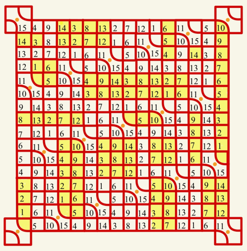
Figure 13. Some visible holomorphic polygons

We can view these contributions as providing an $A_{\infty}$ deformation of the hidden $A_{\infty}$-algebra $\mathscr{A}_{0}$ to $\mathscr{A}_{\mathbb{K}}$. A special feature of our Lagrangian $\mathbb{K}$ is its grid-like structure, illustrated in Figure 13. It implies that all visible polygons with boundary on $\mathbb{K}$ that do not contain the orange puncture (but may contain the black puncture) are either rectangles or degenerations of rectangles (bigons or triangles), where the missing vertices of a rectangle correspond to the curved sections of the Kawamata Lagrangian passing close to the orange puncture. These polygons are given in Figure 11. In the ${1\over 2}(1,1)$ example, only the bigon from the bottom right corner of Figure 11 shows up. Since $i=j=1$ in this case, the contributions to $m_{1}$ cancel each other out, leaving the products

$$\mathfrak{m}_{2}(x,x)=s\cdot e=-\mathfrak{m}_{3}(x,x,q)\quad\hbox{\rm and}\quad\mathfrak{m}_{2}(q,x)=s\cdot\bar{x}=-\mathfrak{m}_{2}(x,q)$$

Computing these products for general $(r,a)$ is a routine calculation providing several cases summarized in Figure 11. ∎

The Kawamata Lagrangian $\mathbb{K}=\mathbb{K}_{r,a}$ is the mirror of one possible deformation of the vector bundle $F_{E}$ to the family of genus $1$ curves $\mathscr{E}$. To compute the mirrors of all possible deformations, we use the formalism of bounding cochains.

Let $\mathfrak{b}\in CF^{1}(\mathbb{K},\mathbb{K})$. By Fukaya–Oh–Ohta–Ono [5], the new products

$$\mathfrak{m}^{\mathfrak{b}}_{i}(x_{i},x_{i-1},\ldots,x_{1})=\sum_{j\geq i}\mathfrak{m}_{j}(\mathfrak{b},\ldots,\mathfrak{b},x_{i},\mathfrak{b},\ldots,\mathfrak{b},x_{i-1},\mathfrak{b},\ldots,\ldots,\mathfrak{b},x_{1},\mathfrak{b},\ldots,\mathfrak{b})$$

give a deformed $A_{\infty}$-algebra if the bounding cochain $\mathfrak{b}$ satisfies the Maurer–Cartan equation

$$\mathfrak{m}_{1}(\mathfrak{b})+\mathfrak{m}_{2}(\mathfrak{b},\mathfrak{b})+\ldots=0.$$

In our case, this equation is automatic because $CF(\mathbb{K},\mathbb{K})$ has no generators in degree 2. Thus, we have the following immediate corollary of Theorem 3.4.

Corollary 3.5.

Fix a bounding cochain $\mathfrak{b}=\sum\limits_{i\in\mathbb{Z}_{r}}t_{i}\bar{w}_{i}\in CF^{1}(\mathbb{K},\mathbb{K})$. Contributions to the differentials $dw_{i}=m_{1}^{\mathfrak{b}}(w_{i})$ and to the products $w_{i}w_{j}=m_{2}^{\mathfrak{b}}(w_{i},w_{j})$ in the relative Fukaya category of $\mathcal{F}(\mathbb{T}_{1},\{s\})$ are given in Figure 14, where $s$ needs to be replaced by $s(1-t_{0})$ (in practice, we will assume that $t_{0}=0$, so this doesn’t matter.)

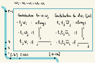
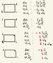
Figure 14. Contributions from virtual (left) and visible (right) polygons

Write $dw_{i}=\sum m_{ij}\bar{w}_{j}$ for $i,j=1,\ldots,r-1$. The matrix $\mathfrak{D}=(m_{ij})$ is skew-symmetric. The subscheme ${\mathop{\hbox{\rm{Def}}}}^{0}_{F_{E}/\mathscr{E}}\subset{\mathop{\hbox{\rm{Def}}}}_{F_{E}/\mathscr{E}}$ of Definition 1.7 is cut out by the ideal in $B[t_{0},\ldots,t_{r-1}]$ generated by the matrix entries of $\mathfrak{D}$. Over this subscheme,

$$\mathcal{R}=\mathcal{R}_{\mathfrak{b}}=(\mathrm{hom}^{0}(\mathbb{K},\mathbb{K}),\mathfrak{m}_{2}^{\mathfrak{b}}).$$

gives a flat deformation of the Kalck-Karmazyn algebra $R={\mathop{\hbox{\rm{End}}}}(F_{E})\cong{\mathop{\hbox{\rm{End}}}}(\mathbb{K})$.

Corollary 3.6.

The Kalck–Karmazyn algebra $R_{r,a}$ has multiplication given by (3).One can also write a closed expression for this product. For every $i\in\mathbb{Z}_{r}$, we define $[i]\in\mathbb{Z}$ such that $0\leq[i]<r$ and $i\equiv[i]\mod r$. We define a function $m(j)=\min\limits_{k=1,\ldots,[-aj]}[kb]$ for $j\in\mathbb{Z}_{r}^{*}$ and set $m(0)=r$. Then $R_{r,a}$ has basis $w_{i}$ for $i\in\mathbb{Z}_{r}$ and product

$$w_{j}w_{i}=\begin{cases}w_{j+i}&\hbox{\rm if $m(j)>[i]$}\cr 0&\hbox{\rm otherwise.}\end{cases}$$ (11)

Proof.

When $s=t_{i}=0$ for all $i$, all differentials in Corollary 3.5 trivially vanish and the only contributions to the products $w_{i}w_{j}$ come from visible triangles (see the second row on the right side of Figure 14.) But visible triangles precisely correspond to rectangles in the first quadrant with vertices

$$\begin{matrix}(0,[i])&\dots&([-aj],[i])\cr\vdots&&\vdots\cr(0,0)&\dots&([-aj],0)\cr\end{matrix}$$

does not contain any orange dots except for $(0,0)$. This condition, appearing in (3), is also equivalent to the inequality $m(j)>[i]$. ∎

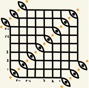
Figure 15. Kawamata Lagrangian for ${1\over r}(1,1)$

In the remainder of this section, we will apply Corollary 3.5 in some examples, starting with the Kawamata Lagrangian that corresponds to the cone over a rational normal curve (cyclic quotient singularity ${1\over r}(1,1)$.)

Since $a=b=1$, the Gauss word is $\{r-1,r-2,\ldots,2,1,r-1,r-2,\ldots,2,1\}$.The Lagrangian is illustrated in Figure 15, c.f. Example 1.5. Take a bounding cochain $\mathfrak{b}=\sum\limits_{i\in\mathbb{Z}_{r}^{*}}t_{i}\bar{w}_{i}$. The hidden algebra $\mathscr{A}_{0}$ gives contributions

to $$dw_{i} t_{i}t_{j}\bar{w}_{j} i<j -t_{i}t_{j}\bar{w}_{j} i>j$$:  if and if

to $$w_{i}w_{j} 0 i<j -t_{j}w_{i}-t_{i}w_{j} i>j -t_{i}w_{i} i=j$$:  if , if and if .

There are two types of visible polygons (the top and the bottom row on the right of Figure 14). The first type is given by $1\leq i<k<j\leq r-1$ (and then $l=i+j-k$). The contributions are

to $$dw_{i} t_{k}t_{l}\bar{w}_{j} dw_{j} -t_{k}t_{l}\bar{w}_{i} w_{i}w_{j} t_{k}w_{l} w_{j}w_{i} -t_{l}w_{k}$$: ; to : ; to : ;  and to : .

Finally, there is only one polygon (=bigon) of the second type, contributing

to $$dw_{r-1} -s\bar{w}_{1} dw_{1} s\bar{w}_{r-1} w_{r-1}w_{1} sw_{0}$$: ; to : ; to : .

Corollary 3.7.

For the singularity ${1\over r}(1,1)$, the skew-symmetric matrix $\mathfrak{D}$ of Corollary 3.5 has entries (for $i<j$) given by

$$m_{ij}=\sum_{k=i}^{j-1}t_{k}t_{i+j-k}$$

except that $m_{1,r-1}$ (if $r>2$) has an additional term $s$.

Legtus analyze the vanishing locus of the matrix $\mathfrak{D}$. There are a few cases depending on $r$.

Example 3.8 ($r=2$).

In this case $\mathfrak{D}=0$, i.e. there are no obstructions to deformations of the Kalck–Karmazyn algebra $R$ over $k[t_{1},s]$. The multiplication is given by $w_{1}^{2}=-t_{1}w_{1}+s$. So the deformation of the Kalck–Karmazyn algebra $R=k[w_{1}]/(w_{1}^{2})$ is given by $k[w_{1}]/(w_{1}^{2}+t_{1}w_{1}-s)$.

Example 3.9 ($r\geq 3$, first component).

One of the solutions of the matrix equation $\mathfrak{D}=0$ is to take $t_{2}=t_{3}=\ldots=t_{r-2}=0$, $s=-t_{1}t_{r-1}$. This is clearly the only possibility if $r=3$. We also claim that this is the only possibility when $r\geq 5$ (although in this case the ideal generated by entries of $\mathfrak{D}$ is not reduced). Indeed, the entries right above the diagonal are $t_{1}t_{2},\ldots,t_{r-2}t_{r-1}$, so some of the variables have to vanish. On the other hand, the entries of the form $m_{i,i+2}$ are $t_{i}t_{i+2}+t_{i+1}^{2}$. So if $t_{i}$ (or $t_{i+2}$) vanishes, then so does $t_{i+1}$. This forces $t_{2}=t_{3}=\ldots=t_{r-2}=0$.

Over $k[t_{1},t_{r-1},s]/(t_{1}t_{r-1}+s)\cong k[t_{1},t_{r-1}]$, the deformed algebra is given by

$$k\langle w_{1},\ldots,w_{r-1},t_{1},t_{r-1}\rangle/\left\langle\begin{aligned} &w_{1}^{2}+t_{1}w_{1},w_{2}^{2},w_{3}^{2},\ldots,w_{r-2}^{2},w_{r-1}^{2}+t_{r-1}w_{r-1}\\ &w_{i}w_{j}\text{ for }i<j,w_{i}w_{j}\text{ for }r-1>i>j>1\\ &w_{i}w_{1}+t_{1}w_{i},w_{r-1}w_{i}+t_{r-1}w_{i}\text{ for }1<i<r-1\\ &w_{r-1}w_{1}+t_{r-1}w_{1}+t_{1}w_{r-1}+t_{1}t_{r-1}\end{aligned}\right\rangle$$

Generically (when $t_{1},t_{r-1}\neq 0$), this gives a deformation of the Kalck-Karmazyn algebra $R_{r,1}=k\langle w_{1},\ldots,w_{r-1}\rangle/(w_{1},\ldots,w_{r-1})^{2}$ to the path algebra of the $(r-2)$-Kronecker quiver via the isomorphism $w_{1}\to a_{1}-t_{1}e_{1},w_{2}\to a_{2},\ldots,w_{r-2}\to a_{r-2},w_{r-1}\to-t_{r-1}e_{2}$.

Example 3.10 ($r=4$, second component).

If $r=4$, there is another possibility for vanishing of the matrix $\mathfrak{D}$, namely $t_{1}=t_{3}=s+t_{2}^{2}=0$. This gives a deformation of the Kalck–Karmazyn algebra $R_{4,1}=k\langle w_{1},w_{2},w_{3}\rangle/(w_{1},w_{2},w_{3})^{2}$ over $k[t_{2},s]/(s+t_{2}^{2})\cong k[t_{2}]$ to the algebra

$$k[t_{2}]\langle w_{1},w_{2},w_{3}\rangle/\left\langle\begin{aligned} &w_{1}w_{2},w_{2}w_{3},w_{1}^{2},w_{3}^{2},w_{2}^{2}+t_{2}w_{2},\\ &w_{1}w_{3}-t_{2}w_{2},w_{3}w_{1}-t_{2}w_{2}+t_{2}^{2},\\ &w_{3}w_{2}+t_{2}w_{3},w_{2}w_{1}+t_{2}w_{1}\end{aligned}\right\rangle$$

For $t_{2}\neq 0$, this algebra is isomorphic to a $2\times 2$ matrix algebra ${\mathop{\hbox{\rm{Mat}}}}_{2}(k)$.

In accordance with Conjecture 1.9, we see that. at least in the case of ${1\over r}(1,1)$, all deformations of the Kalck–Karamazyn algebra $R={\mathop{\hbox{\rm{End}}}}(F_{E})$ over ${\mathop{\hbox{\rm{Def}}}}^{0}_{F_{E}/\mathscr{E}}$ are induced by deformations of the algebraic surface $W$. According to [21], the versal deformation space of $W$ is irreducible for $r\neq 4$ (although non-reduced for $r>4$) and corresponds to Artin deformations of $W$ (deformations induced by a deformation of the resolution of singularities of $W$), while for $r=4$ there is an additional component that corresponds to $\mathbb{Q}$-Gorenstein deformations. According to [24], general Artin deformations of $W$ give deformations of the Kalck–Karamazyn algebra to the path algebra of the Kronecker quiver, while $\mathbb{Q}$-Gorenstein deformations lead to deformations to ${\mathop{\hbox{\rm{Mat}}}}_{2}(k)$. So Example 3.10 gives an explicit presentation for this deformation. In the next section, we will generalize this calculation to arbitrary $\mathbb{Q}$-Gorenstein deformations of Wahl singularities.

Example 3.11.

We wrote a computer code [19] implementation of Corollary 3.5. For example, let $r=15$ and $a=4$. This is the first case when the versal deformation space ${\mathop{\hbox{\rm{Def}}}}_{(E\subset W)}$ of a cyclic quotient singularity has three irreducible components, as can be verified by the computer program [26]. In accordance with Conjecture 1.9, ${\mathop{\hbox{\rm{Def}}}}^{0}_{F_{E}/\mathscr{E}}$ also has three irreducible components given by the ideals

$I_{1}=({t}_{13},{t}_{12},{t}_{11},{t}_{10},{t}_{9},{t}_{6},{t}_{5},{t}_{4},{t}_{3},{t}_{2},{t}_{1}{t}_{14}+s,{t}_{7}^{2}-{t}_{14},{t}_{1}{t}_{7}-{t}_{8})$,

$I_{2}=({t}_{13},{t}_{10},{t}_{9},{t}_{8},{t}_{7},{t}_{6},{t}_{5},{t}_{2},{t}_{1}{t}_{14}+s,{t}_{3}{t}_{11}-{t}_{14},{t}_{1}{t}_{11}-{t}_{12},{t}_{1}{t}_{3}-{t}_{4})$,

$I_{3}=({t}_{14},{t}_{12},{t}_{10},{t}_{9},{t}_{8},{t}_{7},{t}_{6},{t}_{5},{t}_{3},{t}_{1},{t}_{2}{t}_{13}+s,{t}_{2}{t}_{11}-{t}_{13},{t}_{2}^{2}-{t}_{4})$.

Example 3.12.

Another singularity with $3$ irreducible components is ${1\over 19}(1,7)$, which was analyzed in [14]. ${\mathop{\hbox{\rm{Def}}}}^{0}_{F_{E}/\mathscr{E}}$ has $3$ irreducible components given by the ideals

$I_{1}=({t}_{4},{t}_{15},{t}_{6},{t}_{13},{t}_{16},{t}_{3},{t}_{1},{t}_{18},{t}_{8},{t}_{11},{t}_{5}{t}_{7}-{t}_{12},-{t}_{7}^{2}+{t}_{14},{t}_{7}{t}_{12}+s,$

${t}_{2}{t}_{5}-{t}_{7},-{t}_{5}{t}_{12}+{t}_{17},-{t}_{2}{t}_{7}+{t}_{9},-{t}_{5}^{2}+{t}_{10})$

$I_{2}=({t}_{4},{t}_{15},{t}_{7},{t}_{12},{t}_{16},{t}_{3},{t}_{2},{t}_{17},{t}_{1}{t}_{13}-{t}_{14},{t}_{1}{t}_{5}-{t}_{6},-{t}_{5}{t}_{13}+{t}_{18},$

${t}_{6}{t}_{13}+s,{t}_{5}{t}_{8}-{t}_{13},-{t}_{5}{t}_{6}+{t}_{11},-{t}_{1}{t}_{8}+{t}_{9},-{t}_{5}^{2}+{t}_{10})$

$I_{3}=({t}_{4},{t}_{15},{t}_{7},{t}_{12},{t}_{6},{t}_{13},{t}_{5},{t}_{14},{t}_{3}{t}_{16}+s,{t}_{2}{t}_{16}-{t}_{18},{t}_{1}{t}_{2}-{t}_{3},$

$-{t}_{3}{t}_{8}+{t}_{11},-{t}_{1}{t}_{16}+{t}_{17},-{t}_{1}{t}_{8}+{t}_{9},-{t}_{2}{t}_{8}+{t}_{10})$.

4. $\mathbb{Q}$-Gorenstein deformation of the Kalck–Karmazyn algebra

We fix coprime integers $0<q<n$. A cyclic quotient singularity ${1\over n^{2}}(1,nq-1)$ is called a Wahl singularity. It can also be described as $(xy=z^{n})\subset{1\over n}(1,-1,q)$. A special feature of the Wahl singularity is that it admits a $1$-dimensional versal $\mathbb{Q}$-Gorenstein deformation space, namely

$$(xy=z^{n}+t)\subset{1\over n}(1,-1,q)\times\mathbb{A}^{1}_{t}.$$ (12)

We compactify the Wahl singularity to a projective surface $W$ as in Section 2 and let $\mathcal{W}$ be the corresponding projective $\mathbb{Q}$-Gorenstein deformation. After a finite base change, the total space of the deformation carries a torsion-free sheaf $\mathcal{H}$ introduced by Hacking [6] (we use a version from [13]) such that its restriction to a general fiber $\mathcal{W}_{t}$ is an exceptional vector bundle. It was proved by Kawamata [13] that the restriction of the Kawamata vector bundle $\mathcal{F}$ to $\mathcal{W}_{t}$ splits as

$$\mathcal{F}_{t}\cong\mathcal{H}_{t}^{\oplus n}$$ (13)

and so the Kalck–Karmazyn algebra $R={\mathop{\hbox{\rm{End}}}}(F)$ deforms to the matrix algebra

$$\mathcal{R}_{t}={\mathop{\hbox{\rm{End}}}}(\mathcal{F}_{t})\cong{\mathop{\hbox{\rm{Mat}}}}_{n}(k).$$

By Tsen’s theorem, the flat $k[t]$-algebra $\mathcal{R}={\mathop{\hbox{\rm{End}}}}(\mathcal{F})$ is an order over $\mathop{\hbox{\rm{Spec}}}k[t]$, i.e. $\mathcal{R}\otimes_{k[t]}k(t)\cong{\mathop{\hbox{\rm{Mat}}}}_{n}(k(t))$. We will use machinery of Kawamata Lagrangians to write down an explicit embedding $\mathcal{R}\hookrightarrow{\mathop{\hbox{\rm{Mat}}}}_{n}(k[t])$ of $k[t]$-algebras.

The rest of this section is occupied by the proof of Theorem 1.10. Our plan is as follows. The anticanonical divisor $\mathcal{E}\subset\mathcal{W}$ is obtained (locally) by setting $z=0$ in (12). It has an $A_{n-1}$ singularity at the node $P$. It follows that $\mathcal{E}$ is obtained from the versal family $\mathscr{E}$ (see Remark 3.1) by the base change $s=t^{n}$. Let $\mathbb{K}\in\mathcal{F}(\mathbb{T}_{1},\{s\})$ be the Kawamata Lagrangian. In Lemma 4.1, we will introduce an ad hoc bounding cochain $\mathfrak{b}\in CF^{1}(\mathbb{K},\mathbb{K})$ and a flat deformation $\mathcal{R}_{\mathfrak{b}}=(\mathrm{hom}^{0}(\mathbb{K},\mathbb{K}),\mathfrak{m}_{2}^{\mathfrak{b}})$ of the Kalck-Karmazyn algebra $R=R_{n^{2},nq-1}$ over $\mathbb{A}^{1}_{t}$. In Lemma 4.6, we will embed $\mathcal{R}_{\mathfrak{b}}$ into ${\mathop{\hbox{\rm{Mat}}}}_{n}(k[t])$ and check formulas of Theorem 1.10. Finally, in Lemma 4.7, we will show that $\mathcal{R}_{\mathfrak{b}}$ is isomorphic to the endomorphism algebra $\mathcal{R}={\mathop{\hbox{\rm{End}}}}(\mathcal{F})$ of the Kawamata vector bundle completing the proof of Theorem 1.10.

Lemma 4.1.

Consider the locus of bounding cochains $\mathfrak{b}=\sum\limits_{i\in\mathbb{Z}_{n^{2}}\setminus\{0\}}t_{i}\bar{w}_{i}\in CF^{1}(\mathbb{K},\mathbb{K})$ given by the following formulas:

$$s=t_{n}^{n},\quad t_{nr}=t_{n}^{r}\ \hbox{\rm for}\ r=1,\ldots,n-1\ \hbox{\rm and}\ t_{i}=0\ \hbox{\rm for}\ i\not\equiv 0\mod n.$$

We denote $t_{n}$ by $t$. This locus of bounding cochains (isomorphic to $\mathbb{A}^{1}_{t}$) is in ${\mathop{\hbox{\rm{Def}}}}^{0}_{F_{E}/\mathscr{E}}$. In particular, the algebra

$$\mathcal{R}_{\mathfrak{b}}=(\mathrm{hom}^{0}(\mathbb{K},\mathbb{K}),\mathfrak{m}_{2}^{\mathfrak{b}})$$

gives a flat deformation of the Kalck-Karmazyn algebra $R$ over $\mathbb{A}^{1}_{t}$.

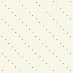
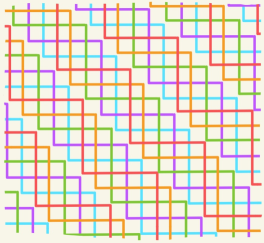
Figure 16. $\mathbb{Q}$-Gorenstein deformation of the Kawamata Lagrangian

Remark 4.2.

The bounding cochain $\mathfrak{b}$ is illustrated on the left side of Figure 16, where green dots indicate self-intersection points $w_{i}$ of the Lagrangian $\mathbb{K}$ (which is not shown) such that $t_{i}\neq 0$. The right side of Figure 16 explains our interest in these self-intersection points: a naive surgery deformation of $\mathbb{K}$ as in Figure 7 splits $\mathbb{K}$ into $n$ isotopic Lagrangians, which we will later identify with mirrors of the Hacking vector bundle restricted to the general fiber of the family $\mathscr{E}$.

Proof.

Since $a=nq-1$, its inverse $b\equiv-nq-1\mod n^{2}$. The subword of the Gauss word formed by indices divisible by $n$ is $n(n-1),\ldots,2n,n,n,2n,\ldots,n(n-1)$. It follows that contributions to the differential $dw_{i}$ coming from the hidden algebra $\mathscr{A}_{0}$ (the left side of Figure 14) cancel each other out. It remains to show that contributions coming from the visible polygons (the right side of Figure 14) also cancel each other out. We interpret these polygons as lattice rectangles in $\mathbb{Z}^{2}$. The contribution to the differential $dw_{\alpha}$ from a lattice rectangle is trivial unless both NE and SW corners of the rectangle are green or orange. In other words, these corners should belong to colored anti-diagonals from the left side of Figure 16. Furthermore, apart from these two corners, the lattice rectangles should not contain any orange points. We claim that these permitted rectangles come in pairs as illustrated in Figure 17 (left and middle).

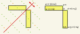
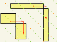
Figure 17. Permitted rectangles come in pairs

.

Here both rectangles have shape $x\times y$. Indeed, if the NE and SW corners of the top rectangle are green or orange then $\alpha\equiv y\equiv-x\mod n$, which implies that these corners of the bottom rectangle are green or orange, and vice versa. Furthermore,

$$\alpha+x-y(1-nq)\equiv\alpha-y+x(1-nq)\mod n^{2},$$ (14)

i.e. $w_{\alpha+x-y(1-nq)}=w_{\alpha-y+x(1-nq)}$. So both rectangles contribute $\bar{w}_{\alpha+x-y(1-nq)}$ to the differential $dw_{\alpha}$ with coefficients that will be determined below.

Next, we claim that if one of the rectangles is not permitted then the other one is not permitted as well. In other words, if one of the rectangles contains orange dots (away from the NE and SW corners) then the other one does as well, as illustrated on the right side of Figure 17. Indeed, suppose the top rectangle contains an orange dot. We slide this point anti-diagonally (in the SE direction) until it hits the bottom rectangle. We claim that one of the dots on this anti-diagonal within the bottom-right rectangle is orange. In order to find this orange dot, we decompose the SE translation as illustrated on the right side of Figure 17. Namely, we first move to the right, hopping from one anti-diagonal of green/orange dots to the next, until we get the point that can be moved down into the bottom-right rectangle. This point will be orange.

Finally, we have to check that if both rectangles in the pair are permitted then the contributions to the differential $dw_{\alpha}$ given by the NW corner of the top rectangle and the SE corner of the bottom rectangle cancel each other out. Concretely, we need to check that

$$[\alpha-y]+[\alpha+x-nqx]+n^{2}\ (\hbox{\rm where we only add $n^{2}$ if}\ [\alpha+x-nqx]=0)$$ (15)

$$=[\alpha-y+nqy]+[\alpha+x]+n^{2}\ (\hbox{\rm where we only add $n^{2}$ if}\ [\alpha+x]=0)$$

Note that, if $y>n$, the condition (15) is invariant under the change $y\mapsto y-n$, which corresponds to shortening the rectangles. Indeed, this obviously preserves permissibility of the rectangles. Furthermore, the left hand side of (15) increases by $n$ (note that $[\alpha-y+n]\neq 0$ since otherwise the bottom rectangle is not permissible), and the same is true for the right hand side. We also claim that, if $x>n$, we can shorten the rectangles in the other direction, $x\mapsto x-n$. Again, this obviously preserves permissibility of the rectangles. We claim that both sides of (15) decrease by $n$ under this operation. Indeed, neither $[\alpha+(x-n)]$ nor $[\alpha+(x-n)-nq(x-n)]$ is equal to $0$ by permissibility of the rectangles. Furthermore, if either $[\alpha+x]$ nor $[\alpha+x-nqx]$ is equal to $0$ then the formula works because $n^{2}$ is added to the formula to compensate.

By the above, we can assume that $x,y\leq n$. Since $\alpha\equiv y\equiv-x\mod n$, $x+y=n$ or $2n$. The second case is, however, impossible because then $x=y=n$ and every $n\times n$ square with green or orange vertices contains orange along the anti-diagonal, which is not permitted. So $0<x<n$ and $y=n-x$. We rewrite (15) as follows:

$$[\alpha-n+x]+[\alpha+x-nqx]+n^{2}\ (\hbox{\rm where we only add $n^{2}$ if}\ [\alpha+x-nqx]=0)$$ (16)

$$=[\alpha-n+x-nqx]+[\alpha+x]+n^{2}\ (\hbox{\rm where we only add $n^{2}$ if}\ [\alpha+x]=0)$$

But this is clear:

$$[\alpha-n+x]=[\alpha+x]-n+n^{2}\ (\hbox{\rm where we only add $n^{2}$ if}\ [\alpha+x]=0),$$

and

$$[\alpha-n+x-nqx]=[\alpha+x-nqx]-n+n^{2}\ (\hbox{\rm where we only add $n^{2}$ if}\ [\alpha+x-nqx]=0).$$

This completes the proof. ∎

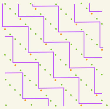
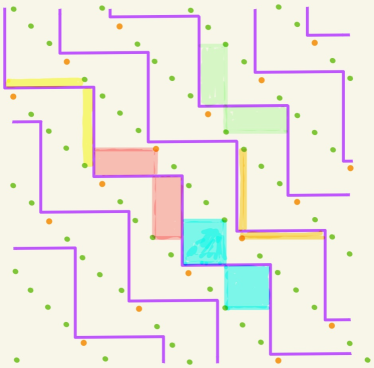
Figure 18. The Hacking Lagrangian $\mathbb{H}_{n,q}$ (left) and Lemma 4.5 (right).

The relative Fukaya category $\mathcal{F}(\mathbb{T}_{1},\{s\})$ is s $k[s]$-linear triangulated category. Its base change $\mathcal{F}(\mathbb{T}_{1},\{s\})\otimes_{k[s]}k[s^{\pm 1}]$ corresponds under mirror symmetry to the category of perfect complexes on the complement of the special fiber of the family $\mathscr{E}\to\mathbb{A}^{1}_{s}$. Motivated by Figure 16, we define an object $\mathbb{H}\in\mathcal{F}(\mathbb{T}_{1},\{s\})\otimes_{k[s]}k[s^{\pm 1}]$. We will show in Lemma 4.4 that its specialization to any $s\neq 0$ is a mirror of the Hacking vector bundle $\mathcal{H}|_{\mathscr{E}_{s}}$ (up to tensoring with a degree $0$ line bundle).

Definition 4.3.

Let the Hacking Lagrangian $\mathbb{H}:=\mathbb{H}_{n,q}$ be a Lagrangian illustrated (on the universal cover of the torus) in Figure 18 and equipped with a local system over $k[s^{\pm 1}]$ whose monodromy is given by $s^{-1}$. Note that $\mathbb{H}$ has one “vertical” and one “horizontal” segment. When doing computations for a Lagrangian endowed with a local system, one trivializes the local system on outside of a specified marked point, which we put near the orange dot where $\mathbb{H}$ bends. Holomorphic curve counts are twisted by the monodoromy of the local system whenever the boundary of the holomorphic polygon passes through this marked point.

Lemma 4.4.

For $s\neq 0$, the specialization $\mathbb{H}_{s}$ of the Hacking Lagrangian is the mirror of the restriction of the Hacking vector bundle $\mathcal{H}|_{\mathscr{E}_{s}}$ tensored with a degree $0$ line bundle.

Proof.

Let $\mathcal{H}_{s}\in\mathrm{Perf}(\mathscr{E}_{s})$ be an object that corresponds to $\mathbb{H}_{s}$ under homological mirror symmetry. Using Figure 6, we compute ${\mathop{\hbox{\rm{RHom}}}}(\mathcal{H}_{s},\mathcal{O}_{q})=k^{n}$ for every closed point $q\in\mathscr{E}_{s}$. So $\mathcal{H}_{s}$ is a vector bundle of rank $n$. A surgery illustrated on the right side of Figure 17 shows that $c_{1}(\mathcal{H}_{s})=\frac{1}{n}c_{1}(\mathcal{F}|_{\mathscr{E}_{s}})$. By (13), it follows that $\mathcal{H}_{s}$ and $\mathcal{H}|_{\mathscr{E}_{s}}$ are vector bundles of the same rank and degree on the $1$-nodal cubic curve $\mathscr{E}_{s}$. In fact, using Figure 6 and homological mirror symmetry, we see that $R\Gamma(\mathscr{E}_{s},\mathcal{H}_{s})=k^{q}$ and $R\Gamma(\mathscr{E}_{s},\mathcal{F}|_{\mathscr{E}_{s}})=k^{nq}$. In particular, $\deg\mathcal{H}_{s}=\deg\mathcal{H}|_{\mathscr{E}_{s}}=q$ by Riemann-Roch. Since both $\mathcal{H}|_{\mathscr{E}_{s}}$ and $\mathcal{H}_{s}$ are simple vector bundles (here we use (13) for $\mathcal{H}|_{\mathscr{E}_{s}}$ and homological mirror symmetry for $\mathcal{H}_{s}$), they are both stable and isomorphic up to tensoring with a degree $0$ line bundle [3]. ∎

Next, we work with the category $\mathcal{F}(\mathbb{T}_{1},\{s\})\otimes_{k[s]}k[t]$ where $s=t^{n}$. We view the Kawamata Lagrangian $\mathbb{K}$ endowed with a bounding cochain $\mathfrak{b}$ of Lemma 4.1 as an object $\mathbb{K}_{\mathfrak{b}}$ of this category.

Lemma 4.5.

We can pullback both $\mathbb{K}_{\mathfrak{b}}$ and the Hacking Lagrangian $\mathbb{H}$ to the category $\mathcal{F}(\mathbb{T}_{1},\{s\})\otimes_{k[s]}k[t^{\pm 1}]$. Then ${\mathop{\hbox{\rm{Hom}}}}(\mathbb{K}_{\mathfrak{b}},\mathbb{H})\cong k[t,t^{-1}]^{\oplus n}$.

Proof.

In Figure 16, the Kawamata Lagrangian (which is not shown) follows the grid (which includes orange and green points), while the Hacking Lagrangian goes halfway between the lines of the grid. It follows that the Kawamata and Hacking Lagrangians intersect in $n$ points along the vertical segment of the Hacking Lagrangian and $n$ points along its horizontal segment. This will show that ${\mathop{\hbox{\rm{Hom}}}}(\mathbb{K}_{\mathfrak{b}},\mathbb{H})\cong k[t,t^{-1}]^{\oplus n}$ if we can prove that the differentials in the $A_{\infty}$-module $CF(\mathbb{K}_{\mathfrak{b}},\mathbb{H})$ vanish. The proof is the same as the proof of Lemma 4.1: contributions to each differential come in pairs of permitted rectangles (illustrated on the right side of Figure 18), which cancel each other out. Concretely, in the notation of the proof of Lemma 4.1 (see Figure 17), the permitted rectangles have parameters $\alpha=y-nqy$ and $x+y=n$. Instead of (15), the cancellation condition becomes

$$[\alpha-y]=-n+[\alpha+x]+n^{2}\ (\hbox{\rm where we only add $n^{2}$ if}\ [\alpha+x]=0.)$$

Two of the terms in the formula (15) do not appear in our case because the Hacking Lagrangian bends where the Kawamata Lagrangian intersects itself. Also, a new term of $-n$ appears because the local system of the Hacking Lagrangian contributes to the top rectangle of each pair. After simplification, the condition becomes $[-nqy]=-n+[n-nqy]+n^{2}$, where we only add $n^{2}$ if $[n-nqy]=0$. This identity is straightforward. ∎

Lemma 4.6.

Action of $\mathcal{R}={\mathop{\hbox{\rm{End}}}}(\mathbb{K}_{\mathfrak{b}})$ on ${\mathop{\hbox{\rm{Hom}}}}(\mathbb{K}_{\mathfrak{b}},\mathbb{H})\cong k[t,t^{-1}]^{\oplus n}$ gives a $k[t]$-linear map $\mathcal{R}\to{\mathop{\hbox{\rm{Mat}}}}_{n}(k[t])$ that sends an element $\sum\limits_{k\in\mathbb{Z}_{n^{2}}}a_{k}w_{k}\in\mathcal{R}$ to a matrix $A\in{\mathop{\hbox{\rm{Mat}}}}_{n}(k[t])$ with the matrix entries given in Theorem 1.10.

Proof.

We study the product ${\mathop{\hbox{\rm{Hom}}}}(\mathbb{K}_{\mathfrak{b}},\mathbb{H})\otimes{\mathop{\hbox{\rm{Hom}}}}(\mathbb{K}_{\mathfrak{b}},\mathbb{K}_{\mathfrak{b}})\to{\mathop{\hbox{\rm{Hom}}}}(\mathbb{K}_{\mathfrak{b}},\mathbb{H})$ using the basis $\{e_{1},\ldots,e_{n}\}$ of ${\mathop{\hbox{\rm{Hom}}}}(\mathbb{K}_{\mathfrak{b}},\mathbb{H})$ given by red dots in Figure 19 (where only the Hacking Lagrangian $\mathbb{H}$ is shown). The corresponding matrix $A\in{\mathop{\hbox{\rm{Mat}}}}_{n}(k[t])$ is computed using the holomorphic polygons illustrated in Figure 19.

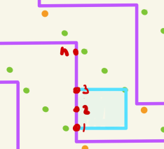
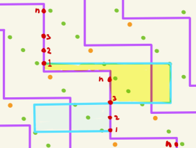
Figure 19. Matrix entries $A_{ij}$ for $i>j$ (left) and $i<j$ (right)

.

When $i>j$, there is only one possibility: the polygon is a rectangle (possibly degenerated into a triangle) with the west side given by points $e_{i}$ and $e_{j}$, the NE corner either green or orange, and no other orange points. The SE corner is a basis element $w_{k}$ of ${\mathop{\hbox{\rm{Hom}}}}(\mathbb{K}_{\mathfrak{b}},\mathbb{K}_{\mathfrak{b}})$. This is illustrated on the left of Figure 19 (for $A_{31}$).

When $i<j$, there are two possibilities, which explains why the formulas in Theorem 1.10 are more complicated in this case. The first possibility, analogous to the case of $i>j$, is to take a rectangle (possibly degenerated into a triangle) with the east side given by points $e_{i}$ and $e_{j}$, the SW corner either green or orange, and no other orange points. The NW corner gives a basis element $w_{k}$ of ${\mathop{\hbox{\rm{Hom}}}}(\mathbb{K}_{\mathfrak{b}},\mathbb{K}_{\mathfrak{b}})$. This is illustrated by a blue rectangle on the right of Figure 19 (for $A_{13}$).

The second possibility is to take a rectangle that starts at the point $e_{i}$, goes to the right along the Kawamata Lagrangian until a green (or orange point), goes down to a self-intersection point $w_{k}$ and then goes to the left to the point $e_{j}$. On the universal cover $e_{j}$ and $e_{i}$ are located on consecutive vertical parts of the Hacking Lagrangian. This is illustrated by a yellow rectangle on the right side of Figure 19 (for $A_{13}$). As always, the rectangle should not contain any orange points except, possibly, the NE corner. The calculation of this composition includes a contribution from the local system on the Hacking Lagrangian.

Finally, contributions to $A_{ij}$ for $i=j$ are given by invisible polygons. The calculation here is entirely analogous to the proof of Corollary 3.5. ∎

It remains to prove the following lemma:

Lemma 4.7.

Under homological mirror symmetry, the Lagrangian $\mathbb{K}_{\mathfrak{b}}$ corresponds to the restriction $\mathcal{F}|_{\mathcal{E}}$ of the Kawamata vector bundle $\mathcal{F}$ on the $\mathbb{Q}$-Gorenstein deformation $\mathcal{W}$ of $W$ to the family of genus $1$ curves $\mathcal{E}\subset\mathcal{W}$ (up to tensoring with a line bundle).

Proof.

Let $\mathcal{K}=\mathcal{F}|_{\mathcal{E}}$ and let $\mathcal{K}^{\prime}\in\mathrm{Perf}(\mathcal{E})$ be an object that corresponds to $\mathbb{K}_{\mathfrak{b}}$ under homological mirror symmetry. Both $\mathcal{K}^{\prime}$ and $\mathcal{K}$ are deformations of the same vector bundle $F|_{E}$ on the special fiber $E\cong E_{2}$ of $\mathcal{E}$. In particular, $\mathcal{K}^{\prime}$ and $\mathcal{K}$ are vector bundles of the same rank $n^{2}$ and degree $nq$. It suffices to show that $\mathcal{K}^{\prime}_{t}$ and $\mathcal{K}_{t}$ are isomorphic up to tensoring with a line bundle for every $t\neq 0$. As in Lemma 4.4, let $\mathcal{H}_{t}$ be the vector bundle that corresponds to the Lagrangian $\mathbb{H}$ under mirror symmetry. By Lemma 4.4 and (13), it suffices to prove that $\mathcal{K}^{\prime}_{t}\cong\mathcal{H}_{t}^{\oplus n}$. By Lemma 4.5 and mirror symmetry, we have ${\mathop{\hbox{\rm{Hom}}}}(\mathcal{K}^{\prime}_{t},\mathcal{H}_{t})\cong k^{\oplus n}$. It follows that ${\mathop{\hbox{\rm{Hom}}}}(\mathcal{H}_{t},\mathcal{K}^{\prime}_{t})\cong\mathop{\hbox{\rm{Ext}}}^{1}(\mathcal{K}^{\prime}_{t},\mathcal{H}_{t})^{*}\cong k^{\oplus n}$ since $\mathcal{K}^{\prime}_{t}$ and $\mathcal{H}_{t}$ have the same slope. By Lemma 4.8, it suffices to prove that the bilinear pairing

$${\mathop{\hbox{\rm{Hom}}}}(\mathcal{K}^{\prime}_{t},\mathcal{H}_{t})\otimes{\mathop{\hbox{\rm{Hom}}}}(\mathcal{H}_{t},\mathcal{K}^{\prime}_{t})\to k,\quad e\otimes f\mapsto e\circ f\in{\mathop{\hbox{\rm{Hom}}}}(\mathcal{H}_{t},\mathcal{H}_{t})=k$$

is non-degenerate. Let $e_{1},\ldots,e_{n}\in{\mathop{\hbox{\rm{Hom}}}}(\mathbb{K}_{\mathfrak{b}},\mathbb{H})$ be the basis used in the proof of Lemma 4.6 (represented by red dots in Figure 20). Let $\mathbb{H}^{\prime}$ is a small perturbation of the Hacking Lagrangian $\mathbb{H}$ and let $f_{1},\ldots,f_{n}\in{\mathop{\hbox{\rm{Hom}}}}(\mathbb{H}^{\prime},\mathbb{K}_{\mathfrak{b}})$ be a basis represented by blue dots in Figure 20. As this picture illustrates, these bases are dual under the bilinear pairing since the only rectangles contributing to the composition are the obvious black rectangles illustrated in this picture. ∎

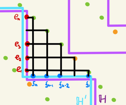
Figure 20. Dual bases in ${\mathop{\hbox{\rm{Hom}}}}(\mathbb{K},\mathbb{H})$ and ${\mathop{\hbox{\rm{Hom}}}}(\mathbb{H}^{\prime},\mathbb{K})$

.

Lemma 4.8.

Let $H$ be a simple vector bundle on a $k$-scheme $X$. Let $K$ be a vector bundle such that $\mathop{\hbox{\rm{rk}}}K=n\mathop{\hbox{\rm{rk}}}H$ for some integer $n$. Then $K$ is isomorphic to $H^{\oplus n}$ if and only if ${\mathop{\hbox{\rm{Hom}}}}(K,H)$ and ${\mathop{\hbox{\rm{Hom}}}}(H,K)$ are $n$-dimensional vector spaces and the bilinear pairing

$${\mathop{\hbox{\rm{Hom}}}}(K,H)\otimes{\mathop{\hbox{\rm{Hom}}}}(H,K)\to k,\quad e\otimes f\mapsto e\circ f\in{\mathop{\hbox{\rm{Hom}}}}(H,H)=k$$

is non-degenerate.

Proof.

The condition is certainly necessary. To show that it is sufficient, we choose dual bases $e_{1},\ldots,e_{n}\in{\mathop{\hbox{\rm{Hom}}}}(K,H)$ and $f_{1},\ldots,f_{n}\in{\mathop{\hbox{\rm{Hom}}}}(H,K)$. Then the morphism $H^{\oplus n}\to H^{\oplus n}$ given by the matrix $e_{i}\circ f_{j}$ for $i,j=1,\ldots,n$ is an identity isomorphism. But it factors through the morphism $e:\,K\to H^{\oplus n}$ given by $e=(e_{1},\ldots,e_{n})$. It follows that $e$ is a surjective morphism of locally free sheaves of the same rank. Therefore, $e$ is an isomorphism. ∎

Proof of Proposition 1.11.

Instead of using explicit formulas, we use presentation of the order from Corollary 3.5. Recall that $s=t^{n}$. Setting $\tilde{w}_{i}=w_{i}/s$ for $i\neq 0$ and $\tilde{w}_{0}=w_{0}$ in the formulas from Corollary 3.5 shows that the only products that survive in the limit as $t^{\prime}=1/t\to 0$ are the products $w_{j}w_{i}=sw_{k}$ appearing in the third polygon from the top, which in the limit become $\tilde{w}_{j}\tilde{w}_{i}=\tilde{w}_{k}$.This algebra is isomorphic to $R_{n^{2},nq-1}$ via an isomorphism $\tilde{w}_{i}\mapsto w_{-i}$. ∎

References

[1] M. Abouzaid, On the Fukaya Categories of Higher Genus Surfaces,
Adv. in Math. 217 (2008), 1192–1235
[2] K. Behnke, J.A. Christophersen, M-Resolutions and Deformations of Quotient Singularities, American Journal of Mathematics 116 (1994), 881–903
[3] I.I. Burban, Stable Bundles on a Rational Curve with One Simple Double Point,
Ukrainian Mathematical Journal 55 (2003), 1043–1053
[4] R.-O. Buchweitz, Maximal Cohen-Macaulay modules and Tate cohomology,
Mathematical Surveys and Monographs, AMS, Providence, RI, 2021, vol. 262, pp. xii+175
[5] K. Fukaya, Y.-G. Oh, H. Ohta, K. Ono,
Lagrangian intersection Floer theory: anomaly and obstruction, Part I, American Mathematical Society, 2010
[6] P. Hacking, Exceptional bundles associated to degenerations of surfaces,
Duke Math. Journal 162 (2013), 1171–1202.
[7] P. Hacking, J. Tevelev, G. Urzúa, Flipping surfaces,
J. Alg. Geom. 26 (2017), 279–345
[8] L. Hille, D. Ploog, Tilting chains of negative curves on rational surfaces,
Nagoya Math. Journal 235 (2019), 26–41
[9] M. Kalck, J. Karmazyn, Non-commutative Knörrer type equivalences via non-commutative resolutions of singularities, arXiv:1707.02836
[10] M. Kalck, J. Karmazyn, Ringel duality for certain strongly quasi-hereditary algebras,
European Journal of Mathematics 4, (2018), 1100–1140
[11]
J. Karmazyn, A. Kuznetsov, E. Shinder,
Derived categories of singular surfaces,
J. Eur. Math. Soc. 24, (2022) 461–526.
[12] Y. Kawamata,
On multi-pointed non-commutative deformations and Calabi–Yau threefolds,
Compositio Mathematica, 154 (2018), 1815–1842.
[13] Y. Kawamata, Semi-orthogonal decomposition and smoothing,
J. Math. Sci. U. Tokyo, 31 (2024), 127-185
[14]J. Kollár, N.I. Shepherd-Barron,
Threefolds and deformations of surface singularities, Invent. Math., 91 (1988), 299–338
[15] A. Kuznetsov, E. Shinder,
Categorical absorptions of singularities and degenerations,
Épijournal de Géométrie Algébrique (2024)
[16] Y. Lekili, A. Polishchuk, Arithmetic mirror symmetry for genus
curves with marked points, Selecta Mathematica 23 (2017), 1851–1907.
[17] Y. Lekili, A. Polishchuk, Auslander orders over nodal stacky curves and partially wrapped Fukaya categories, Journal of Topology 11 (2018), 615–644
[18] Y. Lekili, T. Perutz, Fukaya categories of the torus and Dehn surgery,
PNAS 108 (2011), 8106–8113
[19] Y. Lekili, J. Tevelev, Computer code implementation of Corollary 3.5,
available upon request
[20] D. Orlov, Triangulated categories of singularities and D-branes in Landau-Ginzburg models,
Algebraic geometry: Methods, relations, and applications, Tr.
Mat. Inst. Steklova 246 (2004), 240–262.
[21] H. C. Pinkham, Deformations of algebraic varieties with action,
Astérisque,
Société mathématique de France,
20 (1974)
[22]
P. Seidel, Homological mirror symmetry for the genus two curve,
J. Alg. Geom. 20 (2011), 727–769
[23] P. Seidel, Fukaya categories and Picard–Lefschetz theory,
European Mathematical Society (EMS), Zürich, 2008, vii+326 pp.
[24] J. Tevelev, G. Urzúa, Categorical aspects of the Kollár–Shepherd-Barron correspondence, 2022, 44 pp., arXiv:2204.13225.
[25] J. Wunram, Reflexive modules on cyclic quotient surface singularities,
LNM 1273 (1987)