Combinatorial Amplitude Patterns via Nested Quantum Affine Transformations

Abstract

This paper introduces a robust and scalable framework for implementing nested affine transformations in quantum circuits. Utilizing Hadamard-supported conditional initialization and block encoding, the proposed method systematically applies sequential affine transformations while preserving state normalization. This approach provides an effective method for generating combinatorial amplitude patterns within quantum states with demonstrated applications in combinatorics and signal processing. The utility of the framework is exemplified through two key applications: financial risk assessment, where it efficiently computes portfolio returns using combinatorial sum of amplitudes, and discrete signal processing, where it enables precise manipulation of Fourier coefficients for enhanced signal reconstruction.

I Introduction

Affine transformations combine linear transformations and translations as $A\Psi+B$, where $\Psi\in\mathbb{R}^{N}$ is the input vector, $A\in\mathbb{R}^{N\times N}$ is the linear transformation matrix, and $B\in\mathbb{R}^{N}$ is the translation vector. Affine transformations are foundational in machine learning [1] and iterative methods [2] for tasks like image processing, regression problems, and data analysis where the relative positions of elements need to be retained while allowing for scaling, rotation, and shear.

In quantum computing, the implementation of affine transformations presents a challenge because quantum operations are inherently unitary, i.e., $U^{\dagger}U=I$, preserving the norm and reversibility of quantum states. Recent advances have demonstrated multiple approaches for implementing affine transformations in quantum circuits, integrating concepts from classical transformations with quantum principles to achieve efficient and scalable solutions. For instance, one approach proposes encoding pixel positions and employing controlled-NOT gates and adders for operations like scaling, translation, and scrambling, thereby enabling efficient manipulation of quantum-encoded images [3]. Another approach leverages the synthesis of reversible circuits from invertible matrices, using CNOT gates to represent linear transformations and combining them with simple classical elements like NOT and XOR gates for affine shifts [4]. From a more structural perspective, polyhedral models have been utilized to optimize the scheduling and allocation of gates in circuits that apply affine transformations, effectively handling execution dependencies through loop transformations and affine maps [5]. Polyhedral abstractions combined with Integer Linear Programming (ILP) techniques have enabled the derivation of optimal qubit indexing schemes, minimizing gate counts and circuit depths while respecting device constraints [6]. Similarly, quantum circuits that realize affine mappings over finite fields $F_{2^{n}}$ have been explored using modular arithmetic and normal basis representations, yielding efficient and scalable arithmetic circuits [7].

While these works illustrate the potential of implementing affine transformations in quantum settings, there is a need for a scalable theoretical framework that can apply nested affine transformations. One solution to this problem is to rewrite the affine transformation $f(\Psi)=A\Psi+B$ as a purely linear operation suitable for a quantum state and apply it using block encoding and repeat the process. To achieve this, we use homogeneous coordinates by embedding the $N$-dimensional vector $\Psi$ into an $(2N)$-dimensional space and doubling the size of A to create $\tilde{A}$ that contains the translations terms such that:

$$\tilde{\Psi}=\frac{1}{\sqrt{2}}\begin{bmatrix}\Psi\\ 0\\ 0\\ \vdots\\ 1\end{bmatrix}\in\mathbb{R}^{2N},\quad\tilde{A}=\begin{bmatrix}A^{N\times N}&0^{N\times(N-1)}&B^{N\times 1}\\ 0^{N\times N}&I^{N\times N}\end{bmatrix}\in\mathbb{R}^{(2N)\times(2N)}.$$

With this representation, the affine transformation can be expressed as a purely linear transformation in the augmented space $\tilde{f}(\tilde{\Psi})=\tilde{A}\tilde{\Psi}$. Then the $(2N)\times(2N)$ normalized non-unitary matrix $\frac{\tilde{A}}{\alpha}$ can be embedded into a larger $(4N)\times(4N)$ unitary matrix such that

$$U(\tilde{A})=\begin{pmatrix}\tilde{A}&\sqrt{I-\tilde{A}\tilde{A}^{\dagger}}\\ \sqrt{I-\tilde{A}^{\dagger}\tilde{A}}&-\tilde{A}^{\dagger}\end{pmatrix},$$

where $\alpha>0$ is a normalization factor, ensuring that $\|\tilde{A}/\alpha\|\leq 1$ [8, 9, 10]. The encoded unitary can be applied conditionally to the desired number of qubits to produce the affine transformed amplitudes in the quantum state. In this way, block encoding can be combined with linear transformations in augmented spaces to achieve affine transformations of vectors or fields. However, constructing a block-encoding procedure is challenging and becomes increasingly computationally demanding as the matrix size grows. Employing an augmented affine matrix using block encoding leads to a fourfold increase in matrix size, which further complicates the process as it requires sophisticated decomposition methods [11, 12, 13]. This challenge underscores the need for an efficient strategy to perform such affine transformations within a quantum state.

In this paper, we introduce a scalable method for performing nested affine transformations on a field localized within a sub-state of a quantum state. Our approach uses block encoding of $A$ instead of $\tilde{A}$, which leads to only twofold increase in matrix size and employs Hadamard-supported conditional initialization of the translation terms. This method not only facilitates an easy execution of nested affine transformations but also systematically generates combinatorial patterns of additive and subtractive translation elements, effectively accumulating these amplitudes across various sub-states. This opens up possibilities for further quantum computing applications such as quantum combinatorial optimization, signal processing, and quantum machine learning [14, 15, 16]. With recent advancements in quantum computing algorithms for solving differential equations [17, 18, 19], combinatorial optimization through quantum gradient descent [20], quantum approaches to solving solid mechanics problems [21], and plasma simulations [22], a nested algorithm of this nature can offer efficient iterative methods for addressing these complex problems.

The paper is organized as follows. In the next section, we present a simple method for element-wise addition and subtraction in an $n+1$-qubit system. Following this, a step-by-step nested affine transformation method is introduced. The result is then generalized to any number of affine transformations for any number of qubits. Finally, two potential applications are demonstrated: one in discrete signal processing and the other in financial risk assessment.

II Preliminary: Hadamard-supported element-wise addition and subtraction

Several approaches have been developed to achieve arithmetic operations within quantum states using Fourier-arithmetic techniques [23, 24, 25, 26]. However, these methods are either not suitable or applicable for performing arithmetic directly on a large number of field values within a single quantum state while allowing the flexibility to apply extra unitary operations within the quantum circuit. That is why we use amplitudes of quantum states to represent the field values and perform arithmetic on those amplitudes.

A significant challenge in quantum systems is the inability to directly add or subtract bias terms from amplitudes while maintaining normalization. For instance, consider the states:

$$\Psi_{A}=a_{1}\ket{00}+a_{2}\ket{01}+a_{3}\ket{10}+a_{4}\ket{11},\quad\Psi_{B}=b_{1}\ket{00}+b_{2}\ket{01}+b_{3}\ket{10}+b_{4}\ket{11}.$$

If we simply added two sets of amplitudes, we could end up with a state whose total probability amplitude sum exceeds 1:

$$\Psi_{(A+B)}=(a_{1}+b_{1})\ket{00}+(a_{2}+b_{2})\ket{01}+(a_{3}+b_{3})\ket{10}+(a_{4}+b_{4})\ket{11}.$$

However, it is possible to create a quantum state where $a_{i}+b_{i}$ is accumulated over states, scaled by a known factor, using Hadamard-supported conditional initialization as demonstrated in Fig. 1. A similar approach in which $\Psi_{A}$ and $\Psi_{B}$ are sub-states of a quantum states and are conditionally implemented between two Hadamard gate on the ancillary qubit is demonstrated[27]. Here, we leverage conditional initialization, which is often available in quantum computing software development kits like Qiskit. Conditional initialization prepares one sub-state when the ancilla is $|0\rangle$ and other sub-state when the ancilla is $|1\rangle$. Suppose the two quantum states are given by:

$$\Psi_{A}=\sum_{i=1}^{N}a_{i}\ket{i},\quad\Psi_{B}=\sum_{i=1}^{N}b_{i}\ket{i}.$$

The system is prepared with an $(n+1)$-qubit register in the state:

$$\ket{\Psi_{0}}=\ket{0}\otimes\ket{0}^{\otimes n}.$$

Here, the first qubit acts as an ancillary qubit, while the remaining $n$ qubits are the target register that will store the quantum states. A Hadamard gate $H$ is applied to the ancilla, creating an equal superposition of its computational basis states:

$$\ket{\Psi_{1}}=\frac{1}{\sqrt{2}}(\ket{0}+\ket{1})\otimes\ket{0}^{\otimes n}.$$

This superposition ensures that subsequent initialization of the target qubits depends conditionally on the ancilla’s state. Conditional initialization is then applied to the last $n$ qubits. When the ancilla is in $\ket{0}$, the target qubits are prepared in the state $\Psi_{B}$. When the ancilla is in $\ket{1}$, the target qubits are prepared in $\Psi_{A}$. The resulting state becomes:

$$\ket{\Psi_{2}}=\frac{1}{\sqrt{2}}\left(\ket{0}\otimes\Psi_{B}+\ket{1}\otimes\Psi_{A}\right).$$

Finally, a second Hadamard gate is applied to the ancilla, mixing the states and producing:

$$\ket{\Psi_{3}}=\frac{1}{2}\left[\ket{0}\otimes(\Psi_{A}+\Psi_{B})+\ket{1}\otimes(\Psi_{A}-\Psi_{B})\right].$$

Expanding this, the amplitudes of $\Psi_{A}$ and $\Psi_{B}$ are combined:

$$\ket{\Psi_{3}}=\frac{1}{2}\sum_{i=1}^{N}\left[(a_{i}+b_{i})\ket{0}\ket{i}+(a_{i}-b_{i})\ket{1}\ket{i}\right].$$

This final state encodes both the element-wise sum $a_{i}+b_{i}$ and difference $a_{i}-b_{i}$, scaled to preserve normalization.

$$\Qcircuit@C=1em@R=1.2em{\lstick{\ket{0}}&\gate{H}\ctrlo{1}\ctrl{1}\gate{H}\qw\\ \lstick{\ket{0}}\qw\multigate{1}{\Psi_{B}}\multigate{1}{\Psi_{A}}\qw\qw\\ \lstick{\ket{0}}\qw\ghost{\Psi_{B}}\ghost{\Psi_{A}}\qw\qw\\ }$$

Figure 1: Hadamard-supported element-wise addition and subtraction for a three-qubit system, where the first qubit is ancillary and the remaining two qubits are conditionally initialized with $\Psi_{A}$ and $\Psi_{B}$.

This state encodes both the element-wise sum and difference of the amplitudes of $\Psi_{A}$ and $\Psi_{B}$ while preserving normalization. The emphasis on conditional state initialization arises from recent advancements in quantum state initialization algorithms, particularly the divide-and-conquer and top-down approaches. The divide-and-conquer algorithm achieves an exponential reduction in circuit depth, scaling from $O(N)$ in traditional top-down methods to $O(\log_{2}^{2}(N))$ [28, 29]. However, this improvement comes at the cost of increased qubit usage, requiring $O(N)$ ancillary qubits compared to $O(\log_{2}(N))$ qubits in top-down methods [30]. Depending on the requirements and resource constraints, either state initialization technique can be applied conditionally.

III Nested Affine Transformation

In this section, we discuss how to apply a nested affine transformations to an input field that is accumulated over a sub-state of a quantum system. Given a discrete field $\Psi\in\mathbb{R}^{N}$, the objective is to achieve the following series of transformations:

$$\Psi_{\text{final}}=A^{N\times N}_{k}\big{(}\cdots A^{N\times N}_{2}\big{(}A^{N\times N}_{1}\Psi^{N}+B^{N}_{1}\big{)}+B^{N}_{2}\big{)}\cdots+B^{N}_{k}$$

where $A^{N\times N}_{j}$ is an $N\times N$ linear transformation matrix, and $B^{N}_{j}$ is a column translation vector applied at each step $j$. To achieve the final amplitudes for this transformation, accumulated over a sub-state in a quantum circuit, the circuit width must be strategically expanded, along with constructing the unitary representation of each $A_{j}$. Additionally, each $B_{j}$ must be resized appropriately to match the expanded dimensions as demonstrated in the introduction. At each step $j$, the process involves Hadamard-supported element-wise addition and subtraction, followed by conditional initialization of the resulting state with an additional ancillary qubit. These steps ensure the nested application of the affine transformations within the quantum circuit. The complete sequence of operations is outlined as follows:

Step 1: Amplitude Initialization

Starting with an $s$-qubit system $|0\rangle^{\otimes s}$, initialize the re-scaled $X=[x_{1},x_{2},\dots,x_{N}]$ as amplitudes of $\Psi$ to the last $(n)$-qubits.

$$\Psi_{1}\rightarrow\ |0\rangle^{\otimes(s-n)}\otimes\left(\sum_{i=1}^{N}x_{i}|i\rangle\right).$$

Step 2: Apply Unitary Transformation

To apply the first transformation matrix $A_{1}$, we construct a scaled unitary $U_{1,n+1}$ using block encoding. This unitary acts on $n+1$-qubits and transforms the state such that the amplitude corresponding to $|i\rangle$ becomes $x_{i}^{\prime}$. The resulting quantum state is given by:

$$U_{1,n+1}:\quad|0\rangle^{\otimes(s-n-1)}\otimes\left(\sum_{i=1}^{2N}x_{i}^{\prime}|i\rangle\right).$$

This transformation effectively applies $A_{1}$ while preserving the required qubit structure. Note that the unitary $U_{1,n+1}$ is twice the size of $A_{1}$, which expands the qubit space for $x_{i}$ by one additional qubit.

Step 3: Hadamard-supported Addition/Subtraction with $B_{1}$

We apply Hadamard-supported addition and subtraction of ${B_{1}}=[\omega_{1},\omega_{2},\dots,\omega_{2N}]$ on the existing quantum states to perform amplitude arithmetic.

$$\text{H with }B_{1}:\quad|0\rangle^{\otimes(s-n-2)}\otimes\frac{1}{2}\Bigg{(}\sum_{i=1}^{2N}\big{(}x_{i}^{\prime}+\omega_{i}\big{)}|0\rangle\otimes|i\rangle+\sum_{i=1}^{2N}\big{(}x_{i}^{\prime}-\omega_{i}\big{)}|1\rangle\otimes|i\rangle\Bigg{)}.$$

Step 4: Apply Second Unitary Transformation

After expanding $A_{2}$ into the unitary $U_{2,n+3}$, this unitary is applied to the last $n+3$-qubits of the quantum state. The operation transforms the state as follows:

$$U_{2,n+3}:\quad|0\rangle^{\otimes(s-n-3)}\otimes\frac{1}{2}\Bigg{(}\sum_{i=1}^{4N}\big{(}(x_{i}^{\prime}+\omega_{i})^{\prime}\big{)}|0i\rangle+\sum_{i=1}^{4N}\big{(}(x_{i}^{\prime}-\omega_{i})^{\prime}\big{)}|1i\rangle\Bigg{)}.$$

Each application of a Hadamard operation to facilitate addition and subtraction, as well as any unitary transformation involving $A_{i}$, increases the circuit width by one qubit. This iterative process ensures the desired transformation is achieved while systematically expanding the qubit space.

Step 5: Hadamard Addition/Subtraction with $B_{2}$

Apply Hadamard-supported addition and subtraction of $B_{2}=[\beta_{1},\beta_{2},\dots,\beta_{8N}]$ to the quantum state. The transformation modifies the amplitudes as follows:

$$\text{H with }B_{2}:\quad|0\rangle^{\otimes(s-n-4)}\otimes\frac{1}{2}\Bigg{[}\sum_{i=1}^{4N}\left(\frac{(x_{i}^{\prime}+\omega_{i})^{\prime}}{2}+\beta_{i}\right)|0\rangle\otimes|0i\rangle$$

$$+\sum_{i=1}^{4N}\left(\frac{(x_{i}^{\prime}-\omega_{i})^{\prime}}{2}+\beta_{4N+i}\right)|0\rangle\otimes|1i\rangle$$

$$+\sum_{i=1}^{4N}\left(\frac{(x_{i}^{\prime}+\omega_{i})^{\prime}}{2}-\beta_{i}\right)|1\rangle\otimes|0i\rangle$$

$$+\sum_{i=1}^{4N}\left(\frac{(x_{i}^{\prime}-\omega_{i})^{\prime}}{2}-\beta_{4N+i}\right)|1\rangle\otimes|1i\rangle\Bigg{]}.$$

IV Generalized Nested Affine Transformation

By incrementally increasing the quantum system’s width—introducing additional qubits as necessary—and scaling the size of the translation vectors, while constructing unitaries to represent the linear transformations via block encoding, we can iteratively apply k transformations and translations to produce the following quantum state:

$$|\Psi_{\text{final}}\rangle=|0\rangle^{\otimes(s-n-2k)}\otimes\frac{1}{2^{k}}\sum_{b=1}^{2^{k-1}}\sum_{i=1}^{2^{k}N}\left[\sum_{m=1}^{k}\left(\prod_{j=1}^{k}U_{j}\right)S_{b,i}B_{i,k}\right]|\mathbf{b}\rangle\otimes|i\rangle.$$

This expression represents a generalized quantum state constructed through sequential applications of unitary transformations ($U_{j}$) and translations constants ($B_{i,k}$), combined with a structured superposition of sign patterns ($S_{b,i}\in\{+1,-1\}$). The state captures all possible signed combinations of scaled constants, enabling exploration of a vast Hilbert space through a combinatorial structure. The sequential Hadamard-supported operations create a cascading effect, while the normalization factor ensures the state adheres to normalization. Starting from an initial field ($B_{0,i}=\Psi_{initial}$), this framework allows for any number of affine transformation scaled by a constant factor. The overall procedure is summarized in the Algorithm 1.

Algorithm 1 Nested Quantum Affine Transformations

$s,n,k,\Psi_{initial}\in\mathbb{R}^{2^{n}},\{A_{j}\}_{j=1}^{k},\{B_{j}\}_{j=1}^{k}$

$\Psi_{\mathrm{final}}$

Idea: Start with a quantum state encoding $\Psi_{initial}$. For each $j$ from $1$ to $k$, (1) block-encode and apply $A_{j}$ as a unitary $U_{j}$, and (2) perform Hadamard-supported conditional initialization of the resulting state after applying $U_{j}$ and $B_{j}$.

function NESTED_AFFINE_TRANSFORM($\Psi,\{A_{1},\ldots,A_{k}\},\{B_{1},\ldots,B_{k}\},n,s$)

  current_state $\leftarrow\text{INITIALIZE\_AMPLITUDES}(\Psi,n,s)$

  for $j=1$ to $k$ do

   $s\leftarrow s+1$

   $U_{j}\leftarrow\text{BLOCK\_ENCODE}(A_{j},2^{n+2(j-1)})$

   current_state $\leftarrow\text{APPLY\_UNITARY}(U_{j},\text{current\_state})$

   $s\leftarrow s+1$

   $B_{j}^{(\mathrm{exp})}\leftarrow\text{RESCALE}(B_{j},2^{n+2j})$

   current_state $\leftarrow\text{HADAMARD\_SUPPORTED\_ADD\_SUB}(\text{current\_state},B_{j}^{(\mathrm{exp})})$

  end for

  return current_state

end function

V Applications of the Nested Affine Transformation Procedure

V.1 Financial Risk Assessment

A portfolio return $R$, which includes the sign variables $S_{b,i}\in\{-1,1\}$ for each asset and comprises multiple sums over different asset groups, can be expressed as

$$R=\left[\sum_{i}S_{b,i}B_{i,1},\sum_{j}S_{b,j}B_{j,2},\sum_{k}S_{b,k}B_{k,3},\dots\right].$$

Efficient computation of portfolio returns and their associated risks is a fundamental problem in computational finance, and quantum computing offers novel solutions to this challenge [31]. Traditional methods, such as Monte Carlo simulations, become inefficient when capturing tail risks due to the combinatorial explosion caused by $S_{b,i}$, especially in high-dimensional scenarios [32, 33].
We propose a quantum computing approach that constructs a combinatorial summation of amplitudes within a quantum circuit, enabling the simultaneous handling of multiple sums and sign variations [34]. By leveraging the quantum nested affine transformation, all possible combinations of asset returns can be represented simultaneously in a quantum state. Setting all linear transformations $A_{j}$ to the identity matrix highlights the combinatorial nature of the nested additions. In this simplified scenario, the final state directly encodes all possible sign combinations of the translation vectors $B_{j}$, offering a powerful method for exploring the entire risk profile of a portfolio simultaneously:

$$|\Psi_{\text{final}}\rangle=|0\rangle^{\otimes(s-n-2k)}\otimes\frac{1}{2^{k}}\sum_{b=1}^{2^{k-1}}\sum_{i=1}^{2^{k}N}\left[\sum_{m=1}^{k}S_{b,i}B_{i,k}\right]|\mathbf{b}\rangle\otimes|i\rangle.$$

This state encodes all possible combinatorial sums and differences of the coefficients $B_{i,k}$, weighted by the sign factor $S_{b,i}$. Recent advancements in quantum portfolio optimization have shown the potential to significantly accelerate such computations using quantum parallelism [35, 36]. In portfolio management, this enables efficient computation of weighted combinations of asset returns using a constant number of Hadamard-supported conditional initializations. This approach could be extended to solve a variety of optimization problems, including knapsack variants, offering substantial computational advantages[33, 34].

V.2 Discrete Signal Processing

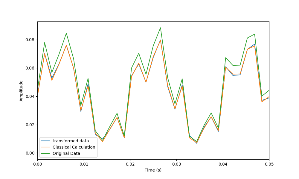
(a)Illustrates the original signal, its classically processed signal (DFT → Affine Transformation → IDFT), and the result of our quantum procedure (QFT → Affine Transformation → Inverse QFT).

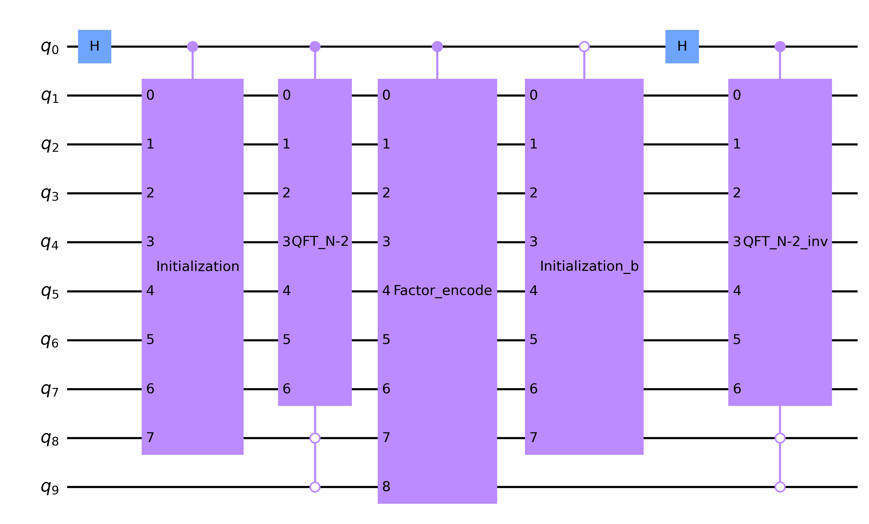
(b) Schematic quantum circuit in Qiskit implementing these steps on a 10-qubit quantum system.

Figure 2: The discrete-time signal $x[n]$ is composed of sinusoidal components with frequencies 50 Hz, 200 Hz, 300 Hz, and 800 Hz, and corresponding amplitudes 1, 0.5, 0.2, and 0.1, respectively. It is defined as $x[n]=\sin(2\pi\cdot 50\cdot t)+0.5\sin(2\pi\cdot 200\cdot t)+0.2\sin(2\pi\cdot 300\cdot t)+0.1\sin(2\pi\cdot 800\cdot t)$, where $t$ represents uniform sampling in time. The signal is fourier transformed, then one affine transformation is applied followed by inverse fourier transformation.

Discrete signal processing techniques are pivotal in enhancing signals, suppressing noise, filtering image and audio data, and enabling efficient data compression [37, 38]. These transformations facilitate precise control of signal properties in both the time and frequency domains. The Discrete Fourier Transform (DFT) of $x[n]$ is given by:

$$X[k]=\sum_{n=0}^{N-1}x[n]e^{-j\frac{2\pi}{N}kn},\quad k=0,1,\ldots,N-1,$$

where $N$ is the signal length, and $X[k]$ represents the complex Fourier coefficients in the frequency domain [39]. To manipulate the signal in the frequency domain, an affine transformation is applied to the Fourier coefficients: $\tilde{X}[k]=a\cdot X[k]+b$, where $a$ is a scaling factor for amplitude modification, and $b$ introduces a constant bias. The modified coefficients are transformed back into the time domain using the Inverse Discrete Fourier Transform (IDFT):

$$\tilde{x}[n]=\frac{1}{N}\sum_{k=0}^{N-1}\tilde{X}[k]e^{j\frac{2\pi}{N}kn},\quad n=0,1,\ldots,N-1.$$

A discrete signal $x[n]=\sum_{i=1}^{L}A_{i}\sin(2\pi f_{i}t),$ where $t$ represents uniform sampling in time, $f_{i}$ are the frequencies, and $A_{i}$ are the corresponding amplitudes of the sinusoidal components is processed as amplitudes of a quantum state, which is followed by Quantum Fourier Transformation (QFT) [40], Affine transformation in frequency domain, and Inverse Fourier Transform as shown in Fig. 2. QFT moves the signals from time domain to the frequency domain, the affine transformation creates a filter and a shift on the frequency coefficients, and then the Inverse QFT returns the signal from the frequency domain to time domain.

This methodology enables precise control over signal characteristics, such as selectively enhancing or suppressing components for applications in audio processing, image filtering, and data compression. Multiple layers of affine transformations could be done in the frequency domain such that different filters are applied in each transformation.

VI Conclusion

In summary, this work presents a scalable and systematic framework for implementing nested affine transformations in quantum circuits. By representing affine transformations in an augmented vector space and using block encoding and Hadamard-supported conditional initialization, the proposed method efficiently generates combinatorial amplitude patterns while maintaining state normalization. The versatility of the approach is demonstrated through potential applications in financial risk assessment, where it efficiently computes portfolio returns using combinatorial sum of amplitudes, and discrete signal processing, where it enables precise manipulation of Fourier coefficients for enhanced signal reconstruction. As quantum computing continues to advance, techniques like nested affine transformations will be increasingly valuable for tackling complex computational tasks spanning optimization, machine learning, signal processing, and beyond. By providing a clear pathway from theoretical constructs to practical, implementable quantum circuits, this work paves the way for more robust and scalable quantum algorithms that can harness the full power of quantum parallelism and combinatorial patterns. Future research could extend this approach to multidimensional transformations and explore its potential in quantum machine learning and combinatorial optimizations.

References

- [1] J. Cao, K. Zhang, H. Yong, X. Lai, B. Chen, and Z. Lin, “Extreme learning machine with affine transformation inputs in an activation function,” IEEE Transactions on Neural Networks and Learning Systems, vol. 30, no. 7, pp. 2093–2107, 2019.
- [2] H. Li, X. Huang, J. Huang, and S. Zhang, “Feature matching with affine-function transformation models,” IEEE Transactions on Pattern Analysis and Machine Intelligence, vol. 36, no. 12, pp. 2407–2422, 2014.
- [3] H. Liang, X. Tao, and N. Zhou, “Quantum image encryption based on generalized affine transform and logistic map,” Quantum Information Processing, vol. 15, no. 7, pp. 2701–2724, 2016.
- [4] X. Zeng, G. Yang, X. Song, M. A. Perkowski, and G. Chen, “Detecting affine equivalence of boolean functions and circuit transformation,” The Computer Journal, vol. 66, pp. 2220–2229, 07 2022.
- [5] M. Kong, “On the impact of affine loop transformations in qubit allocation,” ACM Transactions on Quantum Computing, vol. 2, Sept. 2021.
- [6] B. Gerard and M. Kong, “Exploring affine abstractions for qubit mapping,” in 2021 IEEE/ACM Second International Workshop on Quantum Computing Software (QCS), pp. 43–54, 2021.
- [7] M. Khan and A. Rasheed, “A fast quantum image encryption algorithm based on affine transform and fractional-order lorenz-like chaotic dynamical system,” Quantum Information Processing, vol. 21, no. 134, 2022.
- [8] P. Rall, “Quantum algorithms for estimating physical quantities using block encodings,” Phys. Rev. A, vol. 102, p. 022408, Aug 2020.
- [9] B. D. Clader, A. M. Dalzell, N. Stamatopoulos, G. Salton, M. Berta, and W. J. Zeng, “Quantum resources required to block-encode a matrix of classical data,” IEEE Transactions on Quantum Engineering, vol. 3, pp. 1–23, 2022.
- [10] A. Gilyén, Y. Su, G. H. Low, and N. Wiebe, “Quantum singular value transformation and beyond: exponential improvements for quantum matrix arithmetics,” in Proceedings of the 51st Annual ACM SIGACT Symposium on Theory of Computing, STOC 2019, (New York, NY, USA), p. 193–204, Association for Computing Machinery, 2019.
- [11] D. Camps, L. Lin, R. V. Beeumen, and C. Yang, “Explicit quantum circuits for block encodings of certain sparse matrices,” 2023.
- [12] H. Li, H. Ni, and L. Ying, “On efficient quantum block encoding of pseudo-differential operators,” Quantum, vol. 7, p. 1031, June 2023.
- [13] D. Camps and R. Van Beeumen, “Approximate quantum circuit synthesis using block encodings,” Phys. Rev. A, vol. 102, p. 052411, Nov 2020.
- [14] J. Biamonte, P. Wittek, N. Pancotti, P. Rebentrost, N. Wiebe, and S. Lloyd, “Quantum machine learning,” Nature, vol. 549, pp. 195–202, Sep 2017.
- [15] I. Kerenidis and A. Prakash, “Quantum recommendation systems,” 2016.
- [16] M. Schuld and F. Petruccione, Supervised Learning with Quantum Computers. Quantum Science and Technology, Springer International Publishing, 2018.
- [17] Y. Cao, A. Papageorgiou, I. Petras, J. Traub, and S. Kais, “Quantum algorithm and circuit design solving the poisson equation,” New Journal of Physics, vol. 15, p. 013021, jan 2013.
- [18] A. M. Childs, J.-P. Liu, and A. Ostrander, “High-precision quantum algorithms for partial differential equations,” Quantum, vol. 5, p. 574, Nov. 2021.
- [19] N. Linden, A. Montanaro, and C. Shao, “Quantum vs. classical algorithms for solving the heat equation,” 2020.
- [20] X. Yi, J.-C. Huo, Y.-P. Gao, L. Fan, R. Zhang, and C. Cao, “Iterative quantum algorithm for combinatorial optimization based on quantum gradient descent,” Results in Physics, vol. 56, p. 107204, 2024.
- [21] B. Liu, M. Ortiz, and F. Cirak, “Towards quantum computational mechanics,” Computer Methods in Applied Mechanics and Engineering, vol. 432, p. 117403, Dec. 2024.
- [22] I. Y. Dodin and E. A. Startsev, “On applications of quantum computing to plasma simulations,” Physics of Plasmas, vol. 28, p. 092101, 09 2021.
- [23] L. Ruiz-Perez and J. C. Garcia-Escartin, “Quantum arithmetic with the quantum Fourier transform,” Quantum Information Processing, vol. 16, no. 6, p. 152, 2017.
- [24] T. Häner, M. Roetteler, and K. M. Svore, “Optimizing quantum circuits for arithmetic,” 2018.
- [25] M. K. Thomsen, R. Glück, and H. B. Axelsen, “Reversible arithmetic logic unit for quantum arithmetic,” Journal of Physics A: Mathematical and Theoretical, vol. 43, no. 38, p. 382002, 2010.
- [26] R. Seidel, N. Tcholtchev, S. Bock, C. K.-U. Becker, and M. Hauswirth, “Efficient floating point arithmetic for quantum computers,” IEEE Access, vol. 10, pp. 72400–72415, 2022.
- [27] P. Wittek, Quantum Machine Learning: What Quantum Computing Means to Data Mining. Academic Press, 2014.
- [28] I. F. Araujo, D. K. Park, F. Petruccione, et al., “A divide-and-conquer algorithm for quantum state preparation,” Scientific Reports, vol. 11, p. 6329, 2021.
- [29] D. Ventura and T. Martinez, “Initializing the amplitude distribution of a quantum state,” Foundations of Physics Letters, vol. 12, pp. 547–559, 1999.
- [30] I. F. Araujo, D. K. Park, T. B. Ludermir, et al., “Configurable sublinear circuits for quantum state preparation,” Quantum Information Processing, vol. 22, p. 123, 2023.
- [31] S. Woerner and D. J. Egger, “Quantum risk analysis,” npj Quantum Information, vol. 5, p. 15, 2019.
- [32] P. Rebentrost and S. Lloyd, “Quantum computational finance: Pricing derivatives,” Physical Review A, vol. 98, no. 2, p. 022321, 2018.
- [33] D. J. Egger, S. Woerner, and I. Tavernelli, “Quantum computing for finance: State-of-the-art and future prospects,” npj Quantum Information, vol. 6, p. 1, 2020.
- [34] A. Bouland and S. Gharibian, “On the complexity and applications of quantum portfolio optimization,” Quantum, vol. 4, p. 334, 2020.
- [35] R. Orus, S. Mugel, and E. Lizaso, “Quantum approaches to portfolio optimization,” arXiv preprint arXiv:1811.12344, 2018.
- [36] G. Rosenberg and et al., “Quantum machine learning for credit scoring and risk management,” PLOS One, vol. 14, no. 8, p. e0221304, 2019.
- [37] A. V. Oppenheim and R. W. Schafer, Discrete-Time Signal Processing. Pearson Education, 2009.
- [38] A. Papoulis, “Applications of discrete signal processing in modern technology,” Journal of Applied Signal Processing, vol. 10, no. 3, pp. 210–223, 2012.
- [39] R. N. Bracewell, “A tutorial on fourier transform, discrete fourier transform, and fast fourier transform,” Proceedings of the IEEE, vol. 82, no. 3, pp. 414–428, 1994.
- [40] M. A. Nielsen and I. L. Chuang, Quantum Computation and Quantum Information. Cambridge University Press, 10th anniversary edition ed., 2010.