The Controlled Four-Parameter Method for Cross-Assignment of Directional Wave Systems
Abstract
Cross-assignment of directional wave spectra is a critical task in wave data assimilation. Traditionally, most methods rely on two-parameter spectral distances or energy ranking approaches, which often fail to account for the complexities of the wave field, leading to inaccuracies. To address these limitations, we propose the Controlled Four-Parameter Method (C4PM), which independently considers four integrated wave parameters. This method enhances the accuracy and robustness of cross-assignment by offering flexibility in assigning weights and controls to each wave parameter. We compare C4PM with a two-parameter spectral distance method using data from two buoys moored 13 km apart in deep water. Although both methods produce negligible bias and high correlation, C4PM demonstrates superior performance by preventing the occurrence of outliers and achieving a lower root mean square error across all parameters. The negligible computational cost and customization make C4PM a valuable tool for wave data assimilation, improving the reliability of forecasts and model validations.
Keywords Cross-assignment of wave spectra partitions, Wind-generated waves, Wave spectra assessment, Wave spectra assimilation.
1 Introduction
The wave directional spectrum is the fundamental representation of a sea state, providing a detailed description of the energy distribution as a function of both frequency and direction — hence crucial for understanding the complexities of wave dynamics and interactions. Accurate analysis of the spectrum is vital for various applications, including climate studies, coastal management and maritime safety (Cavaleri et al., 2007; Ardhuin et al., 2019). One of the key challenges is the cross-assignment of spectral partitions, which involves identifying and matching collocated wave systems from different datasets or models — see a discussion about spectral partitioning in Gerling (1992); Violante-Carvalho et al. (2005); Portilla-Yandún et al. (2015, 2019). Cross-assignment is essential for data assimilation, where observational data are integrated into numerical models (Aouf et al., 2006; Hauser et al., 2021), and for assessing measurements, enabling comparison of results from various sources.
Currently, most (if not all) methods for cross-assignment are based either on two-parameter spectral distance or on ranking the energy content of each system — the most energetic partitions in one spectrum are paired to the correspondingly ranked partitions in the other spectrum. Energy ranking methods are more prone to inaccuracies, mainly when the number of partitions of each spectra differ. Cross-assigning only the most energetic partition might overcome this limitation but significantly reduce the possible number of matches. Conversely, methods based on a two-parameter spectral distance rely exclusively on frequency and direction. (see, among many others, Hasselmann et al., 1996; Hanson & Phillips, 2001; Li & Saulter, 2012; Wang et al., 2020; Smit et al., 2021; Aouf et al., 2021; Santos et al., 2021; Jiang et al., 2022; Ricondo et al., 2023; Wu et al., 2024). However, this approach has drawbacks. The main limitation is that it can result in errors, mainly because partitions close in frequency but significantly apart in direction (or vice versa) are mismatched — leading to potential discrepancies caused by outliers. These inaccuracies can propagate through data assimilation processes, resulting in suboptimal model performance and potentially misleading data interpretations.
To overcome these limitations, we propose a novel methodology for cross-assigning partitions, termed the Controlled Four-Parameter Method (C4PM). This approach incorporates four bulk wave spectral parameters: significant wave height, peak wave period, peak wave direction, and peak wave spreading. By independently treating these parameters, the method enhances the robustness and precision of the cross-assignment process, positively affecting the assimilation of observational data into numerical models and thereby improving the forecast results. C4PM has proven to be an valuable and efficient tool to cross-assignment, allowing to define control levels for each of the primary wave parameters and additionally prioritize parameters by assigning weights through a customizable weighting vector.
The structure of the current analysis is organized as follows: Section 2 presents the theoretical framework of C4PM, which includes the definition of the semimetric on which the method is based, as well as a detailed presentation of the cross-assignment scheme used. Section 3 outlines the buoy data and the processing methodologies employed, while Section 4 discusses the results. Finally, the conclusions are summarized in Section 5.
2 The Cross-Assignment Problem
This section addresses the cross-assignment problem, beginning with a basic concept, followed by a brief description of a classic technique and its limitations, and concluding with a detailed explanation of the C4PM method.
2.1 Matching: a fundamental concept
Assuming that and are two measurements of the wavenumber spectrum associated with a certain sea state. After a partitioning process of and , consider the additive decomposition:
| (1) |
where and are, respectively, the partitions111We use the term ”partition” to refer to an independent wave system that is a constituent of the wave spectrum of and . It is supposed from now on that and that the explicit dependence on the wavenumber vector will be omitted.
We call -matching between and a set
| (2) |
formed by of pairs222unordered of partitions of and with the property that no partition of is associated with more than one partition of and vice versa. Ideally, a cross-assignment is a matching between and such that coupled partitions exhibit the highest possible concordance in their oceanic characteristics. Therefore, it is crucial to employ a technique capable of accurately identifying compatible wave systems.
2.2 A two-parameter method (2PM)
Typically, the cross-assignment of spectral partitions heavily relies on evaluating a two-parameter spectral distance. In this context, the fundamental concept behind the technique proposed in Hasselmann et al. (1996) is the association of a partition with its so-called (two-parameter) characteristic wavenumber vector. In that study, the expression
| (3) |
where and are the characteristic wavenumber vectors of and , respectively, was proposed for the distance333the double-bar symbol designates the Euclidean norm between partitions of and . Thus, the -matching given by (2) is the cross-assignment between and , in the Hasselmann sense, if the following conditions are met:
-
(i)
is the largest possible
-
(ii)
-
(iii)
for each .
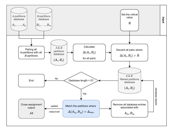
Here, is a specified critical value, which acts as a cutoff line defining which pairs will be in the cross-assignment. Hereafter, we will refer to this technique as 2PM, and its algorithm is illustrated in Figure 1. The method calculates all possible distances between the partitions of and , eliminates pairs with distances exceeding the threshold value , and finally establishes partition matchups by prioritizing the smallest distances.
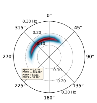
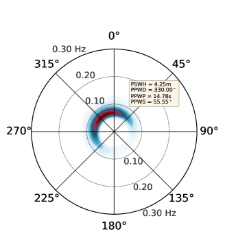
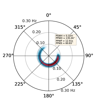
One of the main shortcomings of this approach is that even if the spectral distance between two partitions is considered small — below a given threshold — it does not guarantee a strong agreement between the wave systems they represent. For instance, Hasselmann et al. (1996) suggests that a critical value of yields satisfactory results. However, Figures 2 and 3 illustrate two examples of cross-assigned partitions with distances less than , yet exhibiting significant discrepancies in their wave parameters. In Figure 2, the distance between the partitions is equal to , but the partitioned significant wave height is approximately nine times larger than its assigned counterpart, meaning that unrelated wave systems were associated in the cross-assignment process. A more subtle case of mismatch with distance equal to 0.32 is depicted in Figure 3. Despite similar values of partitioned peak wave periods, partitioned significant wave heights and partitioned peak directional spreadings, the wave systems propagating towards the southern quadrant are separated by 120∘.
2.3 The Controlled Four-Parameter Method - C4PM
As shown in 2.2, 2PM methods for cross-assignment have significant limitations, thereby leaving margin for mismatches in the cross-assignment process. In this context, the Controlled Four-Parameter Method (C4PM) is introduced as a more robust and efficient tool, providing comprehensive control over wave parameter variabilities and their hierarchical importance.
2.3.1 The Weighted Semimetric
A semimetric defined on the partitions of and is a function such that for any and , the following conditions hold: , , and if, and only if, . To define our spectral distance, each partition is associated with a four-dimensional vector whose components represent the partitioned integrated wave parameter values that characterize it: partitioned significant wave height (), partitioned peak wave period (), partioned peak wave direction (), and partioned peak wave spreading (), precisely in that order. This approach incorporates more information about each partition compared to the distance defined in Equation (3). Thus, for each, and , we consider the associations: and , to set our spectral distance (which is a weighted semimetric) between the partitions and as
| (4) |
a dot product, where represents the variability vector, encapsulating the variabilities of the partitioned integrated wave parameters between and , and is the weighting vector, whose components assign weights to each partitioned integrated wave parameter. These vectors are defined as:
| (5) |
where
| (6) |
and
| (7) |
are the variation functions, both bounded above by 1. The weighting vector consists of positive scalars and , which satisfy the condition . It is important to emphasize that the weighting vector offers endless possibilities; for instance, the reliability of the analyzed data serves as a rational criterion for assigning weights to each partitioned integrated wave parameter.
Equation (4) explicitly represents the weighted sum of the partitioned wave parameter variabilities between and , and is given as:
| (8) |
If the weighting vector is balanced, meaning , the distance in Equation (8) simplifies to the arithmetic mean of the variabilities of the partitioned wave parameters. Notably, in contrast to the distance defined by Equation (3), if , then and fully agree in all their corresponding wave parameters, as is a semimetric. Conversely, if , it indicates that at least one corresponding wave parameter between e exhibits a high degree of discrepancy.
2.3.2 A New Cross-Assignment Formulation
In this section, a novel framework for cross-assignment is introduced. Specifically, we demonstrate how the algebraic structure of a weighted semimetric can be employed to regulate the variability of the cross-assigned partitioned integrated wave parameters within a matchup generated by the cross-assignment process. To achieve this, consider a control vector , where each coordinate satisfies . The -matching defined by (2) is referred to as the controlled four-parameter cross-assignment between and , relative to the weighted semimetric and governed by the control vector , if the following conditions are satisfied:
-
(i’)
is the largest possible
-
(ii’)
444the symbol indicates that the components of the variability vector do not exceed the corresponding components of the control vector. for each
-
(iii’)
are valid555the symbols and represent, respectively, the sets of all injective functions from into and from into ..
Condition (ii’) provides control for the cross-assigned partitioned wave parameters of the matchups; the previously chosen constraining scalars , and control the distance between the matched partitions. If the partitions and are -controlled — i.e., condition (ii’) is valid — then the distance between these partitions is
| (9) |
The optimality condition (iii’) characterizes controlled cross-assignment as the matching between and with the shortest possible length. The quantity calculated in (iii’) represents the length of the cross-assignment; among all the -matchings of -controlled partitions of and , this is the one with the smallest length.
If , the cross-assignment problem is unconstrained, and in this case, there is always a solution. Conversely, for instance, if and , there are no constraints on the values of significant wave heights, peak wave directions, or peak directional spreading for the matched partitions. However, a significant constraint is imposed on the values of peak wave periods for the matched partitions. In each matchup, the smallest period is at least of its cross-assigned counterpart. The largest period of that matchup — or in other words, the smallest period is at least 70% of the largest period. In this case, the existence of a constrained cross-assignment depends on the dataset being analyzed. Therefore, an appropriate adjustment of the control vector may be essential to obtain solutions to a controlled cross-assignment problem for a particular data set.
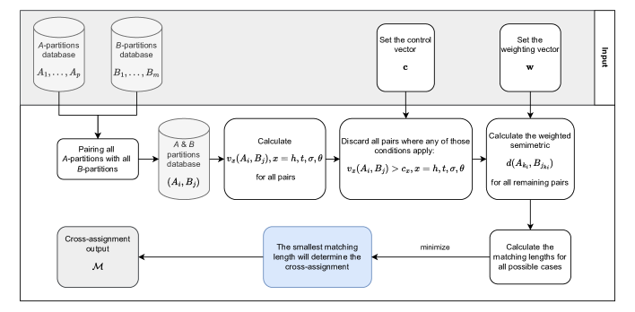
In summary, this section introduced a framework for cross-assignment, which consists of the following: given two partitioned wave spectra (measured) of a specific sea state, the objective is to find the best matching between their spectral partitions, ensuring that the discrepancies in all four partitioned integrated wave parameters are controlled a priori. To address this problem, we developed a computational routine called the Controlled Four-Parameter Method (C4PM), whose diagram is presented in Figure 4. Specifically, we denote the method as u-C4PM when it operates in uniform mode, meaning the control vector is uniform, with .
3 Data and Methods
3.1 NDBC Buoy Data
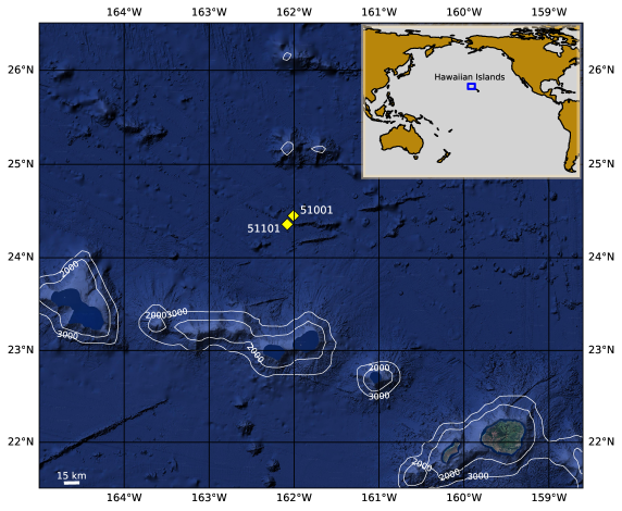
We selected two buoys, operated by the National Data Buoy Center (NDBC), with IDs 51001 and 51101, for the period from January 2023 to December 2023 — details available at https://www.ndbc.noaa.gov/. These buoys are situated approximately 13 km apart in deep water off the coast of Hawaii (Figure 5). Their proximity and location in similar deep-water conditions indicate that both buoys provide relatively comparable measurements. This implies a reasonable number of high-quality pairs can be identified between them, while also reducing challenges associated with applying cross-assignment methodologies, as will be discussed in the following sections. Both buoys collect meteorological and oceanographic data, including the directional wave spectra necessary for cross-assignment techniques. Wave data from these buoys are available at 30 minute intervals, yielding a total of 17,100 pairs of wave spectra (Table 1).
| ID | Latitude | Longitude | Depth |
|---|---|---|---|
| 51001 | 24.451 N | 162.008 W | 4906 m |
| 51101 | 24.359 N | 162.081 W | 4860 m |
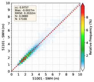
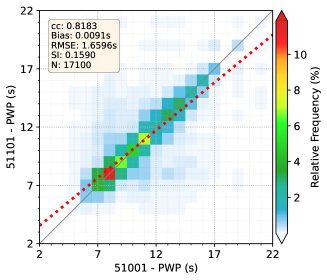
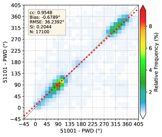
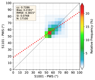
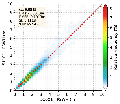
Figure 6 shows, over the selected time period of 2023, the scatter plots of wave parameters: significant wave height , peak wave period , peak wave direction and peak wave spreading . The wave parameters were downloaded directly from the NDBC page — with exception of which was computed as outlined in Table 8 — therefore the spectra were not partitioned. The statistical parameters are listed in Table 7.
As expected, the biases across the four parameters are minimal. However, low-frequency occurrences representing significant differences among the spectral peak pairs are evident, as indicated by the light blue shades, particularly in relation to direction and period (Figure 6b and c). For , the is 0.20 m with a correlation coefficient equal to , indicating a strong level of similarity. Although the agreement for is generally good, numerous outliers in Figure 6b contribute to an increased and lower correlation coefficient. A similar pattern is seen in Figure 6c, where the outliers introduce substantial discrepancies. The lower correlation coefficient among the four wave parameters is associated with , a parameter that is challenging to estimate accurately from single point measurements such as directional buoys (Kuik et al., 1988).
3.2 Data Processing
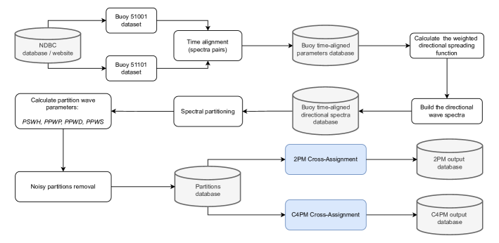
The NDBC provides wave spectral data in the form of five parameters concerning the Fourier series expansion of the buoy’s directional wave spectrum: the non-directional spectral density, the first normalized directional Fourier coefficient, the mean wave direction, the second normalized directional Fourier coefficient and the main wave direction. The time series for each buoy were downloaded for the year 2023. The data are then time-synchronized and consolidated into a database, removing any incomplete entries (i.e. missing data) to ensure that each record has complete information for all five wave parameters from both buoys, at the same date and time. Each row of this database is then processed following Earle et al. (1999), allowing the calculation of the weighted directional spreading function and directional wave spectrum for each buoy. The weighted directional spreading function ensures that the calculated directional wave spectra remain non-negative, addressing potential problems with negative values that can arise when using more basic approaches.
Once the directional wave spectra is obtained, all partitioned integrated wave parameters are calculated as outlined in Table 8, and all noisy partitions are removed according to the following criteria:
-
(a)
m;
-
(b)
s and % .
At this stage, the partition database is consolidated, with the greatest possible amount of matches being 30,956. Both cross-assignment techniques, 2PM and C4PM, were applied to the same dataset, each generating its respective output databases, as illustrated in the processing workflow shown in Figure 7.
4 Results
In general, cross-assignment tasks employ spectra from different sources, such as numerical models, in situ measurements, or remote sensing, which naturally have some degree of discrepancy between them. In many cases, the number of partitions in each paired spectrum differs, with some partitions missing and others being spurious. In these common cases, cross-assignment has to rely heavily on the ability of the employed method to distinguish good matchups. In this sense, some experiments are proposed and analyzed to demonstrate the abilities of C4PM, taking 2PM as a reference.
It is important to note that all C4PM experiments described in this section rely on a balanced weight vector to establish a general approach for comparison with the reference method.
4.1 Sensitivity test
| 2PM: matchups distribution | ||
| 1 | 0.2 | 26213 |
| 2 | 0.4 | 28321 |
| 3 | 0.6 | 29192 |
| 4 | 0.8 | 29654 |
| 5 | 1.0 | 30103 |
| 6 | 1.2 | 30454 |
| 7 | 1.4 | 30649 |
| 8 | 1.6 | 30744 |
| 9 | 1.8 | 30850 |
| 10 | 2.0 | 30956 |
Validating C4PM and assessing its performance is a central issue. To this end, we highlight the parallelism between the roles of the critical value () in 2PM and the control vector () in C4PM. Ultimately, both act as cutoff parameters and, albeit through fundamentally different mechanisms, regulate the distance between partitions matched in each cross-assignment process.
We define the sequence of cutoff values as follows:
| (10) |
for . The -th experiment in this test involves determining the number of matchups and generated by the 2PM and u-C4PM666In uniform mode, the control vector is of the form . runs, respectively, when initialized with input data and . It can be observed that (for the selected dataset) and correspond, in this order, to the maximum possible number of matchups and , both of which are equal to (reached for ). The results are presented in Tables 2 and 3, which highlight a key distinction in the spectral distance behaviors of C4PM and 2PM. Specifically, the distribution of matchups performed by C4PM, as shown in Table 3, exhibits a progressive and scaled increase from the 1st to the 5th metric deciles, followed by a stabilization trend up to the 10th metric decile. In contrast, the distribution of matchups performed by 2PM, according to Table 2, begins with a very high value in the 1st metric decile, with only a relatively small increase observed up to the 10th metric decile. Moreover, the number of matchups in the 1st metric decile of 2PM is remarkably close to the number of matchups in the 4th metric decile of C4PM. Taken together, these observations suggest that the weighted semimetric underlying C4PM offers a superior capability to distinguish between matches. This will become even more apparent in the subsequent sections.
| u-C4PM: matchups distribution | ||
| 1 | 0.1 | 7338 |
| 2 | 0.2 | 18430 |
| 3 | 0.3 | 24112 |
| 4 | 0.4 | 27236 |
| 5 | 0.5 | 29177 |
| 6 | 0.6 | 29915 |
| 7 | 0.7 | 30463 |
| 8 | 0.8 | 30799 |
| 9 | 0.9 | 30919 |
| 10 | 1.0 | 30956 |
4.2 Accuracy test
As a step toward evaluating the performance of C4PM, this test analyzes the results obtained by running the 2PM and u-C4PM algorithms, each initialized with input values that yield the top 0.3% (equivalent to 99 pairs) of the best matchups generated by each technique (Table 4). The input cutoff values were determined and, as expected, are very small: (the critical value for 2PM) and (the control value for u-C4PM). Because the matchups generated by u-C4PM are -uniformly controlled, it follows that, for all cross-assigned partitioned integrated wave parameters (except for partitioned wave peak directions), the smaller parameter is at least 99% of the larger one. Additionally, the partitioned and cross-assigned wave peak directions differ by no more than . In contrast, among the 99 matchups produced by 2PM, 51 pairs exhibit at least one cross-assigned partitioned integrated wave parameter (excluding partitioned wave peak directions) where the smaller parameter is less than 90% of the larger one. For partitioned wave peak directions, the difference in these cases is no less than . These discrepancies are evidently reflected in the RMSEs of the partitioned integrated wave parameters, as summarized in Table 4, and serve to justify the results presented therein. Although the contrasted matchup groups lie within a particularly narrow range, this result highlights a key distinction in the performance of the methods: C4PM successfully prevented the formation of poorly matched partitions, whereas 2PM, even when operating at an extremely low critical value, did not.
| : a strict range | ||||
| Method | (m) | (s) | (∘) | (∘) |
| 2PM | 0.18 | 0.69 | 13.57 | 4.91 |
| u-C4PM | 0.01 | 0.00 | 9.48 | 0.31 |
4.3 A broader comparison
In this test, the largest set of all possible matchups obtained from the u-C4PM and 2PM runs will be divided into quintiles, and their corresponding will be presented and analyzed. To formalize this, let and represent the number of matchups produced by the 2PM and C4PM algorithms, respectively, when initialized with input data and . These cutoff values are defined so that the equations
| (11) |
for are valid.
Tables 5 and 6 summarize the performances of 2PM and C4PM across all quintiles. For both methods, the values of all integrated wave parameters do not consistently decrease with each advancing quintile as the cutoff values progress. Notably, these tables partially reflect the results discussed in 4.2. Consider the first quintile of each method. The 6191 matchups generated by C4PM are -uniformly controlled with . Therefore, for all pairs of cross-assigned integrated wave parameters, the smaller value is at least 91% of the larger one, except for cross-assigned partitioned peak wave directions, whose differences do not exceed . In contrast, these conditions do not hold for the 6191 matchups corresponding to the first quintile under 2PM, as evidenced by their higher values. Specifically, 3647 matches include at least one cross-assigned partitioned integrated wave parameter where the smaller value is less than 91% of the larger one, excluding wave peak directions, which differ by at least . This discrepancy accounts for the higher values observed for 2PM compared to C4PM within this quintile.
| 2PM: per quintile | ||||||
|---|---|---|---|---|---|---|
| (m) | (s) | (∘) | (∘) | |||
| 1 | 20% | 0,0044 | 0.22 | 0.72 | 13.17 | 4.59 |
| 2 | 40% | 0,0142 | 0.23 | 0.76 | 14.81 | 5.00 |
| 3 | 60% | 0,0415 | 0.26 | 0.81 | 17.11 | 5.63 |
| 4 | 80% | 0,1420 | 0.29 | 0.92 | 20.24 | 6.81 |
| 5 | 100% | 2,0000 | 0.32 | 1.80 | 34.74 | 9.22 |
| u-C4PM: per quintile | ||||||
|---|---|---|---|---|---|---|
| (m) | (s) | (∘) | (∘) | |||
| 1 | 20% | 0.0851 | 0.11 | 0.00 | 9,48 | 2.23 |
| 2 | 40% | 0.1266 | 0.15 | 0.72 | 9,70 | 2.92 |
| 3 | 60% | 0.2050 | 0.20 | 0.74 | 13,28 | 4.05 |
| 4 | 80% | 0.3258 | 0.26 | 0.90 | 17,08 | 5.78 |
| 5 | 100% | 1.0000 | 0.31 | 1.65 | 34,71 | 8.50 |
An analogous analysis can be performed for subsequent quintiles, yielding similar conclusions, while noting that the values become increasingly similar as the quintiles progress. The additional, more visual representation of the evolution of values against the percentage of matchups for each experiment — shown in Figure 8 — further corroborates this observation. In particular, the figure demonstrates that C4PM outperformed 2PM in forming matches, regardless of the percentage of total matches considered. In other words, C4PM consistently produced more accurate matchups.
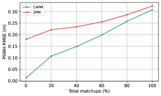
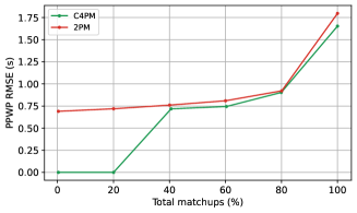
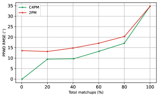
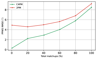
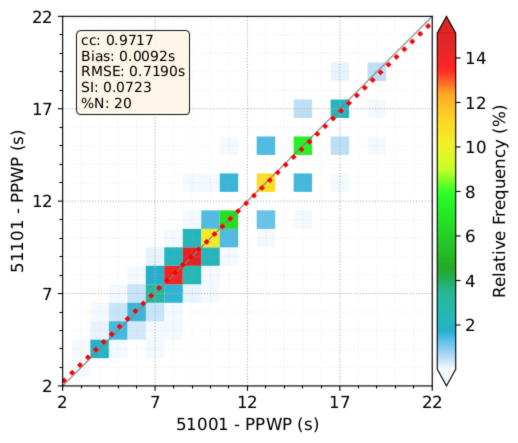
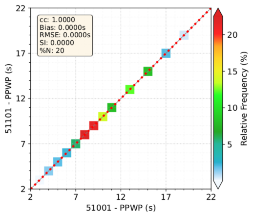
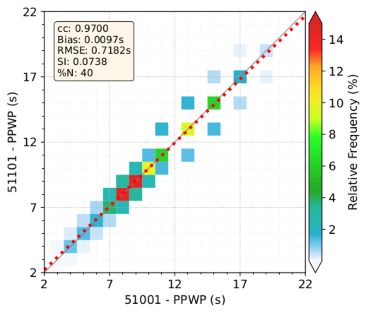
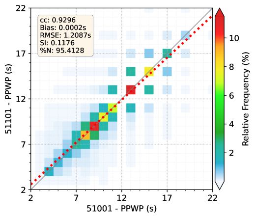
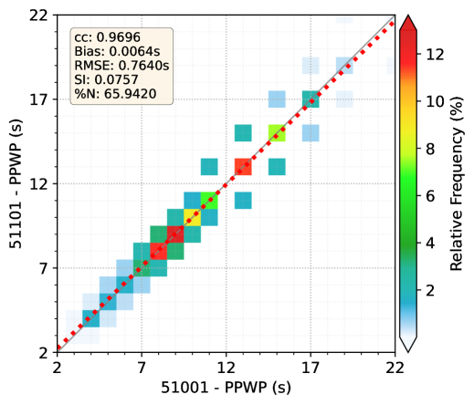
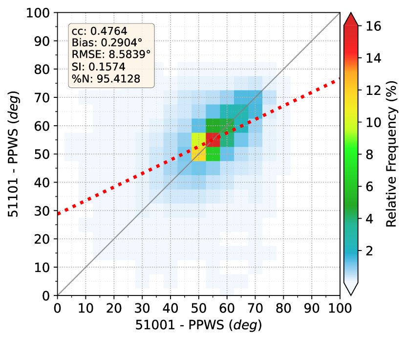
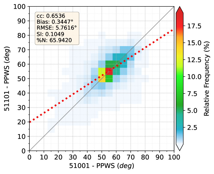
Figure 9 illustrates the PPWP evolution for C4PM and 2PM across the first and second quintiles. In the first quintile, C4PM exhibits a concentrated distribution along the diagonal, indicative of accurate matches and the absence of outliers. Conversely, 2PM demonstrates a more dispersed distribution, with significant outliers reflecting lower match quality. In the second quintile, this trend persists. C4PM continues to maintain a narrow distribution along the diagonal, highlighting its ability to generate reliable matches. In contrast, 2PM displays a broader distribution accompanied by many outliers, further emphasizing its inferior match quality. These observations align with the values reported in Tables 5 and 6. A lower global generally corresponds to improved match quality and fewer outliers, particularly under stricter matching conditions. The consistent superior performance of C4PM in both quintiles underscores its robustness and reliability in producing accurate matches, even under challenging scenarios.

4.4 Two settings confronted
The results obtained from running the 2PM and C4PM algorithms on relatively broad input data are compared. This test does not aim to identify equivalent configurations between the two methods — if such equivalence is even possible — but rather to analyze the behavior of C4PM and the results it produces. Notably, this comparison underscores one of C4PM’s key capabilities: its ability to independently control discrepancies between cross-assigned partitioned integrated wave parameters of different natures, depending on the application, type of measurement, or desired level of accuracy.
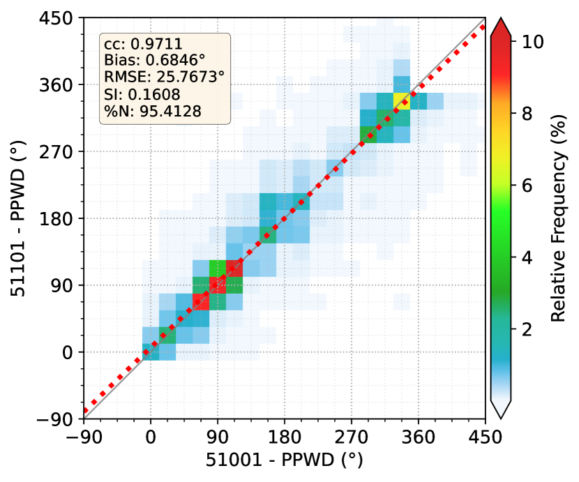
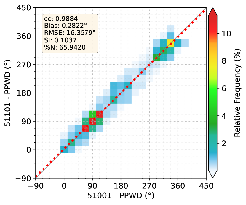
Following Hasselmann et al. (1996), is used as the critical input value for the 2PM algorithm, while the control vector is applied as input to the C4PM algorithm. This control vector imposes the following limits on parameter discrepancies within a matchup: the smallest significant wave height must be at least of the largest significant wave height in the same matchup; similar limitations apply to discrepancies in peak wave periods and peak directional spreads. Additionally, cross-assigned peak wave directions cannot differ by more than . Figure 10 illustrates the results of this comparison. Both methods exhibit negligible bias, high correlation coefficients, and low for all partitioned integrated wave parameters. However, closer examination of Figure 10[aceg], which displays the 2PM results, reveals the presence of outliers, indicating the occurrence of unlikely matchups. Such outliers, while rare, may pose challenges in applications such as data assimilation. Notably, these outliers persist even when the critical value for 2PM is significantly reduced (plots not shown). In contrast, Figure 10[bdfh], presenting the C4PM results, shows matchups tightly clustered around the 1:1 line, indicating the absence of outliers. This result highlights the effectiveness of C4PM in controlled matchup formation, further demonstrating its superiority in avoiding spurious matches.

5 Summary and Conclusions
Cross-assignment of wave spectra represents a combinatorial optimization challenge in physical oceanography. The core question is how to determine the best matching between partitions of wave spectra from different sources, specifically those whose oceanic characteristics exhibit the highest level of concordance. Addressing this problem requires a reliable method for measuring the similarity between partitions and a robust criterion to determine when pairs of partitions should form the cross-assignment.
This work proposes a novel cross-assignment methodology based on a spectral distance that incorporates four integrated wave parameters, termed the Controlled Four-Parameter Method (C4PM), which offers a high degree of customizability, enabling the assignment of distinct weights to the integrated wave parameters during the distance calculation while also allowing for a priori control of discrepancies among the corresponding parameters throughout the cross-assignment process.
To evaluate the proposed method, we compared C4PM with an existing approach based on a two-parameter spectral distance (denoted as 2PM). Thousands of data points from two buoys located 13 km apart were analyzed. The experiments explored the progression of cutoff values for each technique and their qualitative impact on the resulting groups of matchups. The results consistently demonstrated the superiority of C4PM over 2PM in nearly all aspects.
The weighted semimetric underlying C4PM proved to be well-scaled, providing superior capability in identifying matches with highly concordant oceanic features. In contrast, the spectral distance employed in 2PM exhibited limitations, allowing for the formation of mismatched pairs in numerous cases. When operating with very strict cutoff values, C4PM identified only perfect matches, i.e., measurements from nearly identical pairs of partitions, while 2PM produced a significant proportion of relatively poor matches even within the same cutoff range.
Further analysis, which divided the total set of possible matches into quintiles based on cutoff values, revealed that C4PM consistently outperformed 2PM across all groups, particularly in the first three quintiles. The values achieved by C4PM for each partitioned integrated wave parameter were consistently lower than those of 2PM, highlighting the accuracy of its matchups. This distinction was further underscored by the presence of outliers in the 2PM results, which persisted even when stricter cutoff values were applied. These outliers, indicative of poorer match quality, were absent in the C4PM results, demonstrating the robustness of its controlled matchup formation.
C4PM’s ability to assign specific weights and variability limits to each parameter provides a level of flexibility that enables tailored cross-assignments to suit the requirements of different datasets and applications. Furthermore, its negligible computational overhead and planned release as an open-source Python package enhance its accessibility and practicality for broader use. In summary, the results presented here demonstrate significant improvements over traditional spectral distance methods for the cross-assignment of directional wave spectra. C4PM is a highly effective tool for wave data assimilation, where precise cross-assignments are critical for improving the reliability and accuracy of forecast models.
Appendix A Appendix - Statistics and wave parameters
Tables 7 and 8 provide the formulas for the statistical parameters and wave parameters, respectively.
| Parameter | Expression |
|---|---|
| mean | , |
| \addstackgap[.5] bias | |
| \addstackgap[.5] root mean square error () | |
| \addstackgap[.5] Scatter index (SI) | |
| \addstackgap[.5] Pearson correlation coefficient () |
| Parameter | Expression |
|---|---|
| \addstackgap[.5] | |
| \addstackgap[.5] | |
| \addstackgap[.5] |
References
- (1)
- Aouf et al. (2021) Aouf, L., Hauser, D., Chapron, B., Toffoli, A., Tourain, C. & Peureux, C. (2021), ‘New directional wave satellite observations: Towards improved wave forecasts and climate description in southern ocean’, Geophysical Research Letters 48(5), e2020GL091187. e2020GL091187 2020GL091187.
- Aouf et al. (2006) Aouf, L., Lefevre, J.-M. & Hauser, D. (2006), ‘Assimilation of directional wave spectra in the wave model wam: An impact study from synthetic observations in preparation for the swimsat satellite mission’, Journal of Atmospheric and Oceanic Technology 23(3), 448 – 463.
- Ardhuin et al. (2019) Ardhuin, F., Stopa, J. E., Chapron, B., Collard, F., Husson, R., Jensen, R. E., Johannessen, J., Mouche, A., Passaro, M., Quartly, G. D., Swail, V. & Young, I. (2019), ‘Observing sea states’, Frontiers in Marine Science 6.
- Cavaleri et al. (2007) Cavaleri, L., Alves, J.-H., Ardhuin, F., Babanin, A., Banner, M., Belibassakis, K., Benoit, M., Donelan, M., Groeneweg, J., Herbers, T., Hwang, P., Janssen, P., Janssen, T., Lavrenov, I., Magne, R., Monbaliu, J., Onorato, M., Polnikov, V., Resio, D., Rogers, W., Sheremet, A., McKee Smith, J., Tolman, H., van Vledder, G., Wolf, J. & Young, I. (2007), ‘Wave modelling – the state of the art’, Progress in Oceanography 75(4), 603–674.
- Earle et al. (1999) Earle, M. D., Steele, K. & Wang, D. W. (1999), ‘Use of advanced directional wave spectra analysis methods’, Ocean Engineering 26, 1421–1434.
- Gerling (1992) Gerling, T. W. (1992), ‘Partitioning sequences and arrays of directional ocean wave spectra into component wave systems’, Journal of Atmospheric and Oceanic Technology 9(4), 444 – 458.
- Hanson & Phillips (2001) Hanson, J. L. & Phillips, O. M. (2001), ‘Automated analysis of ocean surface directional wave spectra’, Journal of Atmospheric and Oceanic Technology 18(2).
- Hasselmann et al. (1996) Hasselmann, S., Brüning, C., Hasselmann, K. & Heimbach, P. (1996), ‘An improved algorithm for the retrieval of ocean wave spectra from Synthetic Aperture Radar image spectra’, Journal of Geophysical Research: Oceans 101(C7), 16615–16629.
- Hauser et al. (2021) Hauser, D., Tourain, C., Hermozo, L., Alraddawi, D., Aouf, L., Chapron, B., Dalphinet, A., Delaye, L., Dalila, M., Dormy, E., Gouillon, F., Gressani, V., Grouazel, A., Guitton, G., Husson, R., Mironov, A., Mouche, A., Ollivier, A., Oruba, L., Piras, F., Rodriguez Suquet, R., Schippers, P., Tison, C. & Tran, N. (2021), ‘New observations from the swim radar on-board cfosat: Instrument validation and ocean wave measurement assessment’, IEEE Transactions on Geoscience and Remote Sensing 59(1), 5–26.
- Jiang et al. (2022) Jiang, H., Mironov, A., Ren, L., Babanin, A. V., Wang, J. & Mu, L. (2022), ‘Validation of wave spectral partitions from swim instrument on-board cfosat against in situ data’, IEEE Transactions on Geoscience and Remote Sensing 60, 1–13.
- Kuik et al. (1988) Kuik, A. J., van Vledder, G. P. & Holthuijsen, L. H. (1988), ‘A method for the routine analysis of pitch-and-roll buoy wave data’, Journal of Physical Oceanography 18(7), 1020 – 1034.
- Li & Saulter (2012) Li, J.-G. & Saulter, A. (2012), ‘Assessment of the updated envisat asar ocean surface wave spectra with buoy and altimeter data’, Remote Sensing of Environment 126, 72–83.
- Portilla-Yandún et al. (2015) Portilla-Yandún, J., Cavaleri, L. & Van Vledder, G. P. (2015), ‘Wave spectra partitioning and long term statistical distribution’, Ocean Modelling 96, 148–160. Waves and coastal, regional and global processes.
- Portilla-Yandún et al. (2019) Portilla-Yandún, J., Valladares, C. & Violante-Carvalho, N. (2019), ‘A hybrid physical-statistical algorithm for sar wave spectra quality assessment’, IEEE Journal of Selected Topics in Applied Earth Observations and Remote Sensing 12(10), 3943–3948.
- Ricondo et al. (2023) Ricondo, A., Cagigal, L., Rueda, A., Hoeke, R., Storlazzi, C. D. & Méndez, F. J. (2023), ‘Hywaves: Hybrid downscaling of multimodal wave spectra to nearshore areas’, Ocean Modelling 184, 102210.
- Santos et al. (2021) Santos, F. M., Santos, A. L., Violante-Carvalho, N., Carvalho, L. M., Brasil-Correa, Y. O., Portilla-Yandun, J. & Romeiser, R. (2021), ‘A simulator of synthetic aperture radar (sar) image spectra: the applications on oceanswell waves’, International Journal of Remote Sensing 42(8), 2981–3001.
- Smit et al. (2021) Smit, P., Houghton, I., Jordanova, K., Portwood, T., Shapiro, E., Clark, D., Sosa, M. & Janssen, T. (2021), ‘Assimilation of significant wave height from distributed ocean wave sensors’, Ocean Modelling 159, 101738.
- Violante-Carvalho et al. (2005) Violante-Carvalho, N., Robinson, I. S. & Schulz-Stellenfleth, J. (2005), ‘Assessment of ers synthetic aperture radar wave spectra retrieved from the max-planck-institut (mpi) scheme through intercomparisons of 1 year of directional buoy measurements’, Journal of Geophysical Research: Oceans 110(C7).
- Wang et al. (2020) Wang, X., Husson, R., Jiang, H., Chen, G. & Gao, G. (2020), ‘Evaluation on the capability of revealing ocean swells from sentinel-1a wave spectra measurements’, Journal of Atmospheric and Oceanic Technology 37(7), 1289 – 1304.
- Wu et al. (2024) Wu, L., Sahlée, E., Nilsson, E. & Rutgersson, A. (2024), ‘A review of surface swell waves and their role in air–sea interactions’, Ocean Modelling 190, 102397.